Fair Spatial Indexing: A paradigm for Group Spatial Fairness

Abstract.

Machine learning (ML) is playing an increasing role in decision-making tasks that directly affect individuals, e.g., loan approvals, or job applicant screening. Significant concerns arise that, without special provisions, individuals from under-privileged backgrounds may not get equitable access to services and opportunities. Existing research studies fairness with respect to protected attributes such as gender, race or income, but the impact of location data on fairness has been largely overlooked. With the widespread adoption of mobile apps, geospatial attributes are increasingly used in ML, and their potential to introduce unfair bias is significant, given their high correlation with protected attributes. We propose techniques to mitigate location bias in machine learning. Specifically, we consider the issue of miscalibration when dealing with geospatial attributes. We focus on spatial group fairness and we propose a spatial indexing algorithm that accounts for fairness. Our KD-tree inspired approach significantly improves fairness while maintaining high learning accuracy, as shown by extensive experimental results on real data.

1. Introduction

Recent advances in machine learning (ML) led to its adoption in numerous decision-making tasks that directly affect individuals, such as loan evaluation or job application screening. Several studies (Pessach and Shmueli, 2022; Berk et al., 2021; Mhasawade et al., 2021) pointed out that ML techniques may introduce bias with respect to protected attributes such as race, gender, age or income. The last years witnessed the introduction of fairness models and techniques that aim to ensure all individuals are treated equitably, focusing especially on conventional protected attributes (like race or gender). However, the impact of geospatial attributes on fairness has not been extensively studied, even though location information is being increasingly used in decision-making for novel tasks, such as recommendations, advertising or ride-sharing. Conventional applications may also often rely on location data, e.g. allocation of local government resources, or crime prediction by law enforcement using geographical features. For example, the Chicago Police Department releases monthly crime datasets (chi, 2015) and classifies neighborhoods based on their crime risk level. Subsequently, the risk level is used to determine vehicle and house insurance premiums, which are increased to reflect the risk level, and in turn, result in additional financial hardship for individuals from under-privileged groups.

Fairness for geospatial data is a challenging problem, due to two main factors: (i) data are more complex than conventional protected attributes such as gender or race, which are categorical and have only a few possible values; and (ii) the correlation between locations and protected attributes may be difficult to capture accurately, thus leading to hard-to-detect biases.

We consider the case of group fairness (Dwork and Ilvento, 2018), which ensures no significant difference in outcomes occurs across distinct population groups (e.g., females vs. males). In our setting, groups are defined with respect to geospatial regions. The data domain is partitioned into disjoint regions, and each of them represents a group. All individuals whose locations belong to a certain region are assigned to the corresponding group. In practice, a spatial group can correspond to a zip code, a neighborhood, or a set of city blocks. Our objective is to support arbitrary geospatial partitioning algorithms, which can handle the needs of applications that require different levels of granularity in terms of location reporting. Spatial indexing (Wang et al., 2020; Eldawy and Mokbel, 2015; Zhang et al., 2016) is a common approach used for partitioning, and numerous techniques have been proposed that partition the data domain according to varying criteria, such as area, perimeter, data point count, etc. We build upon existing spatial indexing techniques, and adapt the partition criteria to account for the specific goals of fairness. By carefully combining geospatial and fairness criteria in the partitioning strategies, one can obtain spatial fairness while still preserving the useful spatial properties of indexing structures (e.g., fine-level clustering of the data).

Specifically, we consider a set of partitioning criteria that combines physical proximity and calibration error. Calibration is an essential concept in classification tasks which quantifies the quality of a classifier. Consider a binary classification task, such as a loan approval process. Calibration measures the difference between the observed and predicted probabilities of any given point being labeled in the positive class. If one partitions the data according to some protected attribute, then the expectation would be that the probability should be the same across both groups (e.g., males and females should have an equal chance, on aggregate, to be approved for a loan). If the expected and actual probabilities are different, that represents a good indication of unfair treatment.

Our proposed approach builds a hierarchical spatial index structure by using a composite split metric, consisting of both geospatial criteria (e.g., compact area) and miscalibration error. In doing so, it allows ML applications to benefit from granular geospatial information, while at the same time ensuring that no significant bias is present in the learning process.

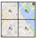
(a) Neighborhoods Partitioning

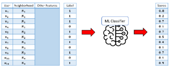
(b) Generation of Classifier Scores

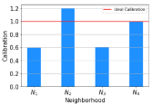
(c) Calibration of Neighborhoods

Figure 1. An example of the miscalibration problem with respect to neighborhoods.

Our specific contributions include:

• We identify and formulate the problem of spatial group fairness, an important concept which ensures that geospatial information can be used reliably in a classification task, without introducing, intentionally or not, biases against individuals from underprivileged groups;

• We propose a new metric to quantify unfairness with respect to geospatial boundaries, called Expected Neighborhood Calibration Error (ENCE);

• We propose a technique for fair spatial indexing that builds on KD-trees and considers both geospatial and fairness criteria, by lowering miscalibration and minimizing ENCE;

• We perform an extensive experimental evaluation on real datasets, showing that the proposed approach is effective in enforcing spatial group fairness while maintaining data utility for classification tasks.

The rest of the paper is organized as follows: Section 2 provides background and fundamental definitions. Section 3 reviews related work. We introduce the proposed fair index construction technique in Section 4. Section 5 presents the results of our empirical evaluation, followed by conclusions in Section 6.

2. Background

2.1. System Architecture

We consider a binary classification task $T$ over a dataset $D$ of individuals $u_{1},\,...,\,u_{|D|}$. The feature set recorded for $u_{i}$ is denoted by $\boldsymbol{x_{i}}\in\mathbb{R}^{l}$, and its corresponding label by $y_{i}\in\{0,1\}$. Each record consists of $l$ features, including an attribute called neighborhood, which captures an individual’s location, and is the main focus of our approach. The sets of all input data and labels are denoted by $\mathcal{X}$ and $\mathcal{Y}$, respectively. A classifier $h(.)$ is trained over the input data resulting in $h(\mathcal{X})=(\hat{Y},\hat{S})$ where $\mathcal{\hat{Y}}=\{\hat{y}_{1},...,\hat{y}_{|D|}\}$ is the set of predicted labels ($\hat{y}_{i}\in\{0,1\}$) and $\mathcal{S}=\{s_{1},...,s_{|D|}\}$ is the set of confidence scores ($s_{i}\in[0,1]$) for each label.

The dataset’s neighborhood feature indicates the individual’s spatial group. We assume the spatial data domain is split into a set of partitions of arbitrary granularity. Without loss of generality, we consider a $U\times V$ grid overlaid on the map. The grid is selected such that its resolution captures adequate spatial accuracy as required by application needs. A set of neighborhoods is a non-overlapping partitioning of the map that covers the entire space, with the $i^{th}$ neighborhood denoted by $N_{i}$, and the set of neighborhoods denoted by $\mathcal{N}$.

Figure 1 illustrates the system overview. Figure 1a shows the map divided into $4$ non-overlapping partitions $\mathcal{N}=\{N_{1},N_{2},N_{3},N_{4}\}$. The neighborhood is recorded for each individual $u_{1},...,u_{11}$ together with other features, and a classifier is trained over the data. The classifier’s output is the confidence score for each entry which turns into a class label by setting a threshold.

2.2. Fairness Metric

Our primary focus is to achieve spatial group fairness using as metric the concept of calibration (Naeini et al., 2015; Pleiss et al., 2017), described in the following.

In classification tasks, it is desirable to have scores indicating the probability that a test data record belongs to a certain class. Probability scores are especially important in ranking problems, where top candidates are selected based on relative quantitative performance. Unfortunately, it is not granted that confidence scores generated by a classifier can be interpreted as probabilities. Consider a binary classifier that indicates an individual’s chance of committing a crime after their release from jail (recidivism). If two individuals $u_{1}$ and $u_{2}$ get confidence scores $0.4$ and $0.8$, this cannot be directly interpreted as the likelihood of committing a crime by $u_{2}$ being twice as high as for $u_{1}$. The model calibration aims to alleviate precisely this shortcoming.

Definition 1.

(Calibration). An ML model is said to be calibrated if it produces calibrated confidence scores. Formally, outcome score $R$ is calibrated if for all scores $r$ in support of $R$ it holds that

(1) $$P(y=1|R=r)=r$$

This condition means that the set of all instances assigned a score value $r$ contains an $r$ fraction of positive instances. The metric is a group-level metric. Suppose there exist $10$ people who have been assigned a confidence score of $0.7$. In a well-calibrated model, we expect to have $7$ individuals with positive labels among them. Thus, the probability of the whole group is $0.7$ to be positive, but it does not indicate that every individual in the group has this exact chance of receiving a positive label.

To measure the amount of miscalibration for the whole model or for an output interval, the ratio of two key factors need to be calculated: expected confidence scores and the expected value of true labels. Abiding by the convention in (Naeini et al., 2015), we use functions $o(.)$ and $e(.)$ to return the true fraction of positive instances and the expected value of confidence scores, respectively. For example, the calibration of the model in Figure 1b is computed as:

(2) $$\dfrac{e(h)}{o(h)}=\dfrac{(\sum_{u\in D}\hat{p}_{u})/|D|}{(\sum_{u\in D}y_{u})/|D|}=\dfrac{5.2/11}{7/11}\approx.742$$

Perfect calibration is achieved when a specific ratio is equal to one. Ratios that are above or below one are considered miscalibration cases. Another way to measure the calibration error is by using the absolute value of the difference between two values, denoted by $|e(h)-o(h)|$, with the ideal value being zero. In this work, the second method is utilized, as it eliminates the division by zero problem that may arise from neighborhoods with low populations.

2.3. Problem Formulation

Even when a model is overall well-calibrated, it can still lead to unfair treatment of individuals from different neighborhoods. In order to achieve spatial group fairness, we must have a well-calibrated model with respect to all neighborhoods. The existence of calibration error in a neighborhood can result in classifier bias and lead to systematic unfairness against individuals from that neighborhood (in Section 5, we support this claim with real data measurements).

Definition 2.

(Calibration for Neighborhoods). Given neighborhood set $\mathcal{N}=\{N_{1},...,N_{t}\}$, we say that the score $R$ is calibrated in neighborhood $N_{i}$ if for all the scores $r$ in support of $R$ it holds that

(3) $$P(y=1|R=r,N=N_{i})=r,\;\;\;\;\;\;\forall i\in[1,t]$$

The following equations can be used to measure the amount of miscalibration with respect to neighborhood $N_{i}$,

(4) $$\dfrac{e(h|N=N_{i})}{o(h|N=N_{i})}\;\;\;\text{ or }\;\;\;|e(h|N=N_{i})-o(h|N=N_{i})|$$

Going back to the example in Figure 1d, the calibration amount for neighborhoods $N_{1}$ to $N_{4}$ is visualized on a plot. Neighborhood $N_{4}$ is well-calibrated, whereas the others suffer from miscalibration.

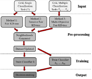
Figure 2. Overview of the proposed mitigation techniques.

Problem 1.

Given m binary classification tasks $T_{1},T_{2},...,T_{m}$, we seek to partition the space into continuous non-overlapping neighborhoods such that for each decision-making task, the trained model is well-calibrated for all neighborhoods.

2.4. Evaluation Metrics

A commonly used metric to evaluate the calibration of a model is Expected Calibration Error (ECE) (Guo et al., 2017). The goal of ECE (detailed in Appendix A.1) is to understand the validity of output confidence scores. However, our focus is on identifying the calibration error imposed on different neighborhoods. Therefore, we extend ECE and propose the Expected Neighborhood Calibration Error (ENCE) that captures the calibration performance over all neighborhoods.

Definition 3.

(Expected Neighborhood Calibration Error). Given $t$ non-overlapping geospatial regions $\mathcal{N}=\{N_{1},...,N_{t}\}$ and a classifier $h$ trained over data located in these neighborhoods, the ENCE metric is calculated as:

(5) $$\text{ENCE}=\sum_{i=1}^{t}\dfrac{|N_{i}|}{|D|}|\text{o}(N_{i})-e(N_{i})|$$

where $o(N_{i})$ and $e(N_{i})$ return the true fraction of positive instances and the expected value of confidence scores for instances in $N_{i}$.

Table 1. Summary of Notations.

Symbol	Description
$k$	Number of features
$D=\{u_{1},...,u_{|D|}\}$	Dataset of individuals
$(x_{i},y_{i})$	(Set of features, true label) for $u_{i}$
$D=[\mathcal{X},\mathcal{Y}]$	Dataset with user features and labels
$\mathcal{\hat{Y}}\texttt{=}\{\hat{y}_{1},..,\hat{y}_{|D|}\}$	Set of predicted labels
$\mathcal{S}=\{s_{1},...,s_{|D|}\}$	Set of confidence scores
$\mathcal{N}=\{N_{1},...,N_{t}\}$	Set of neighborhoods
$U\times V$	Base grid resolution
$T$	Binary classification task
$m$	Number of binary classification tasks
$t$	Number of neighborhoods
$t_{h}$	Tree height

3. Related Work

Fairness Notions. There exist two broad categories of fairness notions (Mehrabi et al., 2021; Caton and Haas, 2020): individual fairness and group fairness. In group fairness, individuals are divided into groups according to a protected attribute, and a decision is said to be fair if it leads to a desired statistical measure across groups. Some prominent group fairness metrics are calibration (Pleiss et al., 2017), statistical parity (Kusner et al., 2017)(Dwork et al., 2012), equalized odds (Hardt et al., 2016), treatment equality (Berk et al., 2021), and test fairness (Chouldechova, 2017). Individual fairness notions focus on treating similar individuals the same way. Similarity may be defined with respect to a particular task (Dwork et al., 2012; Joseph et al., 2016).

Spatial Fairness. Neighborhoods or individual locations are commonly used features for decision-making in government agencies, banks, etc. Unfairness may arise in tasks such as mortgage lending (Lee and Floridi, 2021), job recruitment (Faliagka et al., 2012), admission to schools (Benabbou et al., 2019), and crime risk prediction (Wang et al., 2022). In (Wang et al., 2022), recidivism prediction models constructed using data from one location tend to perform poorly when they are used to predict recidivism in another location. The authors in (Riederer and Chaintreau, 2017) formulate a loss function for individual fairness in social media and location-based advertisements. Pujol et al. (Pujol and Machanavajjhala, 2021) demonstrate the unequal impact of differential privacy on neighborhoods. Several attempts have been made to apply fairness notions for clustering datapoints in the Cartesian space. The notion in (Kleindessner et al., 2020) defines clustering conducted for a point as fair if the average distance to the points in its own cluster is not greater than the average distance to the points in any other cluster. The authors in (Mahabadi and Vakilian, 2020) focus on defining individual fairness for $k$-median and $k$-means algorithms. Clustering is defined to be individually fair if every point expects to have a cluster center within a particular radius.

Unfairness Mitigation techniques can be categorized into three broad groups: pre-processing, in-processing, and post-processing. Pre-processing algorithms achieve fairness by focusing on the classifier’s input data. Some well-known techniques include suppression of sensitive attributes, change of labels, reweighting, representation learning, and sampling (Kamiran and Calders, 2012). In-processing techniques achieve fairness during training by adding new terms to the loss function (Kamishima et al., 2012) or including more constraints in the optimization. Post-processing techniques sacrifice the utility of output confidence scores and align them with the fairness objective (Platt et al., 1999).

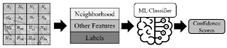
(a) Initial execution of classifier.

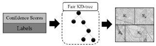
(b) Re-districting the map based on fairness objective.

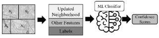
(c) Training classifier based on re-districted neighborhoods.

Figure 3. Overview of Fair KD-tree algorithm.

4. Spatial Fairness through Indexing

We introduce several algorithms that achieve group spatial fairness by constructing spatial index structures in a way that takes into account fairness considerations when performing data domain splits. We choose KD-trees as a starting point for our solutions, due to their ability to adapt to data density, and their property of covering the entire data domain (as opposed to structures like R-trees that may leave gaps within the domain).

Figure 2 provides an overview of the proposed solution. Our input consists of a base grid with an arbitrarily-fine granularity overlaid on the map, the attributes/features of individuals in the data, and their classification labels. The attribute set includes individual location, represented as the grid cell enclosing the individual. We propose a suite of three alternative algorithms for fairness, which are applied in the pre-processing phase of the ML pipeline and lead to the generation of new neighborhood boundaries. Once spatial partitioning is completed, the location attribute of each individual is updated, and classification is performed again.

The proposed algorithms are:

• Fair KD-tree is our primary algorithm and it re-districts spatial neighborhoods based on an initial classification of data over a base grid. Fair KD-tree can be applied to a single classification task.

• Iterative Fair KD-tree improves upon Fair KD-tree by refining the initial ML scores at every height of the index structure. It incurs higher computational complexity but provides improved fairness.

• Multi-Objective Fair KD-tree enables Fair KD-trees for multiple classification tasks. It leads to the generation of neighborhoods that fairly represent spatial groups for multiple objectives.

Next, we prove an important result that applies to all proposed algorithms, which states that any non-overlapping partitioning of the location domain has a weighted average calibration greater or equal to the overall model calibration. The proofs of all theorems are provided in Appendix A.

Theorem 1.

For a given model $h$ and a complete non-overlapping partitioning of the space $\mathcal{N}=\{N_{1},N_{2},...,N_{t}\}$, ENCE is lower-bounded by the overall calibration of the model.

A broader statement can also be proven, showing that further partitioning leads to poorer ENCE performance.

Theorem 2.

Consider a binary classifier $h$ and two complete non-overlapping partitioning of the space $\mathcal{N}_{1}$ and $\mathcal{N}_{2}$. If $\mathcal{N}_{2}$ is a sub-partitioning of $\mathcal{N}_{1}$, then:

(6) $$\text{ENCE}(N_{1})\leq\text{ENCE}(N_{2})$$

Neighborhood set $\mathcal{N}_{2}$ is a sub-partitioning of $\mathcal{N}_{1}$ if for every $N_{i}\in\mathcal{N}_{1}$, there exists a set of neighborhoods in $\mathcal{N}_{2}$ such that their union is $N_{i}$.

Algorithm 1 Fair KD-tree

1: Input: Grid ($U\times V$), Features ($\mathcal{X}$), Labels ($\mathcal{Y}$), Height ($t_{h}$).

2: Output: New neighborhoods and updated feature set

3:function FairKDtree($N,\mathcal{X},\mathcal{Y},\mathcal{S},t_{h}$)

4:     if $t_{h}=0$ then

5:         $\mathcal{N}\leftarrow\mathcal{N}+N$

6:         return $True$      

7:     $axis\leftarrow\,t_{h}$ mod 2

8:     $L_{k^{*}},\,R_{k^{*}}\leftarrow$ SplitNeighborhood$(N,\mathcal{Y},\mathcal{S},axis)$

9:     Run FairKDtree($L_{k^{*}},\mathcal{X},\mathcal{Y},\mathcal{S},t_{h}-1$)

10:     Run FairKDtree($R_{k^{*}},\mathcal{X},\mathcal{Y},\mathcal{S},t_{h}-1$)

11:$N_{1}\leftarrow$ Grid

12:Global $\mathcal{N}\leftarrow\{\}$

13:Set all neighborhoods in $\mathcal{X}$ to $N_{1}$

14:Scores ($\mathcal{S}$) $\leftarrow$ Train ML model on $\mathcal{X}$ and $\mathcal{Y}$

15:Neighborhoods ($\mathcal{N})\leftarrow$ Run $FairKDtree(N_{1},\mathcal{X},\mathcal{Y},\mathcal{S},t_{h})$

16:Update neighborhoods in $\mathcal{X}$

17:return $\mathcal{N},\,\mathcal{X}$

Algorithm 2 Split Neighborhood

1: Input: Neighborhood ($N$), Confidence Scores ($\mathcal{S}$), Labels ($\mathcal{Y}$), Axis.

2: Output: Non-overlapping split of $N$ into two neighborhoods

3:function SplitNeighborhood($N,\mathcal{S},\mathcal{Y},axis$)

4:     if $axis=1$ then

5:         $N\leftarrow$ Transpose of $N$      

6:     $U^{\prime}\times V^{\prime}\leftarrow$ Dimensions of $N$

7:     for $k=1...U^{\prime}$ do

8:         $L_{k}\leftarrow$ Neighborhoods in $1...k$

9:         $R_{k}\leftarrow$ Neighborhoods in $k+1...U$

10:         $z_{i}\leftarrow$ Compute Equation (9) for $L_{k}$ and $R_{k}$      

11:     $k^{*}\leftarrow$ $\arg\min_{k}\;\;z_{k}$

12:     return $L_{k^{*}}$, $R_{k^{*}}$

4.1. Fair KD-tree

We build a KD-tree index that partitions the space into non-overlapping regions according to a split metric that takes into account the miscalibration metric within the regions resulting after each split. Figure 3 illustrates this approach, which consists of three steps. Algorithm 1 presents the pseudocode of the approach.

Step 1. The base grid is used as input, where the location of each individual is represented by the identifier of their enclosing grid cell. This location attribute, alongside other features, is used as input to an ML classifier $h$ for training. The classifier’s output is a set of confidence scores $\mathcal{S}$, as illustrated in Figure 3a. Once confidence scores are generated, the true fraction of positive instances and the expected value of predicted confidence scores of the model with respect to neighborhoods can be calculated as follows:

(7) $$e(h|N=N_{i})=\dfrac{1}{|N_{i}|}(\sum_{u\in N_{i}}s_{u})\;\;\;\;\;\;\forall i\in[1,t]$$

(8) $$o(h|N=N_{i})=\dfrac{1}{|N_{i}|}(\sum_{u\in N_{i}}y_{u})\;\;\;\;\;\;\forall i\in[1,t]$$

where $t$ is the number of neighborhoods.

Algorithm 3 Iterative Fair KD-tree

1: Input: Grid ($U\times V$), Features ($\mathcal{X}$), Labels ($\mathcal{Y}$), Height ($t_{h}$).

2: Output: New neighborhoods and updated feature set

3:$N_{1}\leftarrow$ Grid

4:Set all neighborhoods in $\mathcal{X}$ to $N_{1}$

5:$\mathcal{N}\leftarrow\{N_{1}\}$

6:while $t_{h}>0$ do

7:     Scores ($\mathcal{S}$) $\leftarrow$ Train ML model on $\mathcal{X}$ and $\mathcal{Y}$

8:     $\mathcal{N_{\text{new}}}\leftarrow\{\}$

9:     for $N_{i}\;\text{in}\;\mathcal{N}$ do

10:         $L,R\leftarrow$ SplitNeighborhood$(N_{i},\mathcal{S},\mathcal{Y},t_{h}\%2)$

11:         $\mathcal{N_{\text{new}}}\leftarrow\mathcal{N_{\text{new}}}+{L,R}$

12:              $\mathcal{N}\leftarrow\mathcal{N_{\text{new}}}$

13:     Update neighborhoods in $\mathcal{X}$ based on $\mathcal{N}$

14:     $t_{h}\leftarrow t_{h}-1$

15:return $\mathcal{N},\,\mathcal{X}$

Step 2. This step performs the actual partitioning, by customizing the KD-tree split algorithm with a novel objective function. KD-trees are binary trees where a region is split into two parts, typically according to the median value of the coordinate across one of the dimensions (latitude or longitude). Instead, we select the division index that minimizes fairness metric, i.e., ENCE miscalibration. Confidence scores and labels resulted from the previous training step are used as input for the split point decision. For a given tree node, assume the corresponding partition covers $U^{\prime}\times V^{\prime}$ cells of the entire $U\times V$ grid. Without loss of generality, we consider partitioning on the horizontal axis (i.e., row-wise). The aim is to find an index $k$ which groups rows $1$ to $k$ into one node and rows $k+1$ to $U^{\prime}$ into another, such that the fairness objective is minimized. Let $L_{k}$ and $R_{k}$ denote the left and right regions generated by splitting on index $k$. The fairness objective for index $k$ is:

(9) $$z_{k}=\big{|}\;|L_{k}|\times|o(L_{k})-e(L_{k})|-|R_{k}|\times|o(R_{k})-e(R_{k})\;|\big{|}$$

In the above equation, $|L_{k}|$ and $|R_{k}|$ return the number of data entries in the left and right regions, respectively. The intuition behind the objective function is to minimize the model miscalibration difference as we heuristically move forward. Two key points about the above function are: (i) the formulation of calibration is used in linear format due to the possibility of a zero denominator, and (ii) the calibration values are weighted by their corresponding regions’ cardinalities. The optimal index $k^{*}$ is selected as:

(10) $$k^{*}=\arg\min_{k}\;\;z_{k}\;\;\;$$

Step 3. On completion of the fair KD-tree algorithm, the index leaf set provides a non-overlapping partitioning of the map. In the algorithm’s final step, the neighborhood of each individual in the dataset is updated according to the leaf set and used for training.

The Fair KD-tree pseudocode is provided in Algorithms 1 and 2. The latter returns the split point based on the fairness objective, and it is being called several times in Algorithm 1. This function will also be used within the Iterative KD-tree algorithm.

Theorem 3.

For a given dataset $D$, the required number of neighborhoods $t$ and the model $h$, the computational complexity of Fair KD-tree is $\mathcal{O}(|D|\times\lceil\log(t)\rceil)+\mathcal{O}(h)$.

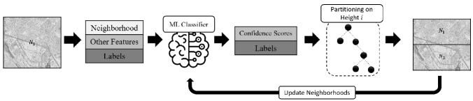
Figure 4. Overview of Iterative Fair KD-tree algorithm.

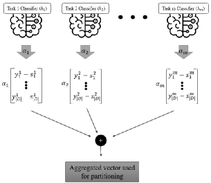
Figure 5. Aggregation in Multi-Objective Fair KD-tree.

4.2. Iterative Fair KD-tree

One drawback of the Fair KD-tree algorithm is its sensitivity to the initial execution of the model, which uses the baseline grid to generate confidence scores. Even though the space is recursively partitioned following the initial steps, the scores are not re-computed until the index construction is finalized. The iterative fair KD-tree addresses this limitation by re-training the model and computing updated confidence scores after each split (i.e., at each level of the tree). A refined version of ML scores is used at every height of the tree, leading to a more fair redistricting of the map.

Similar to the Fair KD-tree algorithm, the baseline grid is initially used, and all grid cells are considered to be in the same neighborhood (i.e., a single spatial group covering the entire domain). The algorithm is implemented in $t_{h}$ iterations with the root node corresponding to the initial point (entire domain). As opposed to the Fair KD-tree algorithm that follows Depth First Search (DFS) recursion, the Iterative Fair KD-tree algorithm is based on Breadth First Search (BFS) traversal. Therefore, all nodes in the given height $i-1$ are completed before moving forward to the height $i$. Suppose we are in the $i^{th}$ level of the tree, and all nodes at that level are generated. Note that, the set of nodes at the same height represents a non-overlapping partitioning of the grid. The algorithm continues by updating the neighborhoods at height $i$ based on the $i-1$ level partitioning. Then, the updated dataset is used to train a new model, thus updating confidence scores for each individual.

Algorithm 3 presents the Iterative Fair KD-tree algorithm. Let $\mathcal{N}$ denote the set of all neighborhoods at level $i$ of the tree. For each neighborhood $N_{i}\in\mathcal{N}$, Iterative Fair KD-tree splits the region $N_{i}$ by calling the $SplitNeighborhood$ function in Algorithm 2. The split is done on the $x$-axis if $i$ is even and on the $y$-axis otherwise.

The algorithm provides a more effective way of determining a fair neighborhood partitioning by re-training the model at every tree level, but incurs higher computation complexity.

Theorem 4.

For a given dataset $D$, the required number of neighborhoods $t$ and the model $h$, the computational complexity of Iterative Fair KD-tree is $\mathcal{O}(|D|\times\lceil\log(t)\rceil)+\lceil\log(t)\rceil\times\mathcal{O}(h)$.

4.3. Multi-Objective Fair KD-tree

So far, we focused on achieving a fair representation of space given a single classification task. In practice, applications may dictate multiple classification objectives. For example, a set of neighborhoods that are fairly represented in a city budget allocation task may not necessarily result in a fair representation of a map for deriving car insurance premia. Next, we show how Fair KD-tree can be extended to incorporate multi-objective decision-making tasks.

We devise an alternative method to compute initial scores in Line 10 of Algorithm 2, which can then be called as part of Fair KD-tree in Algorithm 1. A separate classifier is trained over each task to incorporate all classification objectives. Let $h_{i}$ be the $i^{th}$ classifier trained over $D$ and label set $\mathcal{Y}_{i}$ representing the task $T_{i}$. The output of the classifier is denoted by $\mathcal{S}_{i}=\{s_{1}^{i},...,s_{|D|}^{i}\}$, where in $s_{j}^{i}$, the superscript identifies the set $\mathcal{S}_{i}$ and the subscript indicates individual $u_{j}$. Once confidence scores for all models are generated, an auxiliary vector is constructed as follows:

(11) $$\boldsymbol{v}_{i} =\begin{bmatrix}s_{1}^{i}-y_{1}^{i}\\ s_{2}^{i}-y_{2}^{i}\\ \vdots\\ s_{|D|}^{i}-y_{|D|}^{i}\end{bmatrix},\;\;\;\;\;\;\;\forall i\in[1...t]$$

To facilitate task prioritization, hyper-parameters $\alpha_{1},...,\alpha_{m}$ are introduced such that $\sum_{i\texttt{=}1}^{m}\alpha_{i}=1$ and $0\leq\alpha_{i}\leq 1$. Coefficient $\alpha_{i}$ indicates the significance of classification $T_{i}$. The complete vector used for computing the partitioning is then calculated as,

(12) $$\boldsymbol{v}_{tot}=\sum_{i\texttt{=}1}^{m}\alpha_{i}\boldsymbol{v}_{i}=\begin{bmatrix}\sum_{i\texttt{=}1}^{m}\alpha_{i}(s_{1}^{i}-y_{1}^{i})\\ \sum_{i\texttt{=}1}^{m}\alpha_{i}(s_{2}^{i}-y_{2}^{i})\\ \vdots\\ \sum_{i\texttt{=}1}^{m}\alpha_{i}(s_{|D|}^{i}-y_{|D|}^{i})\end{bmatrix}$$

In the above formulation, each row corresponds to a unique individual and captures its role in all classification tasks. Let $\boldsymbol{v}_{tot}[u_{i}]$ denote the entry corresponding to $u_{i}$ in $\boldsymbol{v}_{tot}$. Then the classification objective function in Eq. 9 is returned by:

(13) $$z_{k}=\big{|}\;|L_{k}|\times|\sum_{u_{i}\texttt{=}L_{k}}\boldsymbol{v}_{tot}[u_{i}]|\;-\;|R_{k}|\times|\sum_{u_{i}\texttt{=}R_{k}}\boldsymbol{v}_{tot}[u_{i}]\;|\big{|}$$

and the optimal split point is selected as,

(14) $$k^{*}=\arg\min_{k}\;\;z_{k}\;\;\;$$

Vector aggregation is illustrated in Figure 5.

Theorem 5.

For a given dataset $D$, the required number of neighborhoods $t$ and $m$ classification tasks modelled by $h_{1},...,h_{m}$, computational complexity of Multi-Objective Fair KD-tree is $\mathcal{O}(|D|\times\lceil\log(t)\rceil)+\sum_{i\texttt{=}1}^{m}\mathcal{O}(h_{i})$.

5. Experimental Evaluation

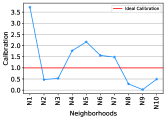
(a) EdGap (Los Angeles)

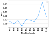
(b) EdGap (Los Angeles)

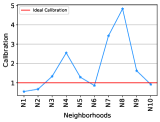
(c) EdGap (Houston)

(d) EdGap (Houston)

Figure 6. Evidence of Model Disparity on Geospatial Neighborhoods.

(a) Los Angeles (Logistic Regression)

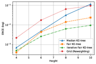
(b) Los Angeles (Decision Tree)

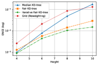
(c) Los Angeles (Naive Bayes)

(d) Houston (Logistic Regression)

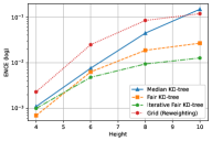
(e) Houston (Decision Tree)

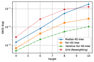
(f) Houston (Naive Bayes)

Figure 7. Performance Evaluation with respect to ENCE.

5.1. Experimental Setup

We use two real-world datasets provided by EdGap (VanWylen, [n.d.]) with $1153$ and $966$ data records respectively, containing socio-economic features (e.g., household income and family structure) of US high school students in Los Angeles, CA and Houston, Texas. Consistent with (Fischer, 2021), we use two features of average American College Testing (ACT) and the percentage of family employment as indicators to generate classification labels. The geospatial coordinates of schools are derived by linking their identification number to data provided by the National Center for Education Statistics (edu, [n.d.]).

We evaluate the performance of our proposed approaches (Fair KD-tree, Iterative Fair KD-tree, and multi-objective Fair KD-tree) in comparison with three benchmarks: (i) Median KD-tree, the standard method for KD-tree partitioning; (ii) Reweighting over grid – an adaptation of the re-weighting approach used in in (Kamiran and Calders, 2012) and deployed in geospatial tools such as IBM AI Fairness 360; and (iii) we use zip code partitioning as a baseline partitioning. All experiments are implemented in Python and executed on a $3.40$GHz core-i7 Intel processor with 16GB RAM.

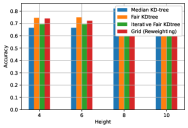
(a) Model Accuracy (Los Angeles)

(b) Training Miscalibration (Los Angeles)

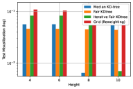
(c) Test Miscalibration (Los Angeles)

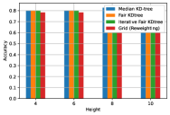
(d) Model Accuracy (Houston)

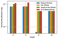
(e) Training Miscalibration (Houston)

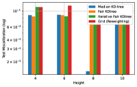
(f) Test Miscalibration (Houston)

Figure 8. Performance Evaluation with respect to other indicators.

5.2. Evidence for Disparity in Geospatial ML

First, we perform a set of experiments to measure the amount of bias that occurs when performing ML on geospatial datasets without any mitigating factors. Figure 6 captures the existing disparity with respect to widely accepted metrics of calibration error and ECE with $15$ bins. We use the ratio representation of calibration in which a closer value to $1$ represents higher calibration levels. Two logistic regression models are trained over neighborhoods in Los Angeles and Houston areas. The labels are generated by setting a threshold of $22$ on the average ACT performance of students in schools. The overall performance of models in terms of training and test calibration in Los Angeles and Texas are $(1.005,\,1.033)$ and $(0.999,\,0.958)$, respectively. Both training and test calibration are close to $1$ overall, which in a naive interpretation would indicate all schools are treated fairly. However, this is not the case when computing the same metrics on a per-neighborhood basis. Figure 6 shows miscaibration error for the top $10$ most populated zip codes. Despite the model’s acceptable outcomes overall, many individual neighborhoods suffer from severe calibration errors, leading to unfair outcomes in the most populated regions, which are often home to the under-privileged communities.

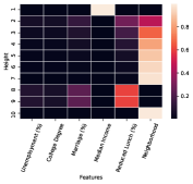
(a) Median KD-tree (Los Angeles)

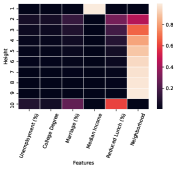
(b) Fair KD-tree (Los Angeles)

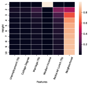
(c) Iterative Fair KD-tree (Los Angeles)

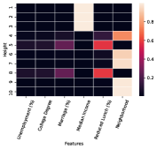
(d) Median KD-tree (Houston)

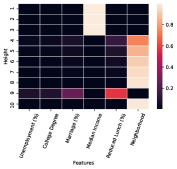
(e) Fair KD-tree (Houston)

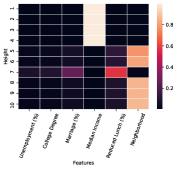
(f) Iterative Fair KD-tree (Houston)

Figure 9. Impact of features on decision-making.

5.3. Mitigation Algorithms

5.3.1. Evaluation w.r.t. ENCE Metric.

ENCE is our primary evaluation metric that captures the amount of calibration error over neighborhoods. Recall that Fair KD-tree and its extension Iterative Fair KD-tree can work for any given classification ML model. We apply algorithms for Logistic Regression, Decision Tree, and Naive Bayes classifiers to ensure diversity in models. We focus on student SAT performance following the prior work in (Fischer, 2021) by setting the threshold to $22$ for label generation. Figure 7 provides the results in Los Angeles and Houston on the EdGap dataset. The $x$-axis denotes the tree’s height used in the algorithm. Having a higher height indicates a finer-grained partitioning. The $y$-axis is log-scale.

Figure 7 demonstrates that both Fair KD-tree and Iterative Fair KD-tree outperform benchmarks by a significant margin. The improvement percentage increases as the number of neighborhoods increase, which is an advantage of our techniques, since finer spatial granularity is beneficial for most analysis tasks. The intuition behind this trend lies in the overall calibration of the model: given that the trained model is well-calibrated overall, dividing the space into a smaller number of neighborhoods is expected to achieve a calibration error closer to the overall model. This result supports Theorem 1, stating that ENCE is lower-bounded by the number of neighborhoods. Iterative Fair KD-tree behaves better, as confidence scores are updated on every tree level. The improvement achieved compared to Fair KD-trees comes at the expense of higher computational complexity. On average Fair KD-tree achieves $45\%$ better performance in terms of computational complexity. The time taken for Fair KD-tree with 10 levels is $102$ seconds, versus $189$ seconds for the iterative version.

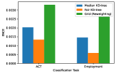
(a) Height$=4$, Los Angeles

(b) Height$=6$, Los Angeles

(c) Height$=8$, Los Angeles

(d) Height$=10$, Los Angeles

(e) Height$=4$, Houston

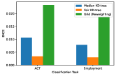
(f) Height$=6$, Houston

(g) Height$=8$, Houston

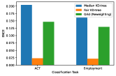
(h) Height$=10$, Houston

Figure 10. Performance evaluation of multi-objective algorithm.

5.3.2. Evaluation w.r.t. other Indicators.

In Figure 8 we evaluate fairness with respect to three other key indicators: model accuracy, training miscalibration, and test miscalibration. We focus on logistic regression, one of the most widely adopted classification units. The accuracy of all algorithms follows a similar pattern and increases at higher tree heights. This is expected, as more geospatial information can be extracted at finer granularities.

Figure 8b shows training miscalibration calculated for the overall model (a lower value of calibration error indicates better performance). Our proposed algorithms have comparable calibration errors to benchmarks, even though their fairness is far superior. To understand better underlying trends, Figure 9 provides the heatmap for the tree-based algorithms over $10$ different tree heights. The amount of contribution each feature has on decision-masking is captured using a different color code. One observation is that the model shifts focus to different features based on the height. Such sudden changes can impact the generated confidence scores and, subsequently, the overall calibration of the model. As an example, consider the median KD-tree algorithm at the height of $8$ in Los Angeles (Figure 8b): there is a sudden drop in training calibration, which can be explained by looking at the corresponding heat map in Figure 9a. At the height of $8$, the influential features on decision-making consist of different elements than the heights $4$, $6$, and $10$, leading to the fluctuation in the model calibration.

5.4. Performance of multi-objective approach.

When multi-objective criteria are used, we need a methodology to unify the geospatial boundaries generated by each task. Our proposed multi-objective fair partitioning predicated on Fair KD-trees addresses exactly this problem. In our experiments, we use the two criteria of ACT scores and employment percentage of families as the two objectives used for partitioning. These features are separated from the training dataset in the pre-processing phase and are used to generate labels. The threshold for ACT is selected as before ($22$), and the threshold for label generation based on family employment is set to $10$ percent.

Figure 10 presents the results of the Multi-Objective Fair KD-tree (to simplify chart notation, we use the ‘Fair KD-tree’ label). We choose a $\alpha$ value of $0.5$ to give equal weight to both objectives. We emphasize that, the output of the Multi-Objective Fair KD-tree is a single non-overlapping partitioning of the space representing neighborhoods. Once the neighborhoods are generated, we show the performance with respect to each objective function, i.e., ACT and employment. The first row of the figure shows the performance for varying tree heights in Los Angeles, and the second row corresponds to Houston. The proposed algorithm improves fairness for both objective functions. The margin of improvement increases as the height of the tree increases.

6. Conclusion

We proposed an indexing-based technique that achieves spatial group fairness in machine learning. Our technique performs a partitioning of the data domain in a way takes into account not only geographical features, but also calibration error. Extensive evaluation results on real data show that the proposed technique is effective in reducing unfairness when training on location attributes, and also preserves data utility. In future work, we plan to further investigate custom split metrics for fairness-aware spatial indexing that take into account data distribution characteristics. We will also investigate alternative indexing structures, such as R⁺ trees, that completely cover the data domain and provide superior clustering properties.

Appendix A Appendix

A.1. Expected Calibration Error

Expected Calibration Error (ECE) is one of the primary metrics used to quantify calibration in ML. According to this metric, the output confidence scores are sorted and partitioned into $M$ bins denoted by $B_{1},\,....,\,B_{m}$. The associated score for each data instance lies within one of the bins. The ECE metric is then calculated over bins as follows:

(15) $$\text{ECE}=\sum_{m=1}^{M}\dfrac{B_{m}}{n}|\text{o}(B_{m})-e(B_{m})|$$

A.2. Theorem Proofs

Proof of Theorem 1

The proof follows triangle inequality. The weighted calibration of the model can be written as,

(16) $$\sum_{N_{i}\in\mathcal{N}} |N_{i}|\times|e(h|N=N_{i})-o(h|N=N_{i})|=$$

(17) $$\sum_{N_{i}\in\mathcal{N}}|N_{i}|\times|\dfrac{1}{|N_{i}|}(\sum_{u\in N_{i}}s_{u})-\dfrac{1}{|N_{i}|}(\sum_{u\in N_{i}}y_{u})|=$$

(18) $$\sum_{N_{i}\in\mathcal{N}}|\sum_{u\in N_{i}}s_{u}-\sum_{u\in N_{i}}y_{u}|\geq|\sum_{u\in D}s_{u}-\sum_{u\in D}y_{u}|$$

(19) $$=|D|\times(|e(h)-o(h)|)$$

Proof of Theorem 2

Since $\mathcal{N}_{2}$ is a subgroup partitioning of $\mathcal{N}_{1}$ it can be constructed following step-by-step partitioning of neighborhoods in $\mathcal{N}_{1}$ into finer granularity ones until reaching $\mathcal{N}_{2}$. Denote $\mathcal{N}_{1}$ neighborhoods by $\{N_{1},N_{2},...,N_{t}\}$. Without loss of generality, we show that splitting an arbitrary neighborhood $N_{j}\in\mathcal{N}_{1}$ to $N_{j1}$ and $N_{j2}$ leads to a worse ENCE metric value:

(20) $$\text{ENCE}(\mathcal{N}_{1})= \sum_{N_{i}\in\mathcal{N}}|N_{i}|\times|e(h|N=N_{i})-o(h|N=N_{i})|=$$

$$\sum_{N_{i}\in\mathcal{N},i\neq j}|N_{i}|\times|e(h|N=N_{i})-o(h|N=N_{i})|+$$

(21) $$|N_{j}|\times|e(h|N=N_{j})-o(h|N=N_{j})|$$

Note that,

(22) $$|N_{j}|\times |e(h|N=N_{j})-o(h|N=N_{j})|=$$

(23) $$|N_{j}|\times|\dfrac{1}{|N_{j}|}(\sum_{u\in N_{j}}s_{u})-\dfrac{1}{|N_{j}|}(\sum_{u\in N_{j}}y_{u})|=$$

(24) $$|(\sum_{u\in N_{j}}s_{u})-(\sum_{u\in N_{j}}y_{u})|=$$

(25) $$|(\sum_{u\in N_{j1}}s_{u})-(\sum_{u\in N_{j1}}y_{u})+(\sum_{u\in N_{j2}}s_{u})-(\sum_{u\in N_{j2}}y_{u})|\leq$$

(26) $$|(\sum_{u\in N_{j1}}s_{u})-(\sum_{u\in N_{j1}}y_{u})|+|(\sum_{u\in N_{j2}}s_{u})-(\sum_{u\in N_{j2}}y_{u})|=$$

$$|N_{j1}|\times|\dfrac{1}{|N_{j1}|}(\sum_{u\in N_{j1}}s_{u})-\dfrac{1}{|N_{j1}|}(\sum_{u\in N_{j1}}y_{u})|+$$

(27) $$|N_{j2}|\times|\dfrac{1}{|N_{j2}|}(\sum_{u\in N_{j2}}s_{u})-\dfrac{1}{|N_{j2}|}(\sum_{u\in N_{j2}}y_{u})|$$

Therefore, since by further splitting of neighborhoods, ENCE gets worse and as $\mathcal{N}_{2}$ can be reconstructed one division at a time from $\mathcal{N}_{1}$, one can conclude that

(28) $$\text{ENCE}(N_{1})\leq\text{ENCE}(N_{2})$$

Proof of Theorem 3

As the tree is binary, there is a maximum of $\lceil\log(t)\rceil$ partitioning levels. At every level of the tree, the fairness objective function is calculated $|D|$ times, with each computation taking a constant time. Therefore, the required number of computations is $\mathcal{O}(|D|\times\lceil\log(t)\rceil)$. Moreover, the algorithm requires an initial run of the model $h$, which depends on what ML model is employed, represented by the computation complexity of $O(h)$ in the total complexity equation.

Proof of Theorem 4

Similar to Fair KD-tree, the total number of levels in Iterative Fair KD-tree is $\lceil\log(t)\rceil$ requiring computational complexity of $\mathcal{O}(|D|\times\lceil\log(t)\rceil)$ to obtain the values for fair partitioning. However, in contrast to the Fair KD-tree algorithm, the iterative version requires the execution of the ML model at every height of the tree. The total computational complexity adds up to $\mathcal{O}(|D|\times\lceil\log(t)\rceil)+\lceil\log(t)\rceil\times\mathcal{O}(h)$.

Proof of Theorem 5

Multi-objective Fair KD-tree requires a single execution of the ML classifier at the beginning of the algorithm. Therefore, the computational complexity is $\sum_{i\texttt{=}1}^{m}\mathcal{O}(h_{i})$. Once confidence scores are generated, given that $m$ is small, the total required objective computations at every tree level remains $\mathcal{O}(|D|\times\lceil\log(t)\rceil)$ as the combined vector can be calculated in constant time.

References

- (1)
- edu ([n.d.]) [n.d.]. National Center for Education Statistics. https://nces.ed.gov/
- chi (2015) 2015. Chicago Crime Dataset. https://data.cityofchicago.org/Public-Safety/Crimes-2015/vwwp-7yr9
- Benabbou et al. (2019) Nawal Benabbou, Mithun Chakraborty, and Yair Zick. 2019. Fairness and diversity in public resource allocation problems. Bulletin of the Technical Committee on Data Engineering (2019).
- Berk et al. (2021) Richard Berk, Hoda Heidari, Shahin Jabbari, Michael Kearns, and Aaron Roth. 2021. Fairness in criminal justice risk assessments: The state of the art. Sociological Methods & Research 50, 1 (2021), 3–44.
- Caton and Haas (2020) Simon Caton and Christian Haas. 2020. Fairness in machine learning: A survey. arXiv preprint arXiv:2010.04053 (2020).
- Chouldechova (2017) Alexandra Chouldechova. 2017. Fair prediction with disparate impact: A study of bias in recidivism prediction instruments. Big data 5, 2 (2017), 153–163.
- Dwork et al. (2012) Cynthia Dwork, Moritz Hardt, Toniann Pitassi, Omer Reingold, and Richard Zemel. 2012. Fairness through awareness. In Proceedings of the 3rd innovations in theoretical computer science conference. 214–226.
- Dwork and Ilvento (2018) Cynthia Dwork and Christina Ilvento. 2018. Individual fairness under composition. Proceedings of Fairness, Accountability, Transparency in Machine Learning (2018).
- Eldawy and Mokbel (2015) Ahmed Eldawy and Mohamed F Mokbel. 2015. Spatialhadoop: A mapreduce framework for spatial data. In 2015 IEEE 31st international conference on Data Engineering. IEEE, 1352–1363.
- Faliagka et al. (2012) Evanthia Faliagka, Athanasios Tsakalidis, and Giannis Tzimas. 2012. An integrated e-recruitment system for automated personality mining and applicant ranking. Internet research (2012).
- Fischer (2021) Brian Fischer. 2021. data science methodology and applications. https://bookdown.org/bfischer_su/bookdown-demo/edgap.html
- Guo et al. (2017) Chuan Guo, Geoff Pleiss, Yu Sun, and Kilian Q Weinberger. 2017. On calibration of modern neural networks. In International conference on machine learning. PMLR, 1321–1330.
- Hardt et al. (2016) Moritz Hardt, Eric Price, and Nati Srebro. 2016. Equality of opportunity in supervised learning. Advances in neural information processing systems 29 (2016), 3315–3323.
- Joseph et al. (2016) Matthew Joseph, Michael Kearns, Jamie H Morgenstern, and Aaron Roth. 2016. Fairness in learning: Classic and contextual bandits. Advances in neural information processing systems 29 (2016).
- Kamiran and Calders (2012) Faisal Kamiran and Toon Calders. 2012. Data preprocessing techniques for classification without discrimination. Knowledge and information systems 33, 1 (2012), 1–33.
- Kamishima et al. (2012) Toshihiro Kamishima, Shotaro Akaho, Hideki Asoh, and Jun Sakuma. 2012. Fairness-aware classifier with prejudice remover regularizer. In Joint European conference on machine learning and knowledge discovery in databases. Springer, 35–50.
- Kleindessner et al. (2020) Matthäus Kleindessner, Pranjal Awasthi, and Jamie Morgenstern. 2020. A Notion of Individual Fairness for Clustering. arXiv preprint arXiv:2006.04960 (2020).
- Kusner et al. (2017) Matt J Kusner, Joshua R Loftus, Chris Russell, and Ricardo Silva. 2017. Counterfactual fairness. arXiv preprint arXiv:1703.06856 (2017).
- Lee and Floridi (2021) Michelle Seng Ah Lee and Luciano Floridi. 2021. Algorithmic fairness in mortgage lending: from absolute conditions to relational trade-offs. Minds and Machines 31, 1 (2021), 165–191.
- Mahabadi and Vakilian (2020) Sepideh Mahabadi and Ali Vakilian. 2020. Individual fairness for k-clustering. In International Conference on Machine Learning. PMLR, 6586–6596.
- Mehrabi et al. (2021) Ninareh Mehrabi, Fred Morstatter, Nripsuta Saxena, Kristina Lerman, and Aram Galstyan. 2021. A survey on bias and fairness in machine learning. ACM Computing Surveys (CSUR) 54, 6 (2021), 1–35.
- Mhasawade et al. (2021) Vishwali Mhasawade, Yuan Zhao, and Rumi Chunara. 2021. Machine learning and algorithmic fairness in public and population health. Nature Machine Intelligence 3, 8 (2021), 659–666.
- Naeini et al. (2015) Mahdi Pakdaman Naeini, Gregory Cooper, and Milos Hauskrecht. 2015. Obtaining well calibrated probabilities using bayesian binning. In Twenty-Ninth AAAI Conference on Artificial Intelligence.
- Pessach and Shmueli (2022) Dana Pessach and Erez Shmueli. 2022. A review on fairness in machine learning. ACM Computing Surveys (CSUR) 55, 3 (2022), 1–44.
- Platt et al. (1999) John Platt et al. 1999. Probabilistic outputs for support vector machines and comparisons to regularized likelihood methods. Advances in large margin classifiers 10, 3 (1999), 61–74.
- Pleiss et al. (2017) Geoff Pleiss, Manish Raghavan, Felix Wu, Jon Kleinberg, and Kilian Q Weinberger. 2017. On fairness and calibration. Advances in neural information processing systems 30 (2017).
- Pujol and Machanavajjhala (2021) David Pujol and Ashwin Machanavajjhala. 2021. Equity and Privacy: More Than Just a Tradeoff. IEEE Security & Privacy 19, 6 (2021), 93–97.
- Riederer and Chaintreau (2017) Christopher Riederer and Augustin Chaintreau. 2017. The Price of Fairness in Location Based Advertising. (2017).
- VanWylen ([n.d.]) Peter VanWylen. [n.d.]. Visualizing the education gap. https://www.edgap.org/#6/37.886/-97.000
- Wang et al. (2022) Caroline Wang, Bin Han, Bhrij Patel, and Cynthia Rudin. 2022. In pursuit of interpretable, fair and accurate machine learning for criminal recidivism prediction. Journal of Quantitative Criminology (2022), 1–63.
- Wang et al. (2020) Yongzhi Wang, Hua Lv, and Yuqing Ma. 2020. Geological tetrahedral model-oriented hybrid spatial indexing structure based on Octree and 3D R*-tree. Arabian Journal of Geosciences 13 (2020), 1–11.
- Zhang et al. (2016) Chengyuan Zhang, Ying Zhang, Wenjie Zhang, and Xuemin Lin. 2016. Inverted linear quadtree: Efficient top k spatial keyword search. IEEE Transactions on Knowledge and Data Engineering 28, 7 (2016), 1706–1721.