A first-order stabilization-free Virtual Element Method

Abstract

In this paper, we introduce a new Virtual Element Method (VEM) not requiring any stabilization term based on the usual enhanced first-order VEM space. The new method relies on a modified formulation of the discrete diffusion operator that ensures stability preserving all the properties of the differential operator.

1 Introduction

Recently, in the context of Virtual Element Methods (VEM), a growing interest has been devoted to the definition of bilinear forms not requiring a stabilization term. In [4], a lowest-order stabilization-free scheme was proposed and analysed, proving that it is possible to define coercive bilinear forms based on polynomial projections of virtual basis functions of suitable high-degree polynomial spaces. In [5], the proposed scheme was compared to standard VEM, and results showed that the absence of a stabilization operator can reduce the error and help convergence in case of strongly anisotropic problems.

In this paper, we propose a variation of the scheme introduced in [4], strongly exploiting the theory developed in that paper to choose the smallest possible polynomial space that guarantees coercivity.

We consider an open bounded domain $\Omega\subset\mathbb{R}^{2}$ and the following standard advection-diffusion-reaction problem: find $u\in\mathrm{H}^{1}_{0}(\Omega)$ such that

$$\left(\mathcal{K}\nabla u,\nabla v\right)_{\Omega}+\left(\bm{\beta}\cdot\nabla u,v\right)_{\Omega}+\left(\gamma u,v\right)_{\Omega}=\left(f,v\right)_{\Omega}\quad\forall v\in\mathrm{H}^{1}_{0}(\Omega)\,,$$ (1)

where $\left(\cdot,\cdot\right)_{\Omega}$ denotes the $\mathrm{L}^{2}\!(\Omega)$ scalar product. We make standard assumptions on the coefficients in order to guarantee the well-posedness of the problem, namely, all coefficients are $\mathrm{L}^{\infty}\!(\Omega)$, $\mathcal{K}$ is a symmetric uniformly positive definite tensor, $\mathrm{div}\bm{\beta}=0$, and $\inf_{x\in\Omega}\gamma(x)\geq 0$. Here we consider homogeneous Dirichlet boundary conditions, but more general boundary conditions can be considered.

2 Local spaces and projections

We consider a family of polygonal tessellations $\mathcal{M}_{h}$ of $\Omega$, satisfying the following standard mesh assumptions: $\exists\kappa>0$ such that $\forall E\in\mathcal{M}_{h}$, $E$ is star-shaped with respect to a ball of radius $\rho\geq\kappa h_{E}$, and $\forall e\in{\mathcal{E}_{E}}$, where ${\mathcal{E}_{E}}$ is the set of edges of $E$, $\left\lvert{e}\right\rvert\geq\kappa h_{E}$, where $h_{E}$ denotes the diameter of $E$. For any given $E\in\mathcal{M}_{h}$, we define the following standard Virtual Element space [1]:

$$\mathcal{V}_{h}^{E}=\left\{v\in\mathrm{H}^{1}(E)\colon\Delta v\in\mathbb{P}_{1}\!\left(E\right),\,\gamma^{\partial E}\!\left(v\right)\in C^{0}\!\left(\partial E\right),\gamma^{e}\!\left(v\right)\in\mathbb{P}_{1}\!\left(e\right)\;\forall e\in{\mathcal{E}_{E}},\right.\\ \left.\left(v-\Pi^{\nabla,E}_{1}v,p\right)_{E}=0\;\forall p\in\mathbb{P}_{1}\!\left(E\right)\right\}\,,$$

where $\gamma^{\omega}\!\left(v\right)$ denotes the trace of $v$ on $\omega$ and $\Pi^{\nabla,E}_{1}v\in\mathbb{P}_{1}\!\left(E\right)$ is defined such that $\left(\nabla v-\nabla\Pi^{\nabla,E}_{1}v,\nabla p\right)_{E}=0$ $\forall p\in\mathbb{P}_{1}\!\left(E\right)$ and $\int_{\partial E}v=\int_{\partial E}\Pi^{\nabla,E}_{1}v$. The degrees of freedom of $\mathcal{V}_{h}^{E}$ are the values of functions at the vertices of the polygon $E$.

For any given $\ell\in\mathbb{N}$, we define the following spaces of harmonic polynomials of degree $\ell+1$:

$$\mathbb{H}_{\ell+1}\left(E\right)=\left\{p\in\mathbb{P}_{\ell+1}\!\left(E\right)\colon\Delta p=0,\int_{E}p=0\right\}\,.$$

Let $\nabla\mathbb{H}_{\ell+1}\left(E\right)$ be the space of gradients of functions in $\mathbb{H}_{\ell+1}\left(E\right)$. We define the projector $\Pi^{\mathbb{H},E}_{\ell}\colon\left[\mathrm{L}^{2}\!\left(E\right)\right]^{2}\to\nabla\mathbb{H}_{\ell+1}\left(E\right)$ such that, $\forall\bm{v}\in\left[\mathrm{L}^{2}\!\left(E\right)\right]^{2}$,

$$\left(\Pi^{\mathbb{H},E}_{\ell}\bm{v},\nabla p_{\ell+1}\right)_{E}=\left(\bm{v},\nabla p_{\ell+1}\right)_{E}\quad\forall p_{\ell+1}\in\mathbb{H}_{\ell+1}\left(E\right)\,.$$ (2)

Notice that, since $\mathbb{H}_{\ell+1}\left(E\right)$ does not contain constants by definition, $\nabla p_{\ell+1}$ is never zero in (2) and $\dim\nabla\mathbb{H}_{\ell+1}\left(E\right)=\dim\mathbb{H}_{\ell+1}\left(E\right)=2\ell+2$. Moreover, notice that $\left[\mathbb{P}_{0}\!\left(E\right)\right]^{2}\subseteq\nabla\mathbb{H}_{\ell+1}\left(E\right)$, and in particular $\left[\mathbb{P}_{0}\!\left(E\right)\right]^{2}=\nabla\mathbb{H}_{1}\left(E\right)$.

Now, given a function $v_{h}\in\mathcal{V}_{h}^{E}$, consider the problem of computing $\Pi^{\mathbb{H},E}_{\ell}\nabla v_{h}$. Let $\left\{h_{i},i=1,\ldots,2\ell+2\right\}$ be a set of basis functions of $\mathbb{H}_{\ell+1}\left(E\right)$. Then $\Pi^{\mathbb{H},E}_{\ell}\nabla v_{h}=\sum_{j=1}^{2l+2}d_{j}\nabla h_{j}$, where the values $d_{j}$ can be computed by solving the following system of equations:

$$\sum_{j=1}^{2l+2}\left(\nabla h_{j},\nabla h_{i}\right)_{E}d_{j}=\left(\nabla v_{h},\nabla h_{i}\right)_{E}\quad\forall i=1,\ldots,2\ell+2\,.$$ (3)

The right-hand side can be computed since we know $v_{h}$ analitically on the boundary, recalling that $\Delta h_{i}=0$ and applying Green’s theorem: $\left(\nabla v_{h},\nabla h_{i}\right)_{E}=\left(v_{h},\frac{\partial h_{i}}{\partial n}\right)_{\partial E},\ \forall i=1,\ldots,2\ell+2\,.$ On each edge, the right-hand side is the integral of a polynomial of degree $\ell+1$, that can be computed exactly using $\lceil\frac{\ell+2}{2}\rceil$ Gauss quadrature nodes. Concerning the left-hand side of (3), a way to reduce the computational cost, with respect to 2D quadrature rules, is to observe that $\left(\nabla h_{j},\nabla h_{i}\right)_{E}=\left(h_{j},\frac{\partial h_{i}}{\partial n}\right)_{\partial E}\,,$ that is the integral of a piecewise polynomial of degree $2\ell+1$. Then, the integral can be computed by $\ell+1$ Gauss quadrature nodes on each edge, reducing the number of function evaluations to $\sim N_{E}\ell$.

3 Discrete variational formulation

Let $\mathcal{V}_{h}=\{v_{h}\in\mathrm{H}^{1}_{0}(\Omega)\colon v_{h}\in\mathcal{V}_{h}^{E}\;\forall E\in\mathcal{M}_{h}\}$ and let $\ell_{E}\geq 0$ be given $\forall E\in\mathcal{M}_{h}$, possibly different from one polygon to another. Then, we look for $u_{h}\in\mathcal{V}_{h}$ such that

$$\begin{split}\sum_{E\in\mathcal{M}_{h}}\left(\mathcal{K}\Pi^{\mathbb{H},E}_{\ell_{E}}\nabla u_{h},\Pi^{\mathbb{H},E}_{\ell_{E}}\nabla v_{h}\right)_{E}+\left(\bm{\beta}\cdot\Pi^{\mathbb{H},E}_{\ell_{E}}\nabla u_{h},\Pi^{0,E}_{0}v_{h}\right)_{E}\\ +\left(\gamma\Pi^{0,E}_{0}u_{h},\Pi^{0,E}_{0}v_{h}\right)_{E}=\sum_{E\in\mathcal{M}_{h}}\left(f,\Pi^{0,E}_{0}v_{h}\right)_{E}\quad\forall v_{h}\in\mathcal{V}_{h}\,,\end{split}$$ (4)

where $\Pi^{0,E}_{0}$ is the $\mathrm{L}^{2}$ projection operator onto constants. The following result provides the crucial ingredient for the well-posedness of (4).

Theorem 1.

Assume that, $\forall E\in\mathcal{M}_{h}$, $2\ell_{E}+2\geq N_{E}-1$, $N_{E}$ being the number of vertices of $E$. Then there exist $\alpha^{\ast},\alpha_{\ast}>0$, depend on the mesh regularity parameter $\kappa$ and on local variations of $\mathcal{K}$, such that, $\forall u_{h}\in\mathcal{V}_{h}$, $\forall E\in\mathcal{M}_{h}$,

$$\alpha_{\ast}\left\lVert{\sqrt{\mathcal{K}}\nabla u_{h}}\right\rVert_{E}\leq\left\lVert{\sqrt{\mathcal{K}}\Pi^{\mathbb{H},E}_{\ell_{E}}\nabla u_{h}}\right\rVert_{E}\leq\alpha^{\ast}\left\lVert{\sqrt{\mathcal{K}}\nabla u_{h}}\right\rVert_{E}\,.$$

Proof.

The result follows from the theory developed in [4]. ∎

Theorem 1 provides us a sufficient condition for the coercivity of the diffusivity term of (4). The well-posedness of the discrete problem is then obtained by the same arguments as in [1]. Optimal order a priori error estimates can be proved using the techniques in [1, 4]. In particular, we get

$$\left\lVert{\sqrt{\mathcal{K}}\nabla(u-u_{h})}\right\rVert_{\Omega} =O(h)\,, \left\lVert{u-u_{h}}\right\rVert_{\Omega}=O(h^{2})\,.$$

Remark 1.

A basis of the space of harmonic polynomials of degree $\ell+1$ is known in closed form and is given by the recurrence relation (see [6]). Notice that the requirement of zero integral in $\mathbb{H}_{\ell+1}\left(E\right)$ can be disregarded in practice, since enforcing zero integral into basis functions would not change the results of the required computations.

4 Numerical Results

In this section, we propose some numerical experiments to validate our method. We first give numerical evidence of the coercivity of our local bilinear form, then we present some convergence tests that asses the theoretical estimates and compare the errors

$$e_{0}\!=\!\frac{\sqrt{\displaystyle\sum_{E\in\mathcal{T}_{h}}\left\lVert{u-\Pi^{\nabla,E}_{1}\!u_{h}}\right\rVert_{E}^{2}}}{\left\lVert{u}\right\rVert_{\Omega}},\quad e_{1}\!=\!\frac{\sqrt{\displaystyle\sum_{E\in\mathcal{T}_{h}}\left\lVert{\sqrt{\mathcal{K}}\left(\nabla u-\nabla\Pi^{\nabla,E}_{1}\!u_{h}\right)^{2}}\right\rVert_{E}}}{\left\lVert{\sqrt{\mathcal{K}}\nabla u}\right\rVert_{\Omega}}\,,$$ (5)

with respect to the one made by the standard Virtual Element Method [2].

Irregular	Concave	Regular	Irregular with hanging nodes	Regular	Star
$N_{E}=3$, $\ell_{E}=0$	$N_{E}=4$, $\ell_{E}=1$	$N_{E}=5$, $\ell_{E}=1$	$N_{E}=6$, $\ell_{E}=2$	$N_{E}=7$, $\ell_{E}=2$	$N_{E}=8$, $\ell_{E}=3$
$\sigma_{r}=3.8227e\text{-}01$	$\sigma_{r}=1.9207\text{-}01$	$\sigma_{r}=7.1889e\text{-}01$	$\sigma_{r}=1.6542e\text{-}01$	$\sigma_{r}=6.6611e\text{-}01$	$\sigma_{r}=2.0525e\text{-}01$
Irregular with hanging nodes	Regular	Concave	Star	Irregular with hanging nodes	Irregular
$N_{E}=9$, $\ell_{E}=3$	$N_{E}=10$, $\ell_{E}=4$	$N_{E}=11$, $\ell_{E}=4$	$N_{E}=12$, $\ell_{E}=5$	$N_{E}=13$, $\ell_{E}=5$	$N_{E}=14$, $\ell_{E}=6$
$\sigma_{r}=2.4452e\text{-}01$	$\sigma_{r}=5.8778e\text{-}01$	$\sigma_{r}=1.1917e\text{-}01$	$\sigma_{r}=1.0911e\text{-}01$	$\sigma_{r}=1.5378e\text{-}01$	$\sigma_{r}=4.8291e\text{-}02$
Regular	Irregular with hanging nodes	Concave	Irregular with a collapsing edge	Regular	Star
$N_{E}=15$, $\ell_{E}=6$	$N_{E}=16$, $\ell_{E}=7$	$N_{E}=17$, $\ell_{E}=7$	$N_{E}=18$, $\ell_{E}=8$	$N_{E}=19$, $\ell_{E}=9$	$N_{E}=20$, $\ell_{E}=10$
$\sigma_{r}=4.0674e\text{-}01$	$\sigma_{r}=1.3047e\text{-}04$	$\sigma_{r}=1.1031e\text{-}02$	$\sigma_{r}=2.3334e\text{-}02$	$\sigma_{r}=3.2470e\text{-}01$	$\sigma_{r}=3.6314e\text{-}02$

Table 1: $\sigma_{r}$ of the elemental stiffness matrices related to different kinds of polygons.

In the first test, we consider a set of different polygons, with different geometrical features, such as concavities, symmetries, and aligned edges. For each polygon, choosing $\ell_{E}$ according to Theorem 1, we asses the local stability of the discrete diffusion operator (4) ($\mathcal{K}=1$, $\bm{\beta}=0$, and $\gamma=0$), evaluating the second smallest singular value of the stiffness matrix denoted by $\sigma_{r}$. The results, reported in Table 1, confirm the stability of the method and good robustness with respect to the geometrical complexity being $\sigma_{r}$ always well detached from zero (the smallest singular value of the stiffness matrix is always vanishing).

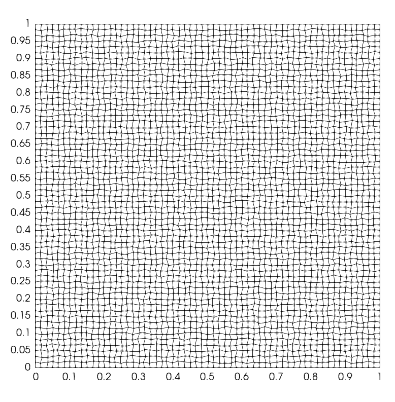
(a)

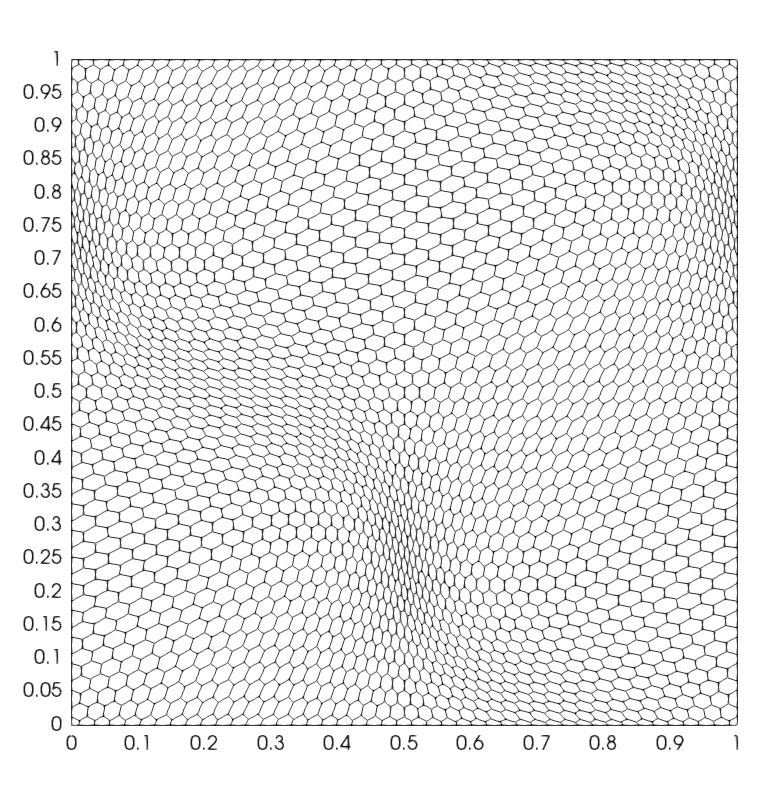
(b)

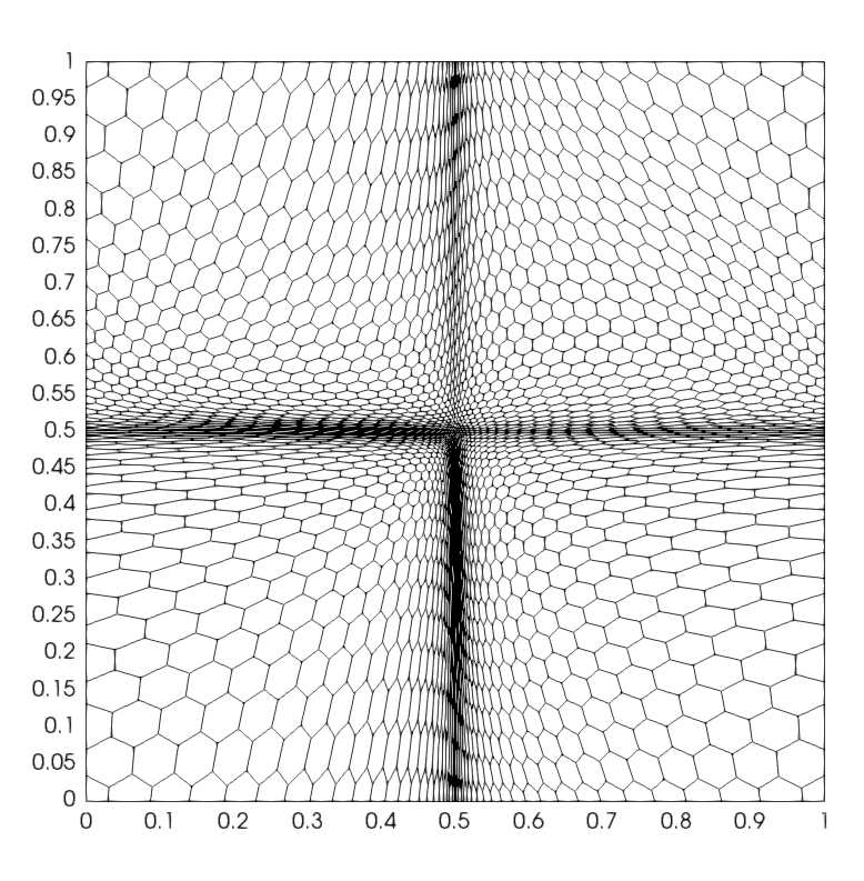
(c)

Figure 1: Meshes used in the numerical experiments. Left: Distorted squared mesh. Center: Distorted Voronoi mesh. Right: Highly-distorted Voronoi mesh.

In the second test, we compare the stabilization-free Virtual Element Method (SFVEM in short) with the standard VEM with the dofi-dofi stabilization term (VEM in short) [1] by plotting the relative errors $e_{0}$ and $e_{1}$ (5), and computing their rates of convergence on three families of distorted and highly-distorted meshes. The fourth refinement of each family of meshes is shown in Figure 1. In order to show the advantages of SFVEM with respect to the standard VEM, as suggested in [5], we consider an anisotropic diffusion tensor $\mathcal{K}$. Let $\Omega$ be the unit square, we consider the advection-diffusion-reaction problem (1) with coefficients

$$\mathcal{K}=\mathbf{G}\begin{bmatrix}1&0\\ 0&1.0e\text{-}09\end{bmatrix}\mathbf{G}^{T},\quad\mathbf{G}=\begin{bmatrix}\cos(\theta)&-\sin(\theta)\\ \sin(\theta)&\cos(\theta)\end{bmatrix},\quad\bm{\beta}(x,y)=\begin{bmatrix}\bm{\beta}_{1}(x,y)\\ \bm{\beta}_{2}(x,y)\end{bmatrix},$$

and $\gamma(x,y)=x(1-x)y(1-y)$, where $\mathbf{G}$ is the Givens rotation matrix with $\theta\in\mathbb{R}$. For $R_{1}$, $R_{2}\in[0,1]$, we define [3]

$$\bm{\beta}_{1}(x,y;R_{1}) =250000x^{4}y^{3}(R_{1}-x)(1-x)^{4}$$

$$\left[4R_{2}\left(1-5y+9y^{2}-7y^{3}+2y^{4}\right)-5y+24y^{2}-42y^{3}+32y^{4}-9y^{5}\right],$$

$$\bm{\beta}_{2}(x,y;R_{2}) =-\bm{\beta}_{1}(y,x;R_{2}),$$

and we fix $R_{1}=0.9$, $R_{2}=0.3$ and $\theta=\frac{\pi}{6}$. We choose $f(x,y)$ in such a way the exact solution is $u(x,y)=\bm{\beta}_{1}(x,y)$.

(a)

(b)

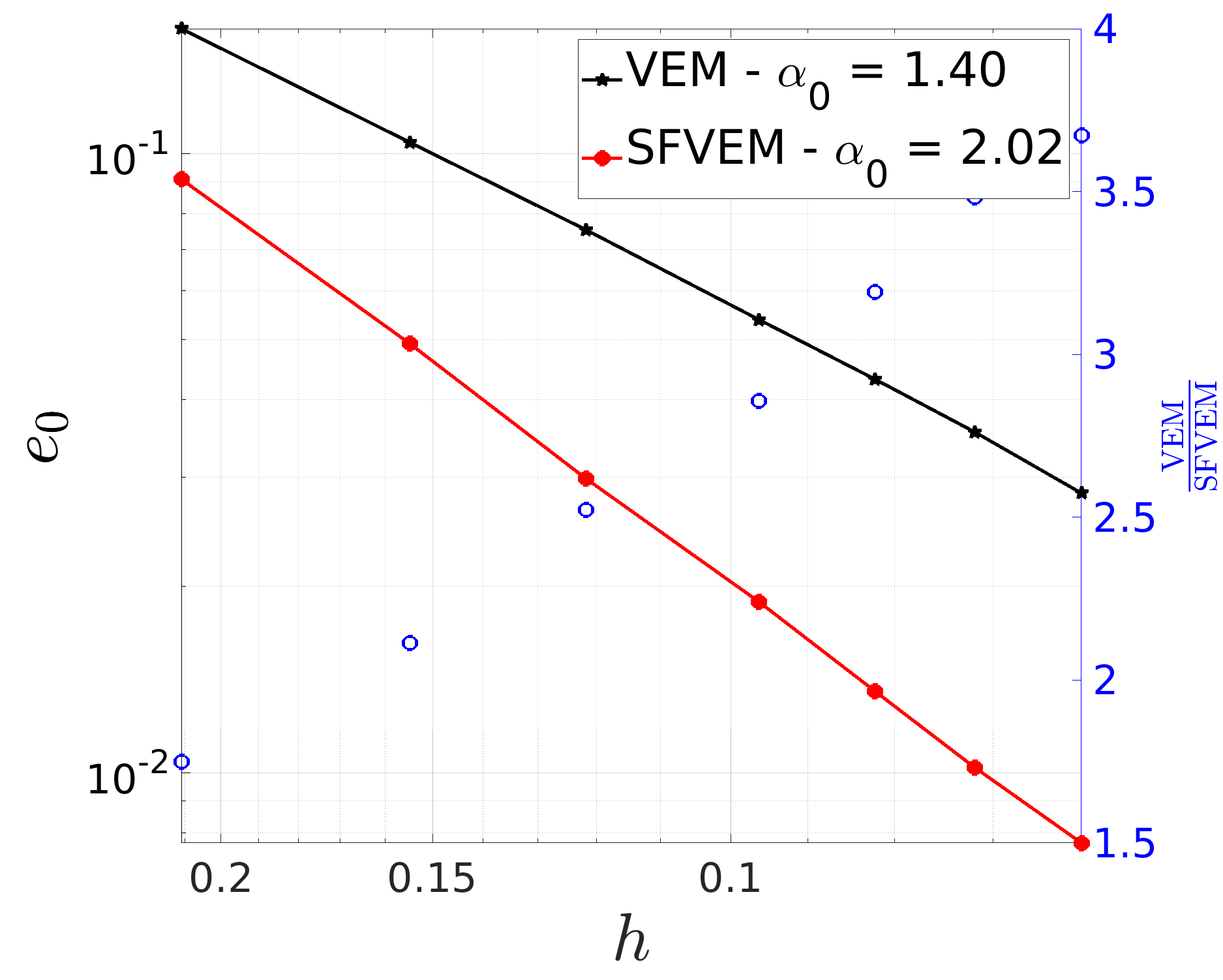
(c)

(d)

(e)

(f)

Figure 2: Behaviour of errors $e_{0}$ and $e_{1}$ (5) w.r.t. $h$. Left: Distorted squared mesh. Center: Distorted Voronoi mesh. Right: Highly-distorted Voronoi mesh.

In Figure 2, we plot the convergence curves of errors $e_{0}$ and $e_{1}$ (5) and the ratio between their values for VEM and SFVEM (right axis of each figure). The legends report the rates of convergence of the errors ($\alpha_{0}$ and $\alpha_{1}$, respectively). The performances of the two methods are almost equivalent concerning the $e_{1}$ error, see Figures 2(d)-2(f). Whereas in Figures 2(a)-2(c) SFVEM easily reaches the asymptotic rates of convergence on all the meshes and displays a smaller $e_{0}$ error, whereas VEM is still in a pre-asymptotic regime on highly-distorted Voronoi meshes and displays an error between two and three times w.r.t. SFVEM.

5 Conclusion

We propose a new first-order stabilization-free VEM that exploits projections on harmonic polynomials to build a self-stabilized bilinear form. Numerical results show good stability of the method and optimal rates of convergence.

References

• [1] L. Beirão da Veiga, F. Brezzi, L. D. Marini, and A. Russo. Virtual element methods for general second order elliptic problems on polygonal meshes. Math. Models Methods Appl. Sci., 26(04):729–750, 2015.
• [2] L. Beirão da Veiga and G. Manzini. Residual a posteriori error estimation for the virtual element method for elliptic problems. ESAIM: M2AN, 49(2):577–599, 2015.
• [3] S. Berrone. Robustness in a posteriori error estimates for the oseen equations with general boundary conditions. In Numerical Mathematics and Advanced Applications, pages 657–668. Springer Milan, 2003.
• [4] Stefano Berrone, Andrea Borio, and Francesca Marcon. Lowest order stabilization free Virtual Element Method for the Poisson equation, 2021.
• [5] Stefano Berrone, Andrea Borio, and Francesca Marcon. Comparison of standard and stabilization free Virtual Elements on anisotropic elliptic problems. App. Math. Lett., 129:107971, 2022.
• [6] J. Blair Perot and Chris Chartrand. A mimetic method for polygons. J. Comput. Phys., 424(C):109853, 2021.