Local Exact-Diffusion for Decentralized Optimization and Learning

Abstract

Distributed optimization methods with local updates have recently attracted a lot of attention due to their potential to reduce the communication cost of distributed methods. In these algorithms, a collection of nodes performs several local updates based on their local data, and then they communicate with each other to exchange estimate information. While there have been many studies on distributed local methods with centralized network connections, there has been less work on decentralized networks.

In this work, we propose and investigate a locally updated decentralized method called Local Exact-Diffusion (LED). We establish the convergence of LED in both convex and nonconvex settings for the stochastic online setting. Our convergence rate improves over the rate of existing decentralized methods. When we specialize the network to the centralized case, we recover the state-of-the-art bound for centralized methods. We also link LED to several other independently studied distributed methods, including Scaffnew, FedGate, and VRL-SGD. Additionally, we numerically investigate the benefits of local updates for decentralized networks and demonstrate the effectiveness of the proposed method.

1 Introduction

This work examines the distributed consensus optimization problem, as formally presented in (2). In this setup, a network of nodes (also referred to as agents, workers, or clients) collaboratively seeks to minimize the average of the nodes’ objectives. This formulation is appealing for large scale data problems because it is more efficient to use distributed solution methods to reduce the computational burden for large data sets. In terms of communication protocol, distributed methods can be classified as either centralized or decentralized. Centralized distributed methods require all nodes to communicate with a central server (e.g., server-workers connection) without sharing private data, as seen in parallel optimization [1] and federated learning [2, 3]. In this setup, there is a central node that is responsible for aggregating local variables and updating model estimates. In contrast, decentralized distributed methods are “fully distributed” that are designed for arbitrary connected network topologies such as line, ring, grid, and random graphs. These methods require nodes to communicate only with their immediate neighbors [4, 5]. It’s important to note that decentralized methods can adapt to a centralized setting when the network is fully connected.

In this paper, we consider a group of $N$ nodes, connected via an undirected decentralized network, collaborating to solve the optimization problem:

$$\begin{array}[]{ll}\min\limits_{x\in{}^{m}}&f(x)\triangleq\displaystyle\frac{1}{N}\sum\limits_{i=1}^{N}f_{i}(x),\quad f_{i}(x)\triangleq\mathop{\mathbb{E}{}}[F_{i}(x;\xi_{i})],\end{array}$$ (2)

where $f_{i}:{}^{m}\rightarrow\real$ ($i=1,\dots,N$) represents a smooth function known only to node $i$. This function is defined as the expected value of some loss function $F_{i}(\cdot;\xi_{i})$ over the random variable or data $\xi_{i}$. We focus on the stochastic online setting, in which each node has access only to random samples of its data $\{\xi_{i}\}$. Problems of the form (2) have received a lot of attention in control and engineering communities [4, 6, 7, 8], as well as in the machine learning community [9, 10, 11] .

Our main contribution is the proposal and study of a local variant of the decentralized Exact-Diffusion algorithm [12, 13] (see also [6]), where nodes employ multiple local updates between communication rounds. We establish the algorithm’s convergence in both convex and nonconvex settings. . Our bounds improve upon those of decentralized methods and match the best known results for centralized methods. Before we formally state our contributions, we will first discuss some related works.

1.1 Related works

We begin by discussing relevant centralized methods, which require a central server for implementation. One of the most popular centralized methods is FedAvg, which involves a random subset of nodes performing multiple local stochastic gradient descent (SGD) updates at each round; They then send their estimates (parameters) to the central server, which averages these estimates and sends them back to replace the local estimates [3]. It should be noted that FedAvg is often called Local-SGD. Several works have analyzed FedAvg and Local-SGD [14, 15, 16, 17, 18, 19]. It has been observed that the performance of FedAvg and Local-SGD is suboptimal for heterogeneous data and that an increased number of local steps can lead to worse performance [20]. One major reason is that node estimates drift toward their local solutions due to local updates, resulting in a biased solution [18, 19, 10]. To correct this drift in FedAvg and Local-SGD, several algorithms have been proposed, including SCAFFOLD [10], FedDyn [21], FedPD [22], VRL-SGD [23], and FedGATE [24]. These methods, however, are only applicable to centralized connections.

In this work, we focus on decentralized setups as presented in [5, 4]. The most extensively studied method for this setup is the decentralized stochastic gradient descent method (DSGD) [25, 26, 8, 9, 17, 11]. The study in [9] showcased that DSGD achieves the centralized SGD rate asymptotically, a distributed trait termed as linear speedup [28]. However, DSGD converges to a biased solution, and this bias is further negatively influenced by network sparsity [13, 11]. The bias arises from the heterogeneity among the local functions ${f_{i}}$, as characterized by $(1/N)\sum_{i=1}^{N}\|{\nabla}f_{i}(x)-{\nabla}f(x)\|^{2}$. This value, which is required to be bounded for the analysis of DSGD [9, 11], can become quite large when the functions are heterogeneous, thereby slowing down the convergence of DSGD [13, 29]. Multiple studies have introduced bias-correction algorithms resistant to local function heterogeneity, such as the alternating direction method of multipliers (ADMM) based methods [30, 31], EXTRA [32], Exact-Diffusion (ED) [12, 13] (also known as NIDS [33] and D² [34]), and Gradient-Tracking (GT) methods [35, 36, 37, 38]. It has been established that these bias-correction methods outperform DSGD [29]. Yet, all these methods necessitate communication at every iteration.

Locally updated stochastic decentralized methods have received less attention than centralized methods and are more challenging to study. Federated learning can be viewed as a subset of decentralized optimization and learning under time-varying and asynchronous updates [39]. For instance, DSGD with local steps, termed Local-DSGD, has been studied in [40, 41, 11, 17] and is analogous to Local-SGD when the network is fully connected. However, just as DSGD suffers from bias, Local-DSGD does too. Furthermore, similar to Local-SGD, it also experiences drift. Increasing the number of local steps exacerbates this drift in the solution, requiring the use of very small stepsizes, which significantly slows down convergence.

Only a few works have studied decentralized methods with local updates and bias correction. The work in [42] studied Local Gradient-Tracking (LGT) under nonconvex costs, but it focused solely on deterministic settings. Similarly, the research presented in [43] explored a locally updated stochastic variant of gradient-tracking, namely $K$-GT, but it too addressed only nonconvex settings. In this paper, we propose and investigate a different algorithm inspired by [12, 6]. Our results improve upon the rates of local GT-based methods and require just half the communication cost of existing approaches. Furthermore, our rates surpass those of Local-DSGD [11, 17]. Importantly, when employing a constant step size, LED achieves precise convergence in the deterministic (noiseless) case. In contrast, Local-DSGD does not, due to the bias/drift introduced by the heterogeneity in local functions, as discussed earlier. We will next formally outline our contributions.

1.2 Contribution

• We propose Local Exact-Diffusion (LED) method for distributed optimization with local updates. An advantage over previous methods is that LED is a decentralized method that only requires one single vector communication per link and is robust to the functions heterogeneity – See Table 1. Numerical results are provided to demonstrate the effectiveness of LED over other methods.

• We provide insights and draw connections between our proposed method and the following state-of-the-art algorithms: Exact-Diffusion [12], NIDS [33], D² [34], ProxSkip/Scaffnew [44], VRL-SGD [23], and FedGATE [24]. For instance, we demonstrate that LED can be interpreted as Scaffnew [44] with fixed local updates instead of random ones. We also show that LED is a decentralized variant of the centralized methods FedGATE [24] and VRL-SGD [23]. Furthermore, we highlight that all these methods can be traced back to the primal-dual method PDFP2O [45] (also known as PAPC [46]) in the case of a single local update.

• We establish the convergence of LED in both (strongly-)convex and nonconvex environments for online stochastic learning settings. Our rates improve upon existing bounds for local decentralized methods—see Table 2. It is worth noting that the analysis of LED is more challenging than that of Local-DSGD, even in the single local update scenario. Additionally, in contrast to Local-DSGD, LED is robust to heterogeneity in local functions and converges exactly in the deterministic case (no noise), as discussed earlier.

  A byproduct of our result is that, when adapting our analysis to centralized networks, we achieve new and tighter analyses for the methods VRL-SGD [23] and FedGATE [24].

Table 1: Differences with existing methods employing local steps.

Method Decentralized Single communication Robust to functions heterogeneity SCAFFOLD [10] $\bm{\times}$ $\bm{\times}$ ✓ VRL-SGD [23]/FedGate [24] $\bm{\times}$ ✓ ✓ Local-DSGD [11] ✓ ✓ $\bm{\times}$ LGT [42] and $K$-GT [43] ✓ $\bm{\times}$ ✓ LED [this work] ✓ ✓ ✓

Notation. Lowercase letters represent vectors and scalars, while uppercase letters denote matrices. The notation $\mathrm{col}\{a_{1},\ldots,a_{n}\}$ (or $\mathrm{col}\{a_{i}\}_{i=1}^{n}$) stands for the vector that stacks the vectors (or scalars) $a_{i}$ on top of each other. We use ${\rm diag}\{d_{1},\ldots,d_{n}\}$ (or ${\rm diag}\{d_{i}\}_{i=1}^{n}$) to represent a diagonal matrix with the diagonal elements $d_{i}$. Additionally, the symbol ${\rm blkdiag}\{D_{1},\ldots,D_{n}\}$ (or ${\rm blkdiag}\{D_{i}\}_{i=1}^{n}$) denotes a block diagonal matrix with diagonal blocks $D_{i}$. The notations $\mathbf{1}$ and $\mathbf{0}$ represent vectors of all ones and zeros, respectively. The dimension is determined from the context, or we use notation like $\mathbf{1}_{n}$. The inner product of two vectors $a$ and $b$ is given by $\langle a,b\rangle$. The symbol $\otimes$ indicates the Kronecker product operation. We use upright bold symbols, such as ${\mathbf{x}},{\mathbf{f}},{\mathbf{W}}$, to represent augmented network quantities.

Outline. This paper is organized as follows: Section 2 introduces our algorithm and its motivation. In Section 3, we compare our method with other leading approaches. Section 4 presents our core assumptions and convergence findings, and a discussion comparing our results with prior works. Section 5 provides simulation outcomes, and conclusions are drawn in Section 6. Detailed proofs are reserved for the appendix.

2 Local Exact-Diffusion

In this section, we start by describing the proposed algorithm in its decentralized implementation. We then rewrite it in network notation for reasons of analysis and interpretation.

2.1 Algorithm description

The method under study is described in Alg. 1 and is named Local Exact-Diffusion (LED). In step 1, each node $i$ employs $\uptau$ local updates, starting from the initialization $x_{i}^{r}$, which is its local estimate of the solution after the communication round $r$. Step 2 is the communication round during which each node $i$ sends its local intermediate estimate $\phi_{i,\uptau}^{r}$ to its neighbors $j\in{\mathcal{N}}_{i}$, where the symbol ${\mathcal{N}}_{i}$ denotes the set of neighbors of node $i$ (including node $i$); in this step, $w_{ij}$ is a nonnegative scalar weight that node $i$ uses to scale the information received from node $j\in{\mathcal{N}}_{i}$. The final step, step 3, is where each node $i$ updates its (dual) estimate $y_{i}^{r}\in{}^{m}$.

Algorithm 1 Local Exact-Diffusion (LED)

node $i$ input: $x_{i}^{0}$, $\alpha>0$, $\beta>0$, and $\uptau$.

initialize $y_{i}^{0}=x_{i}^{0}-\sum_{j\in{\mathcal{N}}_{i}}w_{ij}x_{j}^{0}$ (or $y_{i}^{0}=0$).

repeat for $r=0,1,2,\dots$

1. Local primal updates: set $\phi_{i,0}^{r}=x_{i}^{r}$ and do $\uptau$ local updates:

   $$\phi_{i,t+1}^{r} =\phi_{i,t}^{r}-\alpha{\nabla}F_{i}(\phi_{i,t}^{r};\xi_{i,t}^{r})-\beta y_{i}^{r},\quad t=0,\dots,\uptau-1.$$ (3a)

2. Diffusion:

   $$x_{i}^{r+1} =\sum_{j\in{\mathcal{N}}_{i}}w_{ij}\phi_{j,\uptau}^{r}.$$ (3b)

3. Local dual update:

   $$y_{i}^{r+1} =y_{i}^{r}+\phi_{i,\uptau}^{r}-x_{i}^{r+1}.$$ (3c)

2.2 Networked description

The LED method, as listed in 1, is described at the node level. For the analysis and interpretation of the method, we will present it in a networked form. To do this, we introduce the following network weight matrix notation:

$$W\triangleq[w_{ij}]\in{}^{N\times N},\quad{\mathbf{W}}\triangleq W\otimes I_{m}\in{}^{mN\times mN}.$$ (4)

Using the above notation, we have ${\mathbf{W}}{\mathbf{u}}=\mathrm{col}\{\sum_{j\in{\mathcal{N}}_{i}}w_{ij}u_{j}\}_{i=1}^{N}$ for any vector ${\mathbf{u}}$ with the structure ${\mathbf{u}}=\mathrm{col}\{u_{1},\dots,u_{N}\}$, where $u_{i}\in{}^{m}$ [27]. Thus, if we introduce the augmented network quantities:

$${\mathbf{x}}^{r} \triangleq\mathrm{col}\{x_{1}^{r},\dots,x_{N}^{r}\}\in{}^{mN}$$ (5a)

$$\bm{\Phi}^{r}_{t} \triangleq\mathrm{col}\{\phi_{1,t}^{r},\dots,\phi_{N,t}^{r}\}\in{}^{mN}$$ (5b)

$${\mathbf{y}}^{r} \triangleq\mathrm{col}\{y_{1}^{r},\dots,y_{N}^{r}\}\in{}^{mN}$$ (5c)

$${\mathbf{f}}({\mathbf{x}}) \triangleq\sum_{i=1}^{N}f_{i}(x_{i})$$ (5d)

$${\nabla}{\mathbf{f}}({\mathbf{x}}) \triangleq\mathrm{col}\{{\nabla}f_{1}(x_{1}),\dots,{\nabla}F_{N}(x_{N})\}\in{}^{mN}$$ (5e)

$${\nabla}{\mathbf{F}}({\mathbf{x}};\bm{\xi}) \triangleq\mathrm{col}\{{\nabla}F_{1}(x_{1};\xi_{1}),\dots,{\nabla}F_{N}(x_{N};\xi_{N})\}\in{}^{mN}.$$ (5f)

Then, Algorithm 1 can be represented in a compact networked form as follows: Given ${\mathbf{x}}^{0}$, set ${\mathbf{y}}^{0}=({\mathbf{I}}-{\mathbf{W}}){\mathbf{x}}^{0}$ (or ${\mathbf{y}}^{0}=\mathbf{0}$) and update for $r=0,1,2,\dots$

1. Local primal updates: set $\bm{\Phi}_{0}^{r}={\mathbf{x}}^{r}$, for $t=0,\dots,\uptau-1$:

   $$\bm{\Phi}^{r}_{t+1} =\bm{\Phi}^{r}_{t}-\alpha{\nabla}{\mathbf{F}}(\bm{\Phi}^{r}_{t};\bm{\xi}_{t}^{r})-\beta{\mathbf{y}}^{r}.$$ (6a)

2. Diffusion round:

   $${\mathbf{x}}^{r+1} ={\mathbf{W}}\bm{\Phi}^{r}_{\uptau}.$$ (6b)

3. Local dual update:

   $${\mathbf{y}}^{r+1} ={\mathbf{y}}^{r}+({\mathbf{I}}-{\mathbf{W}})\bm{\Phi}^{r}_{\uptau}.$$ (6c)

The networked description (6) will be used for analysis purposes.

2.3 Motivation and relation with Exact-Diffusion

Exact-Diffusion (ED) was derived in [12] and takes the following form:

$${\mathbf{x}}^{r+1} ={\mathbf{W}}\big{(}2{\mathbf{x}}^{r}-{\mathbf{x}}^{r-1}-\alpha({\nabla}{\mathbf{f}}({\mathbf{x}}^{r})-{\nabla}{\mathbf{f}}({\mathbf{x}}^{r-1}))\big{)}.$$ (7)

The unified decentralized algorithm (UDA) from [6] demonstrated that the iterates ${\mathbf{x}}^{r}$ of ED in (7) can be equivalently described by:

UDA-ED $$\bm{\Phi}^{r}={\mathbf{x}}^{r}-\alpha{\nabla}{\mathbf{f}}({\mathbf{x}}^{r})-{\mathbf{B}}^{1/2}{\mathbf{z}}^{r}$$ (8a)

UDA-ED $${\mathbf{x}}^{r+1}={\mathbf{W}}\bm{\Phi}^{r}$$ (8b)

UDA-ED $${\mathbf{z}}^{r+1}={\mathbf{z}}^{r}+{\mathbf{B}}^{1/2}\bm{\Phi}^{r},$$ (8c)

where ${\mathbf{B}}={\mathbf{I}}-{\mathbf{W}}$. The above form is convenient for analytical purposes; however, it cannot be implemented in a decentralized fashion due to ${\mathbf{B}}^{1/2}=({\mathbf{I}}-{\mathbf{W}})^{1/2}$.

To derive our method, we set ${\mathbf{B}}=\beta({\mathbf{I}}-{\mathbf{W}})$ in (8c) and introduce the change of variable ${\mathbf{y}}^{r}=\frac{1}{\beta}{\mathbf{B}}^{1/2}{\mathbf{z}}^{r}$. This leads to the following description:

LED-1 $$\bm{\Phi}^{r}={\mathbf{x}}^{r}-\alpha{\nabla}{\mathbf{f}}({\mathbf{x}}^{r})-\beta{\mathbf{y}}^{r}$$ (9a)

LED-1 $${\mathbf{x}}^{r+1}={\mathbf{W}}\bm{\Phi}^{r}$$ (9b)

LED-1 $${\mathbf{y}}^{r+1}={\mathbf{y}}^{r}+({\mathbf{I}}-{\mathbf{W}})\bm{\Phi}^{r}.$$ (9c)

It can be observed that the update LED-1 (9c) is equivalent to LED (6) when $\uptau=1$. In other words, LED (6) is an extension of LED-1 (9c) that incorporates local updates.

Remark 1 (NIDS, and D²).

The NIDS method from [33] is given by

$${\mathbf{x}}^{r+1}=\widetilde{{\mathbf{W}}}\left(2{\mathbf{x}}^{r}-{\mathbf{x}}^{r-1}-\alpha\left(\nabla{\mathbf{f}}({\mathbf{x}}^{r})-\nabla{\mathbf{f}}({\mathbf{x}}^{r-1})\right)\right),$$

where $\widetilde{{\mathbf{W}}}=(1-\alpha c){\mathbf{I}}+\alpha c{\mathbf{W}}$ and $c$ is a stepsize parameter. When $c=1/\alpha$, NIDS reduces to ED (7). We also note that ED (or NIDS with $c=1/\alpha$) has been studied under the name D² [34]. Thus, LED can be viewed as a modification of NIDS/D² that incorporates local updates. $\blacksquare$

Remark 2 (Non-Equivalence with Local Updates).

It is important to note that the updates (7), (8c), and (9c) are equivalent only when there are no multiple local updates and $\beta=1$. To understand this, observe that the local updates variants can be modeled as a time-varying graph ${\mathbf{W}}_{r}$, where ${\mathbf{W}}_{r}={\mathbf{W}}$ when $r=\uptau,2\uptau,3\uptau,\dots$, and ${\mathbf{W}}_{k}={\mathbf{I}}$ otherwise. In this scenario, the updates ${\mathbf{x}}^{r}$ differ for all these methods. Indeed, for this case, the updates (7) and (8c) are not guaranteed to converge and often diverge in simulations. $\blacksquare$

3 Connection with existing algorithms

In this section, we discuss and highlight the connections of LED to the following algorithms: Scaffnew/ProxSkip [44], VRL-SGD [23], and FedGate [24]. We also demonstrate that all these methods can be traced back to the primal-dual method PDFP2O [45], which is also known as PAPC [46] and was initially proposed in [47] for quadratic objectives.

3.1 Relation with PDFP2O/PAPC

We now demonstrate that LED (6) with $\uptau=1$ (i.e., LED-$1$ (9c)) can be interpreted as the primal-dual algorithm PDFP2O [45] applied to the following reformulation of problem (2):

$$\min_{{\mathbf{x}}}\quad{\mathbf{f}}({\mathbf{x}})+{\mathbf{g}}({\mathbf{B}}^{1\over 2}{\mathbf{x}}),$$ (10)

where ${\mathbf{B}}={\mathbf{I}}-{\mathbf{W}}$ and ${\mathbf{g}}$ is the indicator function of zero, i.e., ${\mathbf{g}}({\mathbf{u}})=0$ if ${\mathbf{u}}=\mathbf{0}$ and $g({\mathbf{u}})=+\infty$ otherwise. Problem (10) is equivalent to (2) because ${\mathbf{B}}{\mathbf{x}}=\mathbf{0}$ if and only if $x_{1}=x_{2}=\dots=x_{N}$ – see [32, 48].

The following updates are obtained when PDFP2O [45] is applied to formulation (10):

PDFP2O $${\mathbf{v}}^{r+1}=\operatorname{prox}_{\frac{\alpha}{\eta}{\mathbf{g}}^{*}}\left({\mathbf{B}}^{1\over 2}({\mathbf{x}}^{r}-\alpha\nabla{\mathbf{f}}({\mathbf{x}}^{r}))+\left({\mathbf{I}}-\eta{\mathbf{B}}\right){\mathbf{v}}^{r}\right)$$ (11a)

PDFP2O $${\mathbf{x}}^{r+1}={\mathbf{x}}^{r}-\alpha\nabla{\mathbf{f}}({\mathbf{x}}^{r})-\eta{\mathbf{B}}^{1\over 2}{\mathbf{v}}^{r+1},$$ (11b)

where $\operatorname{prox}_{\frac{\alpha}{\eta}{\mathbf{g}}^{*}}(\cdot)$ denotes the proximal operator of the conjugate of $g$ and $\alpha,\eta>0$ are stepsize parameters. The following result relates LED-1 (9c) (LED (6) with $\uptau=1$) with PDFP2O (11b).

Proposition 1 (Relation to PDFP2O).

The updates of PDFP2O (11b) can be rewritten as

$$\bm{\Phi}^{r} =\mathbf{x}^{r}-\alpha{\nabla}\mathbf{f}(\mathbf{x}^{r})-\eta{\mathbf{y}}^{r}$$ (12a)

$$\mathbf{y}^{r+1} =\mathbf{y}^{r}+({\mathbf{I}}-{\mathbf{W}})\bm{\Phi}^{r}$$ (12b)

$$\mathbf{x}^{r+1} =\left((1-\eta){\mathbf{I}}+\eta{\mathbf{W}}\right)\bm{\Phi}^{r}.$$ (12c)

It follows that PDFP2O (12) is equivalent to LED-1 (9c) when $\eta=\beta=1$.

Proof.

If we let $\bm{\Phi}^{r}=\mathbf{x}^{r}-\alpha{\nabla}\mathbf{f}(\mathbf{x}^{r})-\eta\mathbf{B}^{1\over 2}\mathbf{v}^{r}$, then we can rewrite equation (11b) as follows:

$$\bm{\Phi}^{r} =\mathbf{x}^{r}-\alpha{\nabla}\mathbf{f}(\mathbf{x}^{r})-\eta\mathbf{B}^{1\over 2}\mathbf{v}^{r}$$ (13a)

$$\mathbf{v}^{r+1} =\operatorname{prox}_{\frac{\alpha}{\eta}{\mathbf{g}}^{*}}\left(\mathbf{v}^{r}+\mathbf{B}^{1\over 2}\bm{\Phi}^{r}\right)$$ (13b)

$$\mathbf{x}^{r+1} =\mathbf{x}^{r}-\alpha{\nabla}\mathbf{f}(\mathbf{x}^{r})-\eta\mathbf{B}^{1\over 2}\mathbf{v}^{r+1}.$$ (13c)

Since ${\mathbf{g}}$ is the indicator function of zero, we have $\operatorname{prox}_{\frac{\alpha}{\eta}{\mathbf{g}}^{*}}({\mathbf{z}})={\mathbf{z}}$; thus $\mathbf{v}^{r+1}=\mathbf{v}^{r}+\mathbf{B}^{1\over 2}\bm{\Phi}^{r}$. Moreover, observe that

$$\mathbf{x}^{r+1} =\mathbf{x}^{r}-\alpha{\nabla}\mathbf{f}(\mathbf{x}^{r})-\eta\mathbf{B}^{1\over 2}\mathbf{v}^{r+1}$$

$$=\mathbf{x}^{r}-\alpha{\nabla}\mathbf{f}(\mathbf{x}^{r})-\eta\mathbf{B}^{1\over 2}\mathbf{v}^{r}-\eta\mathbf{B}^{1\over 2}(\mathbf{v}^{r+1}-\mathbf{v}^{r})$$

$$=\bm{\Phi}^{r}-\eta{\mathbf{B}}\bm{\Phi}^{r}=({\mathbf{I}}-\eta{\mathbf{B}})\bm{\Phi}^{r}.$$

Therefore, (13) can be represented as:

$$\bm{\Phi}^{r} =\mathbf{x}^{r}-\alpha{\nabla}\mathbf{f}(\mathbf{x}^{r})-\eta\mathbf{B}^{1\over 2}\mathbf{v}^{r}$$

$$\mathbf{v}^{r+1} =\mathbf{v}^{r}+\mathbf{B}^{1\over 2}\bm{\Phi}^{r}$$

$$\mathbf{x}^{r+1} =({\mathbf{I}}-\eta{\mathbf{B}})\bm{\Phi}^{r}.$$

Introducing ${\mathbf{y}}^{r}=\mathbf{B}^{1\over 2}\mathbf{v}^{r}$ and using ${\mathbf{B}}={\mathbf{I}}-{\mathbf{W}}$, the above updates can be rewritten as given in (12). Recall that when $\uptau=1$, we can remove the subscript $t$ from $\bm{\Phi}^{r}_{t}$ and describe the updates (6) as given in (9c). When $\eta=\beta=1$, the updates (12) and (9c) are identical. ∎

Remark 3 (ED, NIDS, and D² interpretations).

The above result demonstrates that LED (6) can be interpreted as a locally updated variant of PDFP2O (11b). It also shows that ED/D² [12, 34] and NIDS [33] are different representations of PDFP2O [45] applied on formulation (10). $\blacksquare$

3.2 Relation with Scaffnew

The work [44] studied a proximal skipping variant of PDFP2O. The decentralized Scaffnew method is given by [44, Alg. 5]:

$$\bm{\Phi}^{r}={\mathbf{x}}^{r}-\alpha\left(\nabla{\mathbf{f}}\left({\mathbf{x}}^{r}\right)+{\mathbf{z}}^{r}\right).$$ (15a)

Generate a random number $$\theta_{t}\in\{0,1\} \operatorname{Prob}\left(\theta_{t}=1\right)=p$$ with and update:

$$\begin{cases}{\mathbf{x}}^{r+1}=(1-\frac{\alpha\zeta}{p})\bm{\Phi}^{r}+\frac{\alpha\zeta}{p}{\mathbf{W}}\bm{\Phi}^{r},\\ {\mathbf{z}}^{r+1}={\mathbf{z}}^{r}+\frac{p}{\alpha}(\bm{\Phi}^{r}-{\mathbf{x}}^{r+1})={\mathbf{z}}^{r}+\zeta({\mathbf{I}}-{\mathbf{W}})\bm{\Phi}^{r}&\text{ if }\theta_{t}=1\\ {\mathbf{x}}^{r+1}=\bm{\Phi}^{r},\\ {\mathbf{z}}^{r+1}={\mathbf{z}}^{r}&\text{otherwise},\end{cases}$$ (15b)

where $\alpha,\zeta$ are stepsize parameters. Observe that (15) employs local updates (15a) and communicates only with a small probability $p$ (15b). If we let ${\mathbf{y}}^{r}=(1/\zeta){\mathbf{z}}^{r}$ and $p=1$ (communicate at each iteration) then (15) reduces to

$$\bm{\Phi}^{r} ={\mathbf{x}}^{r}-\alpha\nabla{\mathbf{f}}\left({\mathbf{x}}^{r}\right)-\alpha\zeta{\mathbf{y}}^{r}$$ (16a)

$${\mathbf{x}}^{r+1} =\left((1-\alpha\zeta){\mathbf{I}}+\alpha\zeta{\mathbf{W}}\right)\bm{\Phi}^{r},$$ (16b)

$${\mathbf{y}}^{r+1} ={\mathbf{y}}^{r}+({\mathbf{I}}-{\mathbf{W}})\bm{\Phi}^{r}.$$ (16c)

The update (16) is the same as PDFP2O (12) when $\eta=\alpha\zeta$. Consequently, when $p=1$ and $\zeta=1/\alpha$ (16) is exactly LED-1 (9c) when $\beta=1$.

Remark 4.

LED (6) employs a fixed number $\uptau$ of local updates between two communication rounds, whereas Scaffnew uses random number of local updates between two communication rounds. The use of random communication skipping or fixed local steps differs in analysis, however, in terms of performance they are strikingly similar with $1/p$ playing the role of $\uptau$.

The work [44] analyzes Scaffnew and shows that local steps can save communication when the network is well connected. We point out that the analysis techniques in [44] do not show linear speedup and are only-suited for the probabilistic implementation with strongly-convex costs. The techniques we present in this work are distinct and applicable to the locally updated variant with a deterministic number of local updates (6) for both nonconvex and (strongly-)convex settings. $\blacksquare$

3.3 Relation with FedGATE/VRL-SGD

The work [24] introduced and analyzed a federated learning algorithm (centralized method) named FedCOMGATE that employs compression; without compression the method reduces to FedGATE [24, Alg. 3], which is a generalization of VRL-SGD [23]. We will now show the relationship between FedGATE/VRL-SGD and the centralized version of LED. As a first step, we will represent FedGATE/VRL-SGD in a networked form.

FedGATE is described as follows [24, Alg. 3]: For $r=0,1,2,\dots$, set $\phi_{i,0}^{r}=x^{r}$, for $t=0,\dots,\uptau-1$:

$$\phi_{i,t+1}^{r} =\phi_{i,t}^{r}-\alpha({\nabla}F_{i}(\phi_{i,t}^{r};\xi_{i,t}^{r})-\delta_{i}^{r}),\quad t=0,\dots,\uptau-1.$$ (17a)

Update

$$\delta_{i}^{r+1} =\delta_{i}^{r}-\frac{1}{\alpha\uptau}\left(\phi_{i,\uptau}^{r}-\frac{1}{N}\sum_{j=1}^{N}\phi_{j,\uptau}^{r}\right)$$ (17b)

$$x^{r+1} =x^{r}-\alpha\gamma\big{(}x^{r}-\frac{1}{N}\sum_{j=1}^{N}\phi_{j,\uptau}^{r}\big{)},$$ (17c)

where $\gamma$ is a global stepsize parameter. By letting $y_{i}^{r}=-\alpha\uptau\delta_{i}^{r}$ and employing the network notation defined in (5) with ${\mathbf{x}}^{r}=\mathbf{1}\otimes x^{r}$, the method above can be rewritten as:

$$\bm{\Phi}^{r}_{t+1} =\bm{\Phi}^{r}_{t}-\alpha{\nabla}{\mathbf{F}}(\bm{\Phi}^{r}_{t};\bm{\xi}_{t}^{r})-\frac{1}{\uptau}{\mathbf{y}}^{r},\quad t=0,\dots,\uptau-1.$$ (18a)

Then update

$${\mathbf{x}}^{r+1} =(1-\alpha\gamma){\mathbf{x}}^{r}+\alpha\gamma(\tfrac{1}{N}\mathbf{1}\mathbf{1}^{\textit{\footnotesize{T}}})\bm{\Phi}^{r}_{\uptau}$$ (18b)

$${\mathbf{y}}^{r+1} ={\mathbf{y}}^{r}+({\mathbf{I}}-\tfrac{1}{N}\mathbf{1}\mathbf{1}^{\textit{\footnotesize{T}}})\bm{\Phi}^{r}_{\uptau}.$$ (18c)

It’s now evident that when $\alpha\gamma=1$, the update (18) aligns with LED (6) when ${\mathbf{W}}=\tfrac{1}{N}\mathbf{1}\mathbf{1}^{\textit{\footnotesize{T}}}$ and $\beta=1/\uptau$. It’s worth noting that the updates (18) simplify to VRL-SGD [23] when $\alpha\gamma=1$ [24]. In essence, FedGATE with $\alpha\gamma=1$ (or VRL-SGD) corresponds to LED in the fully connected network scenario. This also suggests that FedGATE and VRL-SGD are locally updated versions of PDFP2O (11b) with ${\mathbf{B}}={\mathbf{I}}-\tfrac{1}{N}\mathbf{1}\mathbf{1}^{\textit{\footnotesize{T}}}$.

Remark 5 (Equivalence).

All of the derivations in this section require appropriate stepsizes tuning and are based on the assumption that the graph is static (i.e., $W$ is constant). When the stepsizes differ or the graph is dynamic (as in the local update variant), these various representation may not necessarily be equivalent. We note that the analysis techniques from [12, 6] are particularly suited for static graphs and are limited to the strongly-convex case. Moreover, the techniques from [23, 24] are tailored for centralized networks. In contrast, our analyses address the more challenging decentralized connections with local updates; thus, our techniques can be specialized for these methods. In fact, our analysis can provide tighter rates compared to those in [23, 24]. Remark 8 explains how to adapt our techniques to the centralized scenario.

4 Convergence result

In this section, we present our main convergence findings and discuss how they differ from previous results. Before proceeding, we will review the assumptions necessary for our results to hold, which are standard in the literature [29, 23, 24].

4.1 Assumptions

Assumption 1 (Weight matrix).

The weight matrix $W$ is symmetric, doubly stochastic, and primitive. Moreover, we assume that $W$ is positive definite. $\blacksquare$

Under Assumption 1, the eigenvalues of $W$, denoted by $\{\lambda_{i}\}_{i=1}^{N}$, are all strictly less than one (in magnitude for nonpositive definite $W$), with the exception of a single eigenvalue at one, which we denote by $\lambda_{1}$. The network’s mixing rate is defined as:

$$\lambda\triangleq\left\|W-\tfrac{1}{N}\mathbf{1}\mathbf{1}^{\textit{\footnotesize{T}}}\right\|=\max_{i\in\{2,\ldots,N\}}|\lambda_{i}|<1.$$ (19)

We remark that the positive definiteness assumption can be easily satisfied because, given a symmetric doubly stochastic matrix $\tilde{W}$, we can construct a positive definite weight matrix by $W=0.5(\tilde{W}+I)$.

Assumption 2 (Bounded variance).

Each stochastic gradient ${\nabla}F_{i}(x_{i}^{k};\xi_{i}^{k})$ is unbiased with bounded variance:

$$\textstyle\mathop{\mathbb{E}{}}_{k}\big{[}{\nabla}F_{i}(x_{i}^{k};\xi_{i}^{k})-{\nabla}f_{i}(x_{i}^{k})\big{]} =0,$$ (20a)

$$\textstyle\mathop{\mathbb{E}{}}_{k}\|{\nabla}F_{i}(x_{i}^{k};\xi_{i}^{k})-{\nabla}f_{i}(x_{i}^{k})\|^{2} \leq\sigma^{2},$$ (20b)

for some $\sigma^{2}\geq 0$ where $\mathop{\mathbb{E}{}}_{k}$ denotes the expectation conditioned on the all iterates up to iteration $k$, $\{x_{i}^{0},x_{i}^{1},\dots,x_{i}^{k}\}$, for all $i$. Moreover, we assume that the random data $\{\xi_{i,t}^{k}\}$ are independent from each other for all $\{i\}_{i=1}^{N}$ and $\{t\}$. $\blacksquare$

Assumption 3 (Objective function).

Each function $f_{i}:{}^{m}\rightarrow\real$ is $L$-smooth:

$$\|{\nabla}f_{i}(y)-{\nabla}f_{i}(z)\|\leq L\|y-z\|,\quad\forall~{}y,z\in{}^{m},$$ (21)

for some $L>0$. Additionally, the aggregate function $f(x)=\frac{1}{N}\sum_{i=1}^{N}f_{i}(x)$ is bounded below, i.e., $f(x)\geq f^{\star}>-\infty$ for every $x\in{}^{m}$, where $f^{\star}$ denotes the optimal value of $f$. $\blacksquare$

Under the aforementioned assumption, the aggregate function $f(x)=\frac{1}{N}\sum_{i=1}^{N}f_{i}(x)$ is also $L$-smooth.

Assumptions 1–3 are sufficient to establish convergence under nonconvex settings. We will also study convergence under additional convexity assumption given below.

Assumption 4 (Convexity).

Each function $f_{i}:{}^{m}\rightarrow\real$ is ($\mu$-strongly)convex for some $0\leq\mu\leq L$. (When $\mu=0$, then the functions are simply convex.) $\blacksquare$

4.2 Main results

We are now ready to present our main findings. The convergence results for nonconvex and convex functions are presented in Theorems 1 and 2, respectively. The final convergence rates derived from these theorems are given in Corollaries 1 and 2. All proofs can be found in the appendices.

Theorem 1 (Nonconvex convergence).

Under Assumptions 1–3, and for sufficiently small constant stepsizes $\alpha$ and $\beta=1/\uptau$, it holds that

$$\frac{1}{R}\sum_{r=0}^{R-1}{\mathcal{E}}_{r} \leq{\mathcal{O}}\underbrace{\left(\frac{f(\bar{x}^{0})-f^{\star}}{\alpha\uptau R}+\frac{\alpha^{2}\uptau^{2}L^{2}\varsigma_{0}^{2}}{(1-\lambda)^{2}R}\right)}_{\text{Deterministic part}}+{\mathcal{O}}\underbrace{\left(\frac{\alpha L\sigma^{2}}{N}+\frac{\alpha^{2}\uptau L^{2}\sigma^{2}}{1-\lambda}\right)}_{\text{Stochastic part}},$$ (22)

where ${\mathcal{E}}_{r}\triangleq\textstyle\mathop{\mathbb{E}{}}\|{\nabla}f(\bar{x}^{r})\|^{2}+\frac{1}{\uptau}\sum_{t=0}^{\uptau-1}\|\tfrac{1}{N}\sum_{i=1}^{N}\nabla f_{i}(\phi^{r}_{i,t})\|^{2}$ and $\varsigma_{0}^{2}\triangleq\frac{1}{N}\sum_{i=1}^{N}\|{\nabla}f_{i}(\bar{x}^{0})-{\nabla}f(\bar{x}^{0})\|^{2}$. $\blacksquare$

Theorem 2 (Convex convergence).

Under Assumptions 1–4, and for sufficiently small constant stepsizes $\alpha$ and $\beta=1/\uptau$, it holds that for $\mu=0$ (convex case)

$$\frac{1}{R}\sum_{r=0}^{R-1}{\mathcal{E}}_{r} \leq{\mathcal{O}}\underbrace{\left(\frac{\|\bar{x}^{0}-x^{\star}\|^{2}}{\alpha\uptau R}+\frac{\alpha^{2}\uptau^{2}L^{2}\varsigma_{0}^{2}}{(1-\lambda)^{2}R}\right)}_{\text{Deterministic part}}+{\mathcal{O}}\underbrace{\left(\frac{\alpha\sigma^{2}}{N}+\frac{\alpha^{2}\uptau L\sigma^{2}}{1-\lambda}\right)}_{\text{Stochastic part}},$$ (23)

where ${\mathcal{E}}_{r}\triangleq\mathop{\mathbb{E}{}}[f(\bar{x}^{r})-f(x^{\star})]$, $\bar{x}^{0}\triangleq(1/N)\sum_{i=1}^{N}x_{i}^{0}$, and $\varsigma_{0}^{2}\triangleq\frac{1}{N}\sum_{i=1}^{N}\|{\nabla}f_{i}(\bar{x}^{0})-{\nabla}f(\bar{x}^{0})\|^{2}$. Moreover, if $\mu>0$ (strongly-convex case) then

$$\mathop{\mathbb{E}{}}\|\bar{x}^{r}-x^{\star}\|^{2} \leq\underbrace{\left(1-\tfrac{\alpha\uptau\mu}{4}\right)^{r}a_{0}}_{\text{Deterministic part}}+{\mathcal{O}}\underbrace{\left(\frac{\alpha\sigma^{2}}{\mu N}+\frac{\alpha^{2}\uptau L\sigma^{2}}{\mu(1-\lambda)}\right)}_{\text{Stochastic part}},$$ (24)

where $\rho\triangleq 1-\lambda$ and $a_{0}$ is a constant that depends on the initialization. $\blacksquare$

For the nonconvex case and when $\sigma>0$, Theorem 1 shows that the algorithm converges to a radius around some stationary point, which can be controlled by the stepsize $\alpha$. Without any additional assumptions, a stationary point is the best guarantee possible and is a satisfactory criterion to measure the performance of distributed methods with nonconvex objectives [10, 11, 29]. For the convex case, Theorem 2 shows that the algorithm converges around some optimal solution controlled by the stepsize $\alpha$.

Corollary 1 (Exact Convergence in the Deterministic Case).

Suppose the conditions of Theorem 1 are met. Then, in the noiseless deterministic case where $\sigma=0$, substituting this into (22) gives the nonconvex rate:

$${\mathcal{O}}\left(\frac{1}{R}+\frac{\varsigma_{0}^{2}}{(1-\lambda)^{2}R}\right).$$

Therefore, LED converges exactly in the deterministic case with a rate of $1/R$. Similar results can be obtained for the convex cases. $\blacksquare$

For the stochastic case, the stepsize $\alpha$ is tuned based on $R$ to obtain the following result.

Corollary 2 (Convergence rates in the stochastic case).

For the nonconvex, convex, and strongly convex cases, there exists a stepsize $\alpha$ that yields the following rates.

• Nonconvex rate:

  $$\frac{1}{R}\sum_{r=0}^{R-1}{\mathcal{E}}_{r}\leq{\mathcal{O}}\left(\frac{\sigma}{N\uptau R}\right)^{\frac{1}{2}}+{\mathcal{O}}\left(\frac{1}{(1-\lambda)^{1/3}}\left(\frac{\sigma}{\sqrt{\uptau}R}\right)^{\frac{2}{3}}\right)+{\mathcal{O}}\left(\frac{\tfrac{1}{1-\lambda}+\varsigma_{0}^{2}}{R}\right),$$ (25)

  where ${\mathcal{E}}_{r}\triangleq\textstyle\mathop{\mathbb{E}{}}\|{\nabla}f(\bar{x}^{r})\|^{2}+\frac{1}{\uptau}\sum\limits_{t}\|\tfrac{1}{N}\sum\limits_{i}\nabla f_{i}(\phi^{r}_{i,t})\|^{2}$.

• Convex rate:

  $$\frac{1}{R}\sum_{r=0}^{R-1}{\mathcal{E}}_{r}\leq{\mathcal{O}}\left(\frac{\sigma}{N\uptau R}\right)^{\frac{1}{2}}+{\mathcal{O}}\left(\frac{1}{(1-\lambda)^{1/3}}\left(\frac{\sigma}{\sqrt{\uptau}R}\right)^{\frac{2}{3}}\right)+{\mathcal{O}}\left(\frac{\frac{1}{1-\lambda}+\varsigma_{0}^{2}}{R}\right),$$ (26)

  where ${\mathcal{E}}_{r}\triangleq\mathop{\mathbb{E}{}}[f(\bar{x}^{r})-f(x^{\star})]$.

• Strongly-convex rate:

  $$\mathop{\mathbb{E}{}}\|\bar{x}^{R}-x^{\star}\|^{2}\leq\tilde{\mathcal{O}}\left(\frac{\sigma^{2}}{\uptau NR}\right)+\tilde{\mathcal{O}}\left(\frac{\sigma^{2}}{(1-\lambda)\uptau R^{2}}\right)+\tilde{\mathcal{O}}\left(\exp\left[-(1-\lambda)R\right]\left(\|\bar{x}^{0}-x^{\star}\|^{2}+\varsigma_{0}\right)\right),$$ (27)

  where the notation $\tilde{\mathcal{O}}(\cdot)$ ignores logarithmic factors.

Here, $\bar{x}^{0}\triangleq(1/N)\sum_{i=1}^{N}x_{i}^{0}$ and $\varsigma_{0}^{2}\triangleq\frac{1}{N}\sum_{i=1}^{N}\|{\nabla}f_{i}(\bar{x}^{0})-{\nabla}f(\bar{x}^{0})\|^{2}$.

Remark 6 (Practical stepsize).

The stepsize yielding the results in Corollary 2 is intricate and not very practical. It’s chosen mainly for theoretical reasons, as it provides the optimal convergence rate based on our bounds. We opted for this choice to ensure fair comparisons with SCAFFOLD, Local-DSGD, and K-GT, which also tune the stepsize in a similar manner.

In practice, we typically set $\alpha=1/\sqrt{R}$ for both the nonconvex and convex cases, and $\alpha=1/R$ for the strongly-convex case. For instance, if we plug in $\alpha=\frac{1}{L+\sqrt{\uptau R/N}}$ into (22), we obtain the rate

$$\frac{1}{R}\sum_{r=0}^{R-1}{\mathcal{E}}_{r} \leq{\mathcal{O}}\left(\tfrac{\sigma^{2}}{N\uptau R}\right)^{1/2}+{\mathcal{O}}\left(\tfrac{N\sigma^{2}}{(1-\lambda)\uptau R}+\tfrac{N\varsigma_{0}^{2}}{(1-\lambda)^{2}R^{2}}\right).$$ (28)

For large $R$, the above rate is also $1/\sqrt{N\uptau R}$ consistent with (25). $\blacksquare$

Corollary 3 (Centralized rate).

Suppose Assumptions 2–3 hold. Then, with the appropriate parameters, the LED under the server-workers scenario, as listed in Alg. 2, converges at the rate

$$\frac{1}{R}\sum_{r=0}^{R-1}{\mathcal{E}}_{r} \leq{\mathcal{O}}\left(\frac{\sigma}{\sqrt{NR\uptau}}+\frac{f(\bar{x}^{0})-f^{\star}+\varsigma_{0}^{2}}{R}\right)$$ (29)

for the nonconvex case. Here, ${\mathcal{E}}_{r}\triangleq\textstyle\mathop{\mathbb{E}{}}\|{\nabla}f(\bar{x}^{r})\|^{2}+\frac{1}{\uptau}\sum\limits_{t}\|\tfrac{1}{N}\sum\limits_{i}\nabla f_{i}(\phi^{r}_{i,t})\|^{2}$ and $\varsigma_{0}^{2}\triangleq\frac{1}{N}\sum_{i=1}^{N}\|{\nabla}f_{i}(\bar{x}^{0})-{\nabla}f(\bar{x}^{0})\|^{2}$. (The proof is given in Appendix D.)

Discussion of our results. We will discuss our results for the nonconvex case; similar arguments apply for the convex case. For large $R$, the higher-order terms from (25) can be neglected, and the dominant part becomes on the order of $\left(\frac{\sigma}{N\uptau R}\right)^{\frac{1}{2}}$. This suggests that to achieve an $\epsilon$ accuracy, we need $R\geq\frac{1}{N\uptau\epsilon^{2}}$. In this scenario, the advantages of $N$ and $\uptau$ are evident. Furthermore, the number of communication rounds required to achieve $\epsilon$ accuracy decreases linearly with $N$; this characteristic is termed linear speed-up [9]. When $R$ is not sufficiently large, then the higher-order terms, specifically $\left(\frac{1}{(1-\lambda)^{1/3}}(\frac{\sigma}{\sqrt{\uptau}R})^{\frac{2}{3}}\right)$ and $\left(\frac{1/(1-\lambda)+\varsigma_{0}^{2}}{R}\right)$, cannot be ignored as they may slow down the convergence. For instance, when the network is sparse, the quantity $1-\lambda$ can be extremely small as $\lambda\approx 0$; in this situation, the rate becomes slower, as will be discussed in Section 5. Table 2 lists the convergence rate of LED compared to state-of-the-art results, in terms of the number of communication rounds needed to achieve $\epsilon$ accuracy.

Compared to our results, observe that Local-DSGD [11] introduces an additional term $\frac{\varsigma}{1-\lambda}\frac{1}{\epsilon^{3/2}}$ (or $\frac{\varsigma}{1-\lambda}\frac{1}{\epsilon^{1/2}}$ for the strongly convex case) where $\varsigma$ represents the local functions heterogeneity constant, such that $\frac{1}{N}\sum_{i=1}^{N}\|\nabla f_{i}(x)-\nabla f(x)\|^{2}\leq\varsigma^{2}$. This additional term result in suboptimal convergence rates, even in deterministic ($\sigma=0$) scenarios, causing a significant slow down in convergence (refer to the Simulation section for more details). When compared to $K$-GT [43], the second and third terms are $\left(\frac{\sigma}{(1-\lambda)^{2}\sqrt{\uptau}}\right)\frac{1}{\epsilon^{3/2}}+\frac{1}{(1-\lambda)^{2}\epsilon}$, whereas in our rate for LED, these are $(\frac{\sigma}{\sqrt{(1-\lambda)\uptau}})\frac{1}{\epsilon^{3/2}}+\frac{1}{(1-\lambda)\epsilon}$. The factor $1-\lambda$ becomes notably small for sparse networks, which indicates that the performance of $K$-GT may degrade significantly relative to LED in sparsely connected networks. Note that considering a single local step, with $\uptau=1$, our rates align with the best-established decentralized rates [29].

The table also enumerates the rate of the centralized method SCAFFOLD as cited in [10]. For centralized networks defined by $W=(1/N)\mathbf{1}^{\textit{\footnotesize{T}}}\mathbf{1}$, our rate matches that of SCAFFOLD [10]. In fact, our rate is more refined than VRL-SGD, presented in [23]. Specifically, our bound allows for setting $\uptau={\mathcal{O}}\left(\frac{1}{N\epsilon}\right)$. In this scenario, the number of communication rounds necessary to achieve $\epsilon$ precision is given by $R={\mathcal{O}}\left(\frac{1}{\epsilon}\right)$. In contrast, [23] suggests that achieving $\epsilon$ precision requires a communication round count worse by a factor of $N$, specifically $R={\mathcal{O}}\left(\frac{N}{\epsilon}\right)$ (as seen in [24, Table 6]). Moreover, in the convex scenario, our rate $R={\mathcal{O}}\left(\frac{1}{\epsilon}\right)$ is sharper than that of FedGate from [24], which is $R={\mathcal{O}}\left(\frac{1}{\epsilon}\log\left(\frac{1}{\epsilon}\right)\right)$ (also observed in [24, Table 6]). This implies that when adapting our analysis to centralized networks, we provide new and improved analyses for the methods VRL-SGD [23] and FedGATE [24].

Table 2: Number of communication rounds needed to achieve $\epsilon$ accuracy with $\uptau$ local updates. The rates for SCAFFOLD [10] are tailored to the case of full participation. In this table, $\rho=1-\lambda$, where $\lambda$ is the mixing rate of the network (for fully connected network $\rho=1$), $\sigma$ is the stochastic gradient noise, and $\varsigma$ is the functions heterogeneity bound such that $(1/N)\sum_{i=1}^{N}\|{\nabla}f_{i}(x)-{\nabla}f(x)\|^{2}\leq\varsigma^{2}$. The convergence rate improves over Local-DSGD and GT methods.

Method	Nonconvex	Strongly Convex	Communication per-link
Decentralized Setup
Local-DSGD [11]	$\frac{\sigma^{2}}{N\uptau\epsilon^{2}}+\left(\frac{\sigma}{\sqrt{\rho\uptau}}+\frac{\varsigma}{\rho}\right)\frac{1}{\epsilon^{3/2}}+\frac{1}{\rho\epsilon}$	$\frac{\sigma^{2}}{\mu\uptau N\epsilon}+\left(\frac{\sigma}{\sqrt{\rho\uptau}}+\frac{\varsigma}{\rho}\right)\frac{1}{\sqrt{\epsilon}}+\frac{1}{\rho}\log\frac{1}{\epsilon}$	One vector
$K$-GT [43]	$\frac{\sigma^{2}}{N\uptau\epsilon^{2}}+\left(\frac{\sigma}{\rho^{2}\sqrt{\uptau}}\right)\frac{1}{\epsilon^{3/2}}+\frac{1}{\rho^{2}\epsilon}$	N/A	Two vectors
LED [this work]	$\frac{\sigma^{2}}{N\uptau\epsilon^{2}}+\left(\frac{\sigma}{\sqrt{\rho\uptau}}\right)\frac{1}{\epsilon^{3/2}}+\frac{1}{\rho\epsilon}$	$\frac{\sigma^{2}}{\mu\uptau N\epsilon}+\left(\frac{\sigma}{\sqrt{\rho\uptau}}\right)\frac{1}{\sqrt{\epsilon}}+\frac{1}{\rho}\log\frac{1}{\epsilon}$	One vector
Centralized Setup
SCAFFOLD [10]	$\frac{\sigma^{2}}{N\uptau\epsilon^{2}}+\frac{1}{\epsilon}$	$\frac{\sigma^{2}}{N\uptau\epsilon}+\log(\frac{1}{\epsilon})$	Two vectors
LED [this work]	$\frac{\sigma^{2}}{N\uptau\epsilon^{2}}+\frac{1}{\epsilon}$	$\frac{\sigma^{2}}{N\uptau\epsilon}+\log(\frac{1}{\epsilon})$	One vector

5 Numerical simulations

In this section, we use numerical simulations to demonstrate and validate our findings on the logistic regression problem with a nonconvex regularizer given by

$$\min_{x\in{}^{m}}\quad\frac{1}{N}\sum_{i=1}^{N}f_{i}(x)+\eta\,r(x),$$

where $f_{i}(x)=\frac{1}{S}\sum_{s=1}^{S}\ln\big{(}1+\exp(-y_{i,s}h_{i,s}^{\textit{\footnotesize{T}}}x)\big{)}$ and $r(x)=\sum_{j=1}^{m}\frac{x(j)^{2}}{1+x(j)^{2}}$. In this problem, $x=\mathrm{col}\{x(j)\}_{j=1}^{m}\in{}^{m}$ is the unknown variable to be optimized. The training dataset held by node $i$ is represented as $\{h_{i,s},y_{i,s}\}_{s=1}^{S}$, where $h_{i,s}\in\mathbb{R}^{m}$ is a feature vector and $y_{i,s}\in\{-1,+1\}$ is the corresponding label. The regularization $r(x)$ is a nonconvex and smooth function, and the regularization parameter $\eta>0$ controls the influence of $r(x)$.

Experimental settings. We generate local vectors according to $u^{o}_{i}=u^{o}+v_{i}$ where $u^{o}\sim{\mathcal{N}}(0,\sigma_{u}^{2}I_{m})$ is a randomly generated vector, and $v_{i}\sim{\mathcal{N}}(0,\sigma^{2}_{h}I_{m})$. Given $u^{o}_{i}$, the local feature vectors are generated as $h_{i,s}\sim{\mathcal{N}}(0,25I_{m})$ and the corresponding label $y_{i,s}$ is generated as follows: We first generate a random variable $z_{i,s}\sim{\mathcal{U}}(0,1)$, then if $z_{i,s}\leq 1+\exp(-h_{i,s}^{\textit{\footnotesize{T}}}u_{i}^{o})$, we set $y_{i,s}=1$; otherwise $y_{i,s}=-1$. The stochastic gradients are generated as: $\nabla F_{i}(x)={\nabla f}_{i}(x)+w_{i}$ where $w_{i}\sim{\mathcal{N}}(0,\sigma^{2}I_{m})$. All stochastic results are averaged over $100$ runs. In our simulations, we set $N=15$, $m=5$, $S=1000$, $\eta=0.01$, $\sigma_{u}=6$, $\sigma_{h}=2$, and $\sigma=10^{-3}$. The error criterion for all results is $\mathop{\mathbb{E}{}}\|\nabla f(\bar{x}^{r})\|^{2}$ where $\bar{x}^{r}=\frac{1}{N}\sum_{i=1}^{N}x_{i}^{r}$.

Simulation results. Figure 1 compares our LED method with the decentralized methods L-DSGD [17, 11], LGT [42], and $K$-GT [43] for different local steps $\uptau=1$, $\uptau=5$, and $\uptau=10$. In order to fairly compare the convergence rates of these methods, we individually tune the parameters of each algorithm so that each method reaches a predetermined error of $10^{-4}$ as quickly as possible. We used a ring (cycle) network and the weight matrix was generated using the Metropolis rule [27] with $\lambda\approx 0.943$. We observe that LED outperforms all the other methods as we increase the number of local steps (rightmost plot). L-DSGD performs poorly because it cannot handle the local functions heterogeneity across the nodes. It’s worth noting that increasing the number of local steps reduces the communication required to achieve the same level of accuracy.

Figure 2 shows the results against the centralized methods SCAFFOLD [10] and Local-SGD; in this case, the network is fully connected $W=(1/N)\mathbf{1}\mathbf{1}^{\textit{\footnotesize{T}}}$. We observe that both LED and SCAFFOLD perform similarly. Furthermore, the performance of Local-DSGD degrades as the number of local updates increases, as expected. It’s worth noting that in these figures, the horizontal-axis refers to the number of communication rounds. For GT and SCAFFOLD, each agent must communicate two vectors to its neighbors per communication round. In contrast, LED and Local-DSGD requires the communication of only one vector.

Is local steps always beneficial? From Figure 1, it can be observed that we can save on communication when we increase the number of local steps. However, these results hold for the stochastic case, and the significant benefits primarily arise from using more data per communication (similar to batch training). To further test the benefits of local steps, we consider the deterministic case, in which $\sigma=0$. Figures 3(a)–3(b) depict the results of LED with different local steps and various topologies under both heterogeneous and similar data regimes. When the data is heterogeneous, Figure 3(a) shows that the benefits of local steps are only visible in the fully connected network. Conversely, when the data is similar across nodes (minimal heterogeneity), there is a significant benefit to local steps, as shown in Figure 3(b). However, for a sparse network (ring topology), we don’t observe any noticeable advantage. These findings suggest that local steps can be beneficial when the network is well-connected and/or when data is consistent across the network.This can be explained by our theoretical results as follows. Assuming the network is well-connected ($\rho\approx 1$), we can disregard the term $1/\rho$ from the rate expression (25). The dominant part of the rate then simplifies to ${\mathcal{O}}(\frac{\sigma}{N\uptau R})^{\frac{1}{2}}+{\mathcal{O}}(\frac{\varsigma_{0}^{2}}{R})$. In this scenario, when data heterogeneity is relatively small (e.g., $\varsigma_{0}^{2}={\mathcal{O}}(1/\sqrt{\uptau})$), the benefits of $\uptau$ become evident. Conversely, if the network is sparse ($\rho\approx 0$), then $1/\rho$ can be quite large. In such a case, the dominant terms in the rate would be ${\mathcal{O}}(\frac{\sigma}{N\uptau R})^{\frac{1}{2}}+{\mathcal{O}}(\frac{1}{\rho^{1/3}}(\frac{\sigma}{\sqrt{\uptau}R})^{\frac{2}{3}})+{\mathcal{O}}(\frac{\varsigma_{0}^{2}}{\rho R})$. Notice that $1/\rho$ adversely affects the higher-order terms, thus slowing down convergence.

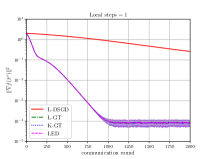
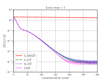
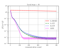
Figure 1: Simulation results for decentralized methods to achieve an approximate error of $10^{-4}$ under various local steps (L-DSGD [17, 11], LGT [42], and $K$-GT [43]). We emphasize that LED has half the communication cost of GT methods per communication round.

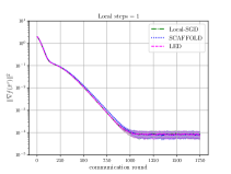
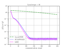
Figure 2: Simulation results for centralized methods to achieve an approximate error of $10^{-4}$ under various local steps (SCAFFOLD [10]). We emphasize that LED has half the communication cost of SCAFFOLD per communication round.

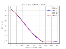
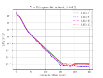
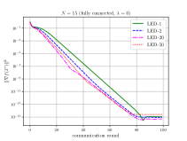
(a) Large data heterogeneity

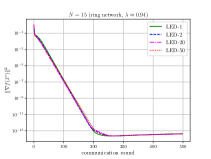
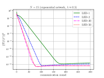
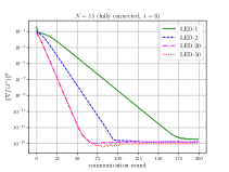
(b) Small data heterogeneity (similar data across the network)

Figure 3: LED simulation results in the deterministic case (zero noise $\sigma=0$). In this Figure, LED-$\uptau$ refers to LED with $\uptau$ local updates.

6 Concluding remarks

In this work, we proposed Local Exact-Diffusion (LED), a locally updated method inspired by the framework from [6] and the Exact-Diffusion method [12]. We demonstrated that LED can be interpreted as the primal-dual method PDFP2O/PAPC from [45, 46]. We also explored its connection with the following methods: Exact-Diffusion (ED) [12], NIDS [33], D² [34], Scaffnew [44], VRL-SGD [23], and FedGate [24]. We proved the convergence of LED in both convex and nonconvex settings and established bounds that offer improvements over existing decentralized methods. Finally, we provided numerical simulations to illustrate the effectiveness of the proposed algorithm.

A promising direction for future research involves examining LED in the context of probabilistic local updates. It’s worth exploring if the current analysis can be integrated with techniques from Scaffnew/ProxSkip [44] to understand the advantages of local steps in non-strongly-convex scenarios. Another potential avenue is broadening LED to accommodate time-varying stochastic graphs. Furthermore, it would be insightful to see if decentralized local methods might also offer advantages for other network coupling constraints, as seen in multitask problems or the distributed feature problem.

Appendix A Preliminary transformation

In this section, we will convert LED updates (6) into another form more suitable for our analysis. To that end, we will first introduce some notation that complements the notation (5).

A.1 Notation

The following quantities will be used in the analysis:

$$\bar{{\mathbf{x}}}^{r} \triangleq\mathbf{1}_{N}\otimes\bar{x}^{r},\quad\bar{x}^{r}\triangleq\frac{1}{N}\sum\limits_{i=1}^{N}x_{i}^{r},$$ (30a)

$$\overline{{\nabla}f}({\mathbf{x}}^{r}) \triangleq\frac{1}{N}\sum\limits_{i=1}^{N}{\nabla}f_{i}(x_{i}^{r})$$ (30b)

$${\mathbf{s}}_{t}^{r} \triangleq\nabla{\mathbf{F}}(\bm{\Phi}^{r}_{t};\bm{\xi}_{t})-\nabla{\mathbf{f}}(\bm{\Phi}^{r}_{t})$$ (30c)

$$\bar{s}_{t}^{r} \triangleq\frac{1}{N}\sum\limits_{i=1}^{N}\left(\nabla F_{i}(\phi^{r}_{i,t};\xi_{i,t})-\nabla f_{i}(\phi^{r}_{i,t})\right),$$ (30d)

$${\mathbf{z}}^{r} \triangleq{\mathbf{y}}^{r}+\frac{\alpha}{\beta}{\nabla}{\mathbf{f}}(\bar{{\mathbf{x}}}^{r}),$$ (30e)

$$\bar{{\mathbf{z}}}^{r} \triangleq\mathbf{1}_{N}\otimes\bar{z}^{r},\quad\bar{z}^{r}\triangleq\frac{1}{N}\sum\limits_{i=1}^{N}z_{i}^{r}.$$ (30f)

A.2 Weight matrix decomposition

We will use the structure of the weight matrix $W$ in our analysis, which is a requirement for our proof. As a result, we will now go over some facts about the matrix $W$. When Assumption 1 holds, then the weight matrix $W$ can be decomposed as follows [49, 27]:

$$W=\begin{bmatrix}\frac{1}{\sqrt{N}}\mathbf{1}&\widehat{Q}\end{bmatrix}\begin{bmatrix}1&0\\ 0&\widehat{\Lambda}\end{bmatrix}\begin{bmatrix}\frac{1}{\sqrt{N}}\mathbf{1}^{\textit{\footnotesize{T}}}\vspace{0.6mm}\\ \widehat{Q}^{\textit{\footnotesize{T}}}\end{bmatrix},$$

where $\widehat{\Lambda}={\rm diag}\{\lambda_{i}\}_{i=2}^{N}$ and the matrix $\widehat{Q}$ has size ${N\times(N-1)}$, and satisfies $\widehat{Q}\widehat{Q}^{\textit{\footnotesize{T}}}=I_{N}-\tfrac{1}{N}\mathbf{1}\mathbf{1}^{\textit{\footnotesize{T}}}$ and $\mathbf{1}^{\textit{\footnotesize{T}}}\widehat{Q}=0$. It follows that ${\mathbf{W}}\triangleq W\otimes I_{m}$ can be decomposed as

$${\mathbf{W}} =\begin{bmatrix}\frac{1}{\sqrt{N}}\mathbf{1}\otimes I_{m}&\widehat{{\mathbf{Q}}}\end{bmatrix}\begin{bmatrix}I_{m}&0\\ 0&\widehat{\mathbf{\Lambda}}\end{bmatrix}\begin{bmatrix}\frac{1}{\sqrt{N}}\mathbf{1}^{\textit{\footnotesize{T}}}\otimes I_{m}\\ \widehat{{\mathbf{Q}}}^{\textit{\footnotesize{T}}}\end{bmatrix}=\tfrac{1}{N}\mathbf{1}\mathbf{1}^{\textit{\footnotesize{T}}}\otimes I_{m}+\widehat{{\mathbf{Q}}}\widehat{\mathbf{\Lambda}}\widehat{{\mathbf{Q}}}^{\textit{\footnotesize{T}}},$$ (31a)

where $$\widehat{\mathbf{\Lambda}}\triangleq\widehat{\Lambda}\otimes I_{m}\in{}^{m(N-1)\times m(N-1)} \widehat{{\mathbf{Q}}}\triangleq\widehat{Q}\otimes I_{m}\in{}^{mN\times m(N-1)}$$ and satisfies:

$$\widehat{{\mathbf{Q}}}^{\textit{\footnotesize{T}}}\widehat{{\mathbf{Q}}}={\mathbf{I}},\quad\widehat{{\mathbf{Q}}}\widehat{{\mathbf{Q}}}^{\textit{\footnotesize{T}}}={\mathbf{I}}-\tfrac{1}{N}\mathbf{1}\mathbf{1}^{\textit{\footnotesize{T}}}\otimes I_{m},\quad(\mathbf{1}^{\textit{\footnotesize{T}}}\otimes I_{m})\widehat{{\mathbf{Q}}}=0.$$ (31b)

Below, we provide a list of relevant facts and properties concerning the aforementioned decomposition.

• It holds that

  $$\|\widehat{{\mathbf{Q}}}^{\textit{\footnotesize{T}}}{\mathbf{x}}^{r}\|^{2}=\|\widehat{{\mathbf{Q}}}\widehat{{\mathbf{Q}}}^{\textit{\footnotesize{T}}}{\mathbf{x}}^{r}\|^{2}=\|{\mathbf{x}}^{r}-\bar{{\mathbf{x}}}^{r}\|^{2},\quad\text{and}\quad\|\widehat{{\mathbf{Q}}}\|=1.$$ (32)

• The matrix $\widehat{{\mathbf{B}}}\triangleq{\mathbf{I}}-\widehat{\mathbf{\Lambda}}$ satisfies

  $$\|\widehat{{\mathbf{B}}}\|=1-\underline{\lambda}\leq 1\quad\text{and}\quad\|\widehat{{\mathbf{B}}}^{-1}\|=\frac{1}{1-\lambda},$$ (33)

  where $\underline{\lambda}$ is the smallest nonzero eigenvalue of $W$ and $\lambda$ is the network’s mixing rate introduced in (19).

A.3 Transformed recursion

To obtain our result, we will perform a series of transformations that will eventually lead us to the critical result specified in Lemma 1. In order to study the communication complexity of LED, we begin by representing it in terms of communication rounds. It holds true when iterating through (6a) updates:

$$\bm{\Phi}^{r}_{\uptau} ={\mathbf{x}}^{r}-\alpha\sum_{t=0}^{\uptau-1}\nabla{\mathbf{F}}(\bm{\Phi}^{r}_{t};\bm{\xi}_{t})-\beta\uptau{\mathbf{y}}^{r},$$

where $\bm{\Phi}^{r}_{0}={\mathbf{x}}^{r}$ and, for notational simplicity, we are removing the superscript in $\bm{\xi}_{t}^{r}$. Substituting the preceding into (6b) yields

$${\mathbf{x}}^{r+1} ={\mathbf{W}}\left({\mathbf{x}}^{r}-\beta\uptau{\mathbf{y}}^{r}-\alpha\sum_{t=0}^{\uptau-1}\nabla{\mathbf{F}}(\bm{\Phi}^{r}_{t};\bm{\xi}_{t})\right)$$ (34a)

$${\mathbf{y}}^{r+1} ={\mathbf{y}}^{r}+({\mathbf{I}}-{\mathbf{W}})\left({\mathbf{x}}^{r}-\beta\uptau{\mathbf{y}}^{r}-\alpha\sum_{t=0}^{\uptau-1}\nabla{\mathbf{F}}(\bm{\Phi}^{r}_{t};\bm{\xi}_{t})\right).$$ (34b)

Observe that under our initialization, ${\mathbf{y}}^{0}=({\mathbf{I}}-{\mathbf{W}}){\mathbf{x}}^{0}$, ${\mathbf{y}}^{r}$ will always be in the range of ${\mathbf{I}}-{\mathbf{W}}$. As a result, we have $(\mathbf{1}^{\textit{\footnotesize{T}}}\otimes I_{m}){\mathbf{y}}^{r}=0$ for all $r$. Multiplying both sides of (34a) by $(1/N)(\mathbf{1}^{\textit{\footnotesize{T}}}\otimes I_{m})$ on the left and using the definitions in (30) , namely $\overline{{\nabla}f}({\mathbf{x}}^{r})=\frac{1}{N}\sum_{i=1}^{N}{\nabla}f_{i}(x_{i}^{r}),\bar{s}_{t}^{r}=\frac{1}{N}\sum_{i=1}^{N}(\nabla F_{i}(\phi^{r}_{i,t};\xi_{i,t})-\nabla f_{i}(\phi^{r}_{i,t}))$], we get

$$\bar{x}^{r+1} =\bar{x}^{r}-\alpha\sum_{t=0}^{\uptau-1}\big{(}\overline{\nabla f}(\bm{\Phi}^{r}_{t})+\bar{s}_{t}^{r}\big{)}.$$ (35)

Equation (35) above describes how the average (centroid) vector evolves in terms of communication rounds, which will be important in our analysis. Now, using the definitions in (30), namely ${\mathbf{z}}^{r}={\mathbf{y}}^{r}+\frac{\alpha}{\beta}{\nabla}{\mathbf{f}}(\bar{{\mathbf{x}}}^{r})$ and ${\mathbf{s}}_{t}^{r}=\nabla{\mathbf{F}}(\bm{\Phi}^{r}_{t};\bm{\xi}_{t})-\nabla{\mathbf{f}}(\bm{\Phi}^{r}_{t})$, the update (34) can be equivalently described as

$${\mathbf{x}}^{r+1} ={\mathbf{W}}\left({\mathbf{x}}^{r}-\beta\uptau{\mathbf{z}}^{r}-\alpha\sum_{t=0}^{\uptau-1}\big{(}\nabla{\mathbf{f}}(\bm{\Phi}^{r}_{t})-{\nabla}{\mathbf{f}}(\bar{{\mathbf{x}}}^{r})+{\mathbf{s}}_{t}^{r}\big{)}\right)$$ (36a)

$${\mathbf{z}}^{r+1} =[(1-\beta\uptau){\mathbf{I}}+\beta\uptau{\mathbf{W}}]{\mathbf{z}}^{r}+({\mathbf{I}}-{\mathbf{W}}){\mathbf{x}}^{r}-\alpha({\mathbf{I}}-{\mathbf{W}})\sum_{t=0}^{\uptau-1}\big{(}\nabla{\mathbf{f}}(\bm{\Phi}^{r}_{t})-{\nabla}{\mathbf{f}}(\bar{{\mathbf{x}}}^{r})+{\mathbf{s}}_{t}^{r}\big{)}$$

$$\quad+\frac{\alpha}{\beta}\big{(}{\nabla}{\mathbf{f}}(\bar{{\mathbf{x}}}^{r+1})-{\nabla}{\mathbf{f}}(\bar{{\mathbf{x}}}^{r})\big{)}.$$ (36b)

Remark 7 (Deviation from Average).

The introduction of ${\mathbf{z}}^{r}$ is inspired from [29]. The quantity ${\mathbf{z}}^{r}$ can be interpreted as a variable that tracks the average gradient vector $\mathbf{1}\otimes{\nabla}f(\bar{x}^{r})$. Observe that by $(\mathbf{1}^{\textit{\footnotesize{T}}}\otimes I_{m}){\mathbf{y}}^{r}=0$ and (30e), we have

$$\bar{z}^{r}=(1/N)(\mathbf{1}^{\textit{\footnotesize{T}}}\otimes I_{m}){\mathbf{z}}^{r}=\frac{\alpha}{\beta N}\sum_{i=1}^{N}{\nabla}f_{i}(\bar{x}^{r}).$$ (37)

We will next transform the updates (36) into quantities that measure how far ${\mathbf{x}}^{r}$ and ${\mathbf{z}}^{r}$ deviate from the averages $\bar{{\mathbf{x}}}^{r}=\mathbf{1}_{N}\otimes\bar{x}^{r}$ and $\bar{{\mathbf{z}}}^{r}\triangleq\mathbf{1}_{N}\otimes\bar{z}^{r}$, respectively. To do so, we will leverage the structure and properties of the weight matrix ${\mathbf{W}}$ (32). $\blacksquare$

Using the decomposition of ${\mathbf{W}}$ given in (31), it holds that $\widehat{{\mathbf{Q}}}^{\textit{\footnotesize{T}}}{\mathbf{W}}=\widehat{\mathbf{\Lambda}}\widehat{{\mathbf{Q}}}^{\textit{\footnotesize{T}}}$. Therefore, multiplying both sides of (36) by $\widehat{{\mathbf{Q}}}^{\textit{\footnotesize{T}}}$, it holds that

$$\widehat{{\mathbf{Q}}}^{\textit{\footnotesize{T}}}{\mathbf{x}}^{r+1} =\widehat{\mathbf{\Lambda}}\widehat{{\mathbf{Q}}}^{\textit{\footnotesize{T}}}{\mathbf{x}}^{r}-\beta\uptau\widehat{\mathbf{\Lambda}}\widehat{{\mathbf{Q}}}^{\textit{\footnotesize{T}}}{\mathbf{z}}^{r}-\alpha\widehat{\mathbf{\Lambda}}\widehat{{\mathbf{Q}}}^{\textit{\footnotesize{T}}}\sum_{t=0}^{\uptau-1}\big{(}\nabla{\mathbf{f}}(\bm{\Phi}^{r}_{t})-{\nabla}{\mathbf{f}}(\bar{{\mathbf{x}}}^{r})+{\mathbf{s}}_{t}^{r}\big{)}$$ (38a)

$$\widehat{{\mathbf{Q}}}^{\textit{\footnotesize{T}}}{\mathbf{z}}^{r+1} =[(1-\beta\uptau){\mathbf{I}}+\beta\uptau\widehat{\mathbf{\Lambda}}]\widehat{{\mathbf{Q}}}^{\textit{\footnotesize{T}}}{\mathbf{z}}^{r}+({\mathbf{I}}-\widehat{\mathbf{\Lambda}})\widehat{{\mathbf{Q}}}^{\textit{\footnotesize{T}}}{\mathbf{x}}^{r}$$

$$\quad-\alpha({\mathbf{I}}-\widehat{\mathbf{\Lambda}})\widehat{{\mathbf{Q}}}^{\textit{\footnotesize{T}}}\sum_{t=0}^{\uptau-1}\big{(}\nabla{\mathbf{f}}(\bm{\Phi}^{r}_{t})-{\nabla}{\mathbf{f}}(\bar{{\mathbf{x}}}^{r})+{\mathbf{s}}_{t}^{r}\big{)}+\frac{\alpha}{\beta}\widehat{{\mathbf{Q}}}^{\textit{\footnotesize{T}}}\big{(}{\nabla}{\mathbf{f}}(\bar{{\mathbf{x}}}^{r+1})-{\nabla}{\mathbf{f}}(\bar{{\mathbf{x}}}^{r})\big{)}.$$ (38b)

Rewriting (38) in matrix notation, we have

$$\begin{bmatrix}\widehat{{\mathbf{Q}}}^{\textit{\footnotesize{T}}}{\mathbf{x}}^{r+1}\\ \widehat{{\mathbf{Q}}}^{\textit{\footnotesize{T}}}{\mathbf{z}}^{r+1}\end{bmatrix} =\begin{bmatrix}\widehat{\mathbf{\Lambda}}&-\beta\uptau\widehat{\mathbf{\Lambda}}\\ {\mathbf{I}}-\widehat{\mathbf{\Lambda}}&(1-\beta\uptau){\mathbf{I}}+\beta\uptau\widehat{\mathbf{\Lambda}}\end{bmatrix}\begin{bmatrix}\widehat{{\mathbf{Q}}}^{\textit{\footnotesize{T}}}{\mathbf{x}}^{r}\\ \widehat{{\mathbf{Q}}}^{\textit{\footnotesize{T}}}{\mathbf{z}}^{r}\end{bmatrix}$$

$$\quad-\alpha\begin{bmatrix}\widehat{\mathbf{\Lambda}}\widehat{{\mathbf{Q}}}^{\textit{\footnotesize{T}}}\sum\limits_{t=0}^{\uptau-1}\big{(}\nabla{\mathbf{f}}(\bm{\Phi}^{r}_{t})-{\nabla}{\mathbf{f}}(\bar{{\mathbf{x}}}^{r})+{\mathbf{s}}_{t}^{r}\big{)}\\ ({\mathbf{I}}-\widehat{\mathbf{\Lambda}})\widehat{{\mathbf{Q}}}^{\textit{\footnotesize{T}}}\sum\limits_{t=0}^{\uptau-1}\big{(}\nabla{\mathbf{f}}(\bm{\Phi}^{r}_{t})-{\nabla}{\mathbf{f}}(\bar{{\mathbf{x}}}^{r})+{\mathbf{s}}_{t}^{r}\big{)}-\frac{1}{\beta}\widehat{{\mathbf{Q}}}^{\textit{\footnotesize{T}}}\big{(}{\nabla}{\mathbf{f}}(\bar{{\mathbf{x}}}^{r+1})-{\nabla}{\mathbf{f}}(\bar{{\mathbf{x}}}^{r})\big{)}\end{bmatrix}.$$ (39)

Note that from (32), we have $\|\widehat{{\mathbf{Q}}}^{\textit{\footnotesize{T}}}{\mathbf{x}}^{r}\|^{2}=\|{\mathbf{x}}^{r}-\bar{{\mathbf{x}}}^{r}\|^{2}$ and similarly $\|\widehat{{\mathbf{Q}}}^{\textit{\footnotesize{T}}}{\mathbf{z}}^{r}\|^{2}=\|{\mathbf{z}}^{r}-\bar{{\mathbf{z}}}^{r}\|^{2}$. Thus, the above describes how the nodes vectors deviates from the averages. For $\beta=1/\uptau$, we will let

$${\mathbf{D}}\triangleq\begin{bmatrix}\widehat{\mathbf{\Lambda}}&-\beta\uptau\widehat{\mathbf{\Lambda}}\\ {\mathbf{I}}-\widehat{\mathbf{\Lambda}}&(1-\beta\uptau){\mathbf{I}}+\beta\uptau\widehat{\mathbf{\Lambda}}\end{bmatrix} =\begin{bmatrix}\widehat{\mathbf{\Lambda}}&-\widehat{\mathbf{\Lambda}}\\ {\mathbf{I}}-\widehat{\mathbf{\Lambda}}&~{}~{}\widehat{\mathbf{\Lambda}}\end{bmatrix}=\begin{bmatrix}\widehat{\Lambda}&-\widehat{\Lambda}\\ I-\widehat{\Lambda}&~{}~{}\widehat{\Lambda}\end{bmatrix}\otimes I_{m}.$$ (40)

If the norm of the matrix ${\mathbf{D}}$ is less than one $\|{\mathbf{D}}\|<1$, then the updates (A.3) can be used to directly measure the deviation from the averages. However, even though the eigenvalues of ${\mathbf{D}}$ are less than one, its norm is not guaranteed to satisfy $\|{\mathbf{D}}\|<1$; but, we can decompose ${\mathbf{D}}$ and transform (A.3) into a more suitable form for our analysis, as shown in the important result below.

Lemma 1 (Deviation from average).

Suppose that Assumption 1 holds and $\beta=1/\uptau$, then

$$\widehat{{\mathbf{d}}}^{r+1} =\mathbf{\Delta}\widehat{{\mathbf{d}}}^{r}-\alpha\widehat{{\mathbf{V}}}^{-1}\begin{bmatrix}\widehat{\mathbf{\Lambda}}\widehat{{\mathbf{Q}}}^{\textit{\footnotesize{T}}}\sum\limits_{t=0}^{\uptau-1}\big{(}\nabla{\mathbf{f}}(\bm{\Phi}^{r}_{t})-{\nabla}{\mathbf{f}}(\bar{{\mathbf{x}}}^{r})+{\mathbf{s}}_{t}^{r}\big{)}\\ \widehat{{\mathbf{B}}}\widehat{{\mathbf{Q}}}^{\textit{\footnotesize{T}}}\sum\limits_{t=0}^{\uptau-1}\big{(}\nabla{\mathbf{f}}(\bm{\Phi}^{r}_{t})-{\nabla}{\mathbf{f}}(\bar{{\mathbf{x}}}^{r})+{\mathbf{s}}_{t}^{r}\big{)}-\uptau\widehat{{\mathbf{Q}}}^{\textit{\footnotesize{T}}}\big{(}{\nabla}{\mathbf{f}}(\bar{{\mathbf{x}}}^{r+1})-{\nabla}{\mathbf{f}}(\bar{{\mathbf{x}}}^{r})\big{)}\end{bmatrix},$$ (41)

where $\mathbf{\Delta}$ is a matrix with norm $\delta\triangleq\|\mathbf{\Delta}\|=\sqrt{\lambda}<1$, $\widehat{{\mathbf{B}}}\triangleq{\mathbf{I}}-\widehat{\mathbf{\Lambda}}$, and

$$\widehat{{\mathbf{d}}}^{r} \triangleq\widehat{{\mathbf{V}}}^{-1}\begin{bmatrix}\widehat{{\mathbf{Q}}}^{\textit{\footnotesize{T}}}{\mathbf{x}}^{r}\\ \widehat{{\mathbf{Q}}}^{\textit{\footnotesize{T}}}{\mathbf{z}}^{r}\end{bmatrix}$$ (42a)

$$\widehat{{\mathbf{V}}}^{-1} \triangleq{\mathbf{P}}\begin{bmatrix}\frac{1}{2}\widehat{\mathbf{\Lambda}}^{-\frac{1}{2}}&\frac{\jmath}{2}\widehat{{\mathbf{B}}}^{-\frac{1}{2}}\\ \frac{1}{2}\widehat{\mathbf{\Lambda}}^{-\frac{1}{2}}&-\frac{\jmath}{2}\widehat{{\mathbf{B}}}^{-\frac{1}{2}}\end{bmatrix},\quad\widehat{{\mathbf{V}}}\triangleq\begin{bmatrix}\widehat{\mathbf{\Lambda}}^{\frac{1}{2}}&\widehat{\mathbf{\Lambda}}^{\frac{1}{2}}\\ -\jmath\widehat{{\mathbf{B}}}^{\frac{1}{2}}&\jmath\widehat{{\mathbf{B}}}^{\frac{1}{2}}\end{bmatrix}{\mathbf{P}}^{\textit{\footnotesize{T}}}.$$ (42b)

Here, ${\mathbf{P}}$ is some permutation matrix and $\jmath=\sqrt{-1}$ is the imaginary number.

Proof.

The proof exploits the special structure of the matrix ${\mathbf{D}}$ given in (40). First note that if

$$A=\begin{bmatrix}{\rm diag}\{b_{i}\}_{i=2}^{N}&{\rm diag}\{c_{i}\}_{i=2}^{N}\\ {\rm diag}\{d_{i}\}_{i=2}^{N}&{\rm diag}\{e_{i}\}_{i=2}^{N}\end{bmatrix}\triangleq\begin{bmatrix}B&C\\ D&E\end{bmatrix}.$$ (43)

where $b_{i},c_{i},d_{i},e_{i}$ are constants, then there exists a permutation matrix $P$ such that

$$PAP^{\textit{\footnotesize{T}}}={\rm blkdiag}\{A_{i}\}_{i=2}^{N},\quad A_{i}=\begin{bmatrix}b_{i}&c_{i}\\ d_{i}&e_{i}\end{bmatrix}.$$ (44)

Since the blocks of ${\mathbf{D}}$ given in (40) are diagonal matrices, there exists a permutation matrix ${\mathbf{P}}$ such that

$${\mathbf{P}}{\mathbf{D}}{\mathbf{P}}^{\textit{\footnotesize{T}}}={\rm blkdiag}\{D_{i}\}_{i=2}^{N}\otimes I_{m},\quad D_{i}=\begin{bmatrix}\lambda_{i}&-\lambda_{i}\\ 1-\lambda_{i}&~{}~{}\lambda_{i}\end{bmatrix}\in{}^{2\times 2}.$$

The eigenvalues of $D_{i}$ ($i=2,\ldots,N$) are

$$\delta_{(1,2),i} =(1/2)\left[\mathop{\rm Tr}(D_{i})\pm\sqrt{\mathop{\rm Tr}(D_{i})^{2}-4\det(D_{i})}\right]$$

$$=\lambda_{i}\pm\sqrt{\lambda_{i}^{2}-\lambda_{i}}.$$

Notice that $|\delta_{(1,2),i}|<1$ when $-\frac{1}{3}<\lambda_{i}<1$, which holds under Assumption 1 since $W>0$, i.e., $0<\lambda_{i}<1$ ($i=2,\dots,N$). For $0<\lambda_{i}<1$, the eigenvalues of $D_{i}$ are complex and distinct:

$$\delta_{(1,2),i}=\lambda_{i}\pm\jmath\sqrt{\lambda_{i}-\lambda_{i}^{2}},\qquad|\delta_{(1,2),i}|=\sqrt{\lambda_{i}}<1,$$

where $\jmath^{2}=-1$. Through algebraic multiplication it can be verified that $D_{i}=V_{i}\Delta_{i}V_{i}^{-1}$ where

$$\Delta_{i}=\begin{bmatrix}\lambda_{i}+\jmath\sqrt{\lambda_{i}-\lambda_{i}^{2}}&0\\ 0&\lambda_{i}-\jmath\sqrt{\lambda_{i}-\lambda_{i}^{2}},\end{bmatrix}$$ (45)

and

$$V_{i}=\begin{bmatrix}\sqrt{\lambda_{i}}&\sqrt{\lambda_{i}}\\ -\jmath\sqrt{1-\lambda_{i}}&\jmath\sqrt{1-\lambda_{i}}\end{bmatrix},\quad V_{i}^{-1}=\begin{bmatrix}\frac{1}{2\sqrt{\lambda_{i}}}&\frac{\jmath}{2\sqrt{1-\lambda_{i}}}\\ \frac{1}{2\sqrt{\lambda_{i}}}&-\frac{\jmath}{2\sqrt{1-\lambda_{i}}}\end{bmatrix}.$$ (46)

We conclude that ${\mathbf{D}}={\mathbf{P}}^{\textit{\footnotesize{T}}}{\mathbf{V}}\mathbf{\Delta}{\mathbf{V}}^{-1}{\mathbf{P}}$ where ${\mathbf{V}}={\rm blkdiag}\{V_{i}\}_{i=2}^{N}\otimes I_{m}$ and $\mathbf{\Delta}={\rm blkdiag}\{\Delta_{i}\}_{i=2}^{N}\otimes I_{m}$. Therefore, left multiplying both sides of (A.3) by $\widehat{{\mathbf{V}}}^{-1}$ where $\widehat{{\mathbf{V}}}={\mathbf{P}}^{\textit{\footnotesize{T}}}{\mathbf{V}}$ gives (41). Exploiting the structure of ${\mathbf{V}}^{-1}={\rm blkdiag}\{V_{i}^{-1}\}_{i=2}^{N}\otimes I_{m}$ where $V_{i}^{-1}$ is defined in (46) and using (44), we get

$$\widehat{{\mathbf{V}}}^{-1}={\mathbf{V}}^{-1}{\mathbf{P}}={\mathbf{P}}({\mathbf{P}}^{\textit{\footnotesize{T}}}{\mathbf{V}}^{-1}{\mathbf{P}}) ={\mathbf{P}}\begin{bmatrix}{\rm diag}\{\frac{1}{2\sqrt{\lambda_{i}}}\}_{i=2}^{N}&{\rm diag}\{\frac{\jmath}{2\sqrt{1-\lambda_{i}}}\}_{i=2}^{N}\\ {\rm diag}\{\frac{1}{2\sqrt{\lambda_{i}}}\}_{i=2}^{N}&-{\rm diag}\{\frac{\jmath}{2\sqrt{1-\lambda_{i}}}\}_{i=2}^{N}\end{bmatrix}\otimes I_{m}$$

$$={\mathbf{P}}\begin{bmatrix}\frac{1}{2}\widehat{\mathbf{\Lambda}}^{-\frac{1}{2}}&\frac{\jmath}{2}({\mathbf{I}}-\widehat{\mathbf{\Lambda}})^{-\frac{1}{2}}\\ \frac{1}{2}\widehat{\mathbf{\Lambda}}^{-\frac{1}{2}}&-\frac{\jmath}{2}({\mathbf{I}}-\widehat{\mathbf{\Lambda}})^{-\frac{1}{2}}\end{bmatrix}.$$

Using similar arguments for ${\mathbf{V}}$ gives (42b).

∎

Remark 8 (Centralized case).

The transformation in Lemma 1 is needed for decentralized network analysis since, as explained before, the norm of the matrix ${\mathbf{D}}$ (40) is not necessarily less than one. However, when the network is fully-connected (centralized case), we have $\widehat{\mathbf{\Lambda}}=\mathbf{0}$, and thus, it follows from (A.3) that $\widehat{{\mathbf{Q}}}^{\textit{\footnotesize{T}}}{\mathbf{x}}^{r}=\mathbf{0}$ and when $\beta=1/\uptau$, we have

$${\mathbf{d}}^{r+1}_{\rm cen}\triangleq\widehat{{\mathbf{Q}}}^{\textit{\footnotesize{T}}}{\mathbf{z}}^{r+1} =-\alpha\widehat{{\mathbf{Q}}}^{\textit{\footnotesize{T}}}\sum_{t=0}^{\uptau-1}\big{(}\nabla{\mathbf{f}}(\bm{\Phi}^{r}_{t})-{\nabla}{\mathbf{f}}(\bar{{\mathbf{x}}}^{r})+{\mathbf{s}}_{t}^{r}\big{)}+\uptau\alpha\widehat{{\mathbf{Q}}}^{\textit{\footnotesize{T}}}\big{(}{\nabla}{\mathbf{f}}(\bar{{\mathbf{x}}}^{r+1})-{\nabla}{\mathbf{f}}(\bar{{\mathbf{x}}}^{r})\big{)}.$$ (47)

In this case, the analysis can be greatly simplified since ${\mathbf{D}}=\mathbf{0}$. This specialization covers the method VRL-SGD [23]. A similar approach can also be adapted to FedGate [24], as described in (18). Doing so eventually leads to the result in Corollary LABEL:cor_centralized. See Appendix D. $\blacksquare$

Appendix B Convergence analysis

In this section, we will prove Theorems 1 and 2. The proof utilizes equations (35) and (41) derived in the previous section. We want to emphasize that some of the bounds may appear tedious, even though they only involve basic algebra. Such complexity is common in decentralized analysis, as seen in, for example, [29, 50].

B.1 Auxiliary results

In the proof, we will use the following useful results and facts. (You may overlook and refer to this subsection later in the proofs.)

• Since the squared norm $\|\cdot\|^{2}$ is convex, applying Jensen’s inequality, it holds that [51]

  $$\|{\textstyle\sum\limits_{k=1}^{K}}a_{k}\|^{2}\leq K\sum_{k=1}^{K}\left\|a_{k}\right\|^{2},$$ (48a)

  for all vectors $$\{a_{k}\}_{k=1}^{K} K a b \theta\in(0,1)$$ of equal size and positive integer . Moreover, for any equal-size vectors and , we have for :

  $$\|a+b\|^{2}\leq\frac{1}{\theta}\|a\|^{2}+\frac{1}{1-\theta}\|b\|^{2}.$$ (48b)

  Many bounds later in the proofs uses inequality (48a) without referring to it to avoid redundancies.

• Taking the squared norm on both sides of (42a) and using (48a), it holds that:

  $$\|\widehat{{\mathbf{d}}}^{r}\|^{2}\leq\frac{1}{4}\left\|\begin{bmatrix}\widehat{\mathbf{\Lambda}}^{-\frac{1}{2}}\widehat{{\mathbf{Q}}}^{\textit{\footnotesize{T}}}{\mathbf{x}}^{r}+\jmath\widehat{{\mathbf{B}}}^{-\frac{1}{2}}\widehat{{\mathbf{Q}}}^{\textit{\footnotesize{T}}}{\mathbf{z}}^{r}\\ \widehat{\mathbf{\Lambda}}^{-\frac{1}{2}}\widehat{{\mathbf{Q}}}^{\textit{\footnotesize{T}}}{\mathbf{x}}^{r}-\widehat{{\mathbf{B}}}^{-\frac{1}{2}}\widehat{{\mathbf{Q}}}^{\textit{\footnotesize{T}}}{\mathbf{z}}^{r}\end{bmatrix}\right\|^{2}\leq\|\widehat{\mathbf{\Lambda}}^{-\frac{1}{2}}\widehat{{\mathbf{Q}}}^{\textit{\footnotesize{T}}}{\mathbf{x}}^{r}\|^{2}+\|\widehat{{\mathbf{B}}}^{-\frac{1}{2}}\widehat{{\mathbf{Q}}}^{\textit{\footnotesize{T}}}{\mathbf{z}}^{r}\|^{2}.$$ (49)

• From (42a)–(42b), it holds that

  $$\begin{bmatrix}\widehat{{\mathbf{Q}}}^{\textit{\footnotesize{T}}}{\mathbf{x}}^{r}\\ \widehat{{\mathbf{Q}}}^{\textit{\footnotesize{T}}}{\mathbf{z}}^{r}\end{bmatrix}=\begin{bmatrix}\widehat{\mathbf{\Lambda}}^{\frac{1}{2}}&\widehat{\mathbf{\Lambda}}^{\frac{1}{2}}\\ -\jmath\widehat{{\mathbf{B}}}^{\frac{1}{2}}&\jmath\widehat{{\mathbf{B}}}^{\frac{1}{2}}\end{bmatrix}{\mathbf{P}}^{\textit{\footnotesize{T}}}\widehat{{\mathbf{d}}}^{r}=\begin{bmatrix}\widehat{\mathbf{\Lambda}}^{\frac{1}{2}}({\mathbf{P}}_{u}^{\textit{\footnotesize{T}}}+{\mathbf{P}}_{l}^{\textit{\footnotesize{T}}})\widehat{{\mathbf{d}}}^{r}\\ -\jmath\widehat{{\mathbf{B}}}^{\frac{1}{2}}({\mathbf{P}}_{u}^{\textit{\footnotesize{T}}}-{\mathbf{P}}_{l}^{\textit{\footnotesize{T}}})\widehat{{\mathbf{d}}}^{r}\end{bmatrix},$$ (50)

  where ${\mathbf{P}}_{u}^{\textit{\footnotesize{T}}}$ and ${\mathbf{P}}_{l}^{\textit{\footnotesize{T}}}$ are the upper and lower blocks of ${\mathbf{P}}^{\textit{\footnotesize{T}}}=[{\mathbf{P}}_{u}^{\textit{\footnotesize{T}}};{\mathbf{P}}_{l}^{\textit{\footnotesize{T}}}]$. It follows that:

  $$\|{\mathbf{x}}^{r}-\bar{{\mathbf{x}}}^{r}\|^{2} =\|\widehat{{\mathbf{Q}}}^{\textit{\footnotesize{T}}}{\mathbf{x}}^{r}\|^{2}=\|\widehat{\mathbf{\Lambda}}^{\frac{1}{2}}({\mathbf{P}}_{u}^{\textit{\footnotesize{T}}}+{\mathbf{P}}_{l}^{\textit{\footnotesize{T}}})\widehat{{\mathbf{d}}}^{r}\|^{2}\leq 4\lambda\|\widehat{{\mathbf{d}}}^{r}\|^{2}$$ (51a)

  $$\|{\mathbf{z}}^{r}-\bar{{\mathbf{z}}}^{r}\|^{2} =\|\widehat{{\mathbf{Q}}}^{\textit{\footnotesize{T}}}{\mathbf{z}}^{r}\|^{2}=\|-\jmath\widehat{{\mathbf{B}}}^{\frac{1}{2}}({\mathbf{P}}_{u}^{\textit{\footnotesize{T}}}-{\mathbf{P}}_{l}^{\textit{\footnotesize{T}}})\widehat{{\mathbf{d}}}^{r}\|^{2}\leq 4\|\widehat{{\mathbf{B}}}\|\|\widehat{{\mathbf{d}}}^{r}\|^{2},$$ (51b)

  where we used $\|{\mathbf{P}}_{u}^{\textit{\footnotesize{T}}}+{\mathbf{P}}_{l}^{\textit{\footnotesize{T}}}\|^{2}\leq 4$ and $\|{\mathbf{P}}_{u}^{\textit{\footnotesize{T}}}-{\mathbf{P}}_{l}^{\textit{\footnotesize{T}}}\|^{2}\leq 4$ since ${\mathbf{P}}$ is a permutation matrix $\|{\mathbf{P}}\|=1$.

• It holds that

  $${\mathbf{s}}^{r}\triangleq\widehat{{\mathbf{V}}}^{-1}\begin{bmatrix}\widehat{\mathbf{\Lambda}}\widehat{{\mathbf{Q}}}^{\textit{\footnotesize{T}}}\sum\limits_{t=0}^{\uptau-1}{\mathbf{s}}_{t}^{r}\\ \widehat{{\mathbf{B}}}\widehat{{\mathbf{Q}}}^{\textit{\footnotesize{T}}}\sum\limits_{t=0}^{\uptau-1}{\mathbf{s}}_{t}^{r}\end{bmatrix} {=}{\mathbf{P}}\begin{bmatrix}\frac{1}{2}\widehat{\mathbf{\Lambda}}^{-\frac{1}{2}}&\frac{\jmath}{2}\widehat{{\mathbf{B}}}^{-\frac{1}{2}}\\ \frac{1}{2}\widehat{\mathbf{\Lambda}}^{-\frac{1}{2}}&-\frac{\jmath}{2}\widehat{{\mathbf{B}}}^{-\frac{1}{2}}\end{bmatrix}\begin{bmatrix}\widehat{\mathbf{\Lambda}}\widehat{{\mathbf{Q}}}^{\textit{\footnotesize{T}}}\sum\limits_{t=0}^{\uptau-1}{\mathbf{s}}_{t}^{r}\\ \widehat{{\mathbf{B}}}\widehat{{\mathbf{Q}}}^{\textit{\footnotesize{T}}}\sum\limits_{t=0}^{\uptau-1}{\mathbf{s}}_{t}^{r}\end{bmatrix}$$ (52)

  $$=\tfrac{1}{2}{\mathbf{P}}\begin{bmatrix}\widehat{\mathbf{\Lambda}}^{\frac{1}{2}}\widehat{{\mathbf{Q}}}^{\textit{\footnotesize{T}}}\sum\limits_{t=0}^{\uptau-1}{\mathbf{s}}_{t}^{r}+\jmath\widehat{{\mathbf{B}}}^{\frac{1}{2}}\widehat{{\mathbf{Q}}}^{\textit{\footnotesize{T}}}\sum\limits_{t=0}^{\uptau-1}{\mathbf{s}}_{t}^{r}\\ \widehat{\mathbf{\Lambda}}^{\frac{1}{2}}\widehat{{\mathbf{Q}}}^{\textit{\footnotesize{T}}}\sum\limits_{t=0}^{\uptau-1}{\mathbf{s}}_{t}^{r}-\jmath\widehat{{\mathbf{B}}}^{\frac{1}{2}}\widehat{{\mathbf{Q}}}^{\textit{\footnotesize{T}}}\sum\limits_{t=0}^{\uptau-1}{\mathbf{s}}_{t}^{r}\end{bmatrix}.$$ (53)

  Therefore,

  $$\|{\mathbf{s}}^{r}\|^{2} \leq\tfrac{1}{4}\left(\|\widehat{\mathbf{\Lambda}}^{\frac{1}{2}}\widehat{{\mathbf{Q}}}^{\textit{\footnotesize{T}}}\textstyle\sum\limits_{t=0}^{\uptau-1}{\mathbf{s}}_{t}^{r}+\jmath\widehat{{\mathbf{B}}}^{\frac{1}{2}}\widehat{{\mathbf{Q}}}^{\textit{\footnotesize{T}}}\sum\limits_{t=0}^{\uptau-1}{\mathbf{s}}_{t}^{r}\|^{2}+\|\widehat{\mathbf{\Lambda}}^{\frac{1}{2}}\widehat{{\mathbf{Q}}}^{\textit{\footnotesize{T}}}\sum\limits_{t=0}^{\uptau-1}{\mathbf{s}}_{t}^{r}-\jmath\widehat{{\mathbf{B}}}^{\frac{1}{2}}\widehat{{\mathbf{Q}}}^{\textit{\footnotesize{T}}}\sum\limits_{t=0}^{\uptau-1}{\mathbf{s}}_{t}^{r}\|^{2}\right)$$

  $$\leq 2\|\textstyle\sum\limits_{t=0}^{\uptau-1}{\mathbf{s}}_{t}^{r}\|^{2}.$$ (54)

  The last step holds by using Jensen’s inequality (48) and (32)–(33). Following similar arguments, it can be shown that the squared norm of

  $${\mathbf{h}}^{r+1} \triangleq\widehat{{\mathbf{V}}}^{-1}\begin{bmatrix}\widehat{\mathbf{\Lambda}}\widehat{{\mathbf{Q}}}^{\textit{\footnotesize{T}}}\sum\limits_{t}\big{(}\nabla{\mathbf{f}}(\bm{\Phi}^{r}_{t})-{\nabla}{\mathbf{f}}(\bar{{\mathbf{x}}}^{r})\big{)}\\ \widehat{{\mathbf{B}}}\widehat{{\mathbf{Q}}}^{\textit{\footnotesize{T}}}\sum\limits_{t}\big{(}\nabla{\mathbf{f}}(\bm{\Phi}^{r}_{t})-{\nabla}{\mathbf{f}}(\bar{{\mathbf{x}}}^{r})\big{)}-\uptau\widehat{{\mathbf{Q}}}^{\textit{\footnotesize{T}}}\big{(}{\nabla}{\mathbf{f}}(\bar{{\mathbf{x}}}^{r+1})-{\nabla}{\mathbf{f}}(\bar{{\mathbf{x}}}^{r})\big{)}\end{bmatrix}.$$ (55)

  is upper bounded by

  $$\|{\mathbf{h}}^{r+1}\|^{2} \leq 4\|\textstyle\sum\limits_{t=0}^{\uptau-1}\nabla{\mathbf{f}}(\bm{\Phi}^{r}_{t})-{\nabla}{\mathbf{f}}(\bar{{\mathbf{x}}}^{r})\|^{2}+\uptau^{2}\|\widehat{{\mathbf{B}}}^{-1}\|\|{\nabla}{\mathbf{f}}(\bar{{\mathbf{x}}}^{r+1})-{\nabla}{\mathbf{f}}(\bar{{\mathbf{x}}}^{r})\|^{2}.$$ (56)

B.2 Key bounds

In this section, we derive some key bounds that will be used to establish our result for both nonconvex and convex cases.

The first bound involves the cumulative deviation of the local updates from the averaged vector at the previous communication round defined as

$$\|\bm{\widehat{\Phi}}^{r}\|^{2}\triangleq\sum\limits_{t=0}^{\uptau-1}\|\bm{\Phi}^{r}_{t}-\bar{{\mathbf{x}}}^{r}\|^{2}=\sum_{t=0}^{\uptau-1}\sum_{i=1}^{N}\|\phi^{r}_{i,t}-\bar{x}^{r}\|^{2}.$$ (57)

where $\bm{\widehat{\Phi}}^{r}\triangleq\mathrm{col}\{\bm{\Phi}^{r}_{t}-\bar{{\mathbf{x}}}^{r}\}_{t=0}^{\uptau-1}$. The term (57) will appear frequently in our analysis.

Lemma 2 (Local steps bound).

Let Assumptions 2–3 hold, then for $\alpha\leq\frac{1}{2\sqrt{2}L\uptau}$ we have

$$\mathop{\mathbb{E}{}}\|\bm{\widehat{\Phi}}^{r}\|^{2} \leq 64\uptau\mathop{\mathbb{E}{}}\|\widehat{{\mathbf{d}}}^{r}\|^{2}+16\alpha^{2}\uptau^{3}N\mathop{\mathbb{E}{}}\|{\nabla}f(\bar{x}^{r})\|^{2}+4\alpha^{2}\uptau^{2}N\sigma^{2}.$$ (58)

Proof.

The proof extends the techniques from [10, Lemma 8]. When $\uptau=1$, then $\phi_{i,0}=x_{i}^{r}$ for all $i$ and

$$\mathop{\mathbb{E}{}}\|\bm{\widehat{\Phi}}^{r}\|^{2}=\mathop{\mathbb{E}{}}\|{\mathbf{x}}^{r}-\bar{{\mathbf{x}}}^{r}\|^{2}\overset{\eqref{dhat_bound_x_z_dev}}{\leq}4\lambda\mathop{\mathbb{E}{}}\|\widehat{{\mathbf{d}}}^{r}\|^{2}\leq 4\mathop{\mathbb{E}{}}\|\widehat{{\mathbf{d}}}^{r}\|^{2}.$$

Now suppose that $\uptau\geq 2$. Then, using (6a), it holds that

$$\mathop{\mathbb{E}{}}\|\phi^{r}_{i,t+1}-\bar{x}^{r}\|^{2} =\mathop{\mathbb{E}{}}\left\|\phi^{r}_{i,t}-\bar{x}^{r}-\alpha{\nabla}F_{i}(\phi^{r}_{i,t};\xi_{i,t})-\beta y_{i}^{r}\right\|^{2}$$

$$\overset{\eqref{noise_bound_eq}}{} {\leq}\mathop{\mathbb{E}{}}\left\|\phi^{r}_{i,t}-\bar{x}^{r}-\alpha{\nabla}f_{i}(\phi^{r}_{i,t})-\beta y_{i}^{r}\right\|^{2}+\alpha^{2}\sigma^{2}$$

$$\overset{\eqref{jensens_b}}{} {\leq}\left(1+\tfrac{1}{\uptau-1}\right)\mathop{\mathbb{E}{}}\left\|\phi^{r}_{i,t}-\bar{x}^{r}\right\|^{2}+\uptau\mathop{\mathbb{E}{}}\left\|\alpha{\nabla}f_{i}(\phi^{r}_{i,t})+\beta y_{i}^{r}\right\|^{2}+\alpha^{2}\sigma^{2}$$

$$\overset{\eqref{z_def}}{} {=}\left(1+\tfrac{1}{\uptau-1}\right)\mathop{\mathbb{E}{}}\|\phi^{r}_{i,t}-\bar{x}^{r}\|^{2}+\uptau\mathop{\mathbb{E}{}}\left\|\alpha{\nabla}f_{i}(\phi^{r}_{i,t})-\alpha{\nabla}f_{i}(\bar{x}^{r})+\beta z_{i}^{r}\right\|^{2}+\alpha^{2}\sigma^{2}$$

$$\overset{\eqref{jensens_a}}{} {\leq}\left(1+\tfrac{1}{\uptau-1}\right)\mathop{\mathbb{E}{}}\|\phi^{r}_{i,t}-\bar{x}^{r}\|^{2}+2\alpha^{2}\uptau\mathop{\mathbb{E}{}}\left\|{\nabla}f_{i}(\phi^{r}_{i,t})-{\nabla}f_{i}(\bar{x}^{r})\right\|^{2}+2\uptau\beta^{2}\|z_{i}^{r}\|^{2}+\alpha^{2}\sigma^{2}$$

$$\overset{\eqref{smooth_f_eq}}{} {\leq}\left(1+\tfrac{1}{\uptau-1}+2\alpha^{2}\uptau L^{2}\right)\mathop{\mathbb{E}{}}\|\phi^{r}_{i,t}-\bar{x}^{r}\|^{2}+\tfrac{2}{\uptau}\mathop{\mathbb{E}{}}\left\|z_{i}^{r}\right\|^{2}+\alpha^{2}\sigma^{2}$$

$$\leq\left(1+\tfrac{5/4}{\uptau-1}\right)\mathop{\mathbb{E}{}}\|\phi^{r}_{i,t}-\bar{x}^{r}\|^{2}+\tfrac{2}{\uptau}\mathop{\mathbb{E}{}}\|z_{i}^{r}\|^{2}+\alpha^{2}\sigma^{2}.$$

The second inequality uses (48b) with $\theta=1-\frac{1}{\uptau}$. The last inequality holds for $2\alpha^{2}\uptau L^{2}\leq\frac{1}{4(\uptau-1)}$, which is satisfied if $\alpha\leq\frac{1}{2\sqrt{2}L\uptau}$. Iterating the inequality above for $t=0,\dots,\uptau-1$:

$$\mathop{\mathbb{E}{}}\|\phi^{r}_{i,t+1}-\bar{x}^{r}\|^{2} \leq\left(1+\tfrac{5/4}{(\uptau-1)}\right)^{t}\mathop{\mathbb{E}{}}\|x_{i}^{r}-\bar{x}^{r}\|^{2}+\textstyle\sum\limits_{\ell=0}^{t}\left(\tfrac{2}{\uptau}\mathop{\mathbb{E}{}}\left\|z_{i}^{r}\right\|^{2}+\alpha^{2}\sigma^{2}\right)\left(1+\frac{5/4}{(\uptau-1)}\right)^{\ell}$$

$$\leq\exp\left(\tfrac{(5/4)t}{\uptau-1}\right)\mathop{\mathbb{E}{}}\|x_{i}^{r}-\bar{x}^{r}\|^{2}+\textstyle\sum\limits_{\ell=0}^{t}\left(\tfrac{2}{\uptau}\mathop{\mathbb{E}{}}\left\|z_{i}^{r}\right\|^{2}+\alpha^{2}\sigma^{2}\right)\exp\left(\tfrac{(5/4)\ell}{\uptau-1}\right)$$

$$\leq 4\mathop{\mathbb{E}{}}\|x_{i}^{r}-\bar{x}^{r}\|^{2}+\left(\tfrac{2}{\uptau}\mathop{\mathbb{E}{}}\left\|z_{i}^{r}\right\|^{2}+\alpha^{2}\sigma^{2}\right)4\uptau$$

$$\leq 4(\mathop{\mathbb{E}{}}\|x_{i}^{r}-\bar{x}^{r}\|^{2}+2\mathop{\mathbb{E}{}}\left\|z_{i}^{r}\right\|^{2})+4\alpha^{2}\uptau\sigma^{2},$$

where in the second and third inequalities we used $(1+\tfrac{a}{\uptau-1})^{t}\leq\exp(\frac{at}{\uptau-1})\leq\exp(a)$ for $t\leq\uptau-1$. Summing over $i$ and $t$:

$$\mathop{\mathbb{E}{}}\|\bm{\widehat{\Phi}}^{r}\|^{2} \leq 4\uptau\textstyle\sum\limits_{i=1}^{N}(\mathop{\mathbb{E}{}}\|x_{i}^{r}-\bar{x}^{r}\|^{2}+2\mathop{\mathbb{E}{}}\left\|z_{i}^{r}\right\|^{2})+4\alpha^{2}\uptau^{2}N\sigma^{2}$$

$$\leq 4\uptau\textstyle\sum\limits_{i=1}^{N}(\mathop{\mathbb{E}{}}\|x_{i}^{r}-\bar{x}^{r}\|^{2}+4\mathop{\mathbb{E}{}}\|z_{i}^{r}-\bar{z}^{r}\|^{2}+4\mathop{\mathbb{E}{}}\|\bar{z}^{r}\|^{2})+4\alpha^{2}\uptau^{2}N\sigma^{2}$$

$$\leq 16\uptau(\mathop{\mathbb{E}{}}\|{\mathbf{x}}^{r}-\bar{{\mathbf{x}}}^{r}\|^{2}+\mathop{\mathbb{E}{}}\|{\mathbf{z}}^{r}-\bar{{\mathbf{z}}}^{r}\|^{2})+16\uptau N\mathop{\mathbb{E}{}}\|\bar{z}^{r}\|^{2}+4\alpha^{2}\uptau^{2}N\sigma^{2}.$$

In the second inequality we used $\|z_{i}^{r}\|^{2}\leq 2\|z_{i}^{r}-\bar{z}^{r}\|^{2}+2\mathop{\mathbb{E}{}}\|\bar{z}^{r}\|^{2}$, which follows form Jensen’s inequality (48a). The result follows by using (51) and (37) with $\beta=1/\uptau$. ∎

The next result measures the deviation from the average vector introduced in Lemma 1.

Lemma 3 (Deviation from average bound).

It holds that

$$\textstyle\mathop{\mathbb{E}{}}\|\widehat{{\mathbf{d}}}^{r+1}\|^{2} \leq\textstyle\left(\delta+\tfrac{512\alpha^{2}\uptau^{2}L^{2}}{(1-\delta)}\right)\mathop{\mathbb{E}{}}\|\widehat{{\mathbf{d}}}^{r}\|^{2}+\textstyle\tfrac{128\alpha^{4}\uptau^{4}L^{2}N}{(1-\delta)}\mathop{\mathbb{E}{}}\|{\nabla}f(\bar{x}^{r})\|^{2}+\tfrac{4\alpha^{4}\uptau^{2}L^{2}\|\widehat{{\mathbf{B}}}^{-1}\|N}{(1-\delta)}\textstyle\mathop{\mathbb{E}{}}\|\sum\limits_{t}\overline{\nabla f}(\bm{\Phi}^{r}_{t})\|^{2}$$

$$\quad+\frac{32\alpha^{4}\uptau^{3}L^{2}N\sigma^{2}}{(1-\delta)}+\frac{4\alpha^{4}\uptau^{3}L^{2}\|\widehat{{\mathbf{B}}}^{-1}\|\sigma^{2}}{(1-\delta)}+4\alpha^{2}\uptau N\sigma^{2},$$ (59)

where $\delta$ and $\widehat{{\mathbf{B}}}$ were defined in Lemma 1.

Proof.

From now on we use the notation $\sum\limits_{t}\equiv\sum\limits_{t=0}^{\uptau-1}$ and $\sum\limits_{i}\equiv\sum\limits_{i=1}^{N}$. From (41), (53), and (55), we have

$$\textstyle\mathop{\mathbb{E}{}}_{r}\|\widehat{{\mathbf{d}}}^{r+1}\|^{2} =\textstyle\mathop{\mathbb{E}{}}_{r}\|\mathbf{\Delta}\widehat{{\mathbf{d}}}^{r}-\alpha{\mathbf{h}}^{r+1}\|^{2}+\alpha^{2}\textstyle\mathop{\mathbb{E}{}}_{r}\|{\mathbf{s}}^{r}\|^{2}-2\alpha\textstyle\mathop{\mathbb{E}{}}_{r}\langle{\mathbf{s}}^{r},\mathbf{\Delta}\widehat{{\mathbf{d}}}^{r}-\alpha{\mathbf{h}}^{r+1}\rangle$$

$$=\textstyle\mathop{\mathbb{E}{}}_{r}\|\mathbf{\Delta}\widehat{{\mathbf{d}}}^{r}-\alpha{\mathbf{h}}^{r+1}\|^{2}+\alpha^{2}\textstyle\mathop{\mathbb{E}{}}_{r}\|{\mathbf{s}}^{r}\|^{2}+2\alpha^{2}\textstyle\mathop{\mathbb{E}{}}_{r}\langle{\mathbf{s}}^{r},{\mathbf{h}}^{r+1}\rangle$$

$$\leq\textstyle\delta\mathop{\mathbb{E}{}}_{r}\|\widehat{{\mathbf{d}}}^{r}\|^{2}+\tfrac{\alpha^{2}}{(1-\delta)}\textstyle\mathop{\mathbb{E}{}}_{r}\|{\mathbf{h}}^{r+1}\|^{2}+\alpha^{2}\textstyle\mathop{\mathbb{E}{}}_{r}\|{\mathbf{s}}^{r}\|^{2}+2\alpha^{2}\textstyle\mathop{\mathbb{E}{}}_{r}\langle{\mathbf{s}}^{r},{\mathbf{h}}^{r+1}\rangle,$$

where $\delta=\|\bm{\Delta}\|=\sqrt{\lambda}<1$. The second line follows from the unbiased stochastic gradient condition (20a) and the last step uses Jensen’s inequality (48). Using $2\langle{\mathbf{s}}^{r},{\mathbf{h}}^{r+1}\rangle\leq\|{\mathbf{s}}^{r}\|^{2}+\|{\mathbf{h}}^{r+1}\|^{2}$ and $1\leq 1/(1-\delta)$ gives

$$\textstyle\mathop{\mathbb{E}{}}_{r}\|\widehat{{\mathbf{d}}}^{r+1}\|^{2} \leq\textstyle\delta\mathop{\mathbb{E}{}}_{r}\|\widehat{{\mathbf{d}}}^{r}\|^{2}+\tfrac{2\alpha^{2}}{(1-\delta)}\textstyle\mathop{\mathbb{E}{}}_{r}\|{\mathbf{h}}^{r+1}\|^{2}+2\alpha^{2}\textstyle\mathop{\mathbb{E}{}}_{r}\|{\mathbf{s}}^{r}\|^{2}.$$ (60)

We now bound the terms $\textstyle\mathop{\mathbb{E}{}}_{r}\|{\mathbf{s}}^{r}\|^{2}$ and $\textstyle\mathop{\mathbb{E}{}}_{r}\|{\mathbf{h}}^{r+1}\|^{2}$. From (54), the noise term can be bounded by

$$\textstyle\mathop{\mathbb{E}{}}_{r}\|{\mathbf{s}}^{r}\|^{2} \leq 2\textstyle\mathop{\mathbb{E}{}}_{r}\|\textstyle\sum\limits_{t}{\mathbf{s}}_{t}^{r}\|^{2}\overset{\eqref{jensens_a}}{\leq}2\uptau N\sigma^{2}.$$

Using (56), it holds that

$$\textstyle\mathop{\mathbb{E}{}}_{r}\|{\mathbf{h}}^{r+1}\|^{2} \leq 4\textstyle\mathop{\mathbb{E}{}}_{r}\|\textstyle\sum\limits_{t}\nabla{\mathbf{f}}(\bm{\Phi}^{r}_{t})-{\nabla}{\mathbf{f}}(\bar{{\mathbf{x}}}^{r})\|^{2}+\uptau^{2}\|\widehat{{\mathbf{B}}}^{-1}\|\mathop{\mathbb{E}{}}_{r}\|{\nabla}{\mathbf{f}}(\bar{{\mathbf{x}}}^{r+1})-{\nabla}{\mathbf{f}}(\bar{{\mathbf{x}}}^{r})\|^{2}$$

$${\leq}4\uptau L^{2}\textstyle\sum\limits_{t}\textstyle\mathop{\mathbb{E}{}}_{r}\|\bm{\Phi}^{r}_{t}-\bar{{\mathbf{x}}}^{r}\|^{2}+\uptau^{2}L^{2}\|\widehat{{\mathbf{B}}}^{-1}\|N\textstyle\mathop{\mathbb{E}{}}_{r}\|\bar{x}^{r+1}-\bar{x}^{r}\|^{2}$$

$${=}4\uptau L^{2}\textstyle\sum\limits_{t}\textstyle\mathop{\mathbb{E}{}}_{r}\|\bm{\Phi}^{r}_{t}-\bar{{\mathbf{x}}}^{r}\|^{2}+\uptau^{2}L^{2}\|\widehat{{\mathbf{B}}}^{-1}\|N\textstyle\mathop{\mathbb{E}{}}_{r}\|\alpha\sum\limits_{t}\big{(}\overline{\nabla f}(\bm{\Phi}^{r}_{t})+\bar{s}_{t}^{r}\big{)}\|^{2}$$

$$\leq 4\uptau L^{2}\textstyle\mathop{\mathbb{E}{}}_{r}\|\bm{\widehat{\Phi}}^{r}\|^{2}+2\alpha^{2}\uptau^{2}L^{2}\|\widehat{{\mathbf{B}}}^{-1}\|N\textstyle\mathop{\mathbb{E}{}}_{r}\|\sum\limits_{t}\overline{\nabla f}(\bm{\Phi}^{r}_{t})\|^{2}+2\alpha^{2}\uptau^{2}L^{2}\|\widehat{{\mathbf{B}}}^{-1}\|N\|\sum\limits_{t}\bar{s}_{t}^{r}\|^{2}$$

$$\leq 4\uptau L^{2}\textstyle\mathop{\mathbb{E}{}}_{r}\|\bm{\widehat{\Phi}}^{r}\|^{2}+2\alpha^{2}\uptau^{2}L^{2}\|\widehat{{\mathbf{B}}}^{-1}\|N\textstyle\mathop{\mathbb{E}{}}_{r}\|\sum\limits_{t}\overline{\nabla f}(\bm{\Phi}^{r}_{t})\|^{2}+2\alpha^{2}\uptau^{3}L^{2}\|\widehat{{\mathbf{B}}}^{-1}\|\sigma^{2}.$$

Substituting the previous two bounds into (60) and taking expectation gives

$$\textstyle\mathop{\mathbb{E}{}}\|\widehat{{\mathbf{d}}}^{r+1}\|^{2} \leq\textstyle\delta\mathop{\mathbb{E}{}}\|\widehat{{\mathbf{d}}}^{r}\|^{2}+\textstyle\tfrac{8\alpha^{2}\uptau L^{2}}{(1-\delta)}\textstyle\mathop{\mathbb{E}{}}\|\bm{\widehat{\Phi}}^{r}\|^{2}+\tfrac{4\alpha^{4}\uptau^{2}L^{2}\|\widehat{{\mathbf{B}}}^{-1}\|N}{(1-\delta)}\textstyle\mathop{\mathbb{E}{}}\|\sum\limits_{t}\overline{\nabla f}(\bm{\Phi}^{r}_{t})\|^{2}$$

$$\quad+\frac{4\alpha^{4}\uptau^{3}L^{2}\|\widehat{{\mathbf{B}}}^{-1}\|\sigma^{2}}{(1-\delta)}+4\alpha^{2}\uptau N\sigma^{2}.$$ (61)

Substituting (58) into the above inequality yields

$$\textstyle\mathop{\mathbb{E}{}}\|\widehat{{\mathbf{d}}}^{r+1}\|^{2} \leq\textstyle\delta\mathop{\mathbb{E}{}}\|\widehat{{\mathbf{d}}}^{r}\|^{2}+\textstyle\tfrac{8\alpha^{2}\uptau L^{2}}{(1-\delta)}(64\uptau\mathop{\mathbb{E}{}}\|\widehat{{\mathbf{d}}}^{r}\|^{2}+16\alpha^{2}\uptau^{3}N\mathop{\mathbb{E}{}}\|{\nabla}f(\bar{x}^{r})\|^{2}+4\alpha^{2}\uptau^{2}N\sigma^{2})$$

$$\quad+\tfrac{4\alpha^{4}\uptau^{2}L^{2}\|\widehat{{\mathbf{B}}}^{-1}\|N}{(1-\delta)}\textstyle\mathop{\mathbb{E}{}}\|\sum\limits_{t}\overline{\nabla f}(\bm{\Phi}^{r}_{t})\|^{2}+\frac{4\alpha^{4}\uptau^{3}L^{2}\|\widehat{{\mathbf{B}}}^{-1}\|\sigma^{2}}{(1-\delta)}+2\alpha^{2}\uptau N\sigma^{2}$$

$$=\textstyle\left(\delta+\tfrac{512\alpha^{2}\uptau^{2}L^{2}}{(1-\delta)}\right)\mathop{\mathbb{E}{}}\|\widehat{{\mathbf{d}}}^{r}\|^{2}+\textstyle\tfrac{128\alpha^{4}\uptau^{4}L^{2}N}{(1-\delta)}\mathop{\mathbb{E}{}}\|{\nabla}f(\bar{x}^{r})\|^{2}+\tfrac{4\alpha^{4}\uptau^{2}L^{2}\|\widehat{{\mathbf{B}}}^{-1}\|N}{(1-\delta)}\textstyle\mathop{\mathbb{E}{}}\|\sum\limits_{t}\overline{\nabla f}(\bm{\Phi}^{r}_{t})\|^{2}$$

$$\quad+\frac{32\alpha^{4}\uptau^{3}L^{2}N\sigma^{2}}{(1-\delta)}+\frac{4\alpha^{4}\uptau^{3}L^{2}\|\widehat{{\mathbf{B}}}^{-1}\|\sigma^{2}}{(1-\delta)}+4\alpha^{2}\uptau N\sigma^{2}.$$ (62)

∎

B.3 Nonconvex case (Theorem 1)

The nonconvex proof begins with the following bound for any $L$-smooth function $f$ [52]:

$$f(y) \leq f(z)+\langle{\nabla}f(z),~{}y-z\rangle+\tfrac{L}{2}\|y-z\|^{2},\quad\forall~{}y,z\in{}^{N}.$$ (63)

Recall from (35) that $\bar{x}^{r+1}=\bar{x}^{r}-\frac{\alpha}{N}\sum_{t=0}^{\uptau-1}\sum_{i=1}^{N}\big{(}\nabla f_{i}(\phi^{r}_{i,t})+s^{r}_{i,t}\big{)}$. Substituting $y=\bar{x}^{r+1}$ and $z=\bar{x}^{r}$ into inequality (63), and taking conditional expectation, we get

$$\textstyle\mathop{\mathbb{E}{}}_{r}f(\bar{x}^{r+1}) \leq f(\bar{x}^{r})-\alpha\textstyle\mathop{\mathbb{E}{}}_{r}\big{\langle}{\nabla}f(\bar{x}^{r}),\textstyle\tfrac{1}{N}\sum\limits_{t}\sum\limits_{i}\big{(}\nabla f_{i}(\phi^{r}_{i,t})+s^{r}_{i,t}\big{)}\big{\rangle}+\tfrac{\alpha^{2}L}{2}\mathop{\mathbb{E}{}}_{r}\|\textstyle\tfrac{1}{N}\sum\limits_{t}\sum\limits_{i}\big{(}\nabla f_{i}(\phi^{r}_{i,t})+s^{r}_{i,t})\|^{2}$$

$$\leq f(\bar{x}^{r})-\alpha\textstyle\mathop{\mathbb{E}{}}_{r}\textstyle\big{\langle}{\nabla}f(\bar{x}^{r}),\frac{1}{N}\sum\limits_{t}\sum\limits_{i}\nabla f_{i}(\phi^{r}_{i,t})\big{\rangle}+\alpha^{2}\uptau L\textstyle\sum\limits_{t}\|\textstyle\tfrac{1}{N}\sum\limits_{i}\nabla f_{i}(\phi^{r}_{i,t})\|^{2}+\tfrac{\alpha^{2}\uptau L\sigma^{2}}{N},$$ (64)

where $\mathop{\mathbb{E}{}}_{r}$ denote the expectation conditioned on the all iterates up to $r$. The second inequality holds by using Jensen’s inequality and Assumption 2. Using $2\langle a,b\rangle=\|a\|^{2}+\|b\|^{2}-\|a-b\|^{2}$, we have

$$- \textstyle\big{\langle}{\nabla}f(\bar{x}^{r}),\frac{1}{N}\sum\limits_{t}\sum\limits_{i}\nabla f_{i}(\phi^{r}_{i,t})\big{\rangle}$$

$$=-\textstyle\sum\limits_{t}\big{\langle}{\nabla}f(\bar{x}^{r}),\frac{1}{N}\sum\limits_{i}\nabla f_{i}(\phi^{r}_{i,t})\big{\rangle}$$

$$=-\tfrac{\uptau}{2}\|{\nabla}f(\bar{x}^{r})\|^{2}-\textstyle\tfrac{1}{2}\sum\limits_{t}\|\textstyle\tfrac{1}{N}\sum\limits_{i}\nabla f_{i}(\phi^{r}_{i,t})\|^{2}+\tfrac{1}{2}\sum\limits_{t}\|\textstyle\tfrac{1}{N}\sum\limits_{i}\nabla f_{i}(\phi^{r}_{i,t})-{\nabla}f(\bar{x}^{r})\|^{2}$$

$$\leq-\tfrac{\uptau}{2}\|{\nabla}f(\bar{x}^{r})\|^{2}-\textstyle\tfrac{1}{2}\sum\limits_{t}\|\textstyle\tfrac{1}{N}\sum\limits_{i}\nabla f_{i}(\phi^{r}_{i,t})\|^{2}+\tfrac{1}{2N}\sum\limits_{t}\sum\limits_{i}\|\nabla f_{i}(\phi^{r}_{i,t})-{\nabla}f_{i}(\bar{x}^{r})\|^{2}$$

$$\leq-\tfrac{\uptau}{2}\|{\nabla}f(\bar{x}^{r})\|^{2}-\textstyle\tfrac{1}{2}\sum\limits_{t}\|\textstyle\tfrac{1}{N}\sum\limits_{i}\nabla f_{i}(\phi^{r}_{i,t})\|^{2}+\tfrac{L^{2}}{2N}\|\bm{\widehat{\Phi}}^{r}\|^{2},$$ (65)

where the second bound holds from Jensen’s inequality (48). Combining the last two equations and taking expectation yields

$$\mathop{\mathbb{E}{}}f(\bar{x}^{r+1}) \leq\mathop{\mathbb{E}{}}f(\bar{x}^{r})-\tfrac{\alpha\uptau}{2}\mathop{\mathbb{E}{}}\|{\nabla}f(\bar{x}^{r})\|^{2}-\tfrac{\alpha}{2}(1-2\alpha\uptau L)\textstyle\sum\limits_{t}\mathop{\mathbb{E}{}}\|\tfrac{1}{N}\sum\limits_{i}\nabla f_{i}(\phi^{r}_{i,t})\|^{2}$$

$$\quad+\tfrac{\alpha L^{2}}{2N}\mathop{\mathbb{E}{}}\|\bm{\widehat{\Phi}}^{r}\|^{2}+\tfrac{\alpha^{2}\uptau L\sigma^{2}}{N}.$$ (66)

Substituting the bound (58) into inequality (66) and taking expectation yields

$$\mathop{\mathbb{E}{}}f(\bar{x}^{r+1}) \leq\mathop{\mathbb{E}{}}f(\bar{x}^{r})-\tfrac{\alpha\uptau}{2}(1-16\alpha^{2}L^{2}\uptau^{2})\mathop{\mathbb{E}{}}\|{\nabla}f(\bar{x}^{r})\|^{2}-\tfrac{\alpha}{2}(1-2\alpha L\uptau)\textstyle\sum\limits_{t}\|\tfrac{1}{N}\sum\limits_{i}\nabla f_{i}(\phi^{r}_{i,t})\|^{2}$$

$$\quad+\tfrac{32\alpha\uptau L^{2}}{N}\mathop{\mathbb{E}{}}\|\widehat{{\mathbf{d}}}^{r}\|^{2}+2\alpha^{3}\uptau^{2}L^{2}\sigma^{2}+\tfrac{\alpha^{2}\uptau L\sigma^{2}}{N}.$$

When $\alpha\leq\frac{1}{4\sqrt{2}\uptau L}$, we can upper bound the previous inequality by

$$\mathop{\mathbb{E}{}}f(\bar{x}^{r+1}) \leq\mathop{\mathbb{E}{}}f(\bar{x}^{r})-\tfrac{\alpha\uptau}{4}\mathop{\mathbb{E}{}}\|{\nabla}f(\bar{x}^{r})\|^{2}-\tfrac{\alpha}{4}\textstyle\sum\limits_{t}\|\tfrac{1}{N}\sum\limits_{i}\nabla f_{i}(\phi^{r}_{i,t})\|^{2}$$

$$\quad+\tfrac{32\alpha\uptau L^{2}}{N}\mathop{\mathbb{E}{}}\|\widehat{{\mathbf{d}}}^{r}\|^{2}+2\alpha^{3}\uptau^{2}L^{2}\sigma^{2}+\tfrac{\alpha^{2}\uptau L\sigma^{2}}{N}.$$

Rearranging we get

$${\mathcal{E}}_{r} \leq\tfrac{4}{\alpha\uptau}\left(\mathop{\mathbb{E}{}}\tilde{f}(\bar{x}^{r})-\mathop{\mathbb{E}{}}\tilde{f}(\bar{x}^{r+1})\right)+\tfrac{128L^{2}}{N}\mathop{\mathbb{E}{}}\|\widehat{{\mathbf{d}}}^{r}\|^{2}+8\alpha^{2}\uptau L^{2}\sigma^{2}+\tfrac{4\alpha L\sigma^{2}}{N},$$ (67)

where ${\mathcal{E}}_{r}\triangleq\textstyle\mathop{\mathbb{E}{}}\|{\nabla}f(\bar{x}^{r})\|^{2}+\frac{1}{\uptau}\sum\limits_{t}\|\tfrac{1}{N}\sum\limits_{i}\nabla f_{i}(\phi^{r}_{i,t})\|^{2}$ and $\tilde{f}(\bar{x}^{r})\triangleq f(\bar{x}^{r})-f^{\star}$. Averaging over $r=0,1,\ldots,R-1$ and using $-\tilde{f}(\bar{x}^{r})\leq 0$, it holds that

$$\frac{1}{R}\sum_{r=0}^{R-1}{\mathcal{E}}_{r} \leq\frac{4\tilde{f}(\bar{x}^{0})}{\alpha\uptau R}+\frac{128L^{2}}{NR}\sum_{r=0}^{R-1}\mathop{\mathbb{E}{}}\|\widehat{{\mathbf{d}}}^{r}\|^{2}+8\alpha^{2}\uptau L^{2}\sigma^{2}+\tfrac{4\alpha L\sigma^{2}}{N}.$$ (68)

We now bound the term $\sum_{r=0}^{R-1}\mathop{\mathbb{E}{}}\|\widehat{{\mathbf{d}}}^{r}\|^{2}$. Using $\delta+\tfrac{512\uptau^{2}\alpha^{2}L^{2}}{(1-\delta)}\leq\frac{1+\delta}{2}\triangleq\bar{\delta}$, i.e.,

$$\alpha\leq\frac{1-\delta}{16\sqrt{2}\uptau L}$$ (69)

in (59), we have

$$\textstyle\mathop{\mathbb{E}{}}\|\widehat{{\mathbf{d}}}^{r+1}\|^{2} \leq\bar{\delta}\mathop{\mathbb{E}{}}\|\widehat{{\mathbf{d}}}^{r}\|^{2}+\textstyle\tfrac{128\alpha^{4}\uptau^{4}L^{2}N}{(1-\delta)}\mathop{\mathbb{E}{}}\|{\nabla}f(\bar{x}^{r})\|^{2}+\tfrac{4\alpha^{4}\uptau^{2}L^{2}\|\widehat{{\mathbf{B}}}^{-1}\|N}{(1-\delta)}\textstyle\mathop{\mathbb{E}{}}\|\sum\limits_{t}\overline{\nabla f}(\bm{\Phi}^{r}_{t})\|^{2}$$

$$\quad+\frac{32\alpha^{4}\uptau^{3}L^{2}N\sigma^{2}}{(1-\delta)}+\frac{4\alpha^{4}\uptau^{3}L^{2}\|\widehat{{\mathbf{B}}}^{-1}\|\sigma^{2}}{(1-\delta)}+4\alpha^{2}\uptau N\sigma^{2}$$

$$\leq\bar{\delta}\mathop{\mathbb{E}{}}\|\widehat{{\mathbf{d}}}^{r}\|^{2}+\textstyle\tfrac{128\alpha^{4}\uptau^{4}L^{2}\|\widehat{{\mathbf{B}}}^{-1}\|N}{(1-\delta)}{\mathcal{E}}_{r}+5\alpha^{2}\uptau N\sigma^{2}.$$ (70)

The last step uses Jensen’s inequality and $\frac{36\alpha^{2}\uptau^{2}L^{2}\|\widehat{{\mathbf{B}}}^{-1}\|}{(1-\delta)}\leq 1$, i.e.,

$$\alpha\leq\frac{\sqrt{(1-\delta)/\|\widehat{{\mathbf{B}}}^{-1}\|}}{6\uptau L}.$$ (71)

Iterating gives

$$\mathop{\mathbb{E}{}}\|\widehat{{\mathbf{d}}}^{r}\|^{2} \leq\bar{\delta}^{r}\|\widehat{{\mathbf{d}}}^{0}\|^{2}+\tfrac{128\alpha^{4}\uptau^{4}L^{2}\|\widehat{{\mathbf{B}}}^{-1}\|N}{(1-\delta)}\sum_{\ell=0}^{r-1}\left(\tfrac{1+\delta}{2}\right)^{r-1-\ell}{\mathcal{E}}_{\ell}+\frac{10\alpha^{2}\uptau N\sigma^{2}}{(1-\delta)}.$$ (72)

Averaging over $r=1,\dots,R$ and using (71), it holds that

$$\frac{1}{R}\sum_{r=1}^{R}\mathop{\mathbb{E}{}}\|\widehat{{\mathbf{d}}}^{r}\|^{2} \leq\frac{2\|\widehat{{\mathbf{d}}}^{0}\|^{2}}{(1-\delta)R}+\tfrac{4\alpha^{2}\uptau^{2}N}{R}\sum_{r=1}^{R}\sum_{\ell=0}^{r-1}\left(\tfrac{1+\delta}{2}\right)^{r-1-\ell}{\mathcal{E}}_{\ell}+\frac{10\alpha^{2}\uptau N\sigma^{2}}{(1-\delta)}$$

$$\leq\frac{2\|\widehat{{\mathbf{d}}}^{0}\|^{2}}{(1-\delta)R}+\tfrac{8\alpha^{2}\uptau^{2}N}{(1-\delta)R}\sum_{r=0}^{R-1}{\mathcal{E}}_{r}+\frac{10\alpha^{2}\uptau N\sigma^{2}}{(1-\delta)}.$$ (73)

Adding $\frac{\|\widehat{{\mathbf{d}}}^{0}\|^{2}}{R}$ to both sides of the previous inequality and using $\frac{\|\widehat{{\mathbf{d}}}^{0}\|^{2}}{R}\leq\frac{\|\widehat{{\mathbf{d}}}^{0}\|^{2}}{(1-\delta)R}$, we get

$$\frac{1}{R}\sum_{r=0}^{R-1}\mathop{\mathbb{E}{}}\|\widehat{{\mathbf{d}}}^{r}\|^{2} \leq\frac{3\|\widehat{{\mathbf{d}}}^{0}\|^{2}}{(1-\delta)R}+\frac{8\alpha^{2}\uptau^{2}N}{(1-\delta)R}\sum_{r=0}^{R-1}{\mathcal{E}}_{r}+\frac{10\alpha^{2}\uptau N\sigma^{2}}{(1-\delta)}.$$ (74)

Substituting inequality (74) into (68) and rearranging, we obtain

$$\left(1-\tfrac{1024\alpha^{2}\uptau^{2}L^{2}}{(1-\delta)}\right)\frac{1}{R}\sum_{r=0}^{R-1}{\mathcal{E}}_{r} \leq\frac{4\tilde{f}(\bar{x}^{0})}{\alpha\uptau R}+\frac{384L^{2}\|\widehat{{\mathbf{d}}}^{0}\|^{2}}{(1-\delta)NR}$$

$$\quad+\frac{1280\alpha^{2}\uptau L^{2}\sigma^{2}}{(1-\delta)}+8\alpha^{2}\uptau L^{2}\sigma^{2}+\frac{4\alpha L\sigma^{2}}{N}.$$ (75)

If we set

$$\frac{1}{2}\leq 1-\tfrac{1024\alpha^{2}\uptau^{2}L^{2}}{(1-\delta)}\Longrightarrow\alpha\leq\frac{\sqrt{1-\delta}}{32\sqrt{2}\uptau L},$$ (76)

then it holds that

$$\frac{1}{R}\sum_{r=0}^{R-1}{\mathcal{E}}_{r} \leq\frac{8\tilde{f}(\bar{x}^{0})}{\alpha\uptau R}+\frac{768L^{2}\|\widehat{{\mathbf{d}}}^{0}\|^{2}}{(1-\delta)NR}+\frac{2560\alpha^{2}\uptau L^{2}\sigma^{2}}{(1-\delta)}+16\alpha^{2}\uptau L^{2}\sigma^{2}+\frac{8\alpha L\sigma^{2}}{N}.$$ (77)

Now from (49), we can bound $\|\widehat{{\mathbf{d}}}^{0}\|^{2}$ by

$$\|\widehat{{\mathbf{d}}}^{0}\|^{2} \leq\|\widehat{\mathbf{\Lambda}}^{-\frac{1}{2}}\widehat{{\mathbf{Q}}}^{\textit{\footnotesize{T}}}{\mathbf{x}}^{0}\|^{2}+\|\widehat{{\mathbf{B}}}^{-\frac{1}{2}}\widehat{{\mathbf{Q}}}^{\textit{\footnotesize{T}}}{\mathbf{z}}^{0}\|^{2}$$

$$\leq\frac{1}{\underline{\lambda}}\|{\mathbf{x}}^{0}-\bar{{\mathbf{x}}}^{0}\|^{2}+2\|\widehat{{\mathbf{B}}}^{-1}\|\|{\mathbf{y}}^{0}-\bar{{\mathbf{y}}}^{0}\|^{2}+2\alpha^{2}\uptau^{2}\|\widehat{{\mathbf{B}}}^{-1}\|\|{\nabla}{\mathbf{f}}(\bar{{\mathbf{x}}}^{0})-\mathbf{1}\otimes{\nabla}f(\bar{{\mathbf{x}}}^{0})\|^{2}$$

$$\leq\frac{1}{\underline{\lambda}}\|{\mathbf{x}}^{0}-\bar{{\mathbf{x}}}^{0}\|^{2}+\frac{2\alpha^{2}\uptau^{2}}{1-\lambda}\|{\nabla}{\mathbf{f}}(\bar{{\mathbf{x}}}^{0})-\mathbf{1}\otimes{\nabla}f(\bar{{\mathbf{x}}}^{0})\|^{2},$$ (78)

where the second inequality we used (30e) (${\mathbf{z}}^{0}={\mathbf{y}}^{0}+\alpha\uptau{\nabla}{\mathbf{f}}(\bar{{\mathbf{x}}}^{0})$) and Jensen’s inequality. The last inequality holds under initialization ${\mathbf{y}}^{0}=\mathbf{0}$. We conclude that

$$\frac{1}{R}\sum_{r=0}^{R-1}{\mathcal{E}}_{r} \leq\frac{8\tilde{f}(\bar{x}^{0})}{\alpha\uptau R}+\frac{768L^{2}}{(1-\delta)\underline{\lambda}NR}\|{\mathbf{x}}^{0}-\bar{{\mathbf{x}}}^{0}\|^{2}+\frac{1536\alpha^{2}\uptau^{2}L^{2}\varsigma_{0}^{2}}{(1-\delta)(1-\lambda)R}$$

$$\quad+\frac{2560\alpha^{2}\uptau L^{2}\sigma^{2}}{(1-\delta)}+16\alpha^{2}\uptau L^{2}\sigma^{2}+\frac{8\alpha L\sigma^{2}}{N},$$ (79)

where $\varsigma_{0}^{2}=\frac{1}{N}\|{\nabla}{\mathbf{f}}(\bar{{\mathbf{x}}}^{0})-\mathbf{1}\otimes{\nabla}f(\bar{{\mathbf{x}}}^{0})\|^{2}$.

B.4 Convex cases (Theorem 2)

Recall from (35) that $\bar{x}^{r+1}=\bar{x}^{r}-\frac{\alpha}{N}\sum_{t=0}^{\uptau-1}\sum_{i=1}^{N}\big{(}\nabla f_{i}(\phi^{r}_{i,t})+s^{r}_{i,t}\big{)}$. Thus, it holds that

$$\textstyle\mathop{\mathbb{E}{}}_{r}\|\bar{x}^{r+1}-x^{\star}\|^{2} =\|\bar{x}^{r}-x^{\star}\|^{2}-\tfrac{2\alpha}{N}\textstyle\mathop{\mathbb{E}{}}_{r}\langle(\bar{x}^{r}-x^{\star}),\textstyle\sum\limits_{t}\sum\limits_{i}\big{(}\nabla f_{i}(\phi^{r}_{i,t})+s^{r}_{i,t}\big{)}\rangle$$

$$\quad+\alpha^{2}\textstyle\mathop{\mathbb{E}{}}_{r}\|\tfrac{1}{N}\textstyle\sum\limits_{t}\sum\limits_{i}\big{(}\nabla f_{i}(\phi^{r}_{i,t})+s^{r}_{i,t}\big{)}\|^{2}$$

$$\leq\|\bar{x}^{r}-x^{\star}\|^{2}-\tfrac{2\alpha}{N}\textstyle\mathop{\mathbb{E}{}}_{r}\langle(\bar{x}^{r}-x^{\star}),\textstyle\sum\limits_{i}\sum\limits_{t}{\nabla}f_{i}(\phi^{r}_{i,t})\rangle$$

$$\quad+2\alpha^{2}\textstyle\mathop{\mathbb{E}{}}_{r}\|\tfrac{1}{N}\textstyle\sum\limits_{i}\sum\limits_{t}{\nabla}f_{i}(\phi^{r}_{i,t})\|^{2}+2\alpha^{2}\mathop{\mathbb{E}{}}\|\tfrac{1}{N}\textstyle\sum\limits_{t}\sum\limits_{i}s^{r}_{i,t}\|^{2}$$

$$\leq\|\bar{x}^{r}-x^{\star}\|^{2}-\tfrac{2\alpha}{N}\textstyle\mathop{\mathbb{E}{}}_{r}\langle(\bar{x}^{r}-x^{\star}),\textstyle\sum\limits_{i}\sum\limits_{t}{\nabla}f_{i}(\phi^{r}_{i,t})\rangle$$

$$\quad+2\alpha^{2}\textstyle\mathop{\mathbb{E}{}}_{r}\|\tfrac{1}{N}\textstyle\sum\limits_{i}\sum\limits_{t}{\nabla}f_{i}(\phi^{r}_{i,t})\|^{2}+\frac{2\alpha^{2}\uptau\sigma^{2}}{N}.$$ (80)

The first inequality we used the zero mean condition (20a) and Jensen’s inequality. The second inequality holds from bounded noise variance condition from Assumption 2 and Jensen’s inequality. We now bound the cross term by using the bound [10, Lemma 5]:

$$\big{\langle}(z-y),{\nabla}g(x)\big{\rangle}\geq g(z)-g(y)+\frac{\mu}{4}\|y-z\|^{2}-L\|z-x\|^{2},\quad\forall~{}x,y,z\in{}^{N},$$ (81)

for any $L$-smooth and $\mu$-strongly convex function $g$. Using (81), we can bound the cross term as follows

$$-\tfrac{2\alpha}{N}\textstyle\sum\limits_{i}\sum\limits_{t}\left\langle(\bar{x}^{r}-x^{\star}),{\nabla}f_{i}(\phi^{r}_{i,t})\right\rangle \leq\tfrac{2\alpha}{N}\textstyle\sum\limits_{i}\sum\limits_{t}\left(f_{i}(x^{\star})-f_{i}(\bar{x}^{r})-\frac{\mu}{4}\|\bar{x}^{r}-x^{\star}\|^{2}+L\|\bar{x}^{r}-\phi^{r}_{i,t}\|^{2}\right)$$

$$=-2\alpha\uptau\left(f(\bar{x}^{r})-f(x^{\star})+\tfrac{\mu}{4}\|\bar{x}^{r}-x^{\star}\|^{2}\right)+\tfrac{2\alpha L}{N}\|\bm{\widehat{\Phi}}^{r}\|^{2},$$

where $\|\bm{\widehat{\Phi}}^{r}\|^{2}=\sum_{i=1}^{N}\sum_{t=0}^{\uptau-1}\|\phi^{r}_{i,t}-\bar{x}^{r}\|^{2}$. Substituting the previous bound into (80) and taking expectation gives

$$\mathop{\mathbb{E}{}}\|\bar{x}^{r+1}-x^{\star}\|^{2} \leq(1-\tfrac{\mu\uptau\alpha}{2})\mathop{\mathbb{E}{}}\|\bar{x}^{r}-x^{\star}\|^{2}-2\alpha\uptau\mathop{\mathbb{E}{}}\big{(}f(\bar{x}^{r})-f(x^{\star})\big{)}$$

$$\quad+\tfrac{2\alpha L}{N}\mathop{\mathbb{E}{}}\|\bm{\widehat{\Phi}}^{r}\|^{2}+2\alpha^{2}\textstyle\mathop{\mathbb{E}{}}\|\sum\limits_{t}\overline{\nabla f}(\bm{\Phi}^{r}_{t})\|^{2}+\tfrac{2\alpha^{2}\uptau\sigma^{2}}{N},$$ (82)

where $\overline{\nabla f}(\bm{\Phi}^{r}_{t})=\tfrac{1}{N}\textstyle\sum\limits_{i}{\nabla}f_{i}(\phi^{r}_{i,t})$. Note that

$$\textstyle\|\sum\limits_{t}\overline{\nabla f}(\bm{\Phi}^{r}_{t})\|^{2}=\|\tfrac{1}{N}\textstyle\sum\limits_{i}\sum\limits_{t}{\nabla}f_{i}(\phi^{r}_{i,t})\|^{2} =\|\tfrac{1}{N}\textstyle\sum\limits_{i}\sum\limits_{t}{\nabla}f_{i}(\phi_{i}^{t})-{\nabla}f_{i}(\bar{x}^{r})+{\nabla}f_{i}(\bar{x}^{r})\|^{2}$$

$$\leq 2\left\|\tfrac{1}{N}\textstyle\sum\limits_{i}\sum\limits_{t}{\nabla}f_{i}(\phi^{r}_{i,t})-{\nabla}f_{i}(\bar{x}^{r})\right\|^{2}+2\uptau^{2}\left\|\tfrac{1}{N}\textstyle\sum\limits_{i}{\nabla}f_{i}(\bar{x}^{r})\right\|^{2}$$

$$\leq\tfrac{2\uptau}{N}\textstyle\sum\limits_{i}\sum\limits_{t}\|{\nabla}f_{i}(\phi^{r}_{i,t})-{\nabla}f_{i}(\bar{x}^{r})\|^{2}+2\uptau^{2}\|{\nabla}f(\bar{x}^{r})\|^{2}$$

$$\leq\tfrac{2\uptau L^{2}}{N}\|\bm{\widehat{\Phi}}^{r}\|^{2}+2\uptau^{2}\|{\nabla}f(\bar{x}^{r})\|^{2}.$$ (83)

Substituting the previous bound into (B.4) gives

$$\mathop{\mathbb{E}{}}\|\bar{x}^{r+1}-x^{\star}\|^{2} \leq(1-\tfrac{\mu\uptau\alpha}{2})\mathop{\mathbb{E}{}}\|\bar{x}^{r}-x^{\star}\|^{2}-2\alpha\uptau\mathop{\mathbb{E}{}}\big{(}f(\bar{x}^{r})-f(x^{\star})\big{)}$$

$$\quad+4\alpha^{2}\uptau^{2}\mathop{\mathbb{E}{}}\|{\nabla}f(\bar{x}^{r})\|^{2}+\tfrac{2\alpha L}{N}(1+2\alpha\uptau L)\mathop{\mathbb{E}{}}\|\bm{\widehat{\Phi}}^{r}\|^{2}+\frac{2\alpha^{2}\uptau\sigma^{2}}{N}$$

$$\leq(1-\tfrac{\mu\uptau\alpha}{2})\mathop{\mathbb{E}{}}\|\bar{x}^{r}-x^{\star}\|^{2}-2\alpha\uptau\mathop{\mathbb{E}{}}\big{(}f(\bar{x}^{r})-f(x^{\star})\big{)}$$

$$\quad+4\alpha^{2}\uptau^{2}\mathop{\mathbb{E}{}}\|{\nabla}f(\bar{x}^{r})\|^{2}+\tfrac{3\alpha L}{N}\mathop{\mathbb{E}{}}\|\bm{\widehat{\Phi}}^{r}\|^{2}+\frac{2\alpha^{2}\uptau\sigma^{2}}{N}.$$ (84)

The last inequality holds for $1+2\alpha\uptau L\leq 3/2$ or

$$\alpha\leq\frac{1}{4\uptau L}.$$ (85)

Substituting the bound (58) into the above inequality gives

$$\mathop{\mathbb{E}{}}\|\bar{x}^{r+1}-x^{\star}\|^{2} \leq(1-\tfrac{\mu\uptau\alpha}{2})\mathop{\mathbb{E}{}}\|\bar{x}^{r}-x^{\star}\|^{2}-2\alpha\uptau\mathop{\mathbb{E}{}}\big{(}f(\bar{x}^{r})-f(x^{\star})\big{)}$$

$$\quad+(4\alpha^{2}\uptau^{2}+48\alpha^{3}\uptau^{3}L)\mathop{\mathbb{E}{}}\|{\nabla}f(\bar{x}^{r})\|^{2}+\tfrac{192\alpha\uptau L}{N}\mathop{\mathbb{E}{}}\|\widehat{{\mathbf{d}}}^{r}\|^{2}+12\alpha^{3}\uptau^{2}L^{2}\sigma^{2}+\frac{2\alpha^{2}\uptau\sigma^{2}}{N}$$

$$\leq(1-\tfrac{\mu\uptau\alpha}{2})\mathop{\mathbb{E}{}}\|\bar{x}^{r}-x^{\star}\|^{2}-(2\alpha\uptau-8\alpha^{2}\uptau^{2}L-96\alpha^{3}\uptau^{3}L^{2})\mathop{\mathbb{E}{}}\big{(}f(\bar{x}^{r})-f(x^{\star})\big{)}$$

$$\quad+\tfrac{192\alpha\uptau L}{N}\mathop{\mathbb{E}{}}\|\widehat{{\mathbf{d}}}^{r}\|^{2}+12\alpha^{3}\uptau^{2}L^{2}\sigma^{2}+\frac{2\alpha^{2}\uptau\sigma^{2}}{N}.$$

In the last step, we used $\|{\nabla}f(\bar{x}^{r})\|^{2}\leq 2L(f(\bar{x}^{r})-f(x^{\star}))$, which is satisfied under Assumption 4 [52]. Using $(2\alpha\uptau-8L\alpha^{2}\uptau^{2}-96\alpha^{3}\uptau^{3}L^{2})\leq\alpha\uptau$, i.e.,

$$\alpha\leq\frac{1}{32L\uptau},$$ (86)

we get

$$\mathop{\mathbb{E}{}}\|\bar{x}^{r+1}-x^{\star}\|^{2} \leq(1-\tfrac{\mu\uptau\alpha}{2})\mathop{\mathbb{E}{}}\|\bar{x}^{r}-x^{\star}\|^{2}-\alpha\uptau\mathop{\mathbb{E}{}}[f(\bar{x}^{r})-f(x^{\star})]$$

$$\quad+\tfrac{192\alpha\uptau L}{N}\mathop{\mathbb{E}{}}\|\widehat{{\mathbf{d}}}^{r}\|^{2}+12\alpha^{3}\uptau^{2}L\sigma^{2}+\frac{2\alpha^{2}\uptau\sigma^{2}}{N}.$$ (87)

Starting from (59), we have

$$\textstyle\mathop{\mathbb{E}{}}\|\widehat{{\mathbf{d}}}^{r+1}\|^{2} \leq\textstyle\left(\delta+\tfrac{512\alpha^{2}\uptau^{2}L^{2}}{(1-\delta)}\right)\mathop{\mathbb{E}{}}\|\widehat{{\mathbf{d}}}^{r}\|^{2}+\textstyle\tfrac{128\alpha^{4}\uptau^{4}L^{2}N}{(1-\delta)}\mathop{\mathbb{E}{}}\|{\nabla}f(\bar{x}^{r})\|^{2}+\tfrac{4\alpha^{4}\uptau^{2}L^{2}\|\widehat{{\mathbf{B}}}^{-1}\|N}{(1-\delta)}\textstyle\mathop{\mathbb{E}{}}\|\sum\limits_{t}\overline{\nabla f}(\bm{\Phi}^{r}_{t})\|^{2}$$

$$\quad+\frac{32\alpha^{4}\uptau^{3}L^{2}N\sigma^{2}}{(1-\delta)}+\frac{4\alpha^{4}\uptau^{3}L^{2}\|\widehat{{\mathbf{B}}}^{-1}\|\sigma^{2}}{(1-\delta)}+4\alpha^{2}\uptau N\sigma^{2}$$

$${\leq}\textstyle\left(\delta+\tfrac{512\alpha^{2}\uptau^{2}L^{2}}{(1-\delta)}\right)\mathop{\mathbb{E}{}}\|\widehat{{\mathbf{d}}}^{r}\|^{2}+\textstyle\tfrac{136\alpha^{4}\uptau^{4}L^{2}\|\widehat{{\mathbf{B}}}^{-1}\|N}{(1-\delta)}\mathop{\mathbb{E}{}}\|{\nabla}f(\bar{x}^{r})\|^{2}+\tfrac{8\alpha^{4}\uptau^{3}L^{4}\|\widehat{{\mathbf{B}}}^{-1}\|}{(1-\delta)}\mathop{\mathbb{E}{}}\|\bm{\widehat{\Phi}}^{r}\|^{2}$$

$$\quad+\frac{32\alpha^{4}\uptau^{3}L^{2}N\sigma^{2}}{(1-\delta)}+\frac{4\alpha^{4}\uptau^{3}L^{2}\|\widehat{{\mathbf{B}}}^{-1}\|\sigma^{2}}{(1-\delta)}+4\alpha^{2}\uptau N\sigma^{2}$$

$$\leq\textstyle\left(\delta+\tfrac{512\alpha^{2}\uptau^{2}L^{2}}{(1-\delta)}\right)\mathop{\mathbb{E}{}}\|\widehat{{\mathbf{d}}}^{r}\|^{2}+\textstyle\tfrac{136\alpha^{4}\uptau^{4}L^{2}\|\widehat{{\mathbf{B}}}^{-1}\|N}{(1-\delta)}\mathop{\mathbb{E}{}}\|{\nabla}f(\bar{x}^{r})\|^{2}+\tfrac{8\alpha^{4}\uptau^{3}L^{4}\|\widehat{{\mathbf{B}}}^{-1}\|}{(1-\delta)}\mathop{\mathbb{E}{}}\|\bm{\widehat{\Phi}}^{r}\|^{2}$$

$$\quad+5\alpha^{2}\uptau N\sigma^{2},$$ (88)

where the last inequality holds when $\frac{36\alpha^{2}\uptau^{2}L^{2}\|\widehat{{\mathbf{B}}}^{-1}\|}{(1-\delta)}\leq 1$, i.e.,

$$\alpha\leq\frac{\sqrt{(1-\delta)/\|\widehat{{\mathbf{B}}}^{-1}\|}}{6\uptau L}.$$ (89)

Substituting the bound (58) into the above inequality yields

$$\textstyle\mathop{\mathbb{E}{}}\|\widehat{{\mathbf{d}}}^{r+1}\|^{2} \leq\left(\delta+\tfrac{512\uptau^{2}\alpha^{2}L^{2}}{(1-\delta)}+\tfrac{512\alpha^{4}\uptau^{4}L^{4}\|\widehat{{\mathbf{B}}}^{-1}\|}{(1-\delta)}\right)\mathop{\mathbb{E}{}}\|\widehat{{\mathbf{d}}}^{r}\|^{2}$$

$$\quad+\textstyle\tfrac{136\alpha^{4}\uptau^{4}L^{2}\|\widehat{{\mathbf{B}}}^{-1}\|N}{(1-\delta)}\mathop{\mathbb{E}{}}\|{\nabla}f(\bar{x}^{r})\|^{2}+\textstyle\tfrac{128\alpha^{6}\uptau^{6}L^{4}\|\widehat{{\mathbf{B}}}^{-1}\|N}{(1-\delta)}\mathop{\mathbb{E}{}}\|{\nabla}f(\bar{x}^{r})\|^{2}$$

$$\quad+\frac{32\alpha^{6}\uptau^{5}L^{4}\|\widehat{{\mathbf{B}}}^{-1}\|N\sigma^{2}}{(1-\delta)}+5\alpha^{2}\uptau N\sigma^{2}$$

$${\leq}\left(\delta+\tfrac{512\uptau^{2}\alpha^{2}L^{2}}{(1-\delta)}+\tfrac{512\alpha^{4}\uptau^{4}L^{4}\|\widehat{{\mathbf{B}}}^{-1}\|}{(1-\delta)}\right)\mathop{\mathbb{E}{}}\|\widehat{{\mathbf{d}}}^{r}\|^{2}+\textstyle\tfrac{137\alpha^{4}\uptau^{4}L^{2}\|\widehat{{\mathbf{B}}}^{-1}\|N}{(1-\delta)}\mathop{\mathbb{E}{}}\|{\nabla}f(\bar{x}^{r})\|^{2}$$

$$\quad+\frac{\alpha^{4}\uptau^{3}L^{2}\|\widehat{{\mathbf{B}}}^{-1}\|N\sigma^{2}}{(1-\delta)}+5\alpha^{2}\uptau N\sigma^{2}$$

$${\leq}\left(\delta+\tfrac{527\uptau^{2}\alpha^{2}L^{2}}{(1-\delta)}\right)\mathop{\mathbb{E}{}}\|\widehat{{\mathbf{d}}}^{r}\|^{2}+\textstyle(4\alpha^{2}\uptau^{2}N)\mathop{\mathbb{E}{}}\|{\nabla}f(\bar{x}^{r})\|^{2}+6\alpha^{2}\uptau N\sigma^{2}.$$ (90)

Using the condition $\delta+\tfrac{527\uptau^{2}\alpha^{2}L^{2}}{(1-\delta)}\leq\frac{1+\delta}{2}\triangleq\bar{\delta}$, which holds when

$$\alpha\leq\frac{1-\delta}{33\uptau L},$$ (91)

the right hand side can be upper bounded by

$$\textstyle\mathop{\mathbb{E}{}}\|\widehat{{\mathbf{d}}}^{r+1}\|^{2} \leq\bar{\delta}\mathop{\mathbb{E}{}}\|\widehat{{\mathbf{d}}}^{r}\|^{2}+\textstyle(4\alpha^{2}\uptau^{2}N)\mathop{\mathbb{E}{}}\|{\nabla}f(\bar{x}^{r})\|^{2}+6\alpha^{2}\uptau N\sigma^{2}.$$ (92)

B.4.1 Convex case $\mu=0$

For convex but not strongly-convex, we have $\mu=0$ and equation (87) becomes

$$\mathop{\mathbb{E}{}}\|\bar{x}^{r+1}-x^{\star}\|^{2} \leq\mathop{\mathbb{E}{}}\|\bar{x}^{r}-x^{\star}\|^{2}-\alpha\uptau\mathop{\mathbb{E}{}}[f(\bar{x}^{r})-f(x^{\star})]+\tfrac{192\alpha\uptau L}{N}\mathop{\mathbb{E}{}}\|\widehat{{\mathbf{d}}}^{r}\|^{2}$$

$$\quad+12\alpha^{3}\uptau^{2}L\sigma^{2}+\frac{2\alpha^{2}\uptau\sigma^{2}}{N}.$$ (93)

Rearranging gives

$${\mathcal{E}}_{r} \leq\tfrac{1}{\alpha\uptau}\left(\mathop{\mathbb{E}{}}\|\bar{x}^{r}-x^{\star}\|^{2}-\mathop{\mathbb{E}{}}\|\bar{x}^{r+1}-x^{\star}\|^{2}\right)+\tfrac{192L}{N}\mathop{\mathbb{E}{}}\|\widehat{{\mathbf{d}}}^{r}\|^{2}+12\alpha^{2}\uptau L\sigma^{2}+\tfrac{2\alpha\sigma^{2}}{N},$$ (94)

where ${\mathcal{E}}_{r}\triangleq\textstyle\mathop{\mathbb{E}{}}[f(\bar{x}^{r})-f(x^{\star})]$. The above equation is similar to the nonconvex equation (67) with the only difference being the error criteria (and constants). Therefore, the analysis follows using similar arguments used in the nonconvex case. Averaging $r=0,1,\ldots,R-1$ and using $-\tilde{f}(\bar{x}^{r})\leq 0$, it holds that

$$\frac{1}{R}\sum_{r=0}^{R-1}{\mathcal{E}}_{r} \leq\frac{\|\bar{x}^{0}-x^{\star}\|^{2}}{\alpha\uptau R}+\tfrac{192L}{NR}\sum_{r=0}^{R-1}\mathop{\mathbb{E}{}}\|\widehat{{\mathbf{d}}}^{r}\|^{2}+12\alpha^{2}L\uptau\sigma^{2}+\tfrac{2\alpha\sigma^{2}}{N}.$$ (95)

Plugging $\|{\nabla}f(\bar{x}^{r})\|^{2}\leq 2L(f(\bar{x}^{r})-f(x^{\star}))$ into (92) gives

$$\textstyle\mathop{\mathbb{E}{}}\|\widehat{{\mathbf{d}}}^{r+1}\|^{2} \leq\bar{\delta}\mathop{\mathbb{E}{}}\|\widehat{{\mathbf{d}}}^{r}\|^{2}+(8\alpha^{2}\uptau^{2}LN){\mathcal{E}}_{r}+6\alpha^{2}\uptau N\sigma^{2}.$$ (96)

Iterating and averaging over $r=1,\dots,R$

$$\frac{1}{R}\sum_{r=1}^{R}\mathop{\mathbb{E}{}}\|\widehat{{\mathbf{d}}}^{r}\|^{2} \leq\frac{2\|\widehat{{\mathbf{d}}}^{0}\|^{2}}{(1-\delta)R}+\tfrac{8\alpha^{2}\uptau^{2}LN}{R}\sum_{r=1}^{R}\sum_{\ell=0}^{r-1}\left(\tfrac{1+\delta}{2}\right)^{r-1-\ell}{\mathcal{E}}_{\ell}+\frac{12\alpha^{2}\uptau N\sigma^{2}}{(1-\delta)}$$

$$\leq\frac{2\|\widehat{{\mathbf{d}}}^{0}\|^{2}}{(1-\delta)R}+\tfrac{16\alpha^{2}\uptau^{2}LN}{(1-\delta)R}\sum_{r=0}^{R-1}{\mathcal{E}}_{r}+\frac{12\alpha^{2}\uptau N\sigma^{2}}{(1-\delta)}.$$ (97)

Adding $\frac{\|\widehat{{\mathbf{d}}}^{0}\|^{2}}{R}$ to both sides of the previous inequality and using $\frac{\|\widehat{{\mathbf{d}}}^{0}\|^{2}}{R}\leq\frac{\|\widehat{{\mathbf{d}}}^{0}\|^{2}}{(1-\delta)R}$, we get

$$\frac{1}{R}\sum_{r=0}^{R-1}\mathop{\mathbb{E}{}}\|\widehat{{\mathbf{d}}}^{r}\|^{2} \leq\frac{3\|\widehat{{\mathbf{d}}}^{0}\|^{2}}{(1-\delta)R}+\frac{16\alpha^{2}\uptau^{2}LN}{(1-\delta)R}\sum_{r=0}^{R-1}{\mathcal{E}}_{r}+\frac{12\alpha^{2}\uptau N\sigma^{2}}{(1-\delta)}.$$ (98)

Substituting inequality (98) into (95) and rearranging, we obtain

$$\left(1-\tfrac{3072\alpha^{2}\uptau^{2}L^{2}}{(1-\delta)}\right)\frac{1}{R}\sum_{r=0}^{R-1}{\mathcal{E}}_{r} \leq\frac{\|\bar{x}^{0}-x^{\star}\|^{2}}{\alpha\uptau R}+\frac{576L\|\widehat{{\mathbf{d}}}^{0}\|^{2}}{(1-\delta)NR}$$

$$\quad+\frac{2304\alpha^{2}\uptau L\sigma^{2}}{(1-\delta)}+12\alpha^{2}\uptau L\sigma^{2}+\tfrac{2\alpha\sigma^{2}}{N}.$$ (99)

If we set

$$\frac{1}{2}\leq 1-\frac{3072\alpha^{2}\uptau^{2}L^{2}}{(1-\delta)},\quad\Rightarrow\quad\alpha\leq\frac{\sqrt{1-\delta}}{100\uptau L},$$ (100)

then it holds that

$$\frac{1}{R}\sum_{r=0}^{R-1}{\mathcal{E}}_{r} \leq\frac{2\|\bar{x}^{0}-x^{\star}\|^{2}}{\alpha\uptau R}+\frac{1152L\|\widehat{{\mathbf{d}}}^{0}\|^{2}}{(1-\delta)NR}+\frac{4608\alpha^{2}\uptau L\sigma^{2}}{(1-\delta)}+24\alpha^{2}\uptau L\sigma^{2}+\frac{4\alpha\sigma^{2}}{N}.$$ (101)

Plugging the bound (B.3) we get

$$\frac{1}{R}\sum_{r=0}^{R-1}{\mathcal{E}}_{r} \leq\frac{2\|\bar{x}^{0}-x^{\star}\|^{2}}{\alpha\uptau R}+\frac{1152L}{(1-\delta)\underline{\lambda}NR}\|{\mathbf{x}}^{0}-\bar{{\mathbf{x}}}^{0}\|^{2}+\frac{2304\alpha^{2}\uptau^{2}L^{2}\varsigma_{0}^{2}}{(1-\delta)(1-\lambda)R}$$

$$\quad+\frac{3072\alpha^{2}\uptau L\sigma^{2}}{(1-\delta)}+24\alpha^{2}\uptau L\sigma^{2}+\frac{4\alpha\sigma^{2}}{N},$$ (102)

where $\varsigma_{0}^{2}=\frac{1}{N}\|{\nabla}{\mathbf{f}}(\bar{{\mathbf{x}}}^{0})-\mathbf{1}\otimes{\nabla}f(\bar{{\mathbf{x}}}^{0})\|^{2}$.

B.4.2 Strongly-convex case $\mu>0$

From (87) and (92), it holds that

$$\mathop{\mathbb{E}{}}\|\bar{x}^{r+1}-x^{\star}\|^{2} \leq(1-\tfrac{\mu\uptau\alpha}{2})\mathop{\mathbb{E}{}}\|\bar{x}^{r}-x^{\star}\|^{2}+\tfrac{192\alpha\uptau L}{N}\mathop{\mathbb{E}{}}\|\widehat{{\mathbf{d}}}^{r}\|^{2}$$

$$\quad+12\alpha^{3}\uptau^{2}L\sigma^{2}+\frac{2\alpha^{2}\uptau\sigma^{2}}{N}.$$ (103)

and

$$\textstyle\mathop{\mathbb{E}{}}\|\widehat{{\mathbf{d}}}^{r+1}\|^{2} \leq\bar{\delta}\mathop{\mathbb{E}{}}\|\widehat{{\mathbf{d}}}^{r}\|^{2}+\textstyle(4\alpha^{2}\uptau^{2}L^{2}N)\mathop{\mathbb{E}{}}\|\bar{x}^{r}-x^{\star}\|^{2}+6\alpha^{2}\uptau N\sigma^{2},$$ (104)

where the last inequality follows from $\|{\nabla}f(\bar{x}^{r})\|^{2}\leq L^{2}\|\bar{x}^{r}-x^{\star}\|^{2}$. It follows that

$$\begin{bmatrix}\mathop{\mathbb{E}{}}\|\bar{x}^{r+1}-x^{\star}\|^{2}\\ \frac{1}{N}\mathop{\mathbb{E}{}}\|\widehat{{\mathbf{d}}}^{r+1}\|^{2}\end{bmatrix}\leq\underbrace{\begin{bmatrix}1-\frac{\mu\uptau\alpha}{2}\vspace{0.5mm}&192\alpha\uptau L\vspace{0.5mm}\\ 4\alpha^{2}\uptau^{2}L^{2}&\tfrac{1+\delta}{2}\end{bmatrix}}_{\triangleq A}\begin{bmatrix}\mathop{\mathbb{E}{}}\|\bar{x}^{r}-x^{\star}\|^{2}\\ \frac{1}{N}\mathop{\mathbb{E}{}}\|\widehat{{\mathbf{d}}}^{r}\|^{2}\end{bmatrix}+\underbrace{\begin{bmatrix}12\alpha^{3}\uptau^{2}L\sigma^{2}+\frac{2\alpha^{2}\uptau\sigma^{2}}{N}\\ 6\alpha^{2}\uptau\sigma^{2}\end{bmatrix}}_{\triangleq b}.$$ (105)

Note that

$$\rho(A)\leq\|A\|_{1}=\max\left\{1-\frac{\mu\uptau\alpha}{2}+4\alpha^{2}\uptau^{2}L^{2},~{}\tfrac{1+\delta}{2}+192\alpha\uptau L\right\}\leq 1-\tfrac{\mu\uptau\alpha}{4}.$$ (106)

where the last inequality holds under the step size condition:

$$\alpha\leq\min\left\{\frac{\mu}{8\uptau L^{2}},\frac{1-\delta}{2\uptau(192L+\mu/4)}\right\}.$$ (107)

Since $\rho(A)<1$, we can iterate inequality (105) to get

$$\begin{bmatrix}\mathop{\mathbb{E}{}}\|\bar{x}^{r}-x^{\star}\|^{2}\\ \frac{1}{N}\mathop{\mathbb{E}{}}\|\widehat{{\mathbf{d}}}^{r}\|^{2}\end{bmatrix} \leq A^{r}\begin{bmatrix}\mathop{\mathbb{E}{}}\|\bar{x}^{0}-x^{\star}\|^{2}\\ \frac{1}{N}\mathop{\mathbb{E}{}}\|\widehat{{\mathbf{d}}}^{0}\|^{2}\end{bmatrix}+\sum_{\ell=0}^{r-1}A^{\ell}b$$

$$\leq A^{r}\begin{bmatrix}\mathop{\mathbb{E}{}}\|\bar{x}^{0}-x^{\star}\|^{2}\\ \frac{1}{N}\mathop{\mathbb{E}{}}\|\widehat{{\mathbf{d}}}^{0}\|^{2}\end{bmatrix}+(I-A)^{-1}b.$$ (108)

Taking the $1$-induced-norm and using properties of the (induced) norms, it holds that

$$\mathop{\mathbb{E}{}}\|\bar{x}^{r}-x^{\star}\|^{2}+\tfrac{1}{N}\mathop{\mathbb{E}{}}\|\widehat{{\mathbf{d}}}^{r}\|^{2} \leq\|A^{r}\|_{1}a_{0}+\left\|(I-A)^{-1}b\right\|_{1}\leq\|A\|^{r}_{1}a_{0}+\left\|(I-A)^{-1}b\right\|_{1}.$$ (109)

where $a_{0}\triangleq\mathop{\mathbb{E}{}}\|\bar{x}^{0}-x^{\star}\|^{2}+\frac{1}{N}\mathop{\mathbb{E}{}}\|\widehat{{\mathbf{d}}}^{0}\|^{2}$. We now bound the last term by noting that

$$(I-A)^{-1}b =\begin{bmatrix}\frac{\mu\uptau\alpha}{2}\vspace{0.5mm}&-192\uptau\alpha L\vspace{0.5mm}\\ -4\alpha^{2}\uptau^{2}L^{2}&\tfrac{1-\delta}{2}\end{bmatrix}^{-1}b=\frac{1}{\det(I-A)}\begin{bmatrix}\tfrac{1-\delta}{2}\vspace{0.5mm}&192\uptau\alpha L\vspace{0.5mm}\\ 4\alpha^{2}\uptau^{2}L^{2}&\frac{\mu\uptau\alpha}{2}\end{bmatrix}b$$

$$=\frac{1}{\alpha\uptau\mu(1-\delta)(\frac{1}{4}-768\alpha^{3}\uptau^{3}L^{3})}\begin{bmatrix}\tfrac{1-\delta}{2}\vspace{0.5mm}&192\uptau\alpha L\vspace{0.5mm}\\ 4\alpha^{2}\uptau^{2}L^{2}&\frac{\mu\uptau\alpha}{2}\end{bmatrix}\begin{bmatrix}12\alpha^{3}\uptau^{2}L\sigma^{2}+\frac{2\alpha^{2}\uptau\sigma^{2}}{N}\\ 6\alpha^{2}\uptau\sigma^{2}\end{bmatrix}$$

$$\leq\frac{8}{\alpha\uptau\mu(1-\delta)}\begin{bmatrix}(1-\delta)\alpha^{2}\uptau\sigma^{2}/N+6(1-\delta)\alpha^{3}\uptau^{2}L\sigma^{2}+1152\alpha^{3}\uptau^{2}L\sigma^{2}\vspace{2mm}\\ 8\alpha^{4}\uptau^{3}L^{3}\sigma^{2}(1/N+6\alpha\uptau L)+3\alpha^{3}\uptau^{2}\mu\sigma^{2}\end{bmatrix}.$$

The last step holds for $\frac{1}{4}-768\alpha^{3}\uptau^{3}L^{3}\geq\frac{1}{8}$ or $768\alpha^{3}\uptau^{3}L^{3}\leq\frac{1}{8}$, which holds under condition (85). Therefore,

$$\left\|(I-A)^{-1}b\right\|_{1}$$

$$\leq\frac{8\alpha\sigma^{2}}{\mu N}+\dfrac{48(1-\delta)\alpha^{2}\uptau L\sigma^{2}+6144\alpha^{2}\uptau L\sigma^{2}}{\mu(1-\delta)}+\dfrac{16\alpha^{3}\uptau^{2}L^{3}\sigma^{2}(1/N+6\alpha\uptau L)+3\alpha^{2}\uptau\mu\sigma^{2}}{\mu(1-\delta)}.$$

Substituting the above into (109) and using (106), we obtain

$$\mathop{\mathbb{E}{}}\|\bar{x}^{r}-x^{\star}\|^{2}+\tfrac{1}{N}\mathop{\mathbb{E}{}}\|\widehat{{\mathbf{d}}}^{r}\|^{2}$$

$$\leq(1-\tfrac{\alpha\uptau\mu}{4})^{r}a_{0}+\tfrac{8\alpha\sigma^{2}}{\mu N}+\tfrac{48(1-\delta)\alpha^{2}\uptau L\sigma^{2}+6147\alpha^{2}\uptau L\sigma^{2}}{\mu(1-\delta)}+\tfrac{16\alpha^{3}\uptau^{2}L^{3}\sigma^{2}(1/N+6\alpha\uptau L)}{\mu(1-\delta)}.$$ (110)

Appendix C Proof of Corollary 2

The final rate can be obtained by tuning the stepsize in a way similar to [53, 10, 11].

Nonconvex case

If all nodes use equal initialization, then equation (B.3) ((22) from Theorem 1) reduces to

$$\frac{1}{R}\sum_{r=0}^{R-1}{\mathcal{E}}_{r}\leq\underbrace{\frac{c_{0}}{\alpha R}+c_{1}\alpha+c_{2}\alpha^{2}}_{\triangleq\Psi_{R}}+\frac{a_{0}\alpha^{2}}{R},$$ (111)

where ${\mathcal{E}}_{r}\triangleq\textstyle\mathop{\mathbb{E}{}}\|{\nabla}f(\bar{x}^{r})\|^{2}+\frac{1}{\uptau}\sum\limits_{t}\|\tfrac{1}{N}\sum\limits_{i}\nabla f_{i}(\phi^{r}_{i,t})\|^{2}$ and

$$c_{0} =8\frac{f(\bar{x}^{0})-f(\bar{x}^{\star})}{\uptau},\quad c_{1}=\frac{8L\sigma^{2}}{N}$$ (112a)

$$c_{2} =\uptau L^{2}\sigma^{2}\left(\frac{1536}{(1-\sqrt{\lambda})}+16\right),\quad a_{0}=\frac{2560\uptau^{2}L^{2}\varsigma_{0}^{2}}{(1-\sqrt{\lambda})(1-\lambda)}.$$ (112b)

Note that the above holds under the condition:

$$\alpha\leq\frac{1}{\underline{\alpha}}\triangleq\min\left\{\frac{1-\sqrt{\lambda}}{16\sqrt{2}\uptau L},\frac{\sqrt{(1-\sqrt{\lambda})(1-\lambda)}}{6\uptau L},\frac{\sqrt{1-\sqrt{\lambda}}}{32\sqrt{2}\uptau L}\right\}=O\left(\frac{1-\lambda}{\uptau L}\right),$$ (113)

where $\frac{1}{\underline{\alpha}}$ satisfies all stepsize conditions used to derive (22). Setting $\alpha=\min\left\{\left(\frac{c_{0}}{c_{1}R}\right)^{\frac{1}{2}},\left(\frac{c_{0}}{c_{2}R}\right)^{\frac{1}{3}},\frac{1}{\underline{\alpha}}\right\}\leq\frac{1}{\underline{\alpha}}$. Then we have three cases.

• When $\alpha=\frac{1}{\underline{\alpha}}$ and is smaller than both $\left(\frac{c_{0}}{c_{1}R}\right)^{\frac{1}{2}}$ and $\left(\frac{c_{0}}{c_{2}R}\right)^{\frac{1}{3}}$, then

  $$\Psi_{R}=\frac{c_{0}}{\alpha R}+c_{1}\alpha+c_{2}\alpha^{2}=\frac{\underline{\alpha}c_{0}}{R}+\frac{c_{1}}{\underline{\alpha}}+\frac{c_{2}}{\underline{\alpha}^{2}}\leq\frac{\underline{\alpha}c_{0}}{R}+c_{1}^{\frac{1}{2}}\left(\frac{c_{0}}{R}\right)^{\frac{1}{2}}+c_{2}^{\frac{1}{3}}\left(\frac{c_{0}}{R}\right)^{\frac{2}{3}}.$$

• When $\alpha=\left(\frac{c_{0}}{c_{1}R}\right)^{\frac{1}{2}}\leq\left(\frac{c_{0}}{c_{2}R}\right)^{\frac{1}{3}}$, then

  $$\Psi_{R}\leq 2c_{1}^{\frac{1}{2}}\left(\frac{c_{0}}{R}\right)^{\frac{1}{2}}+c_{2}\left(\frac{c_{0}}{c_{1}R}\right)\leq 2c_{1}^{\frac{1}{2}}\left(\frac{c_{0}}{R}\right)^{\frac{1}{2}}+c_{2}^{\frac{1}{3}}\left(\frac{c_{0}}{R}\right)^{\frac{2}{3}}.$$

• When $\alpha=\left(\frac{c_{0}}{c_{2}R}\right)^{\frac{1}{3}}\leq\left(\frac{c_{0}}{c_{1}R}\right)^{\frac{1}{2}}$, then

  $$\Psi_{R}\leq 2c_{2}^{\frac{1}{3}}\left(\frac{c_{0}}{R}\right)^{\frac{2}{3}}+c_{1}\left(\frac{c_{0}}{c_{2}R}\right)^{\frac{1}{3}}\leq 2c_{2}^{\frac{1}{3}}\left(\frac{c_{0}}{R}\right)^{\frac{2}{3}}+c_{1}^{\frac{1}{2}}\left(\frac{c_{0}}{R}\right)^{\frac{1}{2}}.$$

Combining the above three cases together it holds that

$$\Psi_{R}=\frac{c_{0}}{\alpha R}+c_{1}\alpha+c_{2}\alpha^{2}\leq 2c_{1}^{\frac{1}{2}}\left(\frac{c_{0}}{R}\right)^{\frac{1}{2}}+2c_{2}^{\frac{1}{3}}\left(\frac{c_{0}}{R}\right)^{\frac{2}{3}}+\frac{\underline{\alpha}c_{0}}{R}.$$

Substituting the above into (111), we conclude that

$$\frac{1}{R}\sum_{r=0}^{R-1}{\mathcal{E}}_{r} \leq 2c_{1}^{\frac{1}{2}}\left(\frac{c_{0}}{R}\right)^{\frac{1}{2}}+2c_{2}^{\frac{1}{3}}\left(\frac{c_{0}}{R}\right)^{\frac{2}{3}}+\frac{(\underline{\alpha}c_{0}+a_{0}/\underline{\alpha}^{2})}{R}.$$

The rate (25) follows by plugging the parameters (112) and using (113).

Convex case

If we start from equal initialization then the convex bound (B.4.1) also satisfies (111) under condition

$$\alpha\leq\frac{1}{\underline{\alpha}}\triangleq\min\left\{\frac{\sqrt{(1-\sqrt{\lambda})(1-\lambda)}}{6\uptau L},\frac{1-\sqrt{\lambda}}{33\uptau L},\frac{\sqrt{1-\sqrt{\lambda}}}{100\uptau L}\right\}={\mathcal{O}}\left(\frac{1-\lambda}{\uptau L}\right)$$ (114)

with

$${\mathcal{E}}_{r} \triangleq\mathop{\mathbb{E}{}}[f(\bar{x}^{r})-f(x^{\star})]$$

$$c_{0} =\frac{2\|\bar{x}^{0}-x^{\star}\|^{2}}{\uptau},\quad c_{1}=\frac{4L\sigma^{2}}{N}$$

$$c_{2} =\frac{3072\alpha^{2}\uptau L\sigma^{2}}{(1-\sqrt{\lambda})}+24\alpha^{2}\uptau L\sigma^{2},\quad a_{0}=\frac{2304\uptau^{2}L^{2}\varsigma_{0}^{2}}{(1-\sqrt{\lambda})(1-\lambda)}.$$

Therefore, the rate can be obtained by following the same arguments used for the noncovex case.

Strongly convex case

Using the stepsize condition used to derive Theorem 2, namely,

$$\alpha\leq\frac{1}{\underline{\alpha}}\triangleq\min\left\{\frac{\sqrt{(1-\sqrt{\lambda})(1-\lambda)}}{6\uptau L},\frac{\sqrt{1-\sqrt{\lambda}}}{100\uptau L},\frac{\mu}{8\uptau L^{2}},\frac{1-\sqrt{\lambda}}{2\uptau(192L+\mu/4)}\right\}={\mathcal{O}}\left(\frac{\mu(1-\lambda)}{L^{2}\uptau}\right),$$ (115)

and starting from equal initialization, inequality (B.4.2) ((24)) can be upper bounded by

$$\mathop{\mathbb{E}{}}\|\bar{x}^{R}-x^{\star}\|^{2}+\tfrac{1}{N}\mathop{\mathbb{E}{}}\|\widehat{{\mathbf{d}}}^{R}\|^{2} \leq(1-\tfrac{\alpha\uptau\mu}{4})^{R}a_{0}+\tfrac{8\alpha\sigma^{2}}{\mu N}+\tfrac{48(1-\delta)\alpha^{2}\uptau L\sigma^{2}+6147\alpha^{2}\uptau L\sigma^{2}}{\mu(1-\delta)}+\tfrac{16\alpha^{3}\uptau^{2}L^{3}\sigma^{2}(1/N+6\alpha\uptau L)}{\mu(1-\delta)},$$

$$\leq(1-\tfrac{\alpha\uptau\mu}{4})^{R}a_{0}+c_{1}\alpha+c_{2}\alpha^{2}$$

$$\leq\exp(-\tfrac{\alpha\uptau\mu}{2}R)(c_{0}+\alpha^{2}b_{0})+c_{1}\alpha+c_{2}\alpha^{2},$$ (116)

where

$$c_{0} =\|\bar{x}^{0}-x^{\star}\|^{2},\quad b_{0}=\frac{2\uptau^{2}\varsigma_{0}^{2}}{1-\lambda}$$

$$c_{1} =\frac{8\sigma^{2}}{\mu N},\quad c_{2}=\frac{48\uptau L\sigma^{2}+6147\uptau L\sigma^{2}+\uptau L^{2}\sigma^{2}}{\mu(1-\sqrt{\lambda})}.$$

Now we select $\alpha=\min\left\{\frac{\ln\left(\max\left\{1,\mu\uptau(c_{0}+b_{0}/\underline{\alpha}^{2})R/c_{1}\right\}\right)}{\mu\uptau R},\frac{1}{\underline{\alpha}}\right\}\leq\frac{1}{\underline{\alpha}}$ to get the following cases.

• If $\alpha=\frac{\ln\left(\max\left\{1,\mu(c_{0}+b_{0}/\underline{\alpha}^{2})R/c_{1}\right\}\right)}{\mu\uptau R}\leq\frac{1}{\underline{\alpha}}$ then

  $$\exp(-\tfrac{\alpha\uptau\mu}{2}R)(c_{0}+\alpha^{2}b_{0}) \leq\tilde{\mathcal{O}}\left((c_{0}+\frac{b_{0}}{\underline{\alpha}^{2}})\exp\left[-\ln\left(\max\left\{1,\mu\uptau(c_{0}+\frac{b_{0}}{\underline{\alpha}^{2}})R/c_{1}\right\}\right)\right]\right)$$

  $$=\mathcal{O}\left(\frac{c_{1}}{\mu\uptau R}\right).$$

• Otherwise $\alpha=\frac{1}{\underline{\alpha}}\leq\frac{\ln\left(\max\left\{1,\mu\uptau(c_{0}+b_{0}/\underline{\alpha}^{2})/c_{1}\right\}\right)}{\mu\uptau R}$ and

  $$\exp(-\tfrac{\alpha\uptau\mu}{2}R)(c_{0}+\alpha^{2}b_{0}) =\tilde{\mathcal{O}}\left(\exp\left[-\frac{\uptau\mu R}{2\underline{\alpha}}\right](c_{0}+\frac{b_{0}}{\underline{\alpha}^{2}})\right).$$

Collecting these cases together into (116), we obtain

$$\mathop{\mathbb{E}{}}\|\bar{x}^{R}-x^{\star}\|^{2}+\tfrac{1}{N}\mathop{\mathbb{E}{}}\|\widehat{{\mathbf{d}}}^{R}\|^{2} \leq\exp(-\tfrac{\alpha\uptau\mu}{2}R)(c_{0}+\alpha^{2}b_{0})+c_{1}\alpha+c_{2}\alpha^{2}$$

$$\leq\tilde{\mathcal{O}}\left(\frac{c_{1}}{\mu\uptau R}\right)+\tilde{\mathcal{O}}\left(\frac{c_{2}}{\mu^{2}\uptau^{2}R^{2}}\right)+\tilde{\mathcal{O}}\left(\exp\left[-\frac{\uptau\mu R}{2\underline{\alpha}}\right](c_{0}+\frac{b_{0}}{\underline{\alpha}^{2}})\right).$$ (117)

Plugging in the parameters and using (115) gives the final rate (27).

Appendix D LED analysis in the centralized server-workers setup

In this section, we will analyze LED within the server-workers setup. Specifically, we will examine the algorithm listed in 2. It can be verified that this algorithm is equivalent to Algorithm 1 for the fully connected network case, $W=(1/N)\mathbf{1}\mathbf{1}^{\textit{\footnotesize{T}}}$, when $\gamma=1$. Here, $\gamma$ is an additional parameter that allows us to derive tighter bounds. To make this section self-contained, we will revisit steps similar to those in the decentralized case but specialized for the centralized case, leading to simpler steps.

Algorithm 2 LED in the server-workers setup

node $i$ input: $x^{0}$, $\alpha>0$, $\beta>0$, $\gamma>0$, and $\uptau$.

initialize $y_{i}^{0}=0$.

repeat for $r=0,1,2,\dots$

1. Local updates: In parallel each node (worker) $i$ do ($\phi_{i,0}^{r}=x^{r}$):

   $$\phi_{i,t+1}^{r} =\phi_{i,t}^{r}-\alpha{\nabla}F_{i}(\phi_{i,t}^{r};\xi_{i,t}^{r})-\beta y_{i}^{r},\quad t=0,\dots,\uptau-1.$$ (118a)

2. Communication: Server receives $\{\phi_{j,\uptau}^{r}\}$ from all workers, computes the average $\frac{1}{N}\sum_{j=1}^{N}\phi_{j,\uptau}^{r}$, and send it back to all nodes.

3. Estimates update: Each node $i$ do

   $$x^{r+1} =(1-\gamma)x^{r}+\gamma\frac{1}{N}\sum_{j=1}^{N}\phi_{j,\uptau}^{r}.$$ (118b)

   $$y_{i}^{r+1} =y_{i}^{r}+\phi_{i,\uptau}^{r}-\frac{1}{N}\sum_{j=1}^{N}\phi_{j,\uptau}^{r}.$$ (118c)

Network description

We start by defining

$${\mathbf{A}} =\tfrac{1}{N}\mathbf{1}\mathbf{1}^{\textit{\footnotesize{T}}}\otimes I_{m}\in{}^{mN\times mN}$$ (119a)

$$\bar{{\mathbf{x}}}^{r} =\mathrm{col}\{x^{r},\dots,x^{r}\}\in{}^{mN}$$ (119b)

$${\mathbf{x}} =\mathrm{col}\{x_{1},\dots,x_{N}\}\in{}^{mN},~{}x_{i}\in{}^{m}$$ (119c)

$$\bm{\upphi}^{r}_{t} =\mathrm{col}\{\phi_{1,t}^{r},\dots,\phi_{N,t}^{r}\}\in{}^{mN}$$ (119d)

$${\mathbf{f}}({\mathbf{x}}) =\sum_{i=1}^{N}f_{i}(x_{i})$$ (119e)

$${\nabla}{\mathbf{f}}({\mathbf{x}}) =\mathrm{col}\{{\nabla}f_{1}(x_{1}),\dots,{\nabla}F_{N}(x_{N})\}\in{}^{mN}$$ (119f)

$${\nabla}{\mathbf{F}}({\mathbf{x}};\bm{\xi}) =\mathrm{col}\{{\nabla}F_{1}(x_{1};\xi_{1}),\dots,{\nabla}F_{N}(x_{N};\xi_{N})\}\in{}^{mN}$$ (119g)

$${\mathbf{y}} =\mathrm{col}\{y_{1},\dots,y_{N}\}\in{}^{mN}.$$ (119h)

Using the above notation, Algorithm 2 can be described in compact form as follows: Set $\bm{\upphi}_{0}^{r}=\bar{{\mathbf{x}}}^{r}$ and do:

$$\bm{\upphi}^{r}_{t+1} =\bm{\upphi}^{r}_{t}-\alpha{\nabla}{\mathbf{F}}(\bm{\upphi}^{r}_{t};\bm{\xi}_{t}^{r})-\beta{\mathbf{y}}^{r},\quad t=0,\dots,\uptau-1$$ (120a)

$$\bar{{\mathbf{x}}}^{r+1} =(1-\gamma)\bar{{\mathbf{x}}}^{r}+\gamma{\mathbf{A}}\bm{\upphi}^{r}_{\uptau}$$ (120b)

$${\mathbf{y}}^{r+1} ={\mathbf{y}}^{r}+({\mathbf{I}}-{\mathbf{A}})\bm{\upphi}^{r}_{\uptau}.$$ (120c)

For analysis purposes, we also introduce the notation:

$$\overline{{\nabla}f}({\mathbf{x}}^{r}) \triangleq\frac{1}{N}\sum_{i=1}^{N}{\nabla}f_{i}(x_{i}^{r})$$ (121a)

$$\bar{s}_{t}^{r} \triangleq\frac{1}{N}\sum_{i=1}^{N}\left(\nabla F_{i}(\phi^{r}_{i,t};\xi_{i,t})-\nabla f_{i}(\phi^{r}_{i,t})\right),\quad{\mathbf{s}}_{t}^{r}\triangleq\nabla{\mathbf{F}}(\bm{\Phi}^{r}_{t};\bm{\xi}_{t})-\nabla{\mathbf{f}}(\bm{\Phi}^{r}_{t})$$ (121b)

$${\mathbf{z}}^{r} \triangleq{\mathbf{y}}^{r}+\frac{\alpha}{\beta}{\nabla}{\mathbf{f}}(\bar{{\mathbf{x}}}^{r}),\quad\bar{{\mathbf{z}}}^{r}\triangleq\mathbf{1}_{N}\otimes\bar{z}^{r},\quad\bar{z}^{r}\triangleq\frac{1}{N}\sum_{i=1}^{N}z_{i}^{r}.$$ (121c)

D.1 Centroid and gradient deviation

Iterating (120a) updates:

$$\bm{\Phi}^{r}_{\uptau} =\bar{{\mathbf{x}}}^{r}-\alpha\sum_{t=0}^{\uptau-1}\nabla{\mathbf{F}}(\bm{\Phi}^{r}_{t};\bm{\xi}_{t})-\beta\uptau{\mathbf{y}}^{r},$$

where $\bm{\Phi}^{r}_{0}={\mathbf{x}}^{r}$ and (for simplicity) we are removing the superscript in $\bm{\xi}_{t}^{r}$. Substituting the preceding into (120b) yields

$$\bar{{\mathbf{x}}}^{r+1} =(1-\gamma)\bar{{\mathbf{x}}}^{r}+\gamma{\mathbf{A}}\left(\bar{{\mathbf{x}}}^{r}-\beta\uptau{\mathbf{y}}^{r}-\alpha\sum_{t=0}^{\uptau-1}\nabla{\mathbf{F}}(\bm{\Phi}^{r}_{t};\bm{\xi}_{t})\right)$$ (122a)

$${\mathbf{y}}^{r+1} ={\mathbf{y}}^{r}+({\mathbf{I}}-{\mathbf{A}})\left(\bar{{\mathbf{x}}}^{r}-\beta\uptau{\mathbf{y}}^{r}-\alpha\sum_{t=0}^{\uptau-1}\nabla{\mathbf{F}}(\bm{\Phi}^{r}_{t};\bm{\xi}_{t})\right).$$ (122b)

When ${\mathbf{y}}^{0}=\mathbf{0}$, the iterates $\{{\mathbf{y}}^{r}\}$ will always be in the range of ${\mathbf{I}}-{\mathbf{A}}$, consequently, $(\mathbf{1}^{\textit{\footnotesize{T}}}\otimes I_{m}){\mathbf{y}}^{r}=0$ for all $r$. Using this and the fact ${\mathbf{A}}\bar{{\mathbf{x}}}^{r}=\bar{{\mathbf{x}}}^{r}$, the updates (122) become

$$\bar{{\mathbf{x}}}^{r+1} =\bar{{\mathbf{x}}}^{r}+\alpha\gamma{\mathbf{A}}\sum_{t=0}^{\uptau-1}\nabla{\mathbf{F}}(\bm{\Phi}^{r}_{t};\bm{\xi}_{t})$$ (123a)

$${\mathbf{y}}^{r+1} =(1-\beta\uptau){\mathbf{y}}^{r}-\alpha({\mathbf{I}}-{\mathbf{A}})\sum_{t=0}^{\uptau-1}\nabla{\mathbf{F}}(\bm{\Phi}^{r}_{t};\bm{\xi}_{t})$$ (123b)

Using the definitions in (121) into (123b), we have

$${\mathbf{z}}^{r+1} =[(1-\beta\uptau){\mathbf{I}}+\beta\uptau{\mathbf{A}}]{\mathbf{z}}^{r}-\alpha({\mathbf{I}}-{\mathbf{A}})\sum_{t=0}^{\uptau-1}\big{(}\nabla{\mathbf{f}}(\bm{\Phi}^{r}_{t})-{\nabla}{\mathbf{f}}(\bar{{\mathbf{x}}}^{r})+{\mathbf{s}}_{t}^{r}\big{)}+\frac{\alpha}{\beta}\big{(}{\nabla}{\mathbf{f}}(\bar{{\mathbf{x}}}^{r+1})-{\nabla}{\mathbf{f}}(\bar{{\mathbf{x}}}^{r})\big{)}.$$ (124)

Let $\bar{{\mathbf{z}}}^{r}={\mathbf{A}}{\mathbf{z}}^{r}$, then we have for $\beta=1/\uptau$:

$$\bar{{\mathbf{z}}}^{r+1} ={\mathbf{A}}\bar{{\mathbf{z}}}^{r}-\alpha{\mathbf{A}}({\mathbf{I}}-{\mathbf{A}})\sum_{t=0}^{\uptau-1}\big{(}\nabla{\mathbf{f}}(\bm{\Phi}^{r}_{t})-{\nabla}{\mathbf{f}}(\bar{{\mathbf{x}}}^{r})+{\mathbf{s}}_{t}^{r}\big{)}+{\mathbf{A}}\frac{\alpha}{\beta}\big{(}{\nabla}{\mathbf{f}}(\bar{{\mathbf{x}}}^{r+1})-{\nabla}{\mathbf{f}}(\bar{{\mathbf{x}}}^{r})\big{)}$$

$$=\bar{{\mathbf{z}}}^{r}+{\mathbf{A}}\frac{\alpha}{\beta}\big{(}{\nabla}{\mathbf{f}}(\bar{{\mathbf{x}}}^{r+1})-{\nabla}{\mathbf{f}}(\bar{{\mathbf{x}}}^{r})\big{)}$$

where in the last step we used ${\mathbf{A}}\bar{{\mathbf{z}}}^{r}=\bar{{\mathbf{z}}}^{r}$ and ${\mathbf{A}}({\mathbf{I}}-{\mathbf{A}})=\mathbf{0}$. Therefore,

$${\mathbf{z}}^{r+1}-\bar{{\mathbf{z}}}^{r+1} =-\alpha({\mathbf{I}}-{\mathbf{A}})\sum_{t=0}^{\uptau-1}\big{(}\nabla{\mathbf{f}}(\bm{\Phi}^{r}_{t})-{\nabla}{\mathbf{f}}(\bar{{\mathbf{x}}}^{r})+{\mathbf{s}}_{t}^{r}\big{)}+\alpha\uptau({\mathbf{I}}-{\mathbf{A}})\big{(}{\nabla}{\mathbf{f}}(\bar{{\mathbf{x}}}^{r+1})-{\nabla}{\mathbf{f}}(\bar{{\mathbf{x}}}^{r})\big{)}.$$ (125)

It follows from (123a) and (125) and that

$$x^{r+1} =x^{r}-\alpha\gamma\sum_{t=0}^{\uptau-1}\big{(}\overline{\nabla f}(\bm{\Phi}^{r}_{t})+\bar{s}_{t}^{r}\big{)}$$ (126a)

$${\mathbf{z}}^{r+1}-\bar{{\mathbf{z}}}^{r+1} =-\alpha({\mathbf{I}}-{\mathbf{A}})\sum_{t=0}^{\uptau-1}\big{(}\nabla{\mathbf{f}}(\bm{\Phi}^{r}_{t})-{\nabla}{\mathbf{f}}(\bar{{\mathbf{x}}}^{r})+{\mathbf{s}}_{t}^{r}\big{)}+\alpha\uptau({\mathbf{I}}-{\mathbf{A}})\big{(}{\nabla}{\mathbf{f}}(\bar{{\mathbf{x}}}^{r+1})-{\nabla}{\mathbf{f}}(\bar{{\mathbf{x}}}^{r})\big{)}$$ (126b)

D.2 Auxiliary bounds

Define

$$\|\bm{\widehat{\Phi}}^{r}\|^{2}\triangleq\sum\limits_{t=0}^{\uptau-1}\|\bm{\Phi}^{r}_{t}-\bar{{\mathbf{x}}}^{r}\|^{2}=\sum_{t=0}^{\uptau-1}\sum_{i=1}^{N}\|\phi^{r}_{i,t}-x^{r}\|^{2}.$$ (127)

where $\bm{\widehat{\Phi}}^{r}\triangleq\mathrm{col}\{\bm{\Phi}^{r}_{t}-\bar{{\mathbf{x}}}^{r}\}_{t=0}^{\uptau-1}$.

Lemma 4 (Local drift bound).

Let Assumptions 2–3 hold, then for $\alpha\leq\frac{1}{2\sqrt{2}L\uptau}$ we have

$$\mathop{\mathbb{E}{}}\|\bm{\widehat{\Phi}}^{r}\|^{2} \leq 16\uptau\mathop{\mathbb{E}{}}\|{\mathbf{z}}^{r}-\bar{{\mathbf{z}}}^{r}\|^{2}+16\alpha^{2}\uptau^{3}N\mathop{\mathbb{E}{}}\|{\nabla}f(x^{r})\|^{2}+4\alpha^{2}\uptau^{2}N\sigma^{2}.$$ (128)

Proof.

The proof follows similar steps to Lemma 2 specialized to the centralized scenario. When $\uptau=1$, then $\phi_{i,0}=x^{r}$ for all $i$ and $\mathop{\mathbb{E}{}}\|\bm{\widehat{\Phi}}^{r}\|^{2}=0.$ Now suppose that $\uptau\geq 2$. Then, using (120a), it holds that

$$\mathop{\mathbb{E}{}}\|\phi^{r}_{i,t+1}-x^{r}\|^{2} =\mathop{\mathbb{E}{}}\left\|\phi^{r}_{i,t}-x^{r}-\alpha{\nabla}F_{i}(\phi^{r}_{i,t};\xi_{i,t})-\beta y_{i}^{r}\right\|^{2}$$

$$\leq\mathop{\mathbb{E}{}}\left\|\phi^{r}_{i,t}-x^{r}-\alpha{\nabla}f_{i}(\phi^{r}_{i,t})-\beta y_{i}^{r}\right\|^{2}+\alpha^{2}\sigma^{2}$$

$$\leq\left(1+\tfrac{1}{\uptau-1}\right)\mathop{\mathbb{E}{}}\left\|\phi^{r}_{i,t}-x^{r}\right\|^{2}+\uptau\mathop{\mathbb{E}{}}\left\|\alpha{\nabla}f_{i}(\phi^{r}_{i,t})+\beta y_{i}^{r}\right\|^{2}+\alpha^{2}\sigma^{2}$$

$$=\left(1+\tfrac{1}{\uptau-1}\right)\mathop{\mathbb{E}{}}\|\phi^{r}_{i,t}-x^{r}\|^{2}+\uptau\mathop{\mathbb{E}{}}\left\|\alpha{\nabla}f_{i}(\phi^{r}_{i,t})-\alpha{\nabla}f_{i}(x^{r})+\beta z_{i}^{r}\right\|^{2}+\alpha^{2}\sigma^{2}$$

$$\leq\left(1+\tfrac{1}{\uptau-1}\right)\mathop{\mathbb{E}{}}\|\phi^{r}_{i,t}-x^{r}\|^{2}+2\alpha^{2}\uptau\mathop{\mathbb{E}{}}\left\|{\nabla}f_{i}(\phi^{r}_{i,t})-{\nabla}f_{i}(x^{r})\right\|^{2}+2\uptau\beta^{2}\mathop{\mathbb{E}{}}\|z_{i}^{r}\|^{2}+\alpha^{2}\sigma^{2}$$

$$\leq\left(1+\tfrac{1}{\uptau-1}+2\alpha^{2}\uptau L^{2}\right)\mathop{\mathbb{E}{}}\|\phi^{r}_{i,t}-x^{r}\|^{2}+\tfrac{2}{\uptau}\mathop{\mathbb{E}{}}\left\|z_{i}^{r}\right\|^{2}+\alpha^{2}\sigma^{2}$$

$$\leq\left(1+\tfrac{5/4}{\uptau-1}\right)\mathop{\mathbb{E}{}}\|\phi^{r}_{i,t}-x^{r}\|^{2}+\tfrac{2}{\uptau}\mathop{\mathbb{E}{}}\|z_{i}^{r}\|^{2}+\alpha^{2}\sigma^{2}.$$

The last inequality holds for $2\alpha^{2}\uptau L^{2}\leq\frac{1}{4(\uptau-1)}$, which is satisfied if $\alpha\leq\frac{1}{2\sqrt{2}L\uptau}$. Iterating the inequality above for $t=0,\dots,\uptau-1$:

$$\mathop{\mathbb{E}{}}\|\phi^{r}_{i,t+1}-x^{r}\|^{2} \leq\textstyle\sum\limits_{\ell=0}^{t}\left(\tfrac{2}{\uptau}\mathop{\mathbb{E}{}}\left\|z_{i}^{r}\right\|^{2}+\alpha^{2}\sigma^{2}\right)\left(1+\frac{5/4}{(\uptau-1)}\right)^{\ell}$$

$$\leq\textstyle\sum\limits_{\ell=0}^{t}\left(\tfrac{2}{\uptau}\mathop{\mathbb{E}{}}\left\|z_{i}^{r}\right\|^{2}+\alpha^{2}\sigma^{2}\right)\exp\left(\tfrac{(5/4)\ell}{\uptau-1}\right)$$

$$\leq\left(\tfrac{2}{\uptau}\mathop{\mathbb{E}{}}\left\|z_{i}^{r}\right\|^{2}+\alpha^{2}\sigma^{2}\right)4\uptau$$

$$=8\mathop{\mathbb{E}{}}\left\|z_{i}^{r}\right\|^{2}+4\alpha^{2}\uptau\sigma^{2},$$

where in the second and third inequalities we used $(1+\tfrac{a}{\uptau-1})^{t}\leq\exp(\frac{at}{\uptau-1})\leq\exp(a)$ for $t\leq\uptau-1$. Summing over $i$ and $t$:

$$\mathop{\mathbb{E}{}}\|\bm{\widehat{\Phi}}^{r}\|^{2} \leq 8\uptau\textstyle\sum\limits_{i=1}^{N}\mathop{\mathbb{E}{}}\left\|z_{i}^{r}\right\|^{2}+4\alpha^{2}\uptau^{2}N\sigma^{2}$$

$$\leq 16\uptau\textstyle\sum\limits_{i=1}^{N}(\mathop{\mathbb{E}{}}\|z_{i}^{r}-\bar{z}^{r}\|^{2}+\mathop{\mathbb{E}{}}\|\bar{z}^{r}\|^{2})+4\alpha^{2}\uptau^{2}N\sigma^{2}$$

$$\leq 16\uptau\mathop{\mathbb{E}{}}\|{\mathbf{z}}^{r}-\bar{{\mathbf{z}}}^{r}\|^{2}+16\uptau N\mathop{\mathbb{E}{}}\|\bar{z}^{r}\|^{2}+4\alpha^{2}\uptau^{2}N\sigma^{2}.$$

The result follows by using $\bar{z}^{r}=\alpha\uptau\frac{1}{N}\sum_{i=1}^{N}{\nabla}f_{i}(x^{r})$. ∎

Lemma 5 (Gradient deviation bound).

For $\alpha\leq\frac{1}{2\sqrt{2}L\uptau}$, it holds that

$$\mathop{\mathbb{E}{}}\|{\mathbf{z}}^{r+1}-\bar{{\mathbf{z}}}^{r+1}\| \leq 48\alpha^{2}\uptau^{2}L^{2}\mathop{\mathbb{E}{}}\|{\mathbf{z}}^{r}-\bar{{\mathbf{z}}}^{r}\|^{2}+48\alpha^{4}\uptau^{4}L^{2}N\mathop{\mathbb{E}{}}\|{\nabla}f(x^{r})\|^{2}+6\alpha^{4}\gamma^{2}\uptau^{2}L^{2}N\textstyle\mathop{\mathbb{E}{}}\|\sum\limits_{t}\overline{\nabla f}(\bm{\Phi}^{r}_{t})\|^{2}$$

$$\quad+12\alpha^{4}\uptau^{3}L^{2}N\sigma^{2}+6\alpha^{4}\gamma^{2}\uptau^{3}L^{2}\sigma^{2}+3\alpha^{2}\uptau N\sigma^{2}.$$ (129)

Proof.

From now on we use the notation $\sum\limits_{t}\equiv\sum\limits_{t=0}^{\uptau-1}$ and $\sum\limits_{i}\equiv\sum\limits_{i=1}^{N}$. From (126b)

$$\mathop{\mathbb{E}{}}_{r}\|{\mathbf{z}}^{r+1}-\bar{{\mathbf{z}}}^{r+1}\| =\mathop{\mathbb{E}{}}_{r}\left\|-\alpha({\mathbf{I}}-{\mathbf{A}})\sum_{t=0}^{\uptau-1}\big{(}\nabla{\mathbf{f}}(\bm{\Phi}^{r}_{t})-{\nabla}{\mathbf{f}}(\bar{{\mathbf{x}}}^{r})+{\mathbf{s}}_{t}^{r}\big{)}+\alpha\uptau({\mathbf{I}}-{\mathbf{A}})\big{(}{\nabla}{\mathbf{f}}(\bar{{\mathbf{x}}}^{r+1})-{\nabla}{\mathbf{f}}(\bar{{\mathbf{x}}}^{r})\big{)}\right\|^{2}$$

$$\leq 3\alpha^{2}\mathop{\mathbb{E}{}}_{r}\left\|\sum_{t=0}^{\uptau-1}\big{(}\nabla{\mathbf{f}}(\bm{\Phi}^{r}_{t})-{\nabla}{\mathbf{f}}(\bar{{\mathbf{x}}}^{r})\big{)}\right\|^{2}+3\alpha^{2}\uptau^{2}\mathop{\mathbb{E}{}}_{r}\left\|{\nabla}{\mathbf{f}}(\bar{{\mathbf{x}}}^{r+1})-{\nabla}{\mathbf{f}}(\bar{{\mathbf{x}}}^{r})\right\|^{2}+3\alpha^{2}\mathop{\mathbb{E}{}}_{r}\left\|\sum_{t=0}^{\uptau-1}{\mathbf{s}}_{t}^{r}\right\|^{2}$$

$$\leq 3\alpha^{2}\mathop{\mathbb{E}{}}_{r}\left\|\sum_{t=0}^{\uptau-1}\big{(}\nabla{\mathbf{f}}(\bm{\Phi}^{r}_{t})-{\nabla}{\mathbf{f}}(\bar{{\mathbf{x}}}^{r})\big{)}\right\|^{2}+3\alpha^{2}\uptau^{2}\mathop{\mathbb{E}{}}_{r}\left\|{\nabla}{\mathbf{f}}(\bar{{\mathbf{x}}}^{r+1})-{\nabla}{\mathbf{f}}(\bar{{\mathbf{x}}}^{r})\right\|^{2}+3\alpha^{2}\uptau N\sigma^{2}.$$

Observe that

$$\textstyle\mathop{\mathbb{E}{}}_{r}\|\textstyle\sum\limits_{t}\nabla{\mathbf{f}}(\bm{\Phi}^{r}_{t})-{\nabla}{\mathbf{f}}(\bar{{\mathbf{x}}}^{r})\|^{2}+\uptau^{2}\mathop{\mathbb{E}{}}_{r}\|{\nabla}{\mathbf{f}}(\bar{{\mathbf{x}}}^{r+1})-{\nabla}{\mathbf{f}}(\bar{{\mathbf{x}}}^{r})\|^{2}$$

$$\leq\uptau L^{2}\textstyle\sum\limits_{t}\textstyle\mathop{\mathbb{E}{}}_{r}\|\bm{\Phi}^{r}_{t}-\bar{{\mathbf{x}}}^{r}\|^{2}+\uptau^{2}L^{2}N\textstyle\mathop{\mathbb{E}{}}_{r}\|x^{r+1}-x^{r}\|^{2}$$

$${=}\uptau L^{2}\textstyle\sum\limits_{t}\textstyle\mathop{\mathbb{E}{}}_{r}\|\bm{\Phi}^{r}_{t}-\bar{{\mathbf{x}}}^{r}\|^{2}+\uptau^{2}L^{2}N\textstyle\mathop{\mathbb{E}{}}_{r}\|\alpha\gamma\sum\limits_{t}\big{(}\overline{\nabla f}(\bm{\Phi}^{r}_{t})+\bar{s}_{t}^{r}\big{)}\|^{2}$$

$$\leq\uptau L^{2}\textstyle\mathop{\mathbb{E}{}}_{r}\|\bm{\widehat{\Phi}}^{r}\|^{2}+2\alpha^{2}\gamma^{2}\uptau^{2}L^{2}N\textstyle\mathop{\mathbb{E}{}}_{r}\|\sum\limits_{t}\overline{\nabla f}(\bm{\Phi}^{r}_{t})\|^{2}+2\gamma^{2}\alpha^{2}\uptau^{2}L^{2}N\|\sum\limits_{t}\bar{s}_{t}^{r}\|^{2}$$

$$\leq\uptau L^{2}\textstyle\mathop{\mathbb{E}{}}_{r}\|\bm{\widehat{\Phi}}^{r}\|^{2}+2\alpha^{2}\gamma^{2}\uptau^{2}L^{2}N\textstyle\mathop{\mathbb{E}{}}_{r}\|\sum\limits_{t}\overline{\nabla f}(\bm{\Phi}^{r}_{t})\|^{2}+2\alpha^{2}\gamma^{2}\uptau^{3}L^{2}\sigma^{2}.$$

Combining the last two bounds

$$\mathop{\mathbb{E}{}}\|{\mathbf{z}}^{r+1}-\bar{{\mathbf{z}}}^{r+1}\| \leq 3\alpha^{2}\mathop{\mathbb{E}{}}\left\|\sum_{t=0}^{\uptau-1}\big{(}\nabla{\mathbf{f}}(\bm{\Phi}^{r}_{t})-{\nabla}{\mathbf{f}}(\bar{{\mathbf{x}}}^{r})\big{)}\right\|^{2}+3\alpha^{2}\uptau^{2}\mathop{\mathbb{E}{}}\left\|{\nabla}{\mathbf{f}}(\bar{{\mathbf{x}}}^{r+1})-{\nabla}{\mathbf{f}}(\bar{{\mathbf{x}}}^{r})\right\|^{2}+3\alpha^{2}\uptau N\sigma^{2}$$

$$\leq 3\alpha^{2}\uptau L^{2}\textstyle\mathop{\mathbb{E}{}}\|\bm{\widehat{\Phi}}^{r}\|^{2}+6\alpha^{4}\gamma^{2}\uptau^{2}L^{2}N\textstyle\mathop{\mathbb{E}{}}\|\sum\limits_{t}\overline{\nabla f}(\bm{\Phi}^{r}_{t})\|^{2}+6\alpha^{4}\gamma^{2}\uptau^{3}L^{2}\sigma^{2}+3\alpha^{2}\uptau N\sigma^{2}.$$

Substituting (128) into the above inequality yields

$$\mathop{\mathbb{E}{}}\|{\mathbf{z}}^{r+1}-\bar{{\mathbf{z}}}^{r+1}\| \leq 3\alpha^{2}\uptau L^{2}(16\uptau\mathop{\mathbb{E}{}}\|{\mathbf{z}}^{r}-\bar{{\mathbf{z}}}^{r}\|^{2}+16\alpha^{2}\uptau^{3}N\mathop{\mathbb{E}{}}\|{\nabla}f(x^{r})\|^{2}+4\alpha^{2}\uptau^{2}N\sigma^{2})$$

$$\quad+6\alpha^{4}\gamma^{2}\uptau^{2}L^{2}N\textstyle\mathop{\mathbb{E}{}}\|\sum\limits_{t}\overline{\nabla f}(\bm{\Phi}^{r}_{t})\|^{2}+6\alpha^{4}\gamma^{2}\uptau^{3}L^{2}\sigma^{2}+3\alpha^{2}\uptau N\sigma^{2}$$

$$=48\alpha^{2}\uptau^{2}L^{2}\mathop{\mathbb{E}{}}\|{\mathbf{z}}^{r}-\bar{{\mathbf{z}}}^{r}\|^{2}+48\alpha^{4}\uptau^{4}L^{2}N\mathop{\mathbb{E}{}}\|{\nabla}f(x^{r})\|^{2}+6\alpha^{4}\gamma^{2}\uptau^{2}L^{2}N\textstyle\mathop{\mathbb{E}{}}\|\sum\limits_{t}\overline{\nabla f}(\bm{\Phi}^{r}_{t})\|^{2}$$

$$\quad+12\alpha^{4}\uptau^{3}L^{2}N\sigma^{2}+6\alpha^{4}\gamma^{2}\uptau^{3}L^{2}\sigma^{2}+3\alpha^{2}\uptau N\sigma^{2}.$$

∎

D.3 Nonconvex case

Recall from (126a) that $x^{r+1}=x^{r}-\frac{\alpha\gamma}{N}\sum_{t=0}^{\uptau-1}\sum_{i=1}^{N}\big{(}\nabla f_{i}(\phi^{r}_{i,t})+s^{r}_{i,t}\big{)}$. Substituting $y=x^{r+1}$ and $z=x^{r}$ into inequality (63), and taking conditional expectation, we get

$$\textstyle\mathop{\mathbb{E}{}}_{r}f(x^{r+1}) \leq f(x^{r})-\alpha\gamma\textstyle\mathop{\mathbb{E}{}}_{r}\big{\langle}{\nabla}f(x^{r}),\textstyle\tfrac{1}{N}\sum\limits_{t}\sum\limits_{i}\big{(}\nabla f_{i}(\phi^{r}_{i,t})+s^{r}_{i,t}\big{)}\big{\rangle}+\tfrac{\alpha^{2}\gamma^{2}L}{2}\mathop{\mathbb{E}{}}_{r}\|\textstyle\tfrac{1}{N}\sum\limits_{t}\sum\limits_{i}\big{(}\nabla f_{i}(\phi^{r}_{i,t})+s^{r}_{i,t})\|^{2}$$

$$\leq f(x^{r})-\alpha\gamma\textstyle\mathop{\mathbb{E}{}}_{r}\textstyle\big{\langle}{\nabla}f(x^{r}),\frac{1}{N}\sum\limits_{t}\sum\limits_{i}\nabla f_{i}(\phi^{r}_{i,t})\big{\rangle}+\alpha^{2}\gamma^{2}\uptau L\textstyle\sum\limits_{t}\|\textstyle\tfrac{1}{N}\sum\limits_{i}\nabla f_{i}(\phi^{r}_{i,t})\|^{2}+\tfrac{\alpha^{2}\gamma^{2}\uptau L\sigma^{2}}{N},$$ (130)

where $\mathop{\mathbb{E}{}}_{r}$ denote the expectation conditioned on the all iterates up to $r$. Note that

$$- \textstyle\big{\langle}{\nabla}f(x^{r}),\frac{1}{N}\sum\limits_{t}\sum\limits_{i}\nabla f_{i}(\phi^{r}_{i,t})\big{\rangle}$$

$$=-\textstyle\sum\limits_{t}\big{\langle}{\nabla}f(x^{r}),\frac{1}{N}\sum\limits_{i}\nabla f_{i}(\phi^{r}_{i,t})\big{\rangle}$$

$$=-\tfrac{\uptau}{2}\|{\nabla}f(x^{r})\|^{2}-\textstyle\tfrac{1}{2}\sum\limits_{t}\|\textstyle\tfrac{1}{N}\sum\limits_{i}\nabla f_{i}(\phi^{r}_{i,t})\|^{2}+\tfrac{1}{2}\sum\limits_{t}\|\textstyle\tfrac{1}{N}\sum\limits_{i}\nabla f_{i}(\phi^{r}_{i,t})-{\nabla}f(x^{r})\|^{2}$$

$$\leq-\tfrac{\uptau}{2}\|{\nabla}f(x^{r})\|^{2}-\textstyle\tfrac{1}{2}\sum\limits_{t}\|\textstyle\tfrac{1}{N}\sum\limits_{i}\nabla f_{i}(\phi^{r}_{i,t})\|^{2}+\tfrac{1}{2N}\sum\limits_{t}\sum\limits_{i}\|\nabla f_{i}(\phi^{r}_{i,t})-{\nabla}f_{i}(x^{r})\|^{2}$$

$$\leq-\tfrac{\uptau}{2}\|{\nabla}f(x^{r})\|^{2}-\textstyle\tfrac{1}{2}\sum\limits_{t}\|\textstyle\tfrac{1}{N}\sum\limits_{i}\nabla f_{i}(\phi^{r}_{i,t})\|^{2}+\tfrac{L^{2}}{2N}\|\bm{\widehat{\Phi}}^{r}\|^{2},$$ (131)

where the second bound holds from Jensen’s inequality. Combining the last two equations and taking expectation yields

$$\mathop{\mathbb{E}{}}f(x^{r+1}) \leq\mathop{\mathbb{E}{}}f(x^{r})-\tfrac{\alpha\gamma\uptau}{2}\mathop{\mathbb{E}{}}\|{\nabla}f(x^{r})\|^{2}-\tfrac{\alpha\gamma}{2}(1-2\alpha\gamma\uptau L)\textstyle\sum\limits_{t}\mathop{\mathbb{E}{}}\|\tfrac{1}{N}\sum\limits_{i}\nabla f_{i}(\phi^{r}_{i,t})\|^{2}$$

$$\quad+\tfrac{\alpha\gamma L^{2}}{2N}\mathop{\mathbb{E}{}}\|\bm{\widehat{\Phi}}^{r}\|^{2}+\tfrac{\alpha^{2}\gamma^{2}\uptau L\sigma^{2}}{N}.$$ (132)

Substituting the bound (128) into inequality (132) and taking expectation yields

$$\mathop{\mathbb{E}{}}f(x^{r+1}) \leq\mathop{\mathbb{E}{}}f(x^{r})-\tfrac{\alpha\gamma\uptau}{2}\mathop{\mathbb{E}{}}\|{\nabla}f(x^{r})\|^{2}-\tfrac{\alpha\gamma}{2}(1-2\alpha\gamma\uptau L)\textstyle\sum\limits_{t}\mathop{\mathbb{E}{}}\|\tfrac{1}{N}\sum\limits_{i}\nabla f_{i}(\phi^{r}_{i,t})\|^{2}$$

$$\quad+\tfrac{\alpha\gamma L^{2}}{2N}(16\uptau\mathop{\mathbb{E}{}}\|{\mathbf{z}}^{r}-\bar{{\mathbf{z}}}^{r}\|^{2}+16\alpha^{2}\uptau^{3}N\mathop{\mathbb{E}{}}\|{\nabla}f(x^{r})\|^{2}+4\alpha^{2}\uptau^{2}N\sigma^{2})+\tfrac{\alpha^{2}\gamma^{2}\uptau L\sigma^{2}}{N}$$

$$=\mathop{\mathbb{E}{}}f(x^{r})-\tfrac{\alpha\gamma\uptau}{2}(1-16\alpha^{2}\uptau^{2}L^{2})\mathop{\mathbb{E}{}}\|{\nabla}f(x^{r})\|^{2}-\tfrac{\alpha\gamma}{2}(1-2\alpha\gamma\uptau L)\textstyle\sum\limits_{t}\mathop{\mathbb{E}{}}\|\tfrac{1}{N}\sum\limits_{i}\nabla f_{i}(\phi^{r}_{i,t})\|^{2}$$

$$\quad+\tfrac{8\alpha\gamma\uptau L^{2}}{N}\mathop{\mathbb{E}{}}\|{\mathbf{z}}^{r}-\bar{{\mathbf{z}}}^{r}\|^{2}+2\alpha^{3}\gamma\uptau^{2}L^{2}\sigma^{2}+\tfrac{\alpha^{2}\gamma^{2}\uptau L\sigma^{2}}{N}.$$ (133)

When $\alpha\gamma\leq\frac{1}{4\sqrt{2}\uptau L}$, we can upper bound the previous inequality by

$$\mathop{\mathbb{E}{}}f(x^{r+1}) \leq\mathop{\mathbb{E}{}}f(x^{r})-\tfrac{\alpha\gamma\uptau}{4}\mathop{\mathbb{E}{}}\|{\nabla}f(x^{r})\|^{2}-\tfrac{\alpha\gamma}{4}\textstyle\sum\limits_{t}\|\tfrac{1}{N}\sum\limits_{i}\nabla f_{i}(\phi^{r}_{i,t})\|^{2}$$

$$\quad+\tfrac{8\alpha\gamma\uptau L^{2}}{N}\mathop{\mathbb{E}{}}\|{\mathbf{z}}^{r}-\bar{{\mathbf{z}}}^{r}\|^{2}+2\alpha^{3}\gamma\uptau^{2}L^{2}\sigma^{2}+\tfrac{\alpha^{2}\gamma^{2}\uptau L\sigma^{2}}{N}.$$

It follows that

$${\mathcal{E}}_{r} \leq\tfrac{4}{\alpha\gamma\uptau}\left(\mathop{\mathbb{E}{}}\tilde{f}(x^{r})-\mathop{\mathbb{E}{}}\tilde{f}(x^{r+1})\right)+\tfrac{32L^{2}}{N}\mathop{\mathbb{E}{}}\|{\mathbf{z}}^{r}-\bar{{\mathbf{z}}}^{r}\|^{2}+8\alpha^{2}\uptau L^{2}\sigma^{2}+\tfrac{4\alpha\gamma L\sigma^{2}}{N},$$ (134)

where ${\mathcal{E}}_{r}\triangleq\textstyle\mathop{\mathbb{E}{}}\|{\nabla}f(x^{r})\|^{2}+\frac{1}{\uptau}\sum\limits_{t}\|\tfrac{1}{N}\sum\limits_{i}\nabla f_{i}(\phi^{r}_{i,t})\|^{2}$ and $\tilde{f}(x^{r})\triangleq f(x^{r})-f^{\star}$. Averaging over $r=0,1,\ldots,R-1$ and using $-\tilde{f}(x^{r})\leq 0$, we get

$$\frac{1}{R}\sum_{r=0}^{R-1}{\mathcal{E}}_{r} \leq\frac{4\tilde{f}(\bar{x}^{0})}{\alpha\gamma\uptau R}+\frac{32L^{2}}{NR}\sum_{r=0}^{R-1}\mathop{\mathbb{E}{}}\|{\mathbf{z}}^{r}-\bar{{\mathbf{z}}}^{r}\|^{2}+8\alpha^{2}\uptau L^{2}\sigma^{2}+\tfrac{4\alpha\gamma L\sigma^{2}}{N}.$$ (135)

We now bound the term $\sum_{r=0}^{R-1}\mathop{\mathbb{E}{}}\|{\mathbf{z}}^{r}-\bar{{\mathbf{z}}}^{r}\|^{2}$. Using $48\alpha^{2}\uptau^{2}L^{2}\leq 1/2$ in (129), it holds that

$$\mathop{\mathbb{E}{}}\|{\mathbf{z}}^{r+1}-\bar{{\mathbf{z}}}^{r+1}\|^{2} \leq\tfrac{1}{2}\mathop{\mathbb{E}{}}\|{\mathbf{z}}^{r}-\bar{{\mathbf{z}}}^{r}\|^{2}+\alpha^{2}\uptau^{2}N\mathop{\mathbb{E}{}}\|{\nabla}f(x^{r})\|^{2}+\alpha^{2}\gamma^{2}N\textstyle\mathop{\mathbb{E}{}}\|\sum\limits_{t}\overline{\nabla f}(\bm{\Phi}^{r}_{t})\|^{2}$$

$$\quad+6\alpha^{2}\gamma^{2}\uptau\sigma^{2}+4\alpha^{2}\uptau N\sigma^{2}.$$ (136)

Iterating yields

$$\mathop{\mathbb{E}{}}\|{\mathbf{z}}^{r}-\bar{{\mathbf{z}}}^{r}\|^{2} \leq(\tfrac{1}{2})^{r}\mathop{\mathbb{E}{}}\|{\mathbf{z}}^{0}-\bar{{\mathbf{z}}}^{0}\|^{2}+\alpha^{2}\uptau^{2}N\sum_{\ell=0}^{r-1}\left(\tfrac{1}{2}\right)^{r-1-\ell}{\mathcal{E}}_{\ell}+12\alpha^{2}\gamma^{2}\uptau\sigma^{2}+8\alpha^{2}\uptau N\sigma^{2}.$$ (137)

Averaging over $r=1,\dots,R$

$$\frac{1}{R}\sum_{r=1}^{R}\mathop{\mathbb{E}{}}\|{\mathbf{z}}^{r}-\bar{{\mathbf{z}}}^{r}\|^{2} \leq\frac{2\|{\mathbf{z}}^{0}-\bar{{\mathbf{z}}}^{0}\|^{2}}{R}+\tfrac{\alpha^{2}\uptau^{2}N}{R}\sum_{r=1}^{R}\sum_{\ell=0}^{r-1}\left(\tfrac{1}{2}\right)^{r-1-\ell}{\mathcal{E}}_{\ell}+12\alpha^{2}\gamma^{2}\uptau\sigma^{2}+8\alpha^{2}\uptau N\sigma^{2}.$$

$$\leq\frac{2\|{\mathbf{z}}^{0}-\bar{{\mathbf{z}}}^{0}\|^{2}}{R}+\tfrac{2\alpha^{2}\uptau^{2}N}{R}\sum_{r=0}^{R-1}{\mathcal{E}}_{r}+12\alpha^{2}\gamma^{2}\uptau\sigma^{2}+8\alpha^{2}\uptau N\sigma^{2}.$$ (138)

Hence,

$$\frac{1}{R}\sum_{r=0}^{R-1}\mathop{\mathbb{E}{}}\|{\mathbf{z}}^{r}-\bar{{\mathbf{z}}}^{r}\| \leq\frac{3\|{\mathbf{z}}^{0}-\bar{{\mathbf{z}}}^{0}\|^{2}}{R}+\tfrac{2\alpha^{2}\uptau^{2}N}{R}\sum_{r=0}^{R-1}{\mathcal{E}}_{r}+12\alpha^{2}\gamma^{2}\uptau\sigma^{2}+8\alpha^{2}\uptau N\sigma^{2}.$$ (139)

Substituting inequality (139) into (135) and rearranging, we obtain

$$\left(1-64\alpha^{2}\uptau^{2}L^{2}\right)\frac{1}{R}\sum_{r=0}^{R-1}{\mathcal{E}}_{r} \leq\frac{4\tilde{f}(\bar{x}^{0})}{\alpha\gamma\uptau R}+\frac{96L^{2}\|{\mathbf{z}}^{0}-\bar{{\mathbf{z}}}^{0}\|^{2}}{NR}$$

$$\quad+\frac{384\alpha^{2}\gamma^{2}\uptau L^{2}\sigma^{2}}{N}+264\alpha^{2}\uptau L^{2}\sigma^{2}+\frac{4\alpha\gamma L\sigma^{2}}{N}.$$ (140)

If we set $1-64\alpha^{2}\uptau^{2}L^{2}\geq 1/2$, then it holds that

$$\frac{1}{R}\sum_{r=0}^{R-1}{\mathcal{E}}_{r} \leq\frac{8\tilde{f}(\bar{x}^{0})}{\alpha\gamma\uptau R}+\frac{192L^{2}\|{\mathbf{z}}^{0}-\bar{{\mathbf{z}}}^{0}\|^{2}}{NR}+\frac{768\alpha^{2}\gamma^{2}\uptau L^{2}\sigma^{2}}{N}+528\alpha^{2}\uptau L^{2}\sigma^{2}+\frac{8\alpha\gamma L\sigma^{2}}{N}$$

$$\leq\frac{8\tilde{f}(\bar{x}^{0})}{\alpha\gamma\uptau R}+\frac{192L^{2}\alpha^{2}\uptau^{2}\varsigma^{2}}{R}+\frac{768\alpha^{2}\gamma^{2}\uptau L^{2}\sigma^{2}}{N}+528\alpha^{2}\uptau L^{2}\sigma^{2}+\frac{8\alpha\gamma L\sigma^{2}}{N}.$$ (141)

where $\varsigma_{0}^{2}=(1/N)\sum\limits_{i=1}^{N}\|{\nabla}f_{i}(\bar{x}^{0})-{\nabla}f(\bar{x}^{0})\|^{2}$ and the last step holds from (121c) and the fact that ${\mathbf{y}}^{0}=\mathbf{0}$. Let $\tilde{\alpha}=\alpha\gamma\uptau$, then

$$\frac{1}{R}\sum_{r=0}^{R-1}{\mathcal{E}}_{r} \leq\frac{8\tilde{f}(\bar{x}^{0})}{\tilde{\alpha}R}+\frac{192L^{2}\tilde{\alpha}^{2}\varsigma_{0}^{2}}{\gamma^{2}R}+\frac{768\tilde{\alpha}^{2}L^{2}\sigma^{2}}{\uptau N}+528\frac{\tilde{\alpha}^{2}L^{2}\sigma^{2}}{\uptau\gamma^{2}}+\frac{8\tilde{\alpha}L\sigma^{2}}{\uptau N}.$$ (142)

Setting $\gamma=\sqrt{N}$, we obtain

$$\frac{1}{R}\sum_{r=0}^{R-1}{\mathcal{E}}_{r} \leq\frac{8\tilde{f}(\bar{x}^{0})}{\tilde{\alpha}R}+\frac{192L^{2}\tilde{\alpha}^{2}\varsigma_{0}^{2}}{NR}+\frac{768\tilde{\alpha}^{2}L^{2}\sigma^{2}}{\uptau N}+528\frac{\tilde{\alpha}^{2}L^{2}\sigma^{2}}{\uptau N}+\frac{8\tilde{\alpha}L\sigma^{2}}{\uptau N}$$

$$\leq\frac{c\tilde{f}(\bar{x}^{0})}{\tilde{\alpha}R}+\frac{cL^{2}\tilde{\alpha}^{2}\varsigma_{0}^{2}}{NR}+\frac{c\tilde{\alpha}L\sigma^{2}}{\uptau N},$$ (143)

where we used $\alpha\gamma\uptau=\tilde{\alpha}\leq\frac{1}{4\sqrt{2}L}$ and $C$ is a constant. The final rate can be obtained by tuning the stepsize in a way similar to [10]. Specifically, letting $\alpha\gamma\uptau=\tilde{\alpha}={\mathcal{O}}\left(\min\{\frac{1}{L},\frac{\tilde{f}(\bar{x}^{0})}{\sigma}\sqrt{\frac{N\uptau}{R}}\}\right)$ and using $\uptau\leq R$ yields:

$$\frac{1}{R}\sum_{r=0}^{R-1}{\mathcal{E}}_{r} \leq{\mathcal{O}}\left(\frac{\sigma}{\sqrt{NR\uptau}}+\frac{\tilde{f}(\bar{x}^{0})+\varsigma_{0}^{2}}{R}.\right)$$ (144)

The proof for the convex cases can also be specialized for the centralized case to obtain the rate given in Table 2.

References

• [1] S. Boyd, N. Parikh, E. Chu, B. Peleato, and J. Eckstein, “Distributed optimization and statistical learning via alternating direction method of multipliers,” Found. Trends Mach. Lear., vol. 3, pp. 1–122, Jan. 2011.
• [2] J. Konevcny, H. B. McMahan, D. Ramage, and P. Richtarik, “Federated optimization: Distributed machine learning for on-device intelligence,” Preprint on arXiv:1610.02527, 2016.
• [3] H. B. McMahan, E. Moore, D. Ramage, S. Hampson, and B. A. y Arcas, “Communication-efficient learning of deep networks from decentralized data,” in International Conference on Artificial Intelligence and Statistics, (Fort Lauderdale, FL, USA), pp. 1273–1282, PMLR, 20–22 Apr 2017.
• [4] A. Nedic and A. Ozdaglar, “Distributed subgradient methods for multi-agent optimization,” IEEE Transactions on Automatic Control, vol. 54, no. 1, pp. 48–61, 2009.
• [5] C. G. Lopes and A. H. Sayed, “Diffusion least-mean squares over adaptive networks: Formulation and performance analysis,” IEEE Transactions on Signal Processing, vol. 56, no. 7, pp. 3122–3136, 2008.
• [6] S. A. Alghunaim, E. K. Ryu, K. Yuan, and A. H. Sayed, “Decentralized proximal gradient algorithms with linear convergence rates,” IEEE Transactions on Automatic Control, vol. 66, pp. 2787–2794, June 2021.
• [7] F. S. Cattivelli and A. H. Sayed, “Diffusion LMS strategies for distributed estimation,” IEEE Trans. Signal Process, vol. 58, no. 3, p. 1035, 2010.
• [8] J. Chen and A. H. Sayed, “Distributed pareto optimization via diffusion strategies,” IEEE J. Sel. Topics Signal Process., vol. 7, pp. 205–220, April 2013.
• [9] X. Lian, C. Zhang, H. Zhang, C.-J. Hsieh, W. Zhang, and J. Liu, “Can decentralized algorithms outperform centralized algorithms? A case study for decentralized parallel stochastic gradient descent,” in Advances in Neural Information Processing Systems (NIPS), (Long Beach, CA, USA), pp. 5330–5340, 2017.
• [10] S. P. Karimireddy, S. Kale, M. Mohri, S. Reddi, S. Stich, and A. T. Suresh, “SCAFFOLD: Stochastic controlled averaging for federated learning,” in Proceedings of the International Conference on Machine Learning, vol. 119, (Virtual/online), pp. 5132–5143, PMLR, Jul 2020.
• [11] A. Koloskova, N. Loizou, S. Boreiri, M. Jaggi, and S. Stich, “A unified theory of decentralized SGD with changing topology and local updates,” in Proceedings of the International Conference on Machine Learning, vol. 119, (Virtual/online), pp. 5381–5393, PMLR, Jul 2020.
• [12] K. Yuan, B. Ying, X. Zhao, and A. H. Sayed, “Exact diffusion for distributed optimization and learning-Part I: Algorithm development,” IEEE Transactions on Signal Processing, vol. 67, pp. 708–723, Feb. 2019.
• [13] K. Yuan, S. A. Alghunaim, B. Ying, and A. H. Sayed, “On the influence of bias-correction on distributed stochastic optimization,” IEEE Transactions on Signal Processing, vol. 68, pp. 4352–4367, 2020.
• [14] S. U. Stich, “Local SGD converges fast and communicates little,” in International Conference on Learning Representations, (New Orleans, USA), May 2019.
• [15] A. Khaled, K. Mishchenko, and P. Richtárik, “Tighter theory for local SGD on identical and heterogeneous data,” in International Conference on Artificial Intelligence and Statistics, vol. 108, (Virtual/online), pp. 4519–4529, PMLR, Aug 2020.
• [16] S. Wang, T. Tuor, T. Salonidis, K. K. Leung, C. Makaya, T. He, and K. Chan, “Adaptive federated learning in resource constrained edge computing systems,” IEEE Journal on Selected Areas in Communications, vol. 37, no. 6, pp. 1205–1221, 2019.
• [17] J. Wang and G. Joshi, “Cooperative SGD: A unified framework for the design and analysis of local-update SGD algorithms,” Journal of Machine Learning Research, vol. 22, 2021.
• [18] X. Li, K. Huang, W. Yang, S. Wang, and Z. Zhang, “On the convergence of FedAvg on non-IID data,” in International Conference on Learning Representations, (Virtual/online), 2020.
• [19] B. E. Woodworth, K. K. Patel, and N. Srebro, “Minibatch vs local SGD for heterogeneous distributed learning,” in Advances in Neural Information Processing Systems, vol. 33, (Virtual/online), pp. 6281–6292, 2020.
• [20] Y. Zhao, M. Li, L. Lai, N. Suda, D. Civin, and V. Chandra, “Federated learning with Non-IID data,” Preprint on arXiv:1806.00582, 2018.
• [21] X. Zhang, M. Hong, S. Dhople, W. Yin, and Y. Liu, “FedPD: A federated learning framework with adaptivity to Non-IID data,” IEEE Transactions on Signal Processing, vol. 69, pp. 6055 – 6070, 2021.
• [22] A. E. Durmus, Z. Yue, M. Ramon, M. Matthew, W. Paul, and S. Venkatesh, “Federated learning based on dynamic regularization,” in International Conference on Learning Representations, (Virtual/online), May 2021.
• [23] X. Liang, S. Shen, J. Liu, Z. Pan, E. Chen, and Y. Cheng, “Variance reduced local SGD with lower communication complexity,” Preprint on arXiv:1912.12844, 2019.
• [24] F. Haddadpour, M. M. Kamani, A. Mokhtari, and M. Mahdavi, “Federated learning with compression: Unified analysis and sharp guarantees,” in Proceedings of The International Conference on Artificial Intelligence and Statistics, vol. 130, (Virtual/online), pp. 2350–2358, PMLR, Apr 2021.
• [25] S. S. Ram, A. Nedic, and V. V. Veeravalli, “Distributed stochastic subgradient projection algorithms for convex optimization,” J. Optim. Theory Appl., vol. 147, no. 3, pp. 516–545, 2010.
• [26] J. Chen and A. H. Sayed, “Diffusion adaptation strategies for distributed optimization and learning over networks,” IEEE Transactions on Signal Processing, vol. 60, no. 8, pp. 4289–4305, 2012.
• [27] A. H. Sayed, “Adaptation, learning, and optimization over neworks.,” Foundations and Trends in Machine Learning, vol. 7, no. 4-5, pp. 311–801, 2014.
• [28] O. Dekel, R. Gilad-Bachrach, O. Shamir, and L. Xiao, “Optimal distributed online prediction using mini-batches.,” Journal of Machine Learning Research, vol. 13, no. 1, 2012.
• [29] S. A. Alghunaim and K. Yuan, “A unified and refined convergence analysis for non-convex decentralized learning,” IEEE Transactions on Signal Processing, vol. 70, pp. 3264–3279, June 2022.
• [30] T.-H. Chang, M. Hong, and X. Wang, “Multi-agent distributed optimization via inexact consensus ADMM,” IEEE Transactions on Signal Processing, vol. 63, pp. 482–497, Jan. 2015.
• [31] Q. Ling, W. Shi, G. Wu, and A. Ribeiro, “DLM: Decentralized linearized alternating direction method of multipliers,” IEEE Transactions on Signal Processing, vol. 63, pp. 4051–4064, 2015.
• [32] W. Shi, Q. Ling, G. Wu, and W. Yin, “EXTRA: An exact first-order algorithm for decentralized consensus optimization,” SIAM Journal on Optimization, vol. 25, no. 2, pp. 944–966, 2015.
• [33] Z. Li, W. Shi, and M. Yan, “A decentralized proximal-gradient method with network independent step-sizes and separated convergence rates,” IEEE Transactions on Signal Processing, vol. 67, pp. 4494–4506, Sept. 2019.
• [34] H. Tang, X. Lian, M. Yan, C. Zhang, and J. Liu, “D2: Decentralized training over decentralized data,” in International Conference on Machine Learning, (Stockholm, Sweden), pp. 4848–4856, 2018.
• [35] P. Di Lorenzo and G. Scutari, “NEXT: In-network nonconvex optimization,” IEEE Transactions on Signal and Information Processing over Networks, vol. 2, no. 2, pp. 120–136, 2016.
• [36] J. Xu, S. Zhu, Y. C. Soh, and L. Xie, “Augmented distributed gradient methods for multi-agent optimization under uncoordinated constant stepsizes,” in Proc. IEEE Conference on Decision and Control (CDC), (Osaka, Japan), pp. 2055–2060, 2015.
• [37] A. Nedic, A. Olshevsky, and W. Shi, “Achieving geometric convergence for distributed optimization over time-varying graphs,” SIAM Journal on Optimization, vol. 27, no. 4, pp. 2597–2633, 2017.
• [38] G. Qu and N. Li, “Harnessing smoothness to accelerate distributed optimization,” IEEE Transactions on Control of Network Systems, vol. 5, pp. 1245–1260, Sept. 2018.
• [39] X. Zhao and A. H. Sayed, “Asynchronous adaptation and learning over networks—part I: Modeling and stability analysis,” IEEE Transactions on Signal Processing, vol. 63, no. 4, pp. 811–826, 2015.
• [40] X. Li, W. Yang, S. Wang, and Z. Zhang, “Communication-efficient local decentralized SGD methods,” Preprint on arXiv:1910.09126, 2019.
• [41] F. Haddadpour and M. Mahdavi, “On the convergence of local descent methods in federated learning,” Preprint on arXiv:1910.14425, 2019.
• [42] E. D. H. Nguyen, S. A. Alghunaim, K. Yuan, and C. A. Uribe, “On the performance of gradient tracking with local updates,” Preprint on arXiv:2210.04757, 2022.
• [43] Y. Liu, T. Lin, A. Koloskova, and S. U. Stich, “Decentralized gradient tracking with local steps,” Preprint on arXiv:2301.01313, Januray 2023.
• [44] K. Mishchenko, G. Malinovsky, S. Stich, and P. Richtárik, “ProxSkip: Yes! local gradient steps provably lead to communication acceleration! Finally!,” in Proceedings of the International Conference on Machine Learning (ICML), vol. 162, (Baltimore, Maryland, USA), pp. 15750–15769, PMLR, July 2022.
• [45] P. Chen, J. Huang, and X. Zhang, “A primal-dual fixed point algorithm for convex separable minimization with applications to image restoration,” Inverse Problems, vol. 29, p. 025011, Jan. 2013.
• [46] Y. Drori, S. Sabach, and M. Teboulle, “A simple algorithm for a class of nonsmooth convex–concave saddle-point problems,” Operations Research Letters, vol. 43, no. 2, pp. 209–214, 2015.
• [47] I. Loris and C. Verhoeven, “On a generalization of the iterative soft-thresholding algorithm for the case of non-separable penalty,” Inverse problems, vol. 27, no. 12, p. 125007, 2011.
• [48] S. A. Alghunaim and A. H. Sayed, “Linear convergence of primal–dual gradient methods and their performance in distributed optimization,” Automatica, vol. 117, p. 109003, 2020.
• [49] R. A. Horn and C. R. Johnson, Matrix Analysis. Cambridge University Press, 2012.
• [50] A. Koloskova, S. Stich, and M. Jaggi, “Decentralized stochastic optimization and gossip algorithms with compressed communication,” in International Conference on Machine Learning, pp. 3478–3487, 2019.
• [51] S. Boyd and L. Vandenberghe, Convex Optimization. Cambridge University Press, 2004.
• [52] Y. Nesterov, Introductory Lectures on Convex Optimization: A Basic Course, vol. 87. Springer, 2013.
• [53] S. U. Stich, “Unified optimal analysis of the (stochastic) gradient method,” Preprint on arXiv:1907.04232, 2019.