Abstract

Despite the observation of significant suppressions of $b\to s\mu^{+}\mu^{-}$ branching ratios no clear sign of New Physics (NP) has been identified in $\Delta F=2$ observables $\Delta M_{d,s}$, $\varepsilon_{K}$ and the mixing induced CP asymmetries $S_{\psi K_{S}}$ and $S_{\psi\phi}$. Assuming negligible NP contributions to these observables allows to determine CKM parameters without being involved in the tensions between inclusive and exclusive determinations of $|V_{cb}|$ and $|V_{ub}|$. Furthermore this method avoids the impact of NP on the determination of these parameters present likely in global fits. Simultaneously it provides SM predictions for numerous rare $K$ and $B$ branching ratios that are most accurate to date. Analyzing this scenario within $Z^{\prime}$ models we point out, following the 2009 observations of Monika Blanke and ours of 2020, that despite the absence of NP contributions to $\varepsilon_{K}$, significant NP contributions to $K^{+}\rightarrow\pi^{+}\nu\bar{\nu}$, $K_{L}\rightarrow\pi^{0}\nu\bar{\nu}$, $K_{S}\to\mu^{+}\mu^{-}$, $K_{L}\to\pi^{0}\ell^{+}\ell^{-}$, $\varepsilon^{\prime}/\varepsilon$ and $\Delta M_{K}$ can be present. In the simplest scenario, this is guaranteed, as far as flavour changes are concerned, by a single non-vanishing imaginary left-handed $Z^{\prime}$ coupling $g^{L}_{sd}$. This scenario implies very stringent correlations between the Kaon observables considered by us. In particular, the identification of NP in any of these observables implies automatically NP contributions to the remaining ones under the assumption of non-vanishing flavour conserving $Z^{\prime}$ couplings to $q\bar{q}$, $\nu\bar{\nu}$, and $\mu^{+}\mu^{-}$. A characteristic feature of this scenario is a strict correlation between $K^{+}\rightarrow\pi^{+}\nu\bar{\nu}$ and $K_{L}\rightarrow\pi^{0}\nu\bar{\nu}$ branching ratios on a branch parallel to the Grossman-Nir bound. Moreover, $\Delta M_{K}$ is automatically suppressed as seems to be required by the results of the RBC-UKQCD lattice QCD collaboration. Furthermore, there is no NP contribution to $K_{L}\to\mu^{+}\mu^{-}$ which otherwise would bound NP effects in $K^{+}\rightarrow\pi^{+}\nu\bar{\nu}$. Of particular interest are the correlations of $K^{+}\rightarrow\pi^{+}\nu\bar{\nu}$ and $K_{L}\rightarrow\pi^{0}\nu\bar{\nu}$ branching ratios and of $\Delta M_{K}$ with the ratio $\varepsilon^{\prime}/\varepsilon$. We investigate the impact of renormalization group effects in the context of the SMEFT on this simple scenario.

1 Introduction

Despite a number of anomalies observed in $B$ decays, it has recently been demonstrated [1] that the quark mixing observables

$${|\varepsilon_{K}|\,,\qquad\Delta M_{s}\,,\qquad\Delta M_{d}\,,\qquad S_{\psi K_{S}}}\,,\qquad S_{\psi\phi}\,,$$ (1)

can be simultaneously described within the Standard Model (SM) without any need for new physics (NP) contributions. As these observables contain by now only small hadronic uncertainties and are already well measured this allowed to determine precisely the CKM matrix on the basis of these observables alone without the need to face the tensions in $|V_{cb}|$ and $|V_{ub}|$ determinations from inclusive end exclusive tree-level decays [2, 3]. Moreover, as pointed out in [4], this also avoids, under the assumption of negligible NP contributions to these observables, the impact of NP on the values of these parameters , which are most likely present in global fits. Simultaneously it provides SM predictions for numerous rare $K$ and $B$ branching ratios that are the most accurate to date. In this manner the size of the experimentally observed deviations from SM predictions (the pulls) can be better estimated.

As over the past decades the flavour community expected significant impact of NP on $\varepsilon_{K}$, $\Delta M_{s}$ and $\Delta M_{d}$, these findings, following dominantly from the 2+1+1 HPQCD lattice calculations of $B_{s,d}-\bar{B}_{s,d}$ hadronic matrix elements [5], are not only surprising but also putting very strong constraints on NP models attempting to explain the $B$ physics anomalies in question.

Concentrating on the $K$ system, which gained a lot attention recently [6, 7, 8], one could at first sight start worrying that the absence of NP in a CP-violating observable like $\varepsilon_{K}$ would exclude all NP effects in rare decays governed by CP violation such as $K_{L}\rightarrow\pi^{0}\nu\bar{\nu}$, $K_{S}\to\mu^{+}\mu^{-}$, $K_{L}\to\pi^{0}\ell^{+}\ell^{-}$ and also in the ratio $\varepsilon^{\prime}/\varepsilon$. Fortunately, these worries are premature. Indeed, as pointed out already in 2009, in an important paper by Monika Blanke [9], the absence of NP in $\varepsilon_{K}$ does not preclude the absence of NP in these observables. This follows from the simple fact that

$$(\varepsilon_{K})_{\text{BSM}}\propto\left[({\rm Re}(g_{sd})({\rm Im}(g_{sd})\right],$$ (2)

where $g_{sd}$ is a complex coupling present in a given NP model. Setting ${\rm Re}(g_{sd})=0$, that is making this coupling imaginary, eliminates NP contributions to $\varepsilon_{K}$, while still allowing for sizable CP-violating effects in rare decays and $\varepsilon^{\prime}/\varepsilon$. This choice automatically eliminates the second solution considered in [9] (${\rm Im}(g_{sd})=0$), which is clearly less interesting.

But there are additional virtues of this simple NP scenario. It can possibly explain the difference between the SM value for the $K^{0}-\bar{K}^{0}$ mass difference $\Delta M_{K}$ from RBC-UKQCD [10] and the data

$$(\Delta M_{K})_{\text{SM}}=7.7(2.1)\times 10^{-15}\,{\rm GeV},\qquad(\Delta M_{K})_{\text{exp}}=3.484(6)\times 10^{-15}\,{\rm GeV}\,.$$ (3)

Indeed, as noted already in [12] and analyzed in the context of the SMEFT in [13], the suppression of $\Delta M_{K}$ is only possible in the presence of new CP-violating couplings. This could appear surprising at first sight, since $\Delta M_{K}$ is a CP-conserving quantity, but simply follows from the fact that the BSM shift $(\Delta M_{K})_{\text{BSM}}$ is proportional to the real part of the square of a complex $g_{sd}$ coupling so that

$$(\Delta M_{K})_{\text{BSM}}=c~{}{\rm Re}[g_{sd}^{2}]=c\left[({\rm Re}[g_{sd}])^{2}-({\rm Im}[g_{sd}])^{2}\right],\qquad c>0\,.$$ (4)

With pure imaginary coupling, this suppression mechanism is very efficient. The required negative contribution implies automatically NP contributions to $\varepsilon^{\prime}/\varepsilon$ and also to rare decays $K\to\pi\nu\bar{\nu}$, $K_{S}\to\mu^{+}\mu^{-}$ and $K_{L}\to\pi^{0}\ell^{+}\ell^{-}$, provided this NP involves non-vanishing flavour conserving $q\bar{q}$ couplings in the case of $\varepsilon^{\prime}/\varepsilon$ and non-vanishing $\nu\bar{\nu}$ and $\mu^{+}\mu^{-}$ couplings in the case of the rare $K$ decays in question. In the case of $Z^{\prime}$ models this works separately for left-handed and right-handed couplings and even for the product of left-handed and right-handed couplings as long as all couplings are imaginary, as discussed for instance in [13, 14]. This happens beyond the tree level and in any model in which the flavour conserving couplings are real. Indeed, $\varepsilon_{K}$ being a $\Delta F=2$ observable must eventually be proportional to $g^{2}_{sd}$. However, in order to see the implications of the absence of NP in $\varepsilon_{K}$ for Kaon physics, we concentrate in our paper on $Z^{\prime}$ models.

But there is still one bonus in this scenario. With the vanishing ${\rm Re}[g_{sd}]$ there is no NP contribution to $K_{L}\to\mu^{+}\mu^{-}$ which removes the constraint from this decay that can be important for $K^{+}\rightarrow\pi^{+}\nu\bar{\nu}$.

In [13] we have analyzed the observables listed in the abstract in NP scenarios with complex left-handed and right-handed $Z^{\prime}$ couplings to quarks in the context of the SMEFT. In view of the results of [1] it is of interest to repeat our analysis, restricting the analysis to an imaginary $g_{sd}$ coupling as it eliminates NP contributions to $\varepsilon_{K}$ and also lowers the number of free parameters. Moreover, having already CKM parameters determined in the latter paper, the correlations between various observables are even more stringent than in [13] so that this NP scenario is rather predictive.

However, it is also important to investigate the impact of renormalization group effects on this simple scenario in the context of the SMEFT to find out under which conditions NP contributions to $\varepsilon_{K}$ are indeed negligible.

Our paper is organized as follows. In Section 2, concentrating on left-handed couplings, we summarize our strategy that in contrast to our analysis in [13] avoids the constraints from $K_{L}\to\mu^{+}\mu^{-}$ and $\varepsilon_{K}$. We refrain, with a few exceptions from listing the formulae for observables entering our analysis as they can be found in [12, 13] and in more general papers on $Z^{\prime}$ models in [15] and in [16] that deals with 331 models. In Section 3, we define the $Z^{\prime}$ setup, and the observables analyzed by us and briefly discuss the impact of SMEFT RG running on $\varepsilon_{K}$. In Section 4 we present a detailed numerical analysis of all observables listed above in the context of our simple scenario including QCD and top Yukawa renormalization group effects. We conclude in Section 5.

2 Strategy

Our idea is best illustrated on the example of a new heavy $Z^{\prime}$ gauge boson with a $\Delta S=1$ flavour-violating coupling $g_{sd}(Z^{\prime})$ that is left-handed and purely imaginary.

$${\rm Re}g_{sd}(Z^{\prime})=0\,,\qquad{\rm Im}g_{sd}(Z^{\prime})\not=0\,.$$ (5)

As the tree-level contribution of this $Z^{\prime}$ is proportional to the imaginary part of the square of this coupling, it does not contribute at tree-level to $\varepsilon_{K}$ as stated in (2). However, it contributes to $\Delta M_{K}$ as seen in (4). It contributes also to several rare Kaon decays and also to $\varepsilon^{\prime}/\varepsilon$, for which the NP contribution is just proportional to ${\rm Im}g_{sd}(Z^{\prime})$.

Here we illustrate what happens on the basis of $K^{+}\rightarrow\pi^{+}\nu\bar{\nu}$ and $K_{L}\rightarrow\pi^{0}\nu\bar{\nu}$ decays. Their branching ratios are given as follows [17]

$${\mathcal{B}(K^{+}\to\pi^{+}\nu\bar{\nu})=\kappa_{+}\left[\left(\frac{{\rm Im}X_{\rm eff}}{\lambda^{5}}\right)^{2}+\left(\frac{{\rm Re}X_{\rm eff}}{\lambda^{5}}+\frac{{\rm Re}\lambda_{c}}{\lambda}P_{c}(X)\right)^{2}\right]\,,}$$ (6)

$${\mathcal{B}(K_{L}\to\pi^{0}\nu\bar{\nu})=\kappa_{L}\left(\frac{{\rm Im}X_{\rm eff}}{\lambda^{5}}\right)^{2}\,,}$$ (7)

with $\kappa_{+,L}$ given by [18]

$$\kappa_{+}={(5.173\pm 0.025)\cdot 10^{-11}\left[\frac{\lambda}{0.225}\right]^{8}},\qquad\kappa_{L}=(2.231\pm 0.013)\cdot 10^{-10}\left[\frac{\lambda}{0.225}\right]^{8}\,,$$ (8)

and

$${X_{\rm SM}}=X(x_{t})=1.462\pm 0.017\,,\qquad P_{c}(X)=(0.405\pm 0.024)\left[\frac{0.225}{\lambda}\right]^{4}\,.$$ (9)

In our model

$$X_{\rm eff}=V_{ts}^{*}V_{td}X_{\rm SM}+X_{Z^{\prime}}\,,\qquad X_{Z^{\prime}}=\frac{g_{\nu\bar{\nu}}(Z^{\prime})}{g^{2}_{\rm SM}M_{Z^{\prime}}^{2}}g_{sd}(Z^{\prime})\,,$$ (10)

where

$$g_{\text{SM}}^{2}=4\frac{G_{F}}{\sqrt{2}}\frac{\alpha}{2\pi\sin^{2}\theta_{W}}=4\frac{G_{F}^{2}M_{W}^{2}}{2\pi^{2}}=1.78137\times 10^{-7}\,{\rm GeV}^{-2}\,.$$ (11)

It should be noted that the SM one-loop function $X_{\rm SM}$ is real while $X_{Z^{\prime}}$ is in our model purely imaginary. Thus the $Z^{\prime}$ contributes to $K^{+}\rightarrow\pi^{+}\nu\bar{\nu}$ and $K_{L}\rightarrow\pi^{0}\nu\bar{\nu}$ only through ${\rm Im}X_{\rm eff}$. The latter depends on the sizes and signs of the real $g_{\nu\bar{\nu}}(Z^{\prime})$ and ${\rm Im}g_{sd}(Z^{\prime})$ couplings. Varying them the branching ratios for $K^{+}\rightarrow\pi^{+}\nu\bar{\nu}$ and $K_{L}\rightarrow\pi^{0}\nu\bar{\nu}$ are correlated on the branch parallel to the Grossman-Nir bound, the so-called MB branch [9]. They can either simultaneously increase or decrease relative to the SM predictions. In the absence of NP in $\varepsilon_{K}$ the latter read [19]

$${\mathcal{B}(K^{+}\rightarrow\pi^{+}\nu\bar{\nu})_{\text{SM}}={(8.60\pm 0.42)}\times 10^{-11}\,,\quad\mathcal{B}(K_{L}\rightarrow\pi^{0}\nu\bar{\nu})_{\text{SM}}={(2.94\pm 0.15)}\times 10^{-11}\,.}$$ (12)

Similarly the impact on $K_{S}\to\mu^{+}\mu^{-}$ and $K_{L}\to\pi^{0}\ell^{+}\ell^{-}$ is only through the same ${\rm Im}g_{sd}(Z^{\prime})$ coupling, implying correlations with $K^{+}\rightarrow\pi^{+}\nu\bar{\nu}$ and $K_{L}\rightarrow\pi^{0}\nu\bar{\nu}$ branching ratios and also with $\varepsilon^{\prime}/\varepsilon$ subject to the values of flavour conserving $Z^{\prime}$ couplings to $q\bar{q}$, $\nu\bar{\nu}$ and $\mu^{+}\mu^{-}$.

Consistent with our assumption of negligible NP contributions in $\varepsilon_{K}$ and to the remaining $\Delta F=2$ observables in (1), we set the values of the CKM parameters to [1]

$${|V_{cb}|=42.6(4)\times 10^{-3},\quad\gamma=64.6(16)^{\circ},\quad\beta=22.2(7)^{\circ},\quad|V_{ub}|=3.72(11)\times 10^{-3}\,,}$$ (13)

and consequently

$${|V_{ts}|=41.9(4)\times 10^{-3},\qquad|V_{td}|=8.66(14)\times 10^{-3}\,,\qquad{{\rm Im}}\lambda_{t}=1.43(5)\times 10^{-4}\,,}$$ (14)

$${\bar{\varrho}=0.164(12),\qquad\bar{\eta}=0.341(11)\,,}$$ (15)

where $\lambda_{t}=V_{ts}^{*}V_{td}$. The remaining parameters are given in Table 1.

$m_{B_{s}}=5366.8(2)\,{\rm MeV}$ [20]	$m_{B_{d}}=5279.58(17)\,{\rm MeV}$ [20]
$\Delta M_{s}=17.749(20)\,\text{ps}^{-1}$ [20]	$\Delta M_{d}=0.5065(19)\,\text{ps}^{-1}$ [20]
$\Delta M_{K}=0.005292(9)\,\text{ps}^{-1}$ [20]	$m_{K^{0}}=497.61(1)\,{\rm MeV}$ [20]
$S_{\psi K_{S}}=0.699(17)$ [20]	$F_{K}=155.7(3)\,{\rm MeV}$ [21]
$|V_{us}|=0.2253(8)$ [20]	$|\epsilon_{K}|=2.228(11)\cdot 10^{-3}$ [20]
$F_{B_{s}}$ = $230.3(1.3)\,{\rm MeV}$ [22]	$F_{B_{d}}$ = $190.0(1.3)\,{\rm MeV}$ [22]
$F_{B_{s}}\sqrt{\hat{B}_{s}}=256.1(5.7)\,{\rm MeV}$ [5]	$F_{B_{d}}\sqrt{\hat{B}_{d}}=210.6(5.5)\,{\rm MeV}$ [5]
$\hat{B}_{s}=1.232(53)$ [5]	$\hat{B}_{d}=1.222(61)$ [5]
$m_{t}(m_{t})=162.83(67)\,{\rm GeV}$ [23]	$m_{c}(m_{c})=1.279(13)\,{\rm GeV}$
$S_{tt}(x_{t})=2.303$	$S_{ut}(x_{c},x_{t})=-1.983\times 10^{-3}$
$\eta_{tt}=0.55(2)$ [24]	$\eta_{ut}=0.402(5)$ [24]
$\kappa_{\varepsilon}=0.94(2)$ [25]	$\eta_{B}=0.55(1)$ [26, 27]
$\tau_{B_{s}}=1.515(4)\,\text{ps}$ [28]	$\tau_{B_{d}}=1.519(4)\,\text{ps}$ [28]

Table 1: Values of the experimental and theoretical quantities used as input parameters. For future updates see FLAG [22], PDG [20] and HFLAV [21, 29].

As the SM prediction for $\varepsilon^{\prime}/\varepsilon$ is rather uncertain [30, 31], we will, as in [13], fully concentrate on BSM contributions. Therefore in order to identify the pattern of BSM contributions to flavour observables implied by allowed BSM contributions to $\varepsilon^{\prime}/\varepsilon$ in a transparent manner, we will proceed in our scenario by defining the parameter $\kappa_{\varepsilon^{\prime}}$ as follows [12]

$$\frac{\varepsilon^{\prime}}{\varepsilon}=\left(\frac{\varepsilon^{\prime}}{\varepsilon}\right)^{\rm SM}+\left(\frac{\varepsilon^{\prime}}{\varepsilon}\right)^{\rm BSM}\,,\qquad\left(\frac{\varepsilon^{\prime}}{\varepsilon}\right)^{\rm BSM}=\kappa_{\varepsilon^{\prime}}\cdot 10^{-3}\,,\qquad 0.0\leq\kappa_{\varepsilon^{\prime}}\leq 1.2\,.$$ (16)

In the case of $\varepsilon_{K}$ we allow only for very small NP contributions that could be generated by RG effects despite setting the real part of $g_{sd}(Z^{\prime})$ to zero at the NP scale that we take to be equal to $M_{Z^{\prime}}$. Explicitly

$$(\varepsilon)^{\rm BSM}=\kappa_{\varepsilon}\cdot 10^{-3}\,,\qquad-0.025\leq|\kappa_{\varepsilon}|\leq 0.025\,,$$ (17)

which amounts to $1\%$ of the experimental value.

The SM predictions for $K^{+}\rightarrow\pi^{+}\nu\bar{\nu}$ and $K_{L}\rightarrow\pi^{0}\nu\bar{\nu}$ are given in (12). For the remaining decays one finds with the CKM parameters in (13) [4]

$$\mathcal{B}(K_{S}\to\mu^{+}\mu^{-})^{SD}_{SM}=(1.85\pm 0.12)\times 10^{-13}\,,$$ (18)

$$\mathcal{B}(K_{L}\to\pi^{0}e^{+}e^{-})_{SM}=3.48^{+0.92}_{-0.80}(1.57^{+0.61}_{-0.49})\times 10^{-11}\,,$$ (19)

$$\mathcal{B}(K_{L}\to\pi^{0}\mu^{+}\mu^{-})_{SM}=1.39^{+0.27}_{-0.25}(0.95^{+0.21}_{-0.20})\times 10^{-11}\,,$$ (20)

where for the $K_{L}\to\pi^{0}\ell^{+}\ell^{-}$ decays the numbers in parenthesis denote the destructive interference case. These results, that correspond to the CKM input in (13), differ marginally from the ones based on [36, 37, 38, 39] used in our previous paper. Note that the full $K_{S}\to\mu^{+}\mu^{-}$ branching ratio estimated in the SM including long-distance contributions is $\mathcal{B}(K_{S}\to\mu^{+}\mu^{-})_{SM}=(5.2\pm 1.5)\times 10^{-12}$.

The experimental status of these decays is given by[40, 41, 42]:

$$\mathcal{B}(K_{S}\to\mu^{+}\mu^{-})_{\rm LHCb}<{2.1\times 10^{-10}}\,,\quad\mathcal{B}(K_{L}\to\pi^{0}e^{+}e^{-})_{exp}<28\times 10^{-11}\,,$$

$$\mathcal{B}(K_{L}\to\pi^{0}\mu^{+}\mu^{-})_{exp}<38\times 10^{-11}\,.$$ (21)

3 Setup

3.1 The $Z^{\prime}$ Model

The interaction Lagrangian of a $Z^{\prime}=(1,1)_{0}$ field and the SM fermions reads:

$$\mathcal{L}_{Z^{\prime}}= -g_{q}^{ij}(\bar{q}^{i}\gamma^{\mu}q^{j})Z^{\prime}_{\mu}-g_{u}^{ij}(\bar{u}^{i}\gamma^{\mu}u^{j})Z^{\prime}_{\mu}-g_{d}^{ij}(\bar{d}^{i}\gamma^{\mu}d^{j})Z^{\prime}_{\mu}$$ (22)

$$-g_{\ell}^{ij}(\bar{\ell}^{i}\gamma^{\mu}\ell^{j})Z^{\prime}_{\mu}-g_{e}^{ij}(\bar{e}^{i}\gamma^{\mu}e^{j})Z^{\prime}_{\mu}\,.$$

Here $q^{i}$ and $\ell^{i}$ denote left-handed $SU(2)_{L}$ doublets and $u^{i}$, $d^{i}$ and $e^{i}$ are right-handed singlets. This $Z^{\prime}$ theory will then be matched at the scale $M_{Z^{\prime}}$ onto the SMEFT, generating effective operators. The details of the matching onto SMEFT can be found in Ref. [13]. As far as NP parameters are concerned we have the following real parameters

$$M_{Z^{\prime}},\qquad{\rm Im}(g_{q}^{21}),\qquad g_{\ell}^{11}=g_{\ell}^{22}\qquad g_{u}^{11}=-2g_{d}^{11}.$$ (23)

The remaining parameters are set to zero. The latter flavour conserving couplings are required for the ratio $\varepsilon^{\prime}/\varepsilon$, for which significant differences between various SM estimates can be found in the literature [30]. The relation between these couplings makes the electroweak penguin contributions to $\varepsilon^{\prime}/\varepsilon$ the dominant NP contributions. This is motivated by the analyses in [12, 13] in which the superiority of electroweak penguins over QCD penguins in enhancing $\varepsilon^{\prime}/\varepsilon$ has been demonstrated. In fact the latter were ruled out by back-rotation effects [43].

3.2 The $\varepsilon_{K}$ due to RG Running

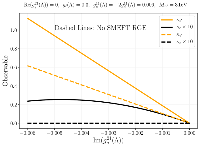
Figure 1: The dependence of $\kappa_{\epsilon}$ and $\kappa_{\epsilon^{\prime}}$ on Im$(g_{q}^{21})$ are shown. The Re$(q_{q}^{21})$ at scale $\Lambda$ is fixed to be zero. The diagonal quark and lepton couplings are fixed as discussed in the text. Further, the solid and dashed lines correspond to $Z^{\prime}$ with and without SMEFT RG running effects. The WET (QCD+QED) running is included in all cases.

In our scenario, at the scale of the $Z^{\prime}$ mass, the $\Delta F=2$ operators contributing to $\varepsilon_{K}$ are assumed to be suppressed. However, this assumption may not always hold at the low energy scales and the contributing operators might still be generated due to SMEFT RG running. We should make sure that this is not the case. At the high scale, we have the following four-quark operators

$$[{\cal O}_{qq}^{(1)}]_{2121} = (\bar{q}_{2}\gamma_{\mu}q_{1})(\bar{q}_{2}\gamma^{\mu}q_{1})\,,$$ (24)

$$[{\cal O}_{qd}^{(1)}]_{2111} = (\bar{q}_{2}\gamma_{\mu}q_{1})(\bar{d}_{1}\gamma^{\mu}d_{1})\,.$$ (25)

In our scenario, at the scale $\Lambda=M_{Z^{\prime}}$, the Wilson coefficient of the first operator is real and the second one is imaginary but it does not have the right flavour indices, so naively these operators should not affect $\varepsilon_{K}$. Through operator-mixing [44, 45], at the EW scale, in the leading-log approximation, we have

$$\Delta\big{[}{\cal C}_{qq}^{(1)}\big{]}_{2121}(M_{Z}) \approx {-}\frac{y_{t}^{2}}{16\pi^{2}}\left(\lambda_{t}^{22}\big{[}{\cal C}_{qq}^{(1)}\big{]}_{2121}(M_{Z^{\prime}})+\Lambda_{t}^{11}\big{[}{\cal C}_{qq}^{(1)}\big{]}_{2121}(M_{Z^{\prime}})\right)\log{\left(\frac{\Lambda}{M_{Z}}\right)}\,,$$ (26)

$$\Delta\big{[}{\cal C}_{qd}^{(1)}\big{]}_{2111}(M_{Z}) \approx {-}\frac{y_{t}^{2}}{16\pi^{2}}\left(\lambda_{t}^{22}\big{[}{\cal C}_{qd}^{(1)}\big{]}_{2111}(M_{Z^{\prime}})+\lambda_{t}^{11}\big{[}{\cal C}_{qd}^{(1)}\big{]}_{2111}(M_{Z^{\prime}})\right)\log{\left(\frac{\Lambda}{M_{Z}}\right)}\,,$$ (27)

here, $\lambda_{t}^{11}\approx 8.3\times 10^{-5},\lambda_{t}^{22}\approx 1.7\times 10^{-3}$. From the above two equations, it is clear that the RG running cannot induce the imaginary parts of $\big{[}{\cal C}_{qq}^{(1)}\big{]}_{2121}$ and $\big{[}{\cal C}_{qd}^{(1)}\big{]}_{2121}$ at $M_{Z}$.

Therefore, our initial assumptions are stable under the SMEFT RGEs. However, we still find a small effect in $\varepsilon_{K}$ due to the back-rotation effect [43], which is basically due to the running of the SM down-type Yukawa couplings. This is illustrated in Fig. 1. We observe that while the RG effects on $\varepsilon_{K}$ for this range of Im$(g_{q}^{21})$ are very small, they are large in the case of $\varepsilon^{\prime}/\varepsilon$.

3.3 Observables

In our numerical analysis we investigate the following quantities:

$$R_{\Delta M_{K}} = \frac{\Delta M_{K}^{BSM}}{\Delta M_{K}^{exp}}\,,\quad R_{\nu\bar{\nu}}^{+}=\frac{\mathcal{B}(K^{+}\to\pi^{+}\nu\bar{\nu})}{\mathcal{B}(K^{+}\to\pi^{+}\nu\bar{\nu})_{SM}}\,,\quad R_{\nu\bar{\nu}}^{0}=\frac{\mathcal{B}(K_{L}\to\pi^{0}\nu\bar{\nu})}{\mathcal{B}(K_{L}\to\pi^{0}\nu\bar{\nu})_{SM}}\,,$$ (28)

$$R_{\mu^{+}\mu^{-}}^{S} = \frac{\mathcal{B}(K_{S}\to\mu^{+}\mu^{-})_{\rm SD}}{\mathcal{B}(K_{S}\to\mu^{+}\mu^{-})^{SD}_{SM}}\,,\quad R_{\pi\ell^{+}\ell^{-}}^{0}=\frac{\mathcal{B}(K_{L}\to\pi^{0}\ell^{+}\ell^{-})}{\mathcal{B}(K_{L}\to\pi^{0}\ell^{+}\ell^{-})_{SM}}\,,\qquad\frac{\varepsilon^{\prime}}{\varepsilon}\,.$$

Relative to [13] the constraint from $\mathcal{B}(K_{L}\to\mu^{+}\mu^{-})$ can be avoided because there is no NP contribution to this decay in our scenario. In view of the recent progress in [46] on the extraction of the short-distance contribution to the $K_{S}\to\mu^{+}\mu^{-}$ branching ratio, we will compare this time NP contributions to the short-distance SM contribution and not to the full one that includes important long-distance effects.

4 Correlations between Kaon Observables: $|\kappa_{\varepsilon}|\leq 0.025$

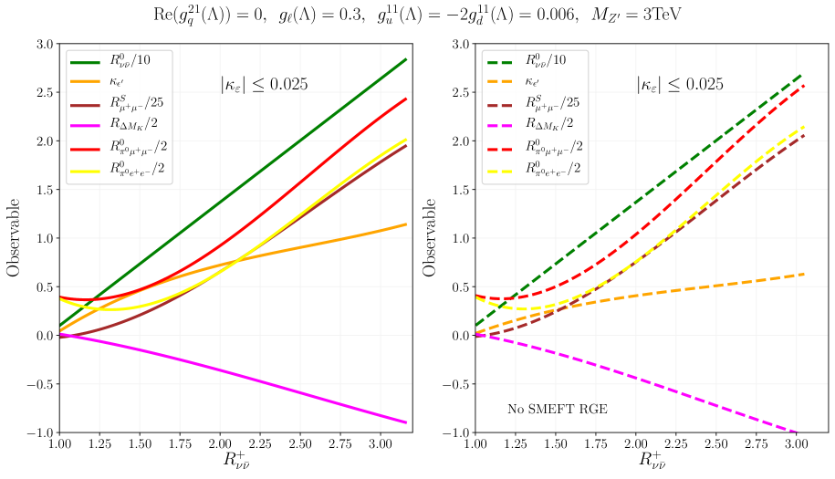
Figure 2: The correlations between the observable $R_{\nu\bar{\nu}}^{+}$ and various other Kaon observables are shown. The NP parameters are given in (29) and are the same as in Fig. 1.

In what follows we set the relevant $Z^{\prime}$ couplings at $\Lambda$ and its mass as in [13] to

$$g_{u}^{11}=-2g_{d}^{11}=6\times 10^{-3},\qquad g_{\ell}^{11}=g_{\ell}^{22}=0.3,\qquad M_{Z^{\prime}}=3~{}\,{\rm TeV}\,,$$ (29)

and

$$g_{u}^{11}=-2g_{d}^{11}=6\times 10^{-2},\qquad g_{\ell}^{11}=g_{\ell}^{22}=3.0,\qquad M_{Z^{\prime}}=10~{}\,{\rm TeV}\,,$$ (30)

for simplicity we define $g_{\ell}^{11}=g_{\ell}^{22}=g_{\ell}$. While the lighter $Z^{\prime}$ is still in the reach of the LHC, the heavier one can only be discovered at a future collider.

The relation between $g_{u}^{11}$ and $g_{d}^{11}$ assures that electroweak penguins are responsible for the possible enhancement of $\varepsilon^{\prime}/\varepsilon$ with respect to the SM value as expected within the Dual QCD approach [30].

For the numerical analysis the Python packages flavio[47], wilson [48] and WCxf [49] have been used, in which the complete matching of the SMEFT onto the WET [50, 51], as well as the full WET running [52, 53] are taken into account. Note that some of the observables such as $R_{\Delta M_{K}}$, $R^{0}_{\pi\ell^{+}\ell^{-}}$ are not implemented in the public version of flavio. For these we have used our private codes. In Fig. 1 we show that for $M_{Z^{\prime}}=3~{}\,{\rm TeV}$ with

$$-0.006\leq{\rm Im}(g_{q}^{21})\leq 0\,,$$ (31)

$\varepsilon^{\prime}/\varepsilon$ can indeed be significantly enhanced over its SM value while keeping the NP impact on $\varepsilon_{K}$ below $1\%$ of the experimental value. With the chosen quark couplings in (29) the negative values of ${\rm Im}(g_{q}^{21})$ are required to enhance $\varepsilon^{\prime}/\varepsilon$. For $M_{Z^{\prime}}=10~{}\,{\rm TeV}$ the quark and lepton couplings have to be increased to obtain similar effects. We observe significant RG effects in the case of $\varepsilon^{\prime}/\varepsilon$. Including them increases significantly the enhancement of $\varepsilon^{\prime}/\varepsilon$ for a given ${\rm Im}(g_{q}^{21})$. On the other hand this effect is very small in the case of $\varepsilon_{K}$.

An important test of this NP scenario will be the correlations between all observables discussed by us. This is illustrated in Figs. 2 and 3 for $M_{Z^{\prime}}=3~{}\,{\rm TeV}$ and $M_{Z^{\prime}}=10~{}\,{\rm TeV}$, respectively. We show there the dependence of various observables on the ratio $R_{\nu\bar{\nu}}^{+}$ restricting the values of ${\rm Im}(g_{q}^{21})$ to the range in (31) for which the NP effects in $\varepsilon_{K}$ are at most $1\%$. Of particular importance is the correlation between $R_{\nu\bar{\nu}}^{+}$ and $R_{\nu\bar{\nu}}^{0}$. As announced before the full action takes part exclusively on the MB branch parallel to the GN bound not shown in the plot. We observe a strong enhancement of $K_{L}\rightarrow\pi^{0}\nu\bar{\nu}$ branching ratio. Finding in the future the experimental values of both branching ratios outside the MB branch would indicate, among other possibilities, the presence of other particles which would affect ${\rm Re}X_{\rm eff}$. While the remaining correlations are self explanatory, let us make the following observations

• The four ratios in Fig. 2 and 3 that increase with increasing $R^{+}_{\nu\bar{\nu}}$ are very strongly correlated with each other because being CP-violating they depend only on ${\rm Im}(g_{q}^{21})$. While $\varepsilon^{\prime}/\varepsilon$ and $R_{\pi\mu^{+}\mu^{-}}^{0}$ can be significantly enhanced, the enhancements of $R_{\nu\bar{\nu}}^{0}$ and $R_{\mu^{+}\mu^{-}}^{S}$ are huge making hopes that even a moderate enhancement of $R_{\nu\bar{\nu}}^{+}$ over the SM prediction will allow to observe $K_{L}\rightarrow\pi^{0}\nu\bar{\nu}$ and $K_{S}\to\mu^{+}\mu^{-}$ in the coming years.

• The RG effects play a significant role in $\kappa_{\epsilon^{\prime}}$ and $R_{\Delta M_{K}}$ but otherwise these effects are small. RG effects are simply larger in non-leptonic decays than in semi-leptonic and leptonic ones.

The size of leptonic and semileptonic branching ratios depends on leptonic couplings but the correlations themselves do not depend on them because for left-handed couplings the couplings to charged leptons and neutrinos must be the same due to the unbroken $\text{SU(2)}_{L}$ symmetry in the SMEFT.

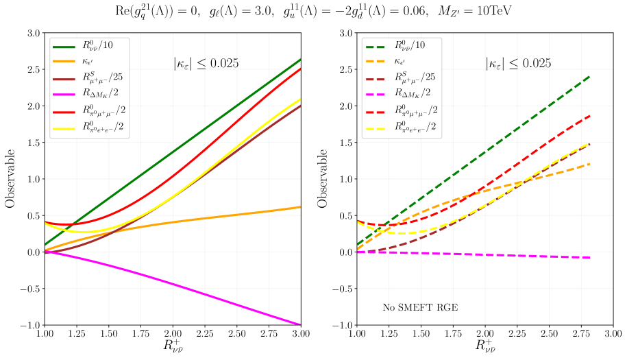
Figure 3: The correlations between the observable $R_{\nu\bar{\nu}}^{+}$ and various other Kaon observables are shown. The NP parameters and other details are the same as given in (30).

In order to illustrate the power of correlations we anticipate the future discovery of $Z^{\prime}$ with its mass $3\,{\rm TeV}$ and the measurement of NA62 collaboration resulting in

$$R_{\nu\bar{\nu}}^{+}=1.50\,.$$ (32)

For $g_{\ell}=0.3$ we find then

$$R_{\nu\bar{\nu}}^{0}\approx 7.5,\qquad\kappa_{\epsilon^{\prime}}\approx 0.5,\qquad R_{\mu^{+}\mu^{-}}^{S}\approx 5.0\,,$$ (33)

and

$$R_{\Delta M_{K}}\approx-0.25,\qquad R^{0}_{\pi^{0}\mu^{+}\mu^{-}}\approx 1.0\qquad R^{0}_{\pi^{0}e^{+}e^{-}}\approx 0.5.$$ (34)

Certainly, the results depend on the leptonic couplings. In the future they could be determined from other processes, in particular from B decays.

5 Summary and Outlook

In the present paper, we have demonstrated that despite the absence of NP in $\varepsilon_{K}$ large NP effects can be found in $K^{+}\rightarrow\pi^{+}\nu\bar{\nu}$, $K_{L}\rightarrow\pi^{0}\nu\bar{\nu}$, $K_{S}\to\mu^{+}\mu^{-}$, $K_{L}\to\pi^{0}\ell^{+}\ell^{-}$, $\varepsilon^{\prime}/\varepsilon$ and $\Delta M_{K}$. For this to happen the flavour changing coupling must be close to the imaginary one, reducing the number of free parameters. As the CKM parameters have been determined precisely from $\Delta F=2$ observables only [1], the paucity of NP parameters in this scenario implies strong correlations between all observables involved.

In the coming years, the most interesting will be an improved measurement of the $K^{+}\rightarrow\pi^{+}\nu\bar{\nu}$ branching ratio, which if different from the SM prediction will imply NP effects in the remaining observables considered by us. Figs. 2 and 3. illustrate this in a spectacular manner. The size of possible enhancements will depend on the involved couplings, in particular, leptonic ones so that correlations with $B$ physics observables will also be required to get the full insight into the possible anomalies. With improved theory estimates of $\varepsilon^{\prime}/\varepsilon$ and $\Delta M_{K}$, the improved measurements of $K_{L}\rightarrow\pi^{0}\nu\bar{\nu}$ and $K_{S}\to\mu^{+}\mu^{-}$, and those of $B$ decays, this simple scenario will undergo very strong tests.

Acknowledgements J.A. has received funding from the European Research Council (ERC) under the European Union’s Horizon 2020 research and innovation programme under grant agreement 833280 (FLAY), and by the Swiss National Science Foundation (SNF) under contract 200020 204428. Financial support for A.J.B from the Excellence Cluster ORIGINS, funded by the Deutsche Forschungsgemeinschaft (DFG, German Research Foundation), Excellence Strategy, EXC-2094, 390783311 is acknowledged. Research (J.K.) presented in this article was supported by the Laboratory Directed Research and Development program of Los Alamos National Laboratory under project number 20220706PRD1.

References

• [1] A. J. Buras and E. Venturini, The exclusive vision of rare K and B decays and of the quark mixing in the standard model, Eur. Phys. J. C 82 (2022), no. 7 615, [arXiv:2203.11960].
• [2] M. Bordone, B. Capdevila, and P. Gambino, Three loop calculations and inclusive $|V_{cb}|$, Phys. Lett. B 822 (2021) 136679, [arXiv:2107.00604].
• [3] Flavour Lattice Averaging Group (FLAG) Collaboration, Y. Aoki et al., FLAG Review 2021, Eur. Phys. J. C 82 (2022), no. 10 869, [arXiv:2111.09849].
• [4] A. J. Buras, Standard Model predictions for rare K and B decays without new physics infection, Eur. Phys. J. C 83 (2023), no. 1 66, [arXiv:2209.03968].
• [5] R. J. Dowdall, C. T. H. Davies, R. R. Horgan, G. P. Lepage, C. J. Monahan, J. Shigemitsu, and M. Wingate, Neutral $B$-meson mixing from full lattice QCD at the physical point, Phys. Rev. D 100 (2019), no. 9 094508, [arXiv:1907.01025].
• [6] J. Aebischer, A. J. Buras, and J. Kumar, On the Importance of Rare Kaon Decays: A Snowmass 2021 White Paper, in 2022 Snowmass Summer Study, 3, 2022. arXiv:2203.09524.
• [7] E. Goudzovski et al., Weak Decays of Strange and Light Quarks, arXiv:2209.07156.
• [8] J. Aebischer, Kaon physics overview, 12, 2022. arXiv:2212.09622.
• [9] M. Blanke, Insights from the Interplay of $K\rightarrow\pi\nu\overline{\nu}$ and $\epsilon_{K}$ on the New Physics Flavour Structure, Acta Phys.Polon. B41 (2010) 127, [arXiv:0904.2528].
• [10] Z. Bai, N. H. Christ, and C. T. Sachrajda, The $K_{L}$ - $K_{S}$ Mass Difference, EPJ Web Conf. 175 (2018) 13017.
• [11] B. Wang, Calculating $\Delta m_{K}$ with lattice QCD, PoS LATTICE2021 (2022) 141, [arXiv:2301.01387].
• [12] A. J. Buras, New physics patterns in $\varepsilon^{\prime}/\varepsilon$ and $\varepsilon_{K}$ with implications for rare kaon decays and $\Delta M_{K}$, JHEP 04 (2016) 071, [arXiv:1601.00005].
• [13] J. Aebischer, A. J. Buras, and J. Kumar, Another SMEFT story: $Z^{\prime}$ facing new results on $\epsilon^{\prime}/\epsilon$, $\Delta M_{K}$ and $K\to\pi\nu\overline{\nu}$, JHEP 12 (2020) 097, [arXiv:2006.01138].
• [14] J. Aebischer, A. J. Buras, M. Cerdá-Sevilla, and F. De Fazio, Quark-lepton connections in Z’ mediated FCNC processes: gauge anomaly cancellations at work, JHEP 02 (2020) 183, [arXiv:1912.09308].
• [15] A. J. Buras, F. De Fazio, and J. Girrbach, The Anatomy of Z’ and Z with Flavour Changing Neutral Currents in the Flavour Precision Era, JHEP 1302 (2013) 116, [arXiv:1211.1896].
• [16] A. J. Buras, F. De Fazio, J. Girrbach, and M. V. Carlucci, The Anatomy of Quark Flavour Observables in 331 Models in the Flavour Precision Era, JHEP 1302 (2013) 023, [arXiv:1211.1237].
• [17] G. Buchalla and A. J. Buras, The rare decays $K\to\pi\nu\bar{\nu}$, $B\to X\nu\bar{\nu}$ and $B\to\ell^{+}\ell^{-}$: An Update, Nucl. Phys. B548 (1999) 309–327, [hep-ph/9901288].
• [18] F. Mescia and C. Smith, Improved estimates of rare K decay matrix-elements from $K_{\ell 3}$ decays, Phys. Rev. D76 (2007) 034017, [arXiv:0705.2025].
• [19] A. J. Buras and E. Venturini, Searching for New Physics in Rare $K$ and $B$ Decays without $|V_{cb}|$ and $|V_{ub}|$ Uncertainties, Acta Phys. Polon. B 53 (9, 2021) A1, [arXiv:2109.11032].
• [20] Particle Data Group Collaboration, P. A. Zyla et al., Review of Particle Physics, PTEP 2020 (2020), no. 8 083C01.
• [21] Flavour Lattice Averaging Group Collaboration, S. Aoki et al., FLAG Review 2019: Flavour Lattice Averaging Group (FLAG), Eur. Phys. J. C 80 (2020), no. 2 113, [arXiv:1902.08191].
• [22] Y. Aoki et al., FLAG Review 2021, arXiv:2111.09849.
• [23] J. Brod, M. Gorbahn, and E. Stamou, Updated Standard Model Prediction for $K\to\pi\nu\bar{\nu}$ and $\epsilon_{K}$, 5, 2021. arXiv:2105.02868.
• [24] J. Brod, M. Gorbahn, and E. Stamou, Standard-model prediction of $\epsilon_{K}$ with manifest CKM unitarity, arXiv:1911.06822.
• [25] A. J. Buras, D. Guadagnoli, and G. Isidori, On $\epsilon_{K}$ beyond lowest order in the Operator Product Expansion, Phys. Lett. B688 (2010) 309–313, [arXiv:1002.3612].
• [26] A. J. Buras, M. Jamin, and P. H. Weisz, Leading and next-to-leading QCD corrections to $\varepsilon$ parameter and $B^{0}-\bar{B}^{0}$ mixing in the presence of a heavy top quark, Nucl. Phys. B347 (1990) 491–536.
• [27] J. Urban, F. Krauss, U. Jentschura, and G. Soff, Next-to-leading order QCD corrections for the $B^{0}-\bar{B}^{0}$ mixing with an extended Higgs sector, Nucl. Phys. B523 (1998) 40–58, [hep-ph/9710245].
• [28] Heavy Flavor Averaging Group (HFAG) Collaboration, Y. Amhis et al., Averages of b𝑏b-hadron, c𝑐c-hadron, and τ𝜏\tau-lepton properties as of summer 2016, arXiv:1612.07233. Updates on https://urldefense.com/v3/__http://www.slac.stanford.edu/xorg/hfag*7D*7Bhttp:/*www.slac.stanford.edu/xorg/hfag__;JSUv!!Mih3wA!WzHhMs_LrEEC6iOCPmeHL0di2Fuq19ujdL9vDWRi-hsLF8Wz-c-B5FHxeTo320oJWwbLq1dv$.
• [29] HFLAV Collaboration, Y. Amhis et al., Averages of $b$-hadron, $c$-hadron, and $\tau$-lepton properties as of 2021, arXiv:2206.07501.
• [30] A. J. Buras, $\varepsilon^{\prime}/\varepsilon$ in the Standard Model and Beyond: 2021, in 11th International Workshop on the CKM Unitarity Triangle, 3, 2022. arXiv:2203.12632.
• [31] J. Aebischer, C. Bobeth, and A. J. Buras, $\varepsilon^{\prime}/\varepsilon$ in the Standard Model at the Dawn of the 2020s, Eur. Phys. J. C 80 (2020), no. 8 705, [arXiv:2005.05978].
• [32] J. Aebischer, C. Bobeth, A. J. Buras, J.-M. Gérard, and D. M. Straub, Master formula for $\varepsilon^{\prime}/\varepsilon$ beyond the Standard Model, Phys. Lett. B792 (2019) 465–469, [arXiv:1807.02520].
• [33] J. Aebischer, C. Bobeth, A. J. Buras, and D. M. Straub, Anatomy of $\varepsilon^{\prime}/\varepsilon$ beyond the standard model, Eur. Phys. J. C79 (2019), no. 3 219, [arXiv:1808.00466].
• [34] J. Aebischer, A. J. Buras, and J.-M. Gérard, BSM hadronic matrix elements for $\epsilon^{\prime}/\epsilon$ and $K\to\pi\pi$ decays in the Dual QCD approach, JHEP 02 (2019) 021, [arXiv:1807.01709].
• [35] J. Aebischer, C. Bobeth, A. J. Buras, and J. Kumar, BSM master formula for $\varepsilon^{\prime}/\varepsilon$ in the WET basis at NLO in QCD, JHEP 12 (2021) 043, [arXiv:2107.12391].
• [36] C. Bobeth, A. J. Buras, A. Celis, and M. Jung, Patterns of Flavour Violation in Models with Vector-Like Quarks, JHEP 04 (2017) 079, [arXiv:1609.04783].
• [37] G. Isidori and R. Unterdorfer, On the short-distance constraints from $K_{L,S}\to\mu^{+}\mu^{-}$, JHEP 01 (2004) 009, [hep-ph/0311084].
• [38] G. D’Ambrosio and T. Kitahara, Direct $CP$ Violation in $K\to\mu^{+}\mu^{-}$, Phys. Rev. Lett. 119 (2017), no. 20 201802, [arXiv:1707.06999].
• [39] F. Mescia, C. Smith, and S. Trine, $K_{L}\to\pi^{0}e^{+}e^{-}$ and $K_{L}\to\pi^{0}\mu^{+}\mu^{-}$: A binary star on the stage of flavor physics, JHEP 08 (2006) 088, [hep-ph/0606081].
• [40] LHCb Collaboration, R. Aaij et al., Constraints on the $K^{0}_{S}\rightarrow\mu^{+}\mu^{-}$ Branching Fraction, Phys. Rev. Lett. 125 (2020), no. 23 231801, [arXiv:2001.10354].
• [41] KTEV Collaboration, A. Alavi-Harati et al., Search for the Decay $K_{L}\to\pi^{0}\mu^{+}\mu^{-}$, Phys. Rev. Lett. 84 (2000) 5279–5282, [hep-ex/0001006].
• [42] LHCb Collaboration, R. Aaij et al., Improved limit on the branching fraction of the rare decay ${{K}^{0}_{\mathrm{\scriptscriptstyle S}}}\rightarrow\mu^{+}\mu^{-}$, Eur. Phys. J. C77 (2017), no. 10 678, [arXiv:1706.00758].
• [43] J. Aebischer and J. Kumar, Flavour violating effects of Yukawa running in SMEFT, JHEP 09 (2020) 187, [arXiv:2005.12283].
• [44] E. E. Jenkins, A. V. Manohar, and M. Trott, Renormalization Group Evolution of the Standard Model Dimension Six Operators II: Yukawa Dependence, JHEP 01 (2014) 035, [arXiv:1310.4838].
• [45] R. Alonso, E. E. Jenkins, A. V. Manohar, and M. Trott, Renormalization Group Evolution of the Standard Model Dimension Six Operators III: Gauge Coupling Dependence and Phenomenology, JHEP 04 (2014) 159, [arXiv:1312.2014].
• [46] A. Dery, M. Ghosh, Y. Grossman, and S. Schacht, $K\rightarrow$ $\mu$+$\mu$ as a clean probe of short-distance physics, JHEP 07 (2021) 103, [arXiv:2104.06427].
• [47] D. M. Straub, flavio: a Python package for flavour and precision phenomenology in the Standard Model and beyond, arXiv:1810.08132.
• [48] J. Aebischer, J. Kumar, and D. M. Straub, Wilson: a Python package for the running and matching of Wilson coefficients above and below the electroweak scale, Eur. Phys. J. C78 (2018), no. 12 1026, [arXiv:1804.05033].
• [49] J. Aebischer et al., WCxf: an exchange format for Wilson coefficients beyond the Standard Model, Comput. Phys. Commun. 232 (2018) 71–83, [arXiv:1712.05298].
• [50] J. Aebischer, A. Crivellin, M. Fael, and C. Greub, Matching of gauge invariant dimension-six operators for $b\to s$ and $b\to c$ transitions, JHEP 05 (2016) 037, [arXiv:1512.02830].
• [51] E. E. Jenkins, A. V. Manohar, and P. Stoffer, Low-Energy Effective Field Theory below the Electroweak Scale: Operators and Matching, JHEP 03 (2018) 016, [arXiv:1709.04486].
• [52] J. Aebischer, M. Fael, C. Greub, and J. Virto, B physics Beyond the Standard Model at One Loop: Complete Renormalization Group Evolution below the Electroweak Scale, JHEP 09 (2017) 158, [arXiv:1704.06639].
• [53] E. E. Jenkins, A. V. Manohar, and P. Stoffer, Low-Energy Effective Field Theory below the Electroweak Scale: Anomalous Dimensions, JHEP 01 (2018) 084, [arXiv:1711.05270].