Transient stellar collisions as multimessenger probes:
Non-thermal-, gravitational wave emission and the cosmic ladder argument

Abstract

In dense stellar clusters like galactic nuclei and globular clusters stellar densities are so high that stars might physically collide with each other. In galactic nuclei the energy and power output can be close, and even exceed, to those from supernovae events. We address the event rate and the electromagnetic characteristics of collisions of main sequence stars (MS) and red giants (RG). We also investigate the case in which the cores form a binary and emit gravitational waves. In the case of RGs this is particularly interesting because the cores are degenerate. We find that MS event rate can be as high as tens per year, and that of RGs one order of magnitude larger. The collisions are powerful enough to mimic supernovae- or tidal disruptions events. We find Zwicky Transient Facility observational data which seem to exhibit the features we describe. The cores embedded in the gaseous debris experience a friction force which has an impact on the chirping mass of the gravitational wave. As a consequence, the two small cores in principle mimic two supermassive black holes merging. However, their evolution in frequency along with the precedent electromagnetic burst and the ulterior afterglow are efficient tools to reveal the impostors. In the particular case of RGs, we derive the properties of the degenerate He cores and their H-burning shells to analyse the formation of the binaries. The merger is such that it can be misclassified with SN Ia events. Because the masses and densities of the cores are so dissimilar in values depending on their evolutionary stage, the argument about standard candles and cosmic ladder should be re-evaluated.

1. Motivation

Dense stellar systems such as globular clusters and galactic nuclei have stellar densities ranging between a million and a hundred million stars per cubic parsec. In them, relative velocities of the order of $\sim\text{a~{}few~{}}10\,\text{km/s}$ in the case of globular clusters and of $\sim$ $100-1000\,\text{km/s}$ in the case of galactic nuclei can be reached (Neumayer et al. 2020; Spitzer 1987; Binney & Tremaine 2008). In these exceptional conditions, and unlike anywhere else in the host galaxy, collisional effects come into play. With “collisional” we mean in general mutual gravitational deflections which lead to an exchange of energy and angular momentum, but also in particular genuine contact collisions. The possibility that collisions between stars play a fundamental role both in explaining particular observations and in the global influence of dense stellar systems has been studied with dedicated numerical studies (Spitzer & Saslaw 1966; David et al. 1987a; Sanders 1970; Benz & Hills 1987; David et al. 1987b; Davies et al. 1991; Benz & Hills 1992; Murphy et al. 1991; Lai et al. 1993; Lombardi et al. 1995, 1996a; Bailey & Davies 1999a; Davies et al. 1998; Bailey & Davies 1999b; Lombardi et al. 2002a; Shara 2002; Adams et al. 2004; Trac et al. 2007; Dale et al. 2009; Wu et al. 2020; Mastrobuono-Battisti et al. 2021; Vergara et al. 2021).

We have chosen to first focus on galactic nuclei. We then address globular clusters, in which the rates are larger due to the smaller relative velocities between the stars participating in the collision (which is of the order of the velocity dispersion). For galactic nuclei, we first derive the event rate of these collisions as a function of the host galaxy cusp (section 2) and analyse analytically the non-thermal properties of the outcome of such collisions (sections 3 and 4). This analysis is performed for both main-sequence stars and, later, for red giants (section 6). The electromagnetic analysis reveals that these collisions can mimic over periods of time tidal disruptions but also Type Ia supernovae (da Silva 1993). Our analysis is a dynamical and analytical one, and depends on solely two free parameters which whose value should be extracted with dedicated numerical simulations.

We extend the analysis to the gravitational radiation phase as emitted by a subset of these collisions, namely those in which the core survives and forms a binary (section 5). Red giants have a very compact nucleus and can always withstand the onslaught of the collision.

We find that the number of gravitational wave sources that form is not negligible, and leads to the emergence of a type of source that can be misleading. A source that drastically changes its characteristics within a very short time. In a matter of months, the binary that forms initially appears to have a few solar masses to later appear as a supermassive black hole binary. Similarly, the luminosity distance varies tremendously in that short interval of time.

Due to the multi-messenger characteristics of this source, the extraction of information is very interesting and complementary. That is, electromagnetic data can help us to break various degeneracies in the analysis of gravitational waves and vice versa. In the particular case of the red giants, the rates are very high and, because the electromagnetic nature of the process very strongly depends on the stage of the evolution of the colliding red giants, if these collisions were confused with supernovae events, which are used as a kind of standard candles, the ladder argument to calculate cosmological distances would be in danger of revision.

Although galactic nuclei are often left out from the supernova searches, it is often difficult if not impossible to discern the nucleus due to a lack of resolution. Moreover, collisions happen more frequently in globular clusters, as mentioned before, which are located off the plane and away from the galactic nucleus, and are hence not excluded in the searches. However, the low relative velocities lead to a different kind of phenomenon: stellar pulsations. In Sec. (7) we find that the collisions in globular clusters can lead to the classical Cepheids pulsation phenomenon. We show that in the adiabatic, spherical case this is a stable phenomenon, and we calculate the associated timescale (sections 7.4 and 7.3). However, ulterior inputs of energy are required if the vibrational or thermal instability dissipate the oscillations. This additional inputs of energy can happen if futher collisions take place with the same companion star in the case of binary formation, or with another star, or in the case in which internal instabilities lead to them.

The classical pulsation problem has been envisaged as another rung in the standard candle classification of the cosmological ladder, so that this must be addressed in more detail than we present here, and will be presented elsewhere. We discuss the supernovae and pulsating star misclassification in the context of the cosmological ladder in Sec. (8).

Finally, in Sec. (9) we present a summary of all of the conclusions from our investigations.

2. Event rate derivation

The quasi-steady solution for how stars distribute around a massive black hole (MBH) follows an isotropic distribution function in physical space of the form $\rho(r)\sim R^{-\gamma}$, where $\rho$ is the stellar density $\rho$ and $R$ the radius (Peebles 1972; Bahcall & Wolf 1976). This mathematical derivation has been corroborated using numerical techniques (Shapiro & Marchant 1978; Marchant & Shapiro 1979, 1980; Shapiro & Teukolsky 1985; Freitag & Benz 2001; Amaro-Seoane et al. 2004; Preto et al. 2004) and, recently, a comparison with data from our Galactic Centre yields a very good match between observations, theory and numerical simulations (Baumgardt et al. 2018; Gallego-Cano et al. 2018; Schödel et al. 2018).

Therefore, we assume a power-law mass distribution for the numerical density of stars around the MBH, $n_{*}(R)\propto R^{-\gamma}$, with $R$ the radius. Following this, we can derive that the enclosed stellar mass around the MBH within a given radius is (see e.g. Amaro-Seoane 2019)

$$M_{*}(R)=M_{\bullet}\left(\frac{R}{R_{\rm infl}}\right)^{3-\gamma}.$$ (1)

In this last equation $M_{*}(R)$ is the stellar mass at a radius $R$, $M_{\bullet}$ is the mass of the MBH, $R_{\rm infl}$ is the influence radius of the MBH (i.e. the radius within which the potential is dominated by the MBH) and $\gamma$ is the exponent of the power law. Hence, the total number of stars at that radius is

$$N_{*}(R)=\frac{M_{\bullet}}{m_{*}}\left(\frac{R}{R_{\rm infl}}\right)^{3-\gamma},$$ (2)

where $m_{*}$ is the mass of one star and we are assuming for simplicity that all stars have the same mass and radius $R_{*}$, so that the stellar mass density at a given radius is $\rho_{*}(R)=m_{*}\,n_{*}(R)$. Therefore, we have that the numerical density is

$$n_{*}(R)=\frac{3-\gamma}{4\pi}\frac{M_{\bullet}}{m_{*}R_{\rm infl}^{3}}\left(\frac{R}{R_{\rm infl}}\right)^{-\gamma},$$ (3)

since $dN_{*}/dR=4\pi R^{2}\,n_{*}$.

At the radii of interest, those close to the MBH, within the radius of influence, the typical relative velocity between stars

$$V_{\rm rel}(R)=K_{v}\sqrt{\frac{GM_{\bullet}}{R}}$$ (4)

is $V_{\rm rel}(R)\geqslant V_{\rm esc}$, with $V_{\rm esc}$ the escape velocity from the stellar surface,

$$V_{\rm esc}=\sqrt{\frac{2Gm_{*}}{R_{*}}},$$ (5)

and $K_{v}$ depends on $\gamma$ and is of order unity.

The collision rate for one star can be estimated as

$$\frac{1}{T_{{\rm coll},\,1}(R)}=n_{*}(R)\,V_{\rm rel}(R)\,S,$$ (6)

with $S$ the cross-section,

$$S=\pi\left(f_{\rm coll}2R_{*}\right)^{2},$$ (7)

since we are neglecting the gravitational focusing, because $V_{\rm rel}(R)\geqslant V_{\rm esc}$, so that $S$ can be computed geometrically. In practise this means that we are looking at a lower-limit case, since the rates could be slightly enhanced. This is particularly true in globular clusters, where the relative velocity is lower. As stated in the introduction, nonetheless, we are focusing in galactic nuclei, which is a lower-limit case of the general scenario. In this equation, $f_{\rm coll}$ defines how deep a collision is.

Introducing Eq. (7), $n_{*}(R)$ and $V_{\rm rel}(R)$ in Eq. (6), we have that

$$\frac{1}{T_{{\rm coll},\,1}(R)}=(3-\gamma)K_{v}f_{\rm coll}^{2}\left(\frac{R_{*}}{R_{\rm infl}}\right)^{2}\frac{M_{\bullet}}{m_{*}}\sqrt{\frac{GM_{\bullet}}{R_{\rm infl}^{3}}}\left(\frac{R}{R_{\rm infl}}\right)^{-(\gamma+1/2)}$$ (8)

The total collisional rate in the cusp around the MBH is

$$\Gamma_{\rm coll}=\frac{N_{*}}{2}\frac{1}{T_{\rm coll,\,tot}},$$ (9)

since $N_{*}=4\pi R^{2}n_{*}$ and we take into account that for a collision we need two stars. Therefore

$$\Gamma_{\rm coll}=2\pi\int^{R_{\rm max}}_{R_{\rm min}}n_{*}(R)\frac{R^{2}}{{T_{\rm coll,\,1}(R)}}dR.$$ (10)

In this integral we choose the maximum radius $R_{\rm max}$ to be the distance within the influence radius at which $V_{\rm rel}(R)=V_{\rm esc}(R)$, i.e.

$$R_{\rm max}=K_{v}^{-2}R_{*}\frac{M_{\bullet}}{m_{*}},$$ (11)

and the minimum radius $R_{\rm min}$ to be the radius which contains on average one star. From Eq. (2) we derive that

$$R_{\rm min}=R_{\rm infl}\left(\frac{m_{*}}{M_{\bullet}}\right)^{\frac{1}{3-\gamma}}.$$ (12)

We note that the interior mass enclosed in $R_{\rm max}$ is

$$M_{*,\,{\rm max}} =K_{v}^{-2(3-\gamma)}M_{\bullet}\left(\frac{R_{*}}{R_{\rm infl}}\right)^{3-\gamma}\left(\frac{M_{\bullet}}{m_{*}}\right)^{3-\gamma}\approx$$

$$M_{\bullet}\left(\frac{\sigma_{v}^{2}}{V_{\rm esc}^{2}}\right)\ll M_{\bullet},$$ (13)

where $\sigma_{v}$ is the velocity dispersion at large distances from the MBH. This last equation means that $R_{\rm max}\ll R_{\rm infl}$.

We can now integrate Eq. (10),

$$\Gamma_{\rm coll} =2.12\times 10^{-9}\frac{1}{yr}\frac{(3-\gamma)^{2}}{5-4\gamma}K_{v}\left(\frac{f_{\rm coll}}{0.25}\right)^{2}\left(\frac{R_{*}}{1\,R_{\odot}}\right)^{2}\times$$

$$\left(\frac{M_{\bullet}}{10^{6}M_{\odot}}\right)^{5/2}\left(\frac{m_{*}}{1\,M_{\odot}}\right)^{-2}\left(\frac{R_{\rm infl}}{1\,\textrm{pc}}\right)^{-7/2}\times$$

$$\left[A(\gamma)\left(\frac{R_{*}}{R_{\odot}}\right)^{-2\gamma+5/2}\left(\frac{M_{\bullet}}{10^{6}M_{\odot}}\right)^{-2\gamma+5/2}\left(\frac{R_{\rm infl}}{1\textrm{pc}}\right)^{2\gamma-5/2}\times\right.$$

$$\left.\left(\frac{m_{*}}{1\,M_{\odot}}\right)^{2\gamma-5/2}-B(\gamma)\left(\frac{M_{\bullet}}{10^{6}M_{\odot}}\right)^{\frac{2\gamma-5/2}{3-\gamma}}\left(\frac{m_{*}}{1\,M_{\odot}}\right)^{\frac{5/2-2\gamma}{3-\gamma}}\right],$$ (14)

where we have defined

$$A(\gamma):= 2.25^{-2\gamma+5/2}10^{4\gamma-5}K_{v}^{4\gamma-5}$$

$$B(\gamma):= 10^{\frac{12\gamma-15}{3-\gamma}}$$ (15)

We note that, since $R_{\rm min}\ll R_{\rm max}$, the rates are dominated at short distances from the MBH, so that the first term in the square brackets of Eq. (14) can in principle be neglected. However, since this could artificially increase the rates, we do not neglect it. We have normalised $f_{\rm coll}$ to $0.25$ because we are interested in collisions which lead to a total disruption of the stars. This situation is achieved when the periastron distance of a gravitational two-body hyperbolic encounter in the centre-of-mass reference frame $d_{\rm min}$ has the value

$$d_{\rm min}=\left(R_{{\rm half},1}+R_{{\rm half},2}\right),$$ (16)

with $R_{{\rm half},1}$ the half-mass radius of the first star participating in the collision (and $R_{{\rm half},1}=R_{{\rm half},2}$ since we assume they have the same radius and mass). Therefore, for a complete disruptive collision $f_{\rm coll}$, a measure of the depth of the impact, as we explained, is

$$f_{\rm coll}\approx\frac{R_{\rm half}}{R_{*}}.$$ (17)

As we can see in e.g. Fig. 4 of Freitag & Benz (2005) (and see also their Fig. 9), for $m_{*}=1\,M_{\odot}$, $R_{*}=1\,R_{\odot}$, and then $f_{\rm coll}=0.25$. For $m_{*}=10\,M_{\odot}$, $R_{*}=6\,R_{\odot}$, and $f_{\rm coll}=0.2$

As for the influence radius, we use the so-called “mass-sigma” correlation (McConnell et al. 2011; Kormendy & Ho 2013; Davis et al. 2017) for black hole masses in nearby galaxies,

$$\frac{M_{\bullet}}{3\times 10^{8}\,M_{\odot}}\cong\left(\frac{\sigma}{200\,\textrm{km\,s}^{-1}}\right)^{5},$$ (18)

with $\sigma$ the velocity dispersion of the stars. This combined with the definition of the influence radius which takes into account the overall effect on the motion of a star by the bulge, including those that have moved away from the MBH, as introduced by Peebles (1972),

$$R_{\rm infl}=\frac{G\,M_{\bullet}}{\sigma^{2}},$$ (19)

leads to

$$R_{\rm infl}=1.05\,\textrm{pc}\times\left(\frac{M_{\bullet}}{10^{6}\,M_{\odot}}\right)^{0.6},$$ (20)

and note that for $M_{\bullet}=4\times 10^{6}\,M_{\odot}$ such as the one in our Galactic Centre, $R_{\rm infl}=2.5\,\textrm{pc}$, which is close to the value observed of $\sim 3\textrm{pc}$ (Schödel et al. 2014, 2018). Hence, for $M_{\bullet}=10^{7}\,M_{\odot}$, $R_{\rm infl}=4.2\,\textrm{pc}$ and for $M_{\bullet}=10^{5}\,M_{\odot}$, $R_{\rm infl}=0.27\,\textrm{pc}$.

For a Bahcall-Wolf power-law (Bahcall & Wolf 1976), $\gamma=7/4$, taking $f_{\rm coll}=0.25$, and the default values given in Eq. (14), we obtain that $\Gamma_{{\rm coll},\,6}\cong 10^{-4}\textrm{yr}^{-1}$ for a Milky-Way-like nucleus, i.e. with a MBH in this mass range, $M_{\bullet}=10^{6}\,M_{\odot}$ (as indicated with the sub-index 6).

The calculation of the event rate applies to nuclei hosting MBHs with masses between $\sim 10^{5}-10^{7}\,M_{\odot}$ , since for larger MBH masses the relaxation time would exceed a Hubble time, and for lighter MBH masses the MBH is in the intermediate-mass regime and hence cannot be envisaged as fixed in the centre of the potential, but wandering, which renders the calculation much more complicated. For $M_{\bullet}=10^{7}\,M_{\odot}$, and taking the same parameters as for the $M_{\bullet}=10^{6}\,M_{\odot}$ case but for the influence radius, we obtain that $\Gamma_{{\rm coll},\,7}\cong 2\times 10^{-4}\textrm{yr}^{-1}$, and for $M_{\bullet}=10^{5}\,M_{\odot}$, $\Gamma_{{\rm coll},\,5}\cong 10^{-5}\textrm{yr}^{-1}$.

Assuming an observable distance of $100\,\textrm{Mpc}$ for these events, this translates into an observable volume of $\sim 4.2\times 10^{6}\,\textrm{Mpc}^{3}$. Within this volume, and assuming $10^{-2}$ MBH of $M_{\bullet}=10^{6}\,M_{\odot}$ per $\textrm{Mpc}^{3}$ (see Fig.2 of Kelly & Merloni 2012), we derive a total of $4.2\times 10^{4}$ sources, i.e. nuclei hosting MBHs with a mass of $M_{\bullet}=10^{6}\,M_{\odot}$, so that this multiplied by $\Gamma_{{\rm coll},\,6}$ leads to a total event rate of $\Gamma_{{\rm coll},\,6}^{\rm tot}\sim 4.2\,\textrm{yr}^{-1}$. For MBHs with masses of $10^{7}\,M_{\odot}$, the work of Kelly & Merloni (2012) yields $6\times 10^{-3}$ MBH per $\textrm{Mpc}^{3}$, and hence $\Gamma_{{\rm coll},\,7}^{\rm tot}\sim 5\,\textrm{yr}^{-1}$. For MBHs with masses of $10^{5}\,M_{\odot}$, and extrapolating the results of Kelly & Merloni (2012), to about $10^{-2}$ MBH per $\textrm{Mpc}^{3}$ as well, we have that $\Gamma_{{\rm coll},\,5}^{\rm tot}\sim 0.42\,\textrm{yr}^{-1}$. Therefore, neglecting the contribution of $10^{5}\,M_{\odot}$ MBHs, and for a mass range for the MBH between $[10^{6},\,\textrm{a~{}few\,}10^{7}]\,M_{\odot}$, we have a total integrated event rate of $\gtrsim 100\textrm{\,yr}^{-1}$ in $100\,\textrm{Mpc}$. In Fig.(1) we show $\Gamma_{{\rm coll},\,6}^{\rm tot}$ and $\Gamma_{{\rm coll},\,7}^{\rm tot}$ for various typical values of $\gamma$ in a volume of $100\,\textrm{Mpc}$ of radius.

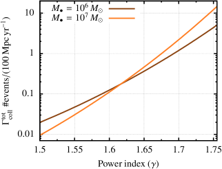
Figure 1.— Total amount of events per year in a volume of $100\,\textrm{Mpc}$ of radius for two different values of MBHs and for typical values of the power index $\gamma$. We note that $\gamma=1.75$ corresponds to the theoretical expectation of a relaxed nucleus for a single-mass population (Peebles 1972; Bahcall & Wolf 1976). We show lower values as an illustration for the dependency of $\Gamma_{{\rm coll}}^{\rm tot}$ with $\gamma$, which is not obvious from Eq. (14). At smaller values of $\gamma$, $10^{6}\,M_{\odot}$ is the upper curve and from $\gamma\sim 1.625$ the situation reverts and the upper one corresponds to $10^{7}\,M_{\odot}$.

3. Energy release

During the collision release of nuclear energy is negligible (see Mathis 1967; Różyczka et al. 1989). Gravitational energy can also be neglected in the kind of collisions we are considering (very high velocities and $f\sim 0.2$). We can also neglect radiative transport, since the merging stars are obviously optically thick while the collision it taking place. During it, the energy transport by radiation is diffusive.

In this kind of almost head-on stellar collisions and in our framework of high relative velocities, the colliding stars merge into a single object surrounded by a gaseous structure which is approximately spherical (see e.g. the numerical work of Freitag & Benz 2005). This gaseous cloud will expand at a speed which is equivalent to the average relative speeds one observes at galactic centres harbouring MBHs of masses $M_{\bullet}=[10^{6},\,\textrm{a~{}few}\,10^{7}]\,M_{\odot}$.

In this section, we first estimate the timescale for the energy to diffuse from the centre of the cloud to the surface and the timescale associated for the cloud to become transparent. Then we calculate the total emission of the energy and its time dependency, as well as the luminosity.

3.1. Diffusion of energy: Timescales

We estimate the associated timescales for a cloud to diffuse energy to the surface and for it to become fully transparent. We consider it to be transparent when the mean free path of photons is larger than the radius of the cloud.

We define the mean free path $l(t)$ (which changes over time) as the average distance for a photon between two interactions with two electrons at a given time, so that the time to cover it is $l(t)/c$, with $c$ the speed of light. Since we are talking about a random-walk process, the average number of steps of length $l(t)$ for the photon to cover a distance $R(t)$ (the radius of the cloud, function of time) is

$$N(t)=\left(\frac{R(t)}{l(t)}\right)^{2},$$ (21)

because the average of the squared distance is proportional to the time in a random walk.

We define the diffusion time as this number of steps multiplied by the time to cover the distance between two interactions, so that

$$T_{\rm diff}(t)\cong\frac{N(t)\,l(t)}{c}.$$ (22)

We now calculate the mean free path by estimating the probability $P_{\rm coll}$ that an electron collides with a photon after a distance $x$,

$$dP_{\rm coll}=S_{\rm eff}\,n\,dx,$$ (23)

with $S_{\rm eff}$ is the effective area and $n$ the numerical density of electrons. Hence, the collisional rate for one electron is

$$\Gamma_{\rm e}=\frac{dP_{\rm coll}}{dt}=S_{\rm eff}\,n\,v,$$ (24)

with $v$ the relative velocity between the electron and the photon, i.e. $v=c$. Therefore, the average number of collisions over a distance $x$ is

$$N_{\rm coll}=S_{\rm eff}\,n\,x.$$ (25)

By setting $N_{\rm coll}=1$ in this last equation, we derive the value of $x$, i.e. the mean free path,

$$l=\frac{1}{S_{\rm eff}\,n}.$$ (26)

Since $n=\rho_{\rm g}/m$, with $m$ the mass of one “gas particle” (i.e. the proton mass, since we assume that we have completly ionised H) per electron,

$$l=\frac{m}{\rho_{\rm g}\,S_{\rm eff}},$$ (27)

which allows us to introduce the usual definition of opacity, $\kappa=S_{\rm eff}/m$. If we assume that the ionisation degree does not change, then $l\propto 1/\rho_{\rm g}$, and since $\rho_{\rm g}\simeq M/R(t)^{3}$, we derive that $l(t)\propto R(t)^{3}$. Therefore, there must be a time in which $l(t)>R(t)$ and the cloud is transparent, $t=t_{\rm transp}$. If at that moment, which we denote as $t=t_{\rm transp}$, there is still enough energy in form of photons in the cloud, they will be able to escape it instantaneously even if they are located at the centre of the cloud, in a straight line, without diffusion.

I.e. if $t$ is the time passed since the formation of the cloud (i.e. right after the collision), and $T_{\rm diff}\ll t$, then most of the photons are still trapped in the cloud. Nonetheless, $t$ obviously increases and $T_{\rm diff}$ varies in time, so that there might be a moment in which $t>T_{\rm diff}$ before we reach $t=t_{\rm transp}$. We need to estimate these timescales. From the previous equations, we have that

$$T_{\rm diff}(t)\simeq\frac{\kappa}{c}\frac{M}{R(t)}.$$ (28)

With $\kappa=0.04\,\textrm{m}^{2}\textrm{kg}^{-1}$ (a lower bound for an ionised gas due to electron scattering). In the right hand side of this last equation everything is constant but for $R(t)$, which increases, so that $T_{\rm diff}(t)$ decreases with time. We can calculate at what time $T_{\rm diff}$ is reached, so as to compare it with $t=t_{\rm transp}$. An approximation is to set $T_{\rm diff}=t$ in Eq. (28), so that if we approximate the expansion velocity $V_{\rm exp}$ to the relative velocity, $V_{\rm exp}=10^{4}\,\textrm{km\,s}^{-1}$ (we will elaborate on this choice later), we have that $t=\sqrt{\kappa M/(V_{\rm exp}c)}$. Hence,

$$T_{\rm diff}\sim 0.16\,\textrm{yrs}\sim 2\,\textrm{months}$$ (29)

After reaching this time, approximately half of the total energy contained in the cloud has been released and the remaining half is still trapped in it. If we wait two times this amount of time, half of half the initial energy will still be in the cloud, so that the remaining amount of energy in the cloud goes as $1/2^{n}$ the initial amount, with $n$ the amount of temporal intervals corresponding to $T_{\rm diff}$. We note that this assumes that $T_{\rm diff}(t)$ is the same as $T_{\rm diff}(0)$. This is of course not true but it gives us a first rough estimate of the initial timescale for half of the energy to be released. We will improve this approximation in Sec. (3.3).

To calculate at what time $t_{\rm transp}$ is reached, we substitute $R(t)=l(t)$, so that,

$$R(t)\simeq\sqrt{\kappa\,M}.$$ (30)

Adopting the same values as before, we find that $t_{\rm transp}\sim 9\,\textrm{yr}$. When the cloud has become transparent, all of the energy will have been already radiated away via diffusion.

3.2. Total emission of energy

The total energy involved in the collision $E_{\rm tot}$ is the sum of three contributions: The binding energy of the stars ($E_{\rm bin}$) which take place in the collision plus the kinetic energy $E_{\rm kin}$ at infinity. For one of the stars participating in the collision, these values are

$$E_{\rm kin} =\frac{\mu}{2}V_{\rm rel}^{2}$$

$$E_{\rm bin} =\alpha\frac{Gm_{*}^{2}}{R_{*}},$$ (31)

with $\mu:=m_{*,\,1}m_{*,\,2}/(m_{*,\,1}+m_{*,\,2})$ the reduced mass, and $\alpha=3/(5-n)$, with $n=3$ for a Sun-like star (see Chandrasekhar 1942, for the equation and value). We can approximate $E_{\rm bin}\approx m_{*}V_{\rm esc}^{2}$, so that for the two stars

$$E_{\rm tot}\approx-\left(m_{*,\,1}V_{\rm esc,\,1}^{2}+m_{*,\,2}V_{\rm esc,\,2}^{2}\right)+{\mu}V_{\rm rel}^{2}.$$ (32)

As mentioned in Sec. (2), since $R_{\rm min}\ll R_{\rm max}$, the collisional rate will be dominated at smaller radii. For $M_{\bullet}=10^{6}\,M_{\odot}$, and for the adopted value of $\gamma=7/4$, Eq. (12) yields $R_{\rm min}\sim 10^{-5}\textrm{pc}$, so that $V_{\rm rel}\cong 20000\textrm{km\,s}^{-1}$. One order of magnitude farther away from the centre in radius, at $10^{-4}\textrm{pc}$, $V_{\rm rel}\cong 6500\textrm{km\,s}^{-1}$. For $M_{\bullet}=10^{7}\,M_{\odot}$, the minimum radius is also $R_{\rm min}\sim 10^{-5}\textrm{pc}$ but $V_{\rm rel}\cong 65000\textrm{km\,s}^{-1}$. At a distance from the MBH of $\sim 10^{-4}\textrm{pc}$ $V_{\rm rel}\cong 20000\textrm{km\,s}^{-1}$.

At such high relative velocities, we can ignore the contribution of the binding energy of the stars in Eq. (32). To consider two limiting cases, a $M_{\bullet}=10^{7}\,M_{\odot}$ at $R_{\rm min}\sim 10^{-5}\textrm{pc}$, yields $E_{\rm tot}\approx 42\,\textrm{foe}$ ($4.2\times 10^{52}\textrm{ergs}$), while a $M_{\bullet}=10^{6}\,M_{\odot}$ at a distance of $10^{-4}\textrm{pc}$ yields $E_{\rm tot}\approx 0.42\,\textrm{foe}$ ($4.2\times 10^{50}\textrm{ergs}$). A “typical” case would range between these two limits; i.e. $E_{\rm tot}\approx 1\,\textrm{foe}$, which is the usual energy release of a supernova (considering $V_{\rm rel}\cong 10000\textrm{km\,s}^{-1}$ at $10^{-4}\textrm{pc}$).

3.3. Time evolution of the released energy and power

We define the loss of energy in the cloud as

$$\frac{dE}{dt}=-\frac{E}{T_{\rm diff}(t)},$$ (33)

with $T_{\rm diff}(t)$ as given by Eq. (28). The physical meaning of the last equation is that we are identifying $T_{\rm diff}(t)$ as the time for the photons to escape the cloud as the main sink of energy of it and, hence, the right hand side is negative. Therefore,

$$\frac{dE}{E}=-\frac{1}{\xi}\,t\,dt,$$ (34)

with $\xi^{-1}:=cV_{\rm exp}/(\kappa M)$. The solution to Eq. (34) is

$$E(t)=E(0)\left(\frac{\eta}{1}\right)\exp{\left[-\frac{1}{2\,\xi}t^{2}\right]}.$$ (35)

Here $\eta$ is a parameter quantifying the amount of initial kinetic energy $E(0)$ that goes into radiation. The value of $\eta$ depends on the details of the collision and in particular on the slowing down of the shock downstreams; i.e. how the shock evolves during the collision will alter the relative velocity of the parts of the stars which have still not collided and translate into a total efficiency conversion of the kinetic into radiation. See for instance the work of Calderón et al. (2020), in particular their Figs. 4-10. In this work they focus on relatively low velocities and stellar winds but it illustrates the non-linearity of our problem. The derivation of this parameter requires detailed numerical simulations.

We now introduce

$$T_{\rm E}\equiv\sqrt{\frac{\kappa\,M}{c\,V_{\rm exp}}}=\sqrt{T_{\rm diff}(0)\frac{R(0)}{V_{\rm exp}}},$$ (36)

as we can see from Eq. (28). This corresponds to $t$ in the approximation we did before, to obtain Eq. (29). Indeed, for the values we adopted to derive Eq. (29), we have that $T_{\rm E}=0.16\,\textrm{yr}$. We can now rewrite Eq. (34) as

$$E(t)=E(0)\left(\frac{\eta}{1}\right)\exp{\left[-\frac{1}{2}\,\left(\frac{t}{T_{\rm E}}\right)^{2}\right]}.$$ (37)

Normalizing to standard values, we have

$$E(t)=10^{51}\,\textrm{ergs}\left(\frac{E(0)}{10^{51}\,\textrm{ergs}}\right)\left(\frac{\eta}{1}\right)\exp\left[-\frac{1}{8}\left(\frac{t}{1\,\textrm{month}}\right)^{2}\right].$$ (38)

In Fig.(2) we depict this time evolution for an initial energy of $E(0)=10^{51}\,\textrm{ergs}$.

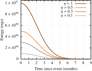
Figure 2.— Time evolution of the released energy for four different values of $\eta$, ranging from $1$ (uppermost curve) to $0.1$ (lowest curve).

With Eq. (37) we can obtain the emitted power by deriving this last equation,

$$P(t)=-\frac{dE}{dt}=\frac{E(0)}{T_{\rm E}^{2}}\,\left(\frac{\eta}{1}\right)\,t\,\exp\left[-\frac{1}{2}\,\left(\frac{t}{T_{\rm E}}\right)^{2}\right].$$ (39)

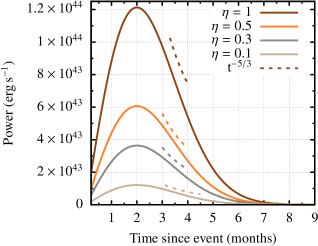
Figure 3.— Evolution of the power by a stellar disruption of masses $1\,M_{\odot}$ and $V_{\rm rel}=10^{4}\,\textrm{km\,s}^{-1}$, corresponding to the default values of Eq. (43) for different efficiency parameters $\eta$. The uppermost curve corresponds to the maximum value of $\eta$ and the lowermost to the minimum value. We add a power-law curve proportional to $t^{-5/3}$, which is the typical value one expects from a stellar tidal disruption.

We can normalize the equations by defining $\tau:=t/T_{\rm E}$ and $P_{\rm norm}\equiv E(0)/T_{\rm E}$, so that

$$E(\tau) =E(0)\,\left(\frac{\eta}{1}\right)\,\exp\left[-\frac{\tau^{2}}{2}\right]$$ (40)

$$P(\tau) =P_{\rm norm}\,\tau\,\left(\frac{\eta}{1}\right)\,\exp\left[-\frac{\tau^{2}}{2}\right].$$ (41)

We note here that $\tau$ contains the information relative to the scattering length of the environment, in $\kappa$, since the mean free path $l=1/(\rho_{\rm g}\,\kappa)$, as we can see in Eq. (26), so that encoded in $T_{\rm E}$ in Eq. (37) we have the information about the location of the peak of the distribution, which is, as we derived, after $2$ months.

Adopting typical values, we can express $P_{\rm norm}$ as follows,

$$P_{\rm norm}\cong\times 10^{44}\,\textrm{erg\,s}^{-1} \left(\frac{E(0)}{10^{51}\,\textrm{ergs}}\right)\left(\frac{\kappa}{0.04\,\textrm{m}^{2}\textrm{kg}^{-1}}\right)^{-1/2}$$

$$\left(\frac{M}{1\,M_{\odot}}\right)^{-1/2}\left(\frac{V_{\rm exp}}{10^{4}\textrm{km\,s}^{-1}}\right)^{1/2}.$$ (42)

Therefore, the final equation for the evolution of power with time is

$$P(t)\cong 10^{44}\textrm{erg\,s}^{-1} \left(\frac{\eta}{1}\right)\left(\frac{t}{1\,\textrm{month}}\right)\exp\left[-\frac{1}{8}\left(\frac{t}{1\,\textrm{month}}\right)^{2}\right]$$

$$\left(\frac{E(0)}{10^{51}\,\textrm{ergs}}\right)\left(\frac{\kappa}{0.04\,\textrm{m}^{2}\textrm{kg}^{-1}}\right)^{-1/2}$$

$$\left(\frac{M}{1\,M_{\odot}}\right)^{-1/2}\left(\frac{V_{\rm exp}}{10^{4}\textrm{km\,s}^{-1}}\right)^{1/2}.$$ (43)

In Fig. (3) we depict this power for various values of $\eta$. Decreasing $\eta$ shifts the peak of the power, lowers its maximum and broadens the distribution, as expected from Eq. (33). We have added a line which follows a power-law of time, $t^{-5/3}$, which corresponds to a stellar tidal disruption (see e.g. Rees 1988). If the observation of the event takes place between the 3rd and 4th month after the collision, it could easily be misinterpreted as a tidal disruption. At later times the curves diverge, so that depending on the observational errors one could discern the two, or not.

4. Temperature and spectral power

4.1. Effective temperature

From the previous section, we can now estimate the evolution of the effective temperature of the cloud which expands at a constant velocity $V_{\rm exp}$. We use the approximation of Stefan–Boltzmann of black body radiation, $P(t)=\sigma\,T_{\rm eff}^{4}\,4\pi R(t)^{2}$, with $\sigma$ the Stefan–Boltzmann constant and $T_{\rm eff}$ the effective temperature of the body, and assume that the radius of the cloud coincides with the photosphere. The physical interpretation of the definition of this temperature corresponds to the observed temperature, i.e. what a telescope would measure from the moment of the impact onwards.

From Eq. (43) we obtain

$$T_{\rm eff} \cong 2.32\times 10^{6}\,\textrm{K}\left(\frac{\eta}{1}\right)^{1/4}\left(\frac{t}{1\,\textrm{month}}\right)^{1/4}\exp\left[-\frac{1}{2}\left(\frac{t}{1\,\textrm{month}}\right)^{2}\right]$$

$$\left(\frac{E(0)}{10^{51}\,\textrm{ergs}}\right)^{1/4}\left(\frac{\kappa}{0.04\,\textrm{m}^{2}\textrm{kg}^{-1}}\right)^{-1/8}\left(\frac{M}{1\,M_{\odot}}\right)^{-1/8}$$

$$\left(\frac{V_{\rm exp}}{10^{4}\textrm{km\,s}^{-1}}\right)^{1/8}\left[1+37775\left(\frac{V_{\rm exp}}{10^{4}\textrm{km\,s}^{-1}}\right)\left(\frac{t}{1\,\textrm{month}}\right)\right]^{-1/2},$$ (44)

where we have not neglected the $1$ in $R(t)=R(0)+V_{\rm exp}\,t$ in the last bracket because this would lead to an artificial value of $T_{\rm eff}$ at $t=0$. In Fig. (4) we display the evolution of the effective temperature as a function of time for the values of $\eta$ of Fig. (3).

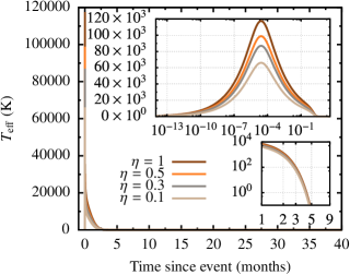
Figure 4.— Time evolution of $T_{\rm eff}$ for various values of $\eta$, following the same order as in Fig. (3). We include two zooms; the top embedded zoom shows in logarithmic scale in the x-axis the whole range of time, from $10^{-13}$ to $9$ months, and the bottom one in linear scale the last few months, from $1$ to $9$, in logarithmic scale in the y-axis.

Since we are dealing with short wavelengths, we can calculate the peak wavelength $\lambda_{\rm peak}$ of the spectral radiance of the cloud as a function of time using an approximation. This is Wien’s displacement law, which relates the absolute temperature $T$ in $K$ and the peak wavelength as $T=b/\lambda_{\rm peak}$, with $b\sim 2.89\,\times 10^{-3}\,\textrm{m\,K}$ Wien’s displacement constant. In Fig. (5) we show the evolution of $\lambda_{\rm peak}$ in the different regimes of frequencies as a function of time.

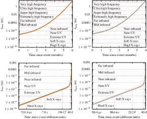
Figure 5.— Top, left panel: Evolution of the peak wavelength $\lambda_{\rm peak}$ of the spectral radiance for the cloud. We display the approximate ranges of the spectrum which it will cover in time. The color scheme follows that of Fig.(4), meaning that $\eta=1$ is the lower curve and the upper one corresponds to $\eta=0.5$. Top, right panel: Same as the left panel for $\eta=0.3$ (upper curve) and $\eta=0.1$ (lower curve). Bottom, left panel: Same as the top, left one, but for different time intervals. We add vertical lines to delimit the different ranges in $\lambda_{\rm peak}$ in time.

4.2. Kinetic temperature

A different definition of temperature is the conversion of kinetic energy into heat as a result of the impact of the stars. This definition will be useful for the derivation of the sound velocity at the innermost region of the outcome of the collision, which will be derived later.

Assuming an ideal gas, the energy and kinetic temperature of the environment are linked via the usual equation

$$E=\frac{3}{2}\,N\,k\,T_{\rm kin},$$ (45)

with and $k$ the Boltzmann constant, $N=M_{\rm tot}/\mu$, $M_{\rm tot}=2\,M_{\odot}$ is the total mass, $\mu=0.6\,m_{\rm p}=5.05\times 10^{-58}\,M_{\odot}$ the mean molecular mass for fully ionised matter, and $m_{\rm p}$ the mass of the proton. We adopt this value because it corresponds to the radiative zone of a star with a mass similar to the Sun, where hydrogen and helium constitute most of all elements. In the surface, where the temperature drops significantly, this assumption would be wrong.

It follows from Eq. (38) that

$$T_{\rm kin}=1.22\times 10^{9}\,\textrm{K}\left(\frac{E(0)}{10^{51}\,\textrm{ergs}}\right)\left(\frac{\eta}{1}\right)\exp\left[-\frac{1}{8}\left(\frac{t}{1\,\textrm{month}}\right)^{2}\right].$$ (46)

We show the evolution of this last equation in Fig. (6).

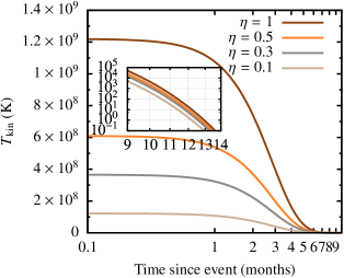
Figure 6.— Evolution of the kinetic temperature as the outcome of the collision with time, given by Eq. (46). We include an embedded zoom of the last few months of evolution and note that in it both axes are in log scale.

4.3. Spectral power

In the previous sections we have estimated the total amount of energy released, as well as the power and the peak wavelength, which can be used as an approximation to understanding the distribution of energy over different bandwidths. In this section we will derive how the power distributes over different ranges of energy. For that, we first have to obtain the distribution of energy in function of time $t$ and frequency $\nu$. Hence, we have to evaluate the following quantity, which we will call the spectral power

$$\frac{dE}{dt\,d\nu}=P(t)\,b\left(T_{\rm eff}(t),\,\nu\right).$$ (47)

In this equation the function $b\left(T_{\rm eff}(t),\,\nu\right)$ is the black body spectrum normalised to $1$ for $T_{\rm eff}(t)$ (i.e. the “observable temperature”) and $\nu$. In terms of integration, $T_{\rm eff}(t)$ can be envisaged as a constant, because we have to integrate in frequencies. I.e. the function corresponds to the spectral radiance of the cloud for frequency $\nu$ at absolute temperature, Planck’s law, but normalised to one,

$$b\left(T_{\rm eff}(t),\,\nu\right)=\frac{B\left(T_{\rm eff}(t),\,\nu\right)}{C\left(T_{\rm eff}(t)\right)}.$$ (48)

Here $B\left(T_{\rm eff}(t),\,\nu\right)$ is

$$B\left(T_{\rm eff}(t),\,\nu\right)=\frac{2h\nu^{3}}{c^{2}}\frac{1}{e^{\,h\nu/(kT)}-1},$$ (49)

with $h$ the Planck constant, $c$ the speed of light, and we are identifying $T\equiv T_{\rm eff}(t)$ for clarity. The integral of this equation over the whole range of $\nu$ does not yield $1$, which is why we need to obtain the normalization factor,

$$C\left(T_{\rm eff}(t)\right)=\int_{\nu=0}^{\nu=\infty}B\left(T_{\rm eff}(t),\,\nu\right)d\nu.$$ (50)

If we change the variable $\alpha=h\nu/(kT)$ so that $d\alpha=hd\nu/(kT)$, we obtain

$$C\left(T_{\rm eff}(t)\right)=2\frac{(kT)^{4}}{c^{2}h^{3}}\int_{0}^{\infty}\frac{\alpha^{3}}{e^{\,\alpha}-1}d{\alpha}.$$ (51)

The integral of Eq. (51) is a special function and a particular case of a Bose–Einstein integral, the Riemann zeta function $\zeta(s)$, a function of a complex variable $s$. The integral is analytical and has the solution

$$\int_{0}^{\infty}\frac{\alpha^{3}}{e^{\,\alpha}-1}d{\alpha}=\zeta(4)\,\Gamma(4),$$ (52)

with $\Gamma(n)$ the Gamma function, $\Gamma(n)=(n-1)!$ if $n$ is a positive integer. Hence, $\zeta(4)\,\Gamma(4)=6\zeta(4)={\pi^{4}}/15$ and so, Eq. (51) becomes

$$C\left(T_{\rm eff}(t)\right)=\frac{2}{15}\frac{\left(Tk\pi\right)^{4}}{c^{2}h^{3}}.$$ (53)

Plugging this result into Eq. (48) and using Eq. (49), we derive that

$$b\,(T,\,\nu)=15\left(\frac{h}{\pi kT}\right)^{4}\frac{\nu^{3}}{e^{\,h\nu/(kT)}-1}.$$ (54)

Therefore, the spectral power of the cloud is

$$\nu\frac{dE}{dt\,d\nu}=\frac{dE}{dt\,d(\ln\nu)}=\frac{15}{\pi^{4}}\,P(t)\frac{\left[h\nu/(kT)\right]^{4}}{e^{\,[h\nu/(kT)]}-1},$$ (55)

where we have multiplied Eq. (47) by $\nu$ to obtain the spectral power in $\ln\nu$, and $P(t)$ is given by Eq. (43). In Fig. (7) we depict the spectral power as a function of $\nu$ for the different values of $\eta$ taken into consideration. With decreasing $\eta$ values, the spectral power is obviously lowered but in the range of observable frequencies, i.e. from $10^{6}\,\textrm{MHz}$, the values achieve relatively high values.

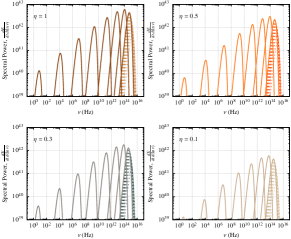
Figure 7.— The spectral power as a function of the frequency $\nu$ for the four different values of the nonlinear parameter $\eta$ taken into consideration. In each of the panels the different curves correspond to different moments in the evolution of the expanding cloud after the stellar collision. From the right (higher values of $\nu$) to the left, we show in dashed lines the first nine tenths of the first month in the evolution, i.e. towards lower frequencies in the first dashed curves there is a time increment of $1/10$ of a month. The first rightmost solid curve corresponds to the spectral power range one month after the event, the second rightmost one, achieving as expected the maximum value, to the second month, etc. We display eight months in the evolution to show the decrease in spectral power, although we note that $10^{6}\,\textrm{MHz}$ corresponds to the lowest frequency of present instruments.

4.4. Photometric colours and AB magnitude

We now display the same information but in a different way. If we define a set a set of passbands (or optical filters), with a known sensitivity to incident radiation, we are in the position of comparing with real data taken from surveys. For that, we first adopt Eq. (55) and remove the factor $\nu$ on the left-hand-side of the equation, so that we are left with this integral to solve

$$\mathcal{C}(t)=\frac{15}{\pi^{4}}\,P(t)\left[h/(kT(t))\right]^{4}\int_{\nu_{\text{min}}}^{\nu_{\text{max}}}\frac{\nu^{3}}{e^{\,[h\nu/(kT(t))]}-1}\,d\nu,$$ (56)

where we have identified $\mathcal{C}\equiv dE/dt$ as the “colour”. Depending on the range of frequencies of interest, we will be looking at different bands. In particular, we define the following ranges for the bands of interest ($\nu$ is given in Hz): U-Band: $\nu_{\text{min}}=7.54\times 10^{14}$, $\nu_{\text{max}}=9.04\times 10^{14}$, B-Band: $\nu_{\text{min}}=6.10\times 10^{14}$, $\nu_{\text{max}}=7.54\times 10^{14}$, G-Band: $\nu_{\text{min}}=5.68\times 10^{14}$, $\nu_{\text{max}}=7.50\times 10^{14}$, V-Band: $\nu_{\text{min}}=5.04\times 10^{14}$, $\nu_{\text{max}}=5.92\times 10^{14}$, R-Band: $\nu_{\text{min}}=4.13\times 10^{14}$, $\nu_{\text{max}}=5.09\times 10^{14}$.

The integral in Eq. (56) is a non-trivial one. However, since the ranges of frequencies that are of our interest are very narrow, what we can do is to approximate the integral by the value of the rectangle delimited by those values. I.e. we simply calculate

$$\frac{dE}{dt}=\frac{15}{\pi^{4}}\,P(t)\frac{\left[h\nu_{\text{avrg}}/(kT(t))\right]^{4}}{e^{\,[h\nu_{\text{avrg}}/(kT(t))]}-1}\ln{\left(\frac{\nu_{\text{max}}}{\nu_{\text{min}}}\right)}.$$ (57)

In this expression, $\nu_{\text{max}}$ and $\nu_{\text{min}}$ are determined by the colour of interest and $\nu_{\text{avrg}}$ is the characteristic frequency associated with that particular band. We can obtain its value by knowing that the length in nm for the various bands is in the U band $l=365$ nm, so that $\nu_{\text{avrg}}=8.21\times 10^{14}$ Hz, in the B band $l=445$ nm, and hence $\nu_{\text{avrg}}=6.74\times 10^{14}$ Hz, in the G band $l=464$, $\nu_{\text{avrg}}=6.46\times 10^{14}$ Hz, in the V band $l=551$ nm, $\nu_{\text{avrg}}=5.44\times 10^{14}$ Hz and in the R band $l=658$ nm, $\nu_{\text{avrg}}=5.56\times 10^{14}$ Hz. The conversion is straightforward, since $\nu_{\text{avrg}}(l)=c/l=3\times 10^{8}/(l\times 10^{-9})$ to obtain Hz. This approximation has an error of about $10\%$ as compared to a numerical integration. In Fig. (8) we show the different evolutions of the photometric indeces as a function of time.

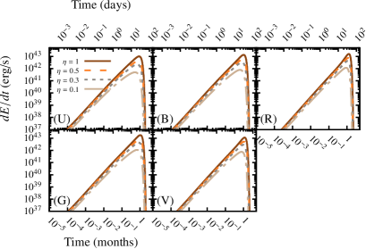
Figure 8.— Photometric indeces U, B, G, V and R as a function of time (in months, lower x-axis and days, upper x-axis) for the different values of the parameter $\eta$.

In order to derive the absolute magnitude (AB magnitude), we remind the reader that it is usually defined as the logarithm of the spectral flux density which defines a zero point value at 3631 Jy. By defining the spectral flux density as $\mathcal{F}$, the AB magnitude can be calculated in cgs units as

$$m_{\text{AB}}=-2.5\log_{10}\mathcal{F}-48.60.$$ (58)

The bandpass AB magnitude spanning across a continuous range of wavelengths is usually defined in such a way that the zero point corresponds to $\mathcal{F}\sim 3631\,\text{Jy}$. Hence,

$$m_{\text{AB}}\approx-2.5\log_{10}\left[{\frac{\int\mathcal{F}{(h\nu)}^{-1}e(\nu)\,\mathrm{d}\nu}{3631\int{(h\nu)}^{-1}e(\nu)\,\mathrm{d}\nu}}\right].$$ (59)

In this expression, $e(\nu)$ is the filter response function and the term ${(h\nu)}^{-1}$ accounts for the photon-counting device.

In Fig. (9) we display the AB magnitude for a typical collision located at a distance of 194.4 Mpc to be able to compare it to the object ZTF19acboexm from the ZTF transient discovery report of Nordin et al. (2019). If this transient had inded its origin in a stellar collision, then the free parameter responsible for the efficiency of the energy conversion should be of about $\eta 0.05$.

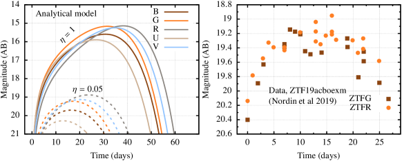
Figure 9.— Left panel: AB magnitude as calculated from the theoretical model at a distance of 194.4 Mpc. We give the extreme values that we have adopted in this work for the free parameter $\eta$, i.e. 1 and also 0.05. Right panel: Zwicky Transient Facility (ZTF) report for 2019-10-07 corresponding to the object ZTF19acboexm by Nordin et al. (2019). The data taken with ZTFG are marked with squares and the data taken with ZTFR with circles. If the transient was the result of a stellar collision, it would seem to correspond to a value of $\eta\lesssim 0.05$.

5. Gravitational waves and multimessenger searches

If we calculate the binding energy of the cores of the stars which initially are on a hyperbolic orbit and compare it to the total kinetic energy of the system as derived in Sec.(3.2), we obtain that the binding energy is of about one order of magnitude below the total kinetic energy. This is a natural consequence of our choice of the problem, since in this work we are focusing on totally disruptive collisional events, which are the most energetic ones.

However, for lower relative velocities, of about $V_{\rm rel}\leq 2500\,\textrm{km\,s}^{-1}$, a fraction of the stellar collisions are such that the inner cores survive the impact and form a temporary binary embedded in a gaseous medium. In this section we will consider a fixed relative velocity of $V_{\rm rel}=1000\,\textrm{km\,s}^{-1}$.

With this new value, when evaluating Eq. (32), we find that the total kinetic energy involved is of $T_{\text{K}}\sim 9.94\times 10^{48}$ ergs, while the binding energy of the two stars is of $E_{\text{bind}}\sim 1.57\times 10^{49}$ ergs (i.e. $\sim 7.6\times 10^{48}$ ergs per star). Therefore, after the collision, one has a gaseous cloud which is expanding very quickly plus two surviving pieces of the stars.

If we assume that $T_{\text{K}}$ is distributed equally among the two colliding stars, then each receives an input of $T_{\text{K}}/2=4.97\times 10^{48}$ ergs. This means that after the collision, there would be a leftover of binding energy per star of approximately 40% the initial binding energy of one star.

Since the core is the densest part of the star, it stands to reason that this 40% represents the core which is surviving. The core of the Sun has a mass of $\sim 0.34\,M_{\odot}$. So all we have after the collision is two cores in a gaseous cloud which is expanding.

The luminosity of a naked core of a Sun-like star radiates at $\sim 4\times 10^{33}$ ergs but the total initial kinetic energy radiated right after the collision is of $\sim 10^{49}$ ergs. We could think that the gaseous cloud will radiate away this energy in such a short timescale that we are left with the two cores which will continue radiating. However, as we will see, the cores will merge before this happens. Therefore we will neglect this extra luminosity of the cores when evaluating the properties of such a “flare” in the following sections.

This kind of collisions is a subfraction of the subset of almost head-on collisions, i.e. for small impact parameters (private communication of Marc Freitag, as published in his PhD thesis, but see Freitag & Benz 2005, as well). In this section we will adopt a representative value of $V_{\rm rel}=10^{3}\,\textrm{km\,s}^{-1}$, i.e. one order of magnitude smaller than before, which is of the order of the velocity dispersion in these environments. We note that the derivation of the absolute rates, however, as derived previously, remain the same, since the assumptions we used still hold for our current choice of $V_{\rm exp}$, even if it is one order of magnitude smaller, as explained in section (2). Nonetheless, Eq. (14) should be multiplied by a fraction number $f_{\rm bin}$ of those simulations which lead to the temporary formation of a core binary. This is the second free parameter of this article (the first is $\eta$, responsible for the non-linearity), which would require dedicated numerical simulations since this information is not contained in Freitag & Benz (2005) or elsewhere to the best of our knowledge.

In this section we consider a low-velocity disruptive collision which firstly leads to a source of electromagnetic radiation. We rederive the quantities and figures of the previous sections for this smaller value of $V_{\rm rel}$. Later, we derive the properties of the binary to then address the evolution of the source of gravitational waves and the prospects for its detection because, as we will see, it could mimic a binary of two supermassive black holes in vacuum, although it should be straightforward to tell them apart.

5.1. Electromagnetic signature of low-velocity collisions

Because we are interested in the electromagnetic precursor of the gravitational wave, we reproduce the previous figures for the effective temperature, energy release, power output and spectral power for the new value of $V_{\rm rel}=10^{3}~{}\textrm{km\,s}^{-1}$, because they change and could be of interest in a search in observational data.

To derive the time evolution of the released energy and power, we must note that Eq. (36) now is $T_{\rm E}\sim 0.52~{}\textrm{yr}\sim 6.2~{}\textrm{months}$ and that $E(0)\sim 10^{49}~{}\textrm{ergs}$. Hence,

$$E(t) \cong 10^{49}\,\textrm{ergs}\left(\frac{E(0)}{10^{49}\,\textrm{ergs}}\right)\left(\frac{\eta}{1}\right)$$

$$\exp\left[-\frac{13}{2000}\left(\frac{t}{1\,\textrm{month}}\right)^{2}\right].$$ (60)

We can see this graphically in Fig. (10). The initial values are significantly lower but the time in which the source is radiating is extended to almost two years in the decay. In Fig. (11) we depict the same as in Fig. (4) but for the new velocity.

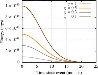
Figure 10.— Same as Fig. (2) but for $V_{\rm exp}=10^{3}~{}\textrm{km\,s}^{-1}$.

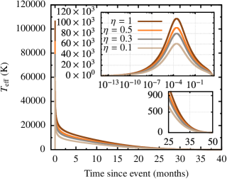
Figure 11.— Same as Fig. (4) but for $V_{\rm exp}=10^{3}~{}\textrm{km\,s}^{-1}$.

In Fig. (12) we display a comparison between the two different cases we are treating, the high-velocity one and the low one. As expected, the temperature peak decreases in the case of low velocity, and lasts longer, so that it is shifted towards later times.

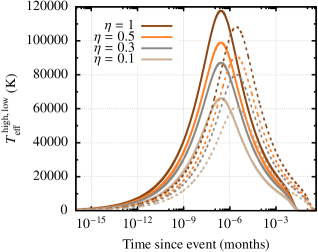
Figure 12.— Comparison of $T_{\rm eff}(\tau)$ for the $V_{\rm exp}=10^{4}~{}\textrm{km\,s}^{-1}$ case (solid lines, $T_{\rm eff}^{\rm high}(\tau)$) and $V_{\rm exp}=10^{3}~{}\textrm{km\,s}^{-1}$ ($T_{\rm eff}^{\rm low}(\tau)$, dashed curves).

As for the emitted power, Eq. (42) becomes

$$P_{\rm norm}\sim 6.32\times 10^{41}\,\textrm{erg\,s}^{-1} \left(\frac{E(0)}{10^{49}\,\textrm{ergs}}\right)\left(\frac{\kappa}{0.04\,\textrm{m}^{2}\textrm{kg}^{-1}}\right)^{-1/2}$$

$$\left(\frac{M}{1\,M_{\odot}}\right)^{-1/2}\left(\frac{V_{\rm exp}}{10^{3}\textrm{km\,s}^{-1}}\right)^{1/2},$$ (61)

and so, the emitted power in the collision of two stars at low velocity is

$$P(t) \sim 6.32\times 10^{41}\textrm{erg\,s}^{-1}\left(\frac{\eta}{1}\right)\left(\frac{t}{1\,\textrm{month}}\right)$$

$$\exp\left[-\frac{13}{2000}\left(\frac{t}{1\,\textrm{month}}\right)^{2}\right]$$

$$\left(\frac{E(0)}{10^{49}\,\textrm{ergs}}\right)\left(\frac{\kappa}{0.04\,\textrm{m}^{2}\textrm{kg}^{-1}}\right)^{-1/2}$$

$$\left(\frac{M}{1\,M_{\odot}}\right)^{-1/2}\left(\frac{V_{\rm exp}}{10^{3}\textrm{km\,s}^{-1}}\right)^{1/2}.$$ (62)

We can see this in Fig. (13). Thanks to this last expression, as explained in the previous section, we can now derive $T_{\rm eff}$ for the low-velocity collision,

$$T_{\rm eff} \cong 1.2\times 10^{6}\,\textrm{K}\left(\frac{\eta}{1}\right)^{1/4}\left(\frac{t}{1\,\textrm{month}}\right)^{1/4}$$

$$\exp\left[-3.25\times 10^{-3}\left(\frac{t}{1\,\textrm{month}}\right)^{2}\right]\left(\frac{E(0)}{10^{49}\,\textrm{ergs}}\right)^{1/4}$$

$$\left(\frac{\kappa}{0.04\,\textrm{m}^{2}\textrm{kg}^{-1}}\right)^{-1/8}\left(\frac{M}{1\,M_{\odot}}\right)^{-1/8}\left(\frac{V_{\rm exp}}{10^{3}\textrm{km\,s}^{-1}}\right)^{1/8}$$

$$\left[1+3777\left(\frac{V_{\rm exp}}{10^{3}\textrm{km\,s}^{-1}}\right)\left(\frac{t}{1\,\textrm{month}}\right)\right]^{-1/2},$$ (63)

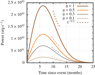
Figure 13.— Same as Fig. (3) but for $V_{\rm exp}=10^{3}~{}\textrm{km\,s}^{-1}$.

Finally, in Fig. (14) we show the corresponding of Fig. (7) but for the lower value of $V_{\rm exp}$. The Eq. (55) needs no modification, but we need to take the correct values for $T_{\rm eff}$ and $P(t)$ into account, i.e. Eq. (63) and Eq. (62) respectively. We note how the spectral power is now concentrated over a much shorter span of frequencies.

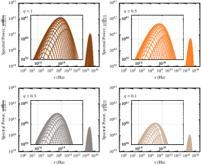
Figure 14.— Same as Fig. (7) but for $V_{\rm exp}=10^{3}~{}\textrm{km\,s}^{-1}$. The solid lines now range from the first month to the 24th and the dashed lines represent the same fraction of time as in Fig. (7). We add a zoom in of each $\eta$.

The kinetic temperature can be estimated as in Eq. (46), but this time the values are accordingly lower,

$$T_{\rm kin}\cong 1.22\times 10^{7}\,\textrm{K}\left(\frac{E(0)}{10^{51}\,\textrm{ergs}}\right)\left(\frac{\eta}{1}\right)$$

$$\exp\left[-\frac{13}{2000}\left(\frac{t}{1\,\textrm{month}}\right)^{2}\right].$$ (64)

In Fig. (15) we depict this evolution. We can see that the values remain higher at later times.

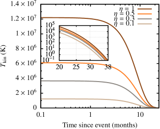
Figure 15.— Same as in Fig. (6) but for $V_{\rm exp}=10^{3}~{}\textrm{km\,s}^{-1}$.

5.2. Point particles in vacuum

Let us now consider the evolution of two point particles in perfect vacuum with the masses of the cores starting at a given semi-major axis and evolving only due to the emission of gravitational radiation. Thanks to the the approximation of non-precessing but shrinking Keplerian ellipses of Peters (1964) we can derive an estimate for the associated timescale for a binary of (point) masses $m_{1}=m_{2}=m_{\rm core}$ and semi-major axis $a$ to shrink only via emission of gravitational radiation,

$$T_{\rm GW}\equiv\frac{a}{|\dot{a}_{\rm GW}|}=\frac{5}{128}\frac{c^{5}\,a^{4}}{G^{3}m_{\rm core}^{3}}F(e)^{-1}.$$ (65)

Normalising to the values we are using,

$$T_{\rm GW}\cong 5\times 10^{8}\textrm{yrs}\left(\frac{m_{\rm core}}{0.34M_{\odot}}\right)^{-3}\left(\frac{a}{R_{\odot}/2}\right)^{4}F(e)^{-1},$$ (66)

where we have chosen the semi-major axis of the cores to be roughly $a\sim d_{\rm min}=R_{\odot}/2$, from Eq. (17). We will however see that this initial choice has little to no impact on the merging time when gas is taken into account.

We have chosen $m_{\rm core}=0.34M_{\odot}$ by assuming that the core radius of the Sun is located at about a distance of $r_{\textrm{core}}\sim 0.2\,R_{\odot}$, following the data in table 3 of Abraham & Iben (1971), and we note that the correction factor $Q$ to multiply this timescale introduced by Zwick et al. (2019) can be neglected, because $Q\sim 1$ in our case. However, as we will see later, the final results are to some extent independent of the choice of initial and final semi-major axes. In the equation we have introduced

$$F(e):=(1-e^{2})^{-7/2}\left(1+\frac{73}{24}e^{2}+\frac{37}{96}e^{4}\right).$$ (67)

For a very eccentric orbit, $e=0.9$, $F(e)^{-1}\sim 2\times 10^{-3}$. I.e. we shorten the timescale by two orders of magnitude. However, even if the eccentricity at binary formation is very large, it circularizes in a very few orbits (see the SPH simulations of Freitag & Benz 2005). We will hence assume $F(e)^{-1}=1$.

Nevertheless, Eq. (66) is nothing but an instantaneous estimation of the (order of magnitude) time for merger due solely to the emission of gravitational radiation. This means that, for a given, fixed, semi-major axis, we obtain a timescale. Nonetheless, the axis shrinks as a function of time, so that $T_{\rm GW}$ will become shorter as well, because it is a function of time. From Eq. (66), and taking into account the original negative sign of Peters (1964), we can derive that

$$\int a^{3}\,da=-\frac{128}{5}\frac{G^{3}\,m_{\rm core}^{3}}{c^{5}}\int dt.$$ (68)

Hence,

$$\frac{a^{4}}{4}=-\frac{128}{5}\frac{G^{3}\,m_{\rm core}^{3}}{c^{5}}\,t+\textrm{constant}.$$ (69)

We can obtain the value of the constant by setting $t=0$, which leads to $\textrm{constant}=a(0)^{4}/4$. Since we have chosen $a(0)\equiv a_{0}=R_{\odot}/2$, we derive that the evolution of the semi-major axis of the binary due only to the emission of gravitational waves is

$$a(t)\cong \Big{[}\frac{1}{16}\left(\frac{a_{0}}{R_{\odot}/2}\right)^{4}$$

$$-4.4\times 10^{-11}\left(\frac{m_{\rm core}}{0.34\,M_{\odot}}\right)^{3}\left(\frac{t}{1\,\textrm{month}}\right)\Big{]}^{1/4}\,R_{\odot}.$$ (70)

In Fig. (16) we show the evolution of Eq. (70).

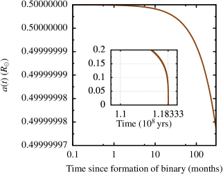
Figure 16.— Evolution of the semi-major axis of the binary since formation, as described by Eq. (70). The embedded panel allows us to see the evolution of the last $0.2\,R_{\odot}$ in units of $10^{8}\,\textrm{yrs}$. The semi-major axis reaches 0 (assuming point-particles) at $t=1.42\times 10^{9}\,\textrm{months}$, as can be derived by setting Eq.(70) to zero.

Replacing Eq. (70) in Eq. (65) leads to

$$T_{\rm GW}(t)\cong \,5\times 10^{8}\,\textrm{yrs}\left(\frac{m_{\rm core}}{0.34\,M_{\odot}}\right)^{-3}\times\Big{[}\left(\frac{a_{0}}{R_{\odot}/2}\right)^{4}$$

$$-7.04\times 10^{-10}\left(\frac{m_{\rm core}}{0.34\,M_{\odot}}\right)^{3}\left(\frac{t}{1\,\textrm{month}}\right)\Big{]}$$ (71)

whose evolution we can see in Fig. (17).

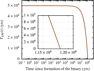
Figure 17.— Evolution of the characteristic timescale $T_{\rm GW}$ as a function of time. The inset allows us to see when it reaches zero. Note that the x-axis in it is in linear scale.

5.3. Cores embedded in a gaseous medium

For a stellar object of mass $m_{\rm obj}$ moving through a homogeneous isothermal gaseous medium of constant density $\rho$ along a straight line with a velocity $V_{\rm obj}$, Ostriker (1999) derives that for a supersonic motion, the drag force provided by dynamical friction as derived by Chandrasekhar (1943) must be modified and is

$$F_{\rm drag}\sim 4\pi\rho\left(\frac{Gm_{\rm obj}}{V_{\rm obj}}\right)^{2}.$$ (72)

Her results have been confirmed numerically by the work of Sánchez-Salcedo & Brandenburg (1999). Hence, for the velocity of one of the two cores to be decreased by one e-folding in the gaseous cloud, the associated timescale is

$$T_{\rm gas}\equiv\frac{V_{\rm core}}{dV_{\rm core}/dt}=\frac{dt}{d\ln{V_{\rm core}}}\cong\frac{m_{\rm core}V_{\rm core}}{F_{\rm drag}},$$ (73)

where $V_{\rm core}$ is the velocity of the core. The last term in the equation is momentum divided by force, which gives an estimate of order of magnitude for the characteristic timescale, the timescale to change $\ln{V_{\rm core}}$ by one dex. We normalise it to the relevant values for this work as

$$T_{\rm gas} \cong 8.4\times 10^{-6}~{}\textrm{yrs}~{}\left(\frac{n}{10^{24}~{}\textrm{cm}^{-3}}\right)^{-1}$$

$$\left(\frac{m_{\rm core}}{0.34M_{\odot}}\right)^{1/2}\left(\frac{a}{R_{\odot}/2}\right)^{-3/2}.$$ (74)

This timescale agrees with the results found by Antoni et al. (2019), in particular their Eq. (37). This is about two orders of magnitude shorter than the orbital period of the binary with the default values in Eq. (74), $P_{\rm orb}=2\pi\sqrt{a^{3}/(2\times G\,m_{\rm core})}$,

$$P_{\rm orb}\sim 1.4\times 10^{-4}\,\textrm{yrs}\left(\frac{a}{R_{\odot}/2}\right)^{3/2}\left(\frac{m_{\rm core}}{0.34\,M_{\odot}}\right)^{-1/2},$$ (75)

which means that the binary would not be able to do one orbit before the cores sink and merge due to the gas. To derive Eq. (74), we have taken as average density that of the Sun, $\rho_{\odot}\sim 1\,\textrm{gr\,cm}^{-3}$, which translates into a numerical density of $10^{24}\textrm{cm}^{-3}$ for the mass of the proton. The amount of gas contained within the orbit can be easily calculated; this is important because, should it be larger than the mass of the cores, then one should use this mass to calculate the orbital velocity. However, for the kind of semi-major axis that we are considering, the mass in gas contained in the orbit of the cores is $M_{\rm gas,\,orb}=\bar{\rho}_{\odot}\times V_{\rm gas,\,orb}\sim 5\times 10^{-3}M_{\odot}<2\times m_{\rm core}$, with $V_{\rm gas,\,orb}$ the volume inside of the orbit and $\bar{\rho}_{\odot}$ the average solar density in the radiative zone, assumed to be $\bar{\rho}_{\odot}=10\,\textrm{g\,cm}^{-3}$. This means that the velocity to take into account to derive Eq. (74) is $V_{\rm core}$, as we have done.

Nonetheless, this derivation of $T_{\rm gas}$ does not take into account the fact that the cores are not moving into a straight line, but they form a binary and hence the density wake around them modifies the drag force (see e.g. Sánchez-Salcedo & Brandenburg 2001; Escala et al. 2004; Kim & Kim 2009). If the semi-major axis is smaller than the Bondi accretion radius,

$$R_{\rm Bondi}=\frac{2\,Gm_{\rm core}}{C_{\rm s}},$$ (76)

with $C_{\rm s}$ the sound speed of the cloud, one needs to correct the gas density around the cores by multiplying $n$ in Eq. (74) by $(R_{\rm Bondi}/a)^{3/2}$ (as realised by Antoni et al. 2019). Since we are assuming almost head-on collisions, we have chosen the semi-major axis for the cores to be of about $R_{\odot}/2$, also motivated by the outcome of the SPH simulations of Freitag & Benz (2005).

Assuming an ideal gas, we can estimate $C_{\rm s}=\sqrt{\gamma_{\text{ad}}\,P/\rho_{\rm g}}$, with $\gamma_{\text{ad}}$ the adiabatic index of the gas, which we assume to be a fully ionized plasma, so that $\gamma_{\text{ad}}=5/3$, and $P$ the pressure, and so $C_{\rm s}=\sqrt{\gamma_{\text{ad}}T(t)k/m}$, with $m=0.6\,m_{\rm p}=1.004\times 10^{-27}\,\textrm{kg}$ and $T(t)$ the temperature of the environment. This temperature is not the effective temperature $T_{\rm eff}(t)$, but the kinetic temperature $T_{\rm kin}(t)$, i.e. the temperature around the cores in the environment in which they are embedded, whose properties we approximate to be those of the radiative zone in the Sun, in terms of fully ionised matter but also of density, as we will see later. Since we are interested in low-velocity collisions, from Eq. (15), we derive that Eq. (74) is

$$T_{\rm gas}\cong 6.4\times 10^{-4}~{}\textrm{yrs} \left(\frac{n}{10^{24}\,\textrm{cm}^{-3}}\right)^{-1}\left(\frac{m_{\rm core}}{0.34\,M_{\odot}}\right)^{-1}$$

$$\left(\frac{C_{\rm s}}{20\,\textrm{kms}^{-1}}\right)^{3},$$ (77)

where we have used the value of $C_{\rm s}$ at $T_{\rm kin}=5\times 10^{2}\,K$ as an illustrative example. However, $T_{\rm kin}$ is a function of time, and hence $C_{\rm s}$ as well, so that plugging in Eq. (64),

$$C_{\rm s}(t)\cong 5.29\times 10^{2}\,\textrm{kms}^{-1}\left(\frac{E(0)}{10^{49}\,\textrm{ergs}}\right)^{1/2}\left(\frac{\eta}{1}\right)^{1/2}$$

$$\exp\left[-\frac{13}{2000}\left(\frac{t}{1\,\textrm{month}}\right)^{2}\right].$$ (78)

In Fig. (19) we depict its evolution with time. It follows the trend of Fig. (11); i.e. because of the temperature quickly drops, so does $C_{\rm s}(t)$ too. We note that this value is in agreement with the results of Vorontsov (1989) (Fig. 2) for the Sun at a radius of about $\sim 1\,R_{\odot}$, with the proviso that the radius is roughly that of the Sun, i.e. at values of $t\sim 0$, which is our departure assumption.

Before we derive the final expression for $T_{\rm gas}(t)$, we note that the density around the cores is not constant; it will decrease with time, since the gaseous cloud is expanding at $V_{\rm exp}$. The SPH simulations of Freitag & Benz (2005) show that when the cores form a binary, the gaseous density around them is of about one order of magnitude lower than the density in the cores.

To derive the initial value of the density around the cores, i.e. at $t=0$, we take the Sun as a reference point. Most of its mass is enclosed in the radiative zone, because the convective zone only represents about $0.3\,R_{\sun}$ and the density in that region is negligible. Following the work of Abraham & Iben (1971), we note that for the mass we have adopted for the cores, $M_{\rm core}=0.34\,M_{\odot}$, the corresponding radius is of $R_{\rm core}\sim 0.2\,R_{\odot}$ and, according to their table 3, the corresponding density in that region is of $\rho\sim 150\,\textrm{g\,cm}^{-3}$. Therefore, we will assume that the density around the cores (corresponding to that of the radiative zone) should be of $\rho_{\rm rad}\sim 15\textrm{g\,cm}^{-3}$ (and hence use the tag “rad”), which corresponds to a numerical density of $n_{\rm rad}\sim 10^{25}\,\textrm{cm}^{-3}$. We therefore only consider a radius of $0.7\,R_{\odot}$, because we are assuming that all mass is in the radiative zone. Taking these considerations into account, plus assuming that the convective zone is fully ionised hydrogen, with the of the proton $m_{p}\sim 1.7\times 10^{-24}$ g, the time evolution of the numerical density around the cores follows the expression

$$n_{\rm rad}(t)\sim 10^{25}\,\textrm{cm}^{-3}\left(\frac{M}{1\,M_{\odot}}\right)$$

$$\left[{\bf\frac{7}{10}}+\frac{19}{5}{\bf\times 10^{3}}\,\left(\frac{V_{\rm exp}}{10^{3}\textrm{km\,s}^{-1}}\right)\left(\frac{t}{1\,\textrm{month}}\right)\right]^{-3}.$$ (79)

We can see this evolution, as well as the evolution of the physical density, in Fig. (18). In a few months the density decreases significantly, so that assuming a constant value would be wrong.

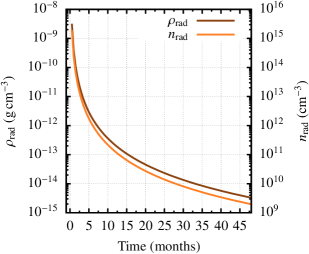
Figure 18.— Evolution of the physical (lower curve) and numerical density (upper curve) of the radiative zone with time, assuming a total mass of $1\,M_{\odot}$ and $V_{\rm exp}=10^{3}\,\textrm{km\,s}^{-1}$. The values corresponding to the physical density, in $\textrm{g\,cm}^{-3}$, are to be read on the left y-axis, and those to the numerical density on the right axis.

Figure 19.— Evolution of the sound speed in the cloud as a function of time. We include a zoom in between months 10 and 30, when it drops to zero. The uppermost curve corresponds to $\eta=1$ and the lowermost to $\eta=0.1$. We add an inset to show the convergence of the models when the sound speed is zero.

We are now in the position of deriving the time dependency of $T_{\rm gas}(t)$ by replacing Eq. (78) and Eq. (79) in Eq. (77),

$$T_{\rm gas}(t) \cong 473.7\,\textrm{yrs}\left(\frac{M}{1\,M_{\odot}}\right)^{-1}\left(\frac{m_{\rm core}}{0.34\,M_{\odot}}\right)^{-1}\left(\frac{\eta}{1}\right)^{3/2}$$

$$\left(\frac{E(0)}{10^{49}\,\textrm{ergs}}\right)^{3}\exp\left[-\frac{39}{2000}\left(\frac{t}{1\,\textrm{month}}\right)^{2}\right]$$

$$\left[1+\frac{19}{5}\left(\frac{V_{\rm exp}}{10^{3}\textrm{km\,s}^{-1}}\right)\left(\frac{t}{1\,\textrm{month}}\right)\right]^{3}$$

In this result, the power of 2 in the exponential for the time stems from the cooling of the cloud via the sound speed, Eq. (77). This quickly decays, as we can see in Fig. (19), and is in power law of 3. The power of 3 in the last term reflects the fact that in our model we assume that the cloud has a volume expanding at a constant rate over time. These are competitive effects responsible for the behaviour of the curve, which we can see see in Fig. (20), where we display Eq.(LABEL:eq.Tgastime). The function initially increases until about $1.5~{}\textrm{yrs}$ from the formation of the binary to then decay. The shape of the curve allows us to estimate when the binary will merge. Since $T_{\rm GW}(t)\gg T_{\rm gas}(t)$, we can ignore the effects of gravitational radiation in the shrinkage of the binary. By evaluating Fig. (20) we can obtain a rough approximation for the binary to merge via gas friction when the elapsed time (i.e. the abscissa, time since the formation of the binary) is larger than $T_{\rm gas}$ and $T_{\rm gas}$ is not increasing in time. We see in the inset of the figure that this requirement is met approximately when $t\sim 2.7~{}\textrm{yrs}$ (for $\eta=1$), which corresponds to $T_{\rm gas}=1~{}\textrm{yr}$. From that point, i.e. $(x,\,y)=(2.7,\,1)\,\text{yrs}$, (i) $t>T_{\rm gas}$ and (ii) $T_{\rm gas}$ is only decreasing in time. Hence, if after $t\sim 2.7~{}\textrm{yrs}$ the binary has not yet merged, it should do so in about $T_{\rm mrg}\sim 1$ year, as an upper limit, as for all other values of $\eta$.

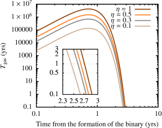
Figure 20.— Evolution of $T_{\rm gas}$ as a function of time, see Eq. (LABEL:eq.Tgastime). The embedded zoom has linear scale in the x-axis ranging from 2.3 years fter the formation of the binary to 3 years. We can see that all of the four models follow a similar behaviour, but the difference between them is not linearly proportional to $\eta$.

To derive a more accurate value for the merger time $T_{\rm mrg}$, we need to derive the evolution of the semi-major axis of the binary due to the drag force of the gas. The differential equation can be derived by taking into account that, for a circular orbit, $V^{2}\propto 1/a$, which means that $\dot{a}/a=-2\dot{V}/V$. Since we have identified in Eq. (73) $V/\dot{V}=T_{\rm gas}$, we have that $\dot{a}/a=-2/T_{\rm gas}$, and hence

$$\int_{R_{\odot}/2}^{a_{\rm mrg}}a^{-1}\,da=-2\int_{0}^{T_{\rm mrg}}T_{\rm gas}^{-1}(t)\,dt,$$ (81)

since we are integrating from the initial semi-major axis $a_{0}=R_{\odot}/2$ to $a_{\rm mrg}$. This final value of the semi-major axis, $a_{\rm mrg}$ is reached when the separation between the cores reaches $R_{\rm core}$. I.e. $a_{\rm mrg}=0.2\,R_{\rm core}$

$$\ln\left(\frac{a_{\rm mrg}=0.2\,R_{\odot}}{a_{0}=R_{\odot}/2}\right)=-2\int_{0}^{T_{\rm mrg}}T_{\rm gas}^{-1}(t)\,dt,$$ (82)

we need to evaluate the right-hand side of the last equation to find the time $t$ for which $a_{\rm mrg}=R_{\rm core}$, although, a priori, from Fig. (20), we already predict that this time is of about 1 yr. Nonetheless, as we already mentioned before, the solution is relatively independent of the initial and final semi-major axis.

In the integral, $T_{\rm gas}$ is given by Eq. (LABEL:eq.Tgastime) and $T_{\rm mrg,\,m}:=T_{\rm mrg}/(\textrm{month})$, and we introduce $\tau:=t/(\textrm{month})$, so that $d\tau=dt/(\textrm{month})$. Hence,

$$\int_{0}^{T_{\rm mrg}}T_{\rm gas}^{-1}(t)\,dt=\frac{1}{\alpha\,\eta}\int_{0}^{T_{\rm mrg,\,m}}e^{\,c\,\tau^{2}}\left(1+b\,\tau\right)^{-3}\,d\tau.$$ (83)

We have introduced $\alpha\equiv 5684.4~{}\textrm{months}$ (see Eq. (LABEL:eq.Tgastime)), $b\equiv{19}/{5}$, and $c\equiv{39}/{2000}$.

The integral given by Eq. (83) can be solved analytically, as we show in Appendix 1. The result is

$$I(x) =\frac{1}{2b}\left[1-\frac{1}{(1+bx)^{2}}\right]+\left(\frac{c}{b^{3}}+\frac{2c^{2}}{b^{5}}\right)e^{\,c/b^{2}}\ln(1+bx)$$

$$-\frac{1}{2bx}\frac{e^{\,cx^{2}}-1}{(1+bx)^{2}}-\frac{cx}{b^{2}}\frac{e^{\,cx^{2}}}{1+bx}$$

$$+\sum_{n=1}^{\infty}\frac{n(2n-1)c^{\,n}}{n!}F_{n}(x).$$ (84)

With

$$F_{n}(x)=\begin{cases}0&n=1\\ \sum_{k=1}^{2n-2}{2n-2\choose k}\frac{(-1)^{\,k}}{k}\left[(1+bx)^{\,k}-1\right]&n>1,\end{cases}$$ (85)

where we have defined $x\equiv T_{\rm mrg}$ for legibility. The solution agrees with standard numerical Gauss-Kronrod quadrature methods to evaluate the value of the integral at different values of $\tau$.

Since

$$\ln\left(\frac{a_{\rm mrg}=0.2}{a_{0}=0.5}\right)=-0.916291=-\frac{2}{\alpha\,\eta}\int_{0}^{T_{\rm mrg,\,m}}I(\tau)\,d\tau,$$ (86)

with $I(\tau)$ the integrand of Eq. (83), and $\ln(a_{\rm mrg}/a_{0})=-\ln(a_{0}/a_{\rm mrg})$, we plot $log(a_{\rm mrg}/a_{0})$ as a function of $\tau$ and look for the value at which

$$0.916291=\frac{2}{\alpha\,\eta}\int_{0}^{T_{\rm mrg,\,m}}I(\tau)\,d\tau,$$ (87)

to find $T_{\rm mrg,\,m}$. In Fig. (21) we show the evolution of the right-hand side of Eq. (83). We can see that from the month 20th the exponential behaviour dominates the evolution of the function and the integral reaches values as high as $10^{70}$. Although mathematically correct, this is a result of the infinite summation of Eq. (84), which is physically only realistic up to the moment at which we consider that the binary forms, i.e. at the value of $\tau$ for which $a_{0}=0.5\,R_{\odot}$, which is $\tau=34.3\,\textrm{months}$. From that moment upwards, the result of the integral is physically meaningless for our purposes. As a consequence of the exponential behaviour, we note that the result is relatively independent of the initial semi-major axis. More precisely, this means that, if we e.g. mutiply by a factor 3 the initial semi-major axis, the result in the x-axis will be larger by a small factor $\epsilon$,

$$\ln\left(\frac{3\times 0.5\,R_{\odot}}{a_{\rm mrg}}\right)=2\times I(T_{\rm mrg}+\epsilon)/(\alpha\,\eta).$$ (88)

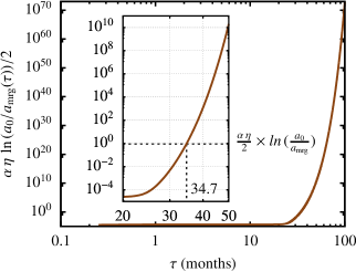
Figure 21.— Evolution of $\alpha\,\eta\,\ln\,(a_{\rm mrg}(\tau)/a_{0})/2$ as a function of $\tau$ (i.e. in months). In the zoom, with a dashed line, we show the values corresponding to $\alpha\eta\times\ln(a_{0}/a_{\rm mrg})/2$. This corresponds to $T_{\rm mrg,\,m}=34.7~{}\textrm{months}$, i.e. $2.892$ yrs, which is off by a value of $0.192$ yr from the value predicted by analysing Fig. (20). We can see that $\tau_{\rm mrg}$ varies very little as a function of $a_{0}$ and $a_{\rm mrg}$, because a big change in distance in the y-axis turns into a small change in the x-axis. This means that the result does not depend (much) on the choice of the initial semi-major axis, which was chosen here to be $R_{\odot}/2$. We display only the value $\eta=1$ because the other values are virtually identical.

5.4. Supermassive black hole mimickers

The drag force acting on to the cores has a direct impact on the observation of the mass of the source in gravitational waves, as shown by Chen & Shen (2019), more precisely on the chirp mass, as introduced by Cutler & Flanagan (1994)

$$M_{\rm chirp}:=\frac{\left(m_{1}m_{2}\right)^{3/5}}{\left(m_{1}+m_{2}\right)^{1/5}},$$ (89)

which reduces in our case to the following trivial expression, since $m_{1}=m_{2}=m_{\rm core}$,

$$M_{\rm chirp}=\frac{1}{2^{1/5}}m_{\rm core}=0.29\,M_{\odot}.$$ (90)

On the detector, however, the evolution of the gravitational wave frequency is affected by the timescale in which the gas shrinks the binary in such a way that the observed chirp mass is not given by Eq. (89) but for

$$M_{\rm chirp,\,obs}(t)=\Big{[}1+\Lambda(t)\Big{]}^{3/5}M_{\rm chirp},$$ (91)

with $\Lambda(t):=T_{\rm GW}(t)/T_{\rm gas}(t)$. This can be seen from Eq. (3) of Chen et al. (2020); Chen & Shen (2019), and is due to the fact that the frequency $f$ and its time derivative $\dot{f}$ now do not evolve solely because of the gravitational radiation (and see also Caputo et al. 2020). In our case, however $T_{\rm gas}$ is a function of time, given by Eq. (LABEL:eq.Tgastime), and $T_{\rm GW}(t)$ is given by Eq. (71). The full expression for $\Lambda(t)$ is

$$\Lambda(t) \cong 10^{6}\left(\frac{M}{1\,M_{\odot}}\right)\left(\frac{m_{\rm core}}{0.34\,M_{\odot}}\right)^{-2}\left(\frac{\eta}{1}\right)^{-3/2}$$

$$\left(\frac{E(0)}{10^{49}\,\textrm{ergs}}\right)^{-3}\exp\left[\frac{39}{2000}\left(\frac{t}{1\,\textrm{month}}\right)^{2}\right]$$

$$\left[1+\frac{19}{5}\left(\frac{V_{\rm exp}}{10^{3}\textrm{km\,s}^{-1}}\right)\left(\frac{t}{1\,\textrm{month}}\right)\right]^{-3}$$

$$\Big{[}\left(\frac{a_{0}}{R_{\odot}/2}\right)^{4}-7.04\times 10^{-10}\left(\frac{m_{\rm core}}{0.34\,M_{\odot}}\right)^{3}\left(\frac{t}{1\,\textrm{month}}\right)\Big{]}$$ (92)

From this and (91), we observe in Fig. (22) the increase of the chirp mass as observed by a gravitational-wave detector such as LIGO/Virgo, the Einstein Telescope or LISA (depending on the observed chirp mass).

The fact that the chirp mass reaches a minimum to then again increase again to higher values is due to the fact that we are taking into account the Bondi radius, Eq. (76), since the cores will be surrounded by a region of overdensity, a “wake” around them. Since the sound speed decreases over time, as we can see in Fig. (19), $R_{\rm Bondi}$ increases. Moreover, the semi-major axis decreases with time, and since we are multiplying Eq. (74) by $(R_{\rm Bondi}/a)^{3/2}$, this translates into an increase over time of the chirp mass.

An advantage of gravitational wave data analysis is that, since the time evolution of the frequency will be very different as compared to the vacuum case, as we show in this article, so that it will become clear that these sources correspond to stellar collisions. This will be the first evidence. The second one is that the merger will be very different to that of a binary of two black holes because there is no event horizon. Last, and also due to the fact that these objects due have a surface, there will be an afterglow.

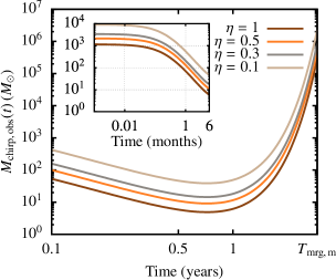
Figure 22.— The observed chirp mass for a binary of two cores of masses $0.34\,M_{\odot}$ each in function of time for the usual four values of $\eta$ (with the highest value in the lowermost curve), as given by Eq. (91). We stop the plot at $T_{\rm mrg,\,m}=2.917\,\textrm{yrs}$, which corresponds to the coalescence time, as derived previously, and include an embedded zoom corresponding to the range $10^{-3}$ months ($1.8$ minutes) to $6$ months.

From the work of Chen & Shen (2019); Chen et al. (2020), the observed distance in gravitational waves due to the same effect has the correction

$$D_{\rm obs}(t)=\big{[}1+\Lambda(t)\big{]}D,$$ (93)

with $D$ the real distance to the source, as derived in Chen et al. (2020). Assuming a vacuum binary of masses $m_{1}=m_{2}=0.34\,M_{\odot}$, semi-major axis $R_{\odot}/2$ and a particular value of the eccentricity, $e=0$, the horizon distance can be estimated to be $D\sim 108\,\textrm{Mpc}$ using the approximant waveform model IMRPhenomPv2 (Khan et al. 2019), a phenomenological model for black-hole binaries with precessing spins, at a flow frequency of $10\,\textrm{Hz}$ with PyCBC (Nitz et al. 2020), an open-source software package designed for use in gravitational-wave astronomy and gravitational-wave data analysis.

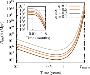
Figure 23.— Evolution of the observed distance to the source, $D_{\rm obs}(t)$ in Mpc as a function of time, following the same nomenclature as in Fig. (22).

In Fig. (23) we can see the evolution of $D_{\rm obs}$ as given by the Eq. (93) with $D\sim 108\,\textrm{Mpc}$. Again, this is a consequence of $\dot{f}$ being different from what you expect in vacuum. As with the chirp mass, the distance will diverge from what is expected in vacuum very quickly. The big missmatch in the chirp mass and the too large distance to the source, but in particular the frequency evolution represent the identifiers of the actual physical origin of the source; namely two colliding stars instead of a binary of two black holes.

5.5. Polarizations in vacuum and in gas

We can relate the polarizations of the waveform amplitude to the chirp mass and the distance to the source in an approximate, Newtonian way as given by the Eqs.(4.30, 4.31, 4.32) of Maggiore (2008), which we reproduce here for convenience.

$$h_{+}(\tau) =\frac{1}{r}\left(\frac{G\,M_{c}}{c^{2}}\right)^{5/4}\left(\frac{5}{c\,\varsigma}\right)^{1/4}\left(\frac{1+\cos^{2}(\iota)}{2}\right)\,\cos\left[\Phi\left(\varsigma\right)\right]$$

$$h_{\times}(\tau) =\frac{1}{r}\left(\frac{G\,M_{c}}{c^{2}}\right)^{5/4}\left(\frac{5}{c\,\varsigma}\right)^{1/4}\cos(\iota)\,\sin\left[\Phi\left(\varsigma\right)\right].$$ (94)

In this equations $\tau$ is our usual definition of $\tau=t/\textrm{month}$, $M_{c}$ is the chirp mass, $\varsigma:=(T_{\rm mrg}-\tau)$, $r$ the distance to the source and $\iota$ is the inclination to the source. Finally, the phase of the gravitational wave $\Phi(\varsigma)$ is the following function,

$$\Phi(\varsigma)=-2\left(\frac{5GM_{c}}{c^{3}}\right)^{-5/8}\varsigma^{5/8}+\Phi_{0},$$ (95)

with $\Phi_{0}$ the value of $\Phi(\varsigma=0)$, and $r$ is the distance to the source, $D$. The value of the constant of Eq. (95) can be derived by setting $\tau=T_{\rm mrg}$. With this we find that in vacuum, the value of $\Phi_{0}$ is

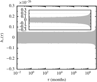
Figure 24.— Plus polarization of the gravitational wave produced by the cores, assuming an inclination of $\iota={45}^{\circ}$. The grey, background curve corresponds to the vacuum waveform. We add a zoom figure showing the interval $10^{9}~{}\textrm{months}$ to $\tau=T_{\rm mrg,\,m}=1.42\times 10^{9}~{}\textrm{months}$. We note that both y-axis need to be multiplies by $10^{-26}$, as displayed in the left, uppermost corner. The small spikes in the waveform are an artifact of the sampling of the plotting program.

$$\Phi_{0}\cong-1.44\times 10^{8}.$$ (96)

Hence, replacing $T_{\rm mrg,\,m}$, we have in vacuum

$$\Phi(\tau)\cong-1.56\times 10^{7}\big{(}35-\tau\big{)}^{5/8}+\Phi_{0},$$ (97)

with $\Lambda(\tau)$ given by Eq. (92) we employ our usual definition of $\tau\equiv t/(\textrm{1~{}month})$.

Taking into account that we have chosen $D=108\,\textrm{Mpc}$ and Eq. (89), and setting $T_{\rm mrg,\,m}=1.42\times 10^{9}~{}\textrm{months}$, Eqs. (94) become

$$h_{+}(\tau) \cong 1.65\times 10^{-25}\Big{[}\big{(}1.42\times 10^{9}-\tau\big{)}\Big{]}^{-1/4}$$

$$\times\left(\frac{1+\cos^{2}(\iota)}{2}\right)\,\cos\left[\Phi\left(\tau\right)\right],$$

$$h_{\times}(\tau) \cong 1.65\times 10^{-25}\Big{[}\big{(}1.42\times 10^{9}-\tau\big{)}\Big{]}^{-1/4}$$

$$\times\cos(\iota)\,\sin\left[\Phi\left(\tau\right)\right],$$ (98)

with $\Phi(\tau)$ given in Eq. (97) and $\Phi_{0}$ in Eq. (96).

In Fig. (24) we display as an example the plus polarization of the Eqs. (98) in vacuum.

In order to derive an expression for the evolution of the polarizations in the case in which we consider the influence of the gas, what we have to do is to analyse the evolution of the semi-major axis of the binary under the influence of the gas, which is given by Eq. (81). In this case, however, we do not integrate up to the merger, i.e. $a=a_{\text{mrg}}$, $t=T_{\text{mrg}}$, but up to some semi-major axis $\hat{a}$ in $R_{\odot}$ and some time $\hat{\tau}$ in units of months. Therefore, we have

$$\hat{a}=\left(\frac{R_{\odot}}{2}\right)\exp\left[-\frac{2}{\alpha\,\eta}\int_{0}^{\hat{\tau}}I(\tau)\,d\tau\right],$$ (99)

with $I(\tau)$ given by Eq. (84). Therefore, for each value of $\hat{\tau}$, we can derive $\hat{a}$ and, with it and Eq. (65), we can obtain what is the time $\varsigma$ that we need to use in the set of Eqs. (94),

$$\varsigma=\frac{5}{128}\frac{c^{5}\,\hat{a}^{4}}{G^{3}m_{\rm core}^{3}}F(e)^{-1}.$$ (100)

I.e. we are deriving the characteristic timescale for an evolution due to gravitational radiation in a case in which the semi-major axis is shrinking at a rate given by the friction with the gas. In Fig. (25) we show the result, which is the counterpart of Fig. (24). We can see that the time has significantly reduced, as well as the width of the oscillations.

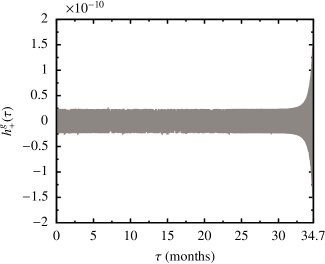
Figure 25.— Plus polarization for the binary embedded in gas. We note that, contrary to Fig. (24), the X-axis is in linear scale.

5.6. Characteristic strain in vacuum and in gas

So as to compare the vacuum case with the one in which the cores are embedded in the gaseous cloud, we will derive the characteristic strain as approximated by Eq. (10.146) of Maggiore (2018),

$$h_{c}(f)=\frac{1}{D}\sqrt{\frac{2}{\pi^{2}}\frac{G}{c^{3}}\frac{dE}{df}},$$ (101)

with $dE/df$ the energy spectrum in the inspiraling phase in the Newtonian approximation, see e.g. Eq. (4.41) of Maggiore (2008),

$$\frac{dE}{df}=\frac{\pi^{2/3}}{3G}\frac{\left(G\,M_{c}\right)^{5/3}}{1+z}\,f^{-1/3}.$$ (102)

We have then

$$h_{c}(f)=\frac{\sqrt{2/3}}{\pi^{2/3}\,c^{3/2}}\frac{\left(G\,M_{c}\right)^{5/6}}{D\sqrt{1+z}}\,f^{-1/6}.$$ (103)

Now, the characteristic strain can be expressed in terms of the amplitude in frequency $A(f)$, the frequency itself $f$ and its time derivative $\dot{f}$ as follows (see Eq. 16.21 of Maggiore 2018),

$$h_{c}(f)=A(f)\frac{f}{\dot{f}^{1/2}},$$ (104)

the only thing we need to do is to take the ratio of the characteristic strain affected by the gas, $h_{c}^{g}(f)$, and that in vacuum, $h_{c}^{v}(f)$. Since the amplitudes and the frequencies are the same, we are left with

$$h_{c}^{\,g}[f(t)] =h_{c}[f(t)]\big{[}\Lambda(t)\big{]}^{-1/2}$$

$$=\frac{\sqrt{2/3}}{\pi^{2/3}\,c^{3/2}}\frac{\left(G\,M_{c}\right)^{5/6}}{D\sqrt{1+z}}\big{[}\Lambda(t)\big{]}^{-1/2}\,f(t)^{-1/6},$$ (105)

with $\Lambda(t)$ given, as usual, by Eq. (92), and $f(t)$ the associated frequency of the source, which is a function of time as well and accordingly needs to be evaluated at the same time as $\Lambda(t)$. This expression, Eq. (105) gives us the instantaneous value of $h_{c}^{g}[f(t)]$ at a given moment $t$.

To derive $f(t)$ we need to take into account two things. First, the driving mechanism in the evolution of the binary, as we have seen previously, is the friction of the binary with the gas, rather than the loss of energy via gravitational radiation, so that in Eq. (105) time derivatives must be done in the context of gas friction. Second, in our derivation of Eq. (81) we used the fact that $\dot{a}/a=-2\dot{V}/V$ and $\dot{a}/a=-2/T_{\rm gas}$. Hence, since the frequency associated to any GW source can be expressed in the Newtonian limit as

$$f=\frac{1}{\pi}\sqrt{\frac{G\,M_{\rm tot}}{a^{3}}},$$ (106)

where $M_{\rm tot}=2\,m_{\rm core}$ and we are omitting the time dependence. The time derivative can be calculated to be

$$\dot{f}_{\rm gas}=-\frac{3}{2\pi}\sqrt{\frac{G\,M_{\rm tot}}{a^{3}}}\frac{\dot{a}_{\rm gas}}{a}.$$ (107)

To derive this expression we have used the chain rule and the fact that what induces a change in the semi-major axis is the gas, so that $da/dt\equiv\dot{a}_{\rm gas}$. I.e. the physical process that induces time changes is the friction with the gas, so that we need to derivate respect to the time the quantities related to it. Hence,

$$\dot{f}_{\rm gas}=3\,\frac{f}{T_{\rm gas}}.$$ (108)

I.e. we need to solve

$$\int f^{-1}\,df=\ln[f(t)]=3\int T_{\rm gas}^{-1}(t^{\prime})\,dt^{\prime}.$$ (109)

As before, in Eq. (83), $T_{\rm gas}$ is given by Eq. (LABEL:eq.Tgastime), $\tau:=t/(\textrm{month})$, so that $d\tau=dt/(\textrm{month})$ and so

$$\ln[f/f_{0}]=3\int T_{\rm gas}^{-1}(t)^{\prime}\,dt^{\prime}=\frac{3}{\alpha\,\eta}\int e^{\,c\,\tau^{2}}\left(1+b\,\tau\right)^{-3}\,d\tau.$$ (110)

With the same values of $\alpha$, $b$ and $c$. In this equation, $f_{0}$ is the initial frequency from which we start to measure the source, and the ratio is $f/f_{0}$ because it is a positive integral.

The result of the previous integral is $3\times I(\tau)$, with $I(\tau)$ given by Eq. (84) and $\tau$ is a moment of time in months before the merger, i.e. at merger $\tau=T_{\rm mrg,\,m}$. Therefore, we have that the integrated characteristic strain from the moment of formation of the binary at a frequency $f_{0}$ and an ulterior given time in months $\tau$ is

$$h_{c}^{\,g}= \frac{\sqrt{6}}{\pi^{2/3}\,c^{3/2}}\frac{\left(G\,M_{c}\right)^{5/6}}{D\sqrt{1+z}}\big{[}\Lambda(\tau)\big{]}^{-1/2}$$

$$\times f_{0}^{\,-1/6}\exp{\left[-\frac{I(\tau)}{2\,\alpha\,\eta}\right]},$$ (111)

with $I(\tau)$ given by Eq. (84) and $\Lambda(\tau)$ by Eq. (92), as usual. As for $f_{0}$, we can derive it from the initial semi-major axis of the binary and the masses of the cores. Since the gravitational-wave frequency is twice the orbital frequency, we have that $f_{0}\cong 4.7\times 10^{-4}\,\textrm{Hz}$.

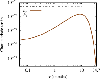
Figure 26.— Evolution of the characteristic strain in vacuum, $h_{\rm c}$, and after the collision, i.e. in a gaseous environment, $h_{\rm c}^{\rm g}$. The two curves correspond to the latter case for two different initial frequencies $f_{0}$, while the former is depicted with a dashed, straight line which does not depend on the initial frequency.

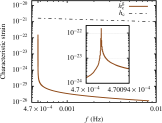
Figure 27.— Same as Fig. (26) but in frequency domain. We include a zoom in for the characteristic strain of the two cores in the gaseous environment between the range of frequencies $f\in[4.7,\,4.70094]\,\times 10^{-4}$ Hz.

We can express the gravitational wave frequency in vacuum of a binary with the same chirp mass as a function of time in months by assuming a Keplerian, circular orbit which shrinks over time via gravitational loss. In the quadrupole approximation and for circular orbits the source orbital frequency $\nu_{s}$ (given via Kepler’s laws) and the gravitational-wave frequency $\nu_{\rm GW}$ are related via $\nu_{\rm GW}=2\,\nu_{s}$. We hence can find from the orbital energy and the fact that $2\pi\,f_{\rm GW}=\nu_{\rm GW}$ that

$$f(t)=\frac{1}{\pi}\left(\frac{G\,M_{c}}{c^{3}}\right)^{-5/8}\left(\frac{5}{256}\frac{1}{\varsigma}\right)^{3/8},$$ (112)

with $\varsigma:=(T_{\rm mrg}-\tau)$. See e.g. Sec. 4.1 of Maggiore (2008) for an explicit derivation of this result. We now substitute this result in Eq. (103) and obtain that

$$h_{c}=\frac{\sqrt{{2}/{3}}\left({5}/{256}\right)^{-3/48}}{\pi^{1/2}c^{29/16}}\frac{\left(GM_{c}\right)^{15/16}}{D\sqrt{1+z}}\left(\frac{1}{\varsigma}\right)^{-3/48}.$$ (113)

If we adopt $D=108\,\textrm{Mpc}$, $z=0$, $M_{c}=0.29\,M_{\odot}$ and introduce $T^{m}_{\rm mrg}:=T_{\rm mrg}/\textrm{month}$ and $\tau$, $h_{c}(t)\cong 4.42\times 10^{-22}\left(T^{m}_{\rm mrg}-\tau\right)^{3/48}$.

In Fig. (26) we can see the differences in the time evolution of the different characteristic strains. The vacuum case corresponds to a straight line as one would expect, since we are working in the inspiral approximation of the quadrupole for circular orbits (as is the case). The cores embedded in the stellar debris, however, evolve in a very different fashion even for the very short timescales related to the problem (of months). At the initial time we see that the strains differ in about three orders of magnitude, as Eq. (105) suggests for the default values given in Eq. (92). In a similar way, in Fig. (27) we depict the frequency evolution of the two strains. Again, in the very short interval of frequencies, the strain in vacuum does not change significantly, while the one corresponding to the gaseous case has a completely different behaviour.

It is interesting to see the propagation in Figs. (26, 27) of the combined effect of the evolution of the speed of sound and the fact that the cloud is expanding over time, as we mentioned in the paragraph following Eq. (LABEL:eq.Tgastime).

We present a sketch of a possible strategy to calculate the mismatch between the vacuum- and the gas sources in Appendix 2.

6. Red giants

So far we have focused on main sequence stars and looked at the high-energy emission and the potential production of an associated gravitational wave source. A particularly interesting kind of star for which the previous analysis can be applied, however, are red giants. This is so because their masses are also of the order of $1\,M_{\odot}$, even if they have much larger radii. When the red giants collide, they will also be a powerful source of high-energy. The presence of a degenerate core at the centre of the star, makes it more appealing from the point of view of gravitational radiation, and when the two degenerate cores collide, this will again turn into a strong source of electromagnetic radiation, which has been envisaged as a possible explanation for Type Ia supernova, such as SN 2006gy (Smith et al. 2007 and see Gal-Yam 2012). We hence would have a precursor electromagnetic signal announcing the gravitational-wave event followed by another posterior, very violent electromagnetic emission.

Contrary to supernovae, red giants come with a different spectrum of masses and radii, and the total mass of the resulting degenerate object would not be constrained by the Chandrasekhar limit. As a consequence, one cannot use them as standard candles. If what is interpreted as Type Ia supernova is mostly the outcome of two colliding red giants, this would have important implications, as we will see.

6.1. Event rate of collisions between red giants

The process of giganterythrotropism, as coined by Peter Eggleton, means that the kind of main sequence stars we have been dealing with in this article will tend to get large and red as they evolve. The main sequence stars we are considering here, of light mass, spend a percentage of their lives in the form of a red giant.

To derive the amount of time spent in the different phases, we refer to the work of Vassiliadis & Wood (1993), in which they estimate that the amount of time spent in the first giant branch (FGB) is of $\sim 3.62\times 10^{9}\textrm{yrs}$, i.e. $24\%$ of the total life of their one-solar mass star of metallicity $Z=0.016$ in their table 1.

Later, the star will reach the asymptotic giant branch (AGB), and during this stage the star’s radius can reach as much as $\sim 215\,R_{\odot}$ (Vassiliadis & Wood 1993). The amount of time spent in the AGB, for a solar-like star is $\tau_{\rm AGB}\sim 2.5\times 10^{7}\textrm{yrs}$ according to Vassiliadis & Wood (1993), which in their model represents $0.17\%$ of the total life of the star

In order to be conservative on the derivation of the rates, this means that the event rates, as derived in the Eq. (14) must be multiplied by a factor of $10^{-2}$ to take this into account, since we need two stars. We pick up a $1\,M_{\odot}$ main sequence star, which in its red-giant phase and a few numerical timesteps before the triple-alpha process has a mass of $M_{\rm RG}=0.953\,M_{\odot}$ and an associated radius of $R_{\rm RG}=25\,R_{\odot}$. We choose these as representative values of our default red giant in the red-giant branch, where the $1\,M_{\odot}$ main-sequence star will stably fuse hydrogen in a shell for about 10% of its entire life.

This has a significant impact on the geometrical cross-section. As we can see in Eq. (14), this leads to an enhancement factor of $\sim 600$ without taking into account the first term enclosed in the square brackets which is, however, basically negligible as compared to the second term in the square brackets as we discussed in that section. We do lose a small factor in terms of mass but, in total, the rates are significantly enhanced. In Fig. (28) we show the equivalent of Fig. (1) but for the collision of two red giants with the above-mentioned properties.

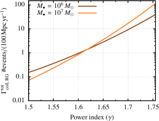
Figure 28.— Same as in Fig. (1) but for red giants of masses $M_{\rm RG}\sim 0.953\,M_{\odot}$ and radii $R_{\rm RG}=25\,R_{\odot}$, taking into account that we have adopted the occupation fraction in phase space for the two giants to be of $f_{\rm RG}=10^{-2}$. This stems from the fact that we are only considering giants in the asymptotic giant branch, where they spend about $0.17\%$ of their life. We do not consider the first giant branch, where they spend up to $24\%$ of their lifetime in order to derive lower-limit quantities.

It is interesting to note that, even though red giants are fully convective, the treatment we have derived in the previous sections regarding the electromagnetic signature still applies to them because the thermodynamics of the gas will not be different from that of the main stars after the collision as soon as the red giants collide, i.e. as soon as they are not in thermodynamical equilibrium.

The compact binary forming in the collision will be surrounded by gas in any case. Even if the impact parameter was exactly zero, there will be gas because the merging time of the compact cores due to the gas drag is much shorter than the timescale in which the gas dissipates.

However, it is interesting to address the formation of the binary which forms because, as we will see in the next section, it is a particular one.

6.2. Structure of the red giants

The nature of the red giant plays a role however in the evolution of the cores in the resulting gaseous cloud that emerges as a result of the collision. This is important for us because we want to understand what source of gravitational radiation the collision will produce after the collision between the two red giants has taken place, with the proviso that the relative speed does not exceed $V_{\rm rel}\leq 2500\,\textrm{km\,s}^{-1}$, as noted in Sec. (5). For this we need to know (i) the average density of the medium in which the cores will be embedded after the collision, (ii) the density of the H-fusing shell around the cores (see ahead in the text), (iii) the masses of the cores and (iv) an estimate of the initial semi-major axes. We will set the mass of the red giant to $M_{\rm RG}=0.953\,M_{\odot}$, which comes from the numerical simulation of a $1\,M_{\odot}$ main-sequence star before reaching the helium flash, where it spends most of its life, and $R_{\rm RG}=25\,R_{\odot}$ (see previous footnote).

In general, a red giant can be envisaged as a self-gravitating, degenerate core embedded in an extended envelope. This is a consequence of the decrease of hydrogen in the inner regions of the star, so that if a main sequence star consumes it, the convective core gives place to an isothermal one. The helium-filled core collapses after reaching a certain maximum (Schönberg & Chandrasekhar 1942) which releases energy that expands the outer layers of the star. However, as proven analytically in the work of Eggleton & Cannon (1991), it is not possible to simply add an envelope fusing H at its base on to a wholly degenerate white dwarf core. One needs to have an (almost) isothermal non-degenerate shell below the fusing shell and above the degenerate core The work of Eggleton & Cannon (1991) proves that the fact that a red giant’s envelope expands, after shell burning is established, is not related to the nature of the envelope, and even of the burning shell, but to the ostensibly small isothermal non-degenerate shell between the degenerate core and the fusing shell.

Since we are interested in the collision and characteristics of the cores when they form a binary and eventually merge via emission of gravitational waves, we need to evaluate the properties of this shell.

We hence consider a red giant as a star with a He-degenerate core, a H-fusing shell around it as the only energy source, transiting through a thin radiative zone to the fully convective, extended envelope. Assuming an ideal gas in the H-fusing shell, the equation of state is

$$P=P_{\rm gas}+P_{\rm rad}=\frac{\Re}{\mu}\rho_{\rm sh}T_{\rm sh}+\frac{a}{3}T_{\rm sh}^{4},$$ (114)

with $\rho_{\rm sh}$ the density in the shell and $T_{\rm sh}$ its temperature, the radiation density constant $a=7.56\times 10^{-15}~{}\textrm{erg}/(\textrm{cm}^{3}\,\textrm{K}^{4})$ and the universal gas constant $\Re=8.31\times 10^{7}~{}\textrm{erg}/\textrm{(K\,g)}$. Usually one introduces $\beta:=P_{\rm gas}/P$, the constant ratio of gas pressure $P_{\rm gas}$ to total pressure $P$, so that $1-\beta=P_{\rm rad}/P$. We can now solve for $\rho_{\rm sh}$,

$$\rho_{\rm sh}=\frac{a\mu}{3\Re}T_{\rm sh}^{3}\frac{\beta}{1-\beta}.$$ (115)

We hence have to derive an estimate for the temperature to obtain the density. For this we follow the derivation of the gradient of temperature with radius as in e.g. (Kippenhahn & Weigert 1991, , their section 5.1.2). We consider the flux of radiative energy $F$ in spherical symmetry in the shell and make an analogy with heat conduction, so that (see Eq. 5.11 of Kippenhahn & Weigert 1991)

$$\frac{dT_{\rm sh}}{dr}=-\frac{\kappa\rho_{\rm sh}\,L}{4\pi acr^{2}T_{\rm sh}^{3}},$$ (116)

where we have absorbed the flux into the luminosity, $L=4\pi r^{2}F$ and $\kappa$ is considered again to be constant, but in this case $\kappa=0.2(1+X)$ for electron scattering. Since $P_{\rm rad}=aT^{4}_{\rm sh}/3$,

$$\frac{dP_{\rm rad}}{dr}=-\frac{1}{4\pi c}\frac{\kappa\rho_{\rm sh}\,L}{r^{2}}.$$ (117)

The equation of hydrostatic equilibrium is

$$\frac{dP}{dr}=-\frac{Gm(r)}{r^{2}}\rho_{\rm sh},$$ (118)

and we approximate $m(r)\sim M_{\rm core}$. Hence

$$dP=\mathcal{C}\,dP_{\rm rad},$$ (119)

with $\mathcal{C}$ constant. We integrate this last equation and take into account that we can neglect the integration constant deep inside the radiative zone, as noted by Paczyński, so that $P/P_{\rm rad}=\mathcal{C}\equiv 4\pi cGM_{\rm core}/(\kappa\,L)=1/(1-\beta)=L_{\rm Edd}/L$. where $L_{\rm Edd}\equiv 4\pi cGM_{\rm core}/\kappa$ is the Eddington luminosity, the maximum luminosity that the source can achieve in hydrodynamical equilibrium (Rybicki & Lightman 1979). If this luminosity was to be exceeded, then radiation pressure would drive the outflow. From Eq. (117) and Eq. (119), we obtain

$$\frac{dT_{\rm sh}}{dr}=-\frac{\kappa L\mu}{16\pi c\Re}\left(\frac{\beta}{1-\beta}\right)\frac{1}{r^{2}}.$$ (120)

Since we have the expression for $(1-\beta)$,

$$\frac{dT_{\rm sh}}{dr}=-\frac{\mu\beta GM_{\rm core}}{4\Re r^{2}}.$$ (121)

We integrate this equation and neglect the constant of integration for the same reasons as we did previously to find

$$T_{\rm sh}=\frac{\mu\beta GM_{\rm core}}{4\Re R_{\rm core}}.$$ (122)

Finally, we obtain that the density can be expressed as

$$\rho_{\rm sh}\cong 6\times 10^{-3}~{}\textrm{g\,cm}^{-3}\frac{\left(\beta\,\mu\right)^{4}}{1-\beta}\left(\frac{M_{\rm core}}{M_{\odot}}\right)^{3}\left(\frac{R_{\rm core}}{R_{\odot}}\right)^{-3},$$ (123)

and we note that we have used the radius of the core $R_{\rm core}$ to normalize the last term, although we are referring to the density in the shell. However, the thickness of the H-fusing shell, $R_{\rm sh}$ extends only a bit farther than the radius of a white dwarf from the center (we use here the letter $R$ for the thickness instead of $T$ because it could be misinterpreted with temperature). This is so because the shell is not (yet) degenerate, but we will also derive the value of $R_{\rm sh}$ later.

We can rewrite Eq. (123) because $\beta$ is constant in the shell, as we have seen previously, so that it can be approximated with a polytrope of index $n=3$, thanks to Eddington’s quartic equation (Eq. 22 of Eddington 1924), which can be written as

$$\frac{1-\beta}{\mu^{4}\beta^{4}}=\frac{a}{3\Re^{4}}\frac{\left(\pi G\right)^{3}c_{1}^{2}}{z_{3}^{6}}M^{2},$$ (124)

with $M$ the total mass of the stellar object, in our case $M=M_{\rm core}$, and $z:=A\,r$ ($A$ a constant) the usual dimensionless variable for the radius introduced to derive the Lane-Emden equation. The value of $z_{3}$ (polytrope of index $n=3$) has to be derived numerically, and is $z_{3}\sim 6.897$ (Chandrasekhar 1939). Finally, the constant $c_{1}$ can be obtained thanks to the relation between central density and average density which one obtains from the Lane-Emden equation, e.g. Eq. (19.20) of Kippenhahn & Weigert (1991), $c_{1}=12.93$. Therefore,

$$\frac{1-\beta}{\mu^{4}\beta^{4}}\cong 3\times 10^{-3}\left(\frac{M_{\rm core}}{M_{\odot}}\right)^{2},$$ (125)

and so, Eq. (123) becomes

$$\rho_{\rm sh}\cong 2\times 10^{4}~{}\textrm{g\,cm}^{-3}\left(\frac{M_{\rm core}}{0.3\,M_{\odot}}\right)\left(\frac{R_{\rm core}}{3\times 10^{-2}\,R_{\odot}}\right)^{-3}.$$ (126)

This result is not unexpected, since the density of a white dwarf ranges between $10^{4}$ and $10^{7}~{}\textrm{g\,cm}^{-3}$, and the H-fusing shell supports pressures very close to that of the degenerate core itself.

We can obtain the mass enclosed between the radius of the white dwarf ($R_{\rm WD}$) and that of the core ($R_{\rm core}$) by integrating Eq. (123),

$$M_{\rm sh}\cong 2\times 10^{-3}\,M_{\odot}\left(\frac{\beta^{4}}{1-\beta}\right)\left(\frac{M_{\rm core}}{M_{\odot}}\right)^{3}\ln\left(\frac{R_{\rm core}}{R_{\rm WD}}\right).$$ (127)

From Eq. (125) and $\mu=0.5$ for pure hydrogen, we have that

$$\frac{1-\beta}{\beta^{4}}\sim 1.7\times 10^{-5}\left(\frac{M_{\rm core}}{0.3M_{\odot}}\right)^{2},$$ (128)

so that Eq. (127) can be rewritten as

$$M_{\rm sh}\cong 3.2\,M_{\odot}\left(\frac{M_{\rm core}}{0.3M_{\odot}}\right)^{3}\ln\left(\frac{R_{\rm core}}{R_{\rm WD}}\right).$$ (129)

The natural logarithm between the two radii and the total mass means that $R_{\rm sh}$ is a minor amount that extends beyond the radius of the degenerate core, approached by a white dwarf in our work.

Therefore, and to first order, we can consider that the properties of the two degenerate objects taking place in the collisions are those of the He core. The numerical code of Eggleton (1971) allows us to obtain the properties of our fiducial model, which is a $1\,M_{\odot}$ red giant. In Fig. (29) we show the evolution of the mass and radius of the He core, while in Fig. (30) we depict the evolution of its density.

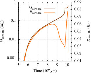
Figure 29.— Evolution of the mass and radius of the He core of a red giant which initially had a $1\,M_{odot}$. The left Y-axis shows the mass of the core in $M_{\odot}$ and the right one the radius in $R_{\odot}$. We can see that, in its evolution, the mass of the core can span three orders of magnitude.

We can see that in particular the mass (and hence the density) significantly vary in the lifetime of the star, while the radius can change by almost one order of magnitude. This means that, when the two degenerate cores form a binary and merge, the properties of the electromagnetic radiation will considerably change depending on which stage of the evolution the red giants are.

In principle we could choose a given mass and radius for the red giants participating in the collision and repeat the whole electromagnetic analysis we have done in the first sections, when we were addressing main sequence stars. This is so because, even if from the point of view of the Eddington standard model of stellar structure a main-sequence star and a red giant are vew different (treated as radiative objects and fully convective, respectively), the gaseous debris after the collision will be similar.

However, because the masses and radii change so much, we decide not to do this exercise just now because we are not aiming at comparing with observational data in this work. It is likely that later we will follow this idea elsewhere.

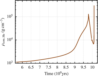
Figure 30.— Same as Fig. (29) but for the density of the core. In its evolution, the different densities can span over two orders of magnitude.

7. Stellar collisions in globular clusters

We have focused so far on galactic nuclei. Covering globular clusters is interesting because the rates are potentially larger due to the smaller relative velocities between the stars participating in the collision which is of the order of the velocity dispersion, as mentioned in the introduction. Indeed, the Table 2 of Baumgardt & Hilker (2018) contains a catalogue of velocity dispersion profiles of 112 Milky Way globular clusters. The average yields $6.57\,\text{km\,s}^{-1}$, so that we will fix the relative velocity of the stars participating in the collision to the average velocity dispersion of $\sigma=7\,\text{km\,s}^{-1}$.

7.1. Rates

While it would be straightforward to repeat the calculations we have presented in Sec. (2) by assuming the presence of an intermediate-mass black hole with a given mass at the centre of the globular cluster, we prefer not to do it. The uncertainty regarding the mass, position (we cannot longer assume it to be fixed at the centre of the system, so that the calculations become more complex) and even existence of such objects would make the rate determination exercise too unconvincing.

However, to motivate this section, the following is a brief summary of the most relevant work that has been done in this context. The problem on the origin of blue stragglers (Maeder 1987; Bailyn 1995; Leonard 1989) is a good choice to try to infer the amount of stellar collisions in globular clusters, since these are very likely the outcome of such collisions.

Leonard (1989) derives a collisional rate of $10^{-8}\,\text{yr}^{-1}$ assuming that a small fraction of main-sequence stars are in primordial binaries. If we take the Milky Way as a reference point, then a galaxy should have of the order of 100 globular clusters, so that the rate is of $10^{-6}\,\text{yr}^{-1}$ per galaxy. This number might be larger, because collisions of binaries are more important Leonard & Fahlman (1991). It is important to note here that the average number of globular clusters correlates with the mass of the central massive black hole (Burkert & Tremaine 2010) in early-type galaxies. In their Fig. (1) we can see that this number can go up by many orders of magnitude depending on the mass of the supermassive black hole. For instance, NGC 4594 has about $2\times 10^{3}$ globular clusters.

A few years later, Sigurdsson & Phinney (1995) carried out a detailed theoretical and numerical study of stellar collisions, and their results suggest a rate that ranges between $10^{-6}$ and $10^{-4}$ main-sequence stellar collisions per year and galaxy (assuming 100 globular clusters). For the arbitrary reference distance that we have adopted of the order of 100 Mpc, we have many clusters of galaxies such as the Virgo Cluster, with about $10^{3}$ galaxies, the Coma Cluster (Abell 1656), also with over $10^{3}$ identified galaxies, and superclusters such as the Laniakea Supercluster (Tully et al. 2014) with about $10^{5}$ galaxies and the CfA2 Great Wall (Geller & Huchra 1989), one of the largest known superstructures, at a mere distance of $\sim 92\,\text{Mpc}$. Regardless of what the rates are, if we took an average of 1000 clusters and the larger rate of $10^{-4}$ of Sigurdsson & Phinney (1995), the number of collisions would be a thousand times larger as compared to 100 clusters per galaxy and the rate of $10^{-6}$. Although the authors did not address red giant collisions, the much larger cross section and the smaller relative velocities in globular clusters are an evidence that their rates must be, as in the case of galactic nuclei, much larger.

7.2. Low relative velocities and impact parameters

Until now we have had the advantage of dealing with collisions that kinematically are very powerful, so that after the collision we have no surviving parts of the star (section 3) or just the core (section 5). However, at a typical relative velocity of $7\,\text{km\,s}^{-1}$, the collision will have a much lower impact on the structure of the stars. We are looking at a different scenario.

On Sec. (2) we mentioned that we neglect gravitational focusing in the case of galactic nuclei. For globular clusters we cannot do this anymore because of the low relative velocity.

The probability of having a collision for a parameter $d_{\text{min}}$, as introduced in Eq. (16) with values ranging between $d_{1}$ and $d_{2}$ is

$$P_{d_{1}\to d_{2}}=\int_{d_{1}}^{d_{2}}\frac{dP}{d\left(d_{\text{min}}\right)}d\left(d_{\text{min}}\right),$$ (130)

where $f(d_{\text{min}})={dP}/{d\left(d_{\text{min}}\right)}$ is the probability density. If we consider a range of $\Delta d:=d_{2}-d_{1}\ll d_{\text{min}}$, then we can approximate the integral by $P_{d_{1}\to d_{2}}\cong f(d_{\text{min}})\Delta d$, as we can see in Fig. (31).

Figure 31.— Probability and probability density as a function of the impact parameter. We depict a generic curve and the two limiting cases we are addressing in this study, namely the case in which $V_{\text{rel}}\ll V_{\text{esc}}$ and $V_{\text{rel}}\gg V_{\text{esc}}$.

When we consider the limit in which $V_{\text{rel}}\gg V_{\text{esc}}$, which corresponds to a galactic nucleus, then $f(d_{\text{min}})\propto d_{\text{min}}$, which is shown in Fig. (31). We can see that in this case, then, the probability of having a collision with $d_{\text{min}}<d$ is proportional to $d^{2}$ (i.e. it is proportional to the “surface”). On the contrary, in the case of a globular cluster, $V_{\text{rel}}\ll V_{\text{esc}}$, so that all impact parameters have the same probability.

What this means is that in a galactic nucleus grazing collisions are more probable than head-on ones, while in a globular cluster a grazing collision and a pure head-on impact have exactly the same probability.

The parameters we used in the previous two sections remain the same but for the relative velocity, which allows us to infer that the kinetic energy deposited on to one star (again, assuming that it is distributed equally) is of $T_{\text{K}}/2\sim 2.43\times 10^{44}\,\text{ergs}$. Hence, after the collision, the star receives an amount of energy equivalent to $3\times 10^{-3}\%$ its initial binding energy. This amount of energy is small enough so that we can investigate the evolution of one of the stars perturbatively.

We will start exploring this situation in its simplest possible form. For that, we consider one collision at a $d_{\text{min}}=\epsilon\left(R_{\text{half},\,1}+R_{\text{half},\,2}\right)$ such that $\epsilon\gtrsim 1$, which leads to contact between the stars after the first close encounter (when they are not bound). The fact that even if $d_{\text{min}}>R_{\text{half},\,1}+R_{\text{half},\,2}$ leads to a potential collision due to the formation of a binary is because of tidal resonances Fabian et al. (1975), because the cross-section is then as large as 1–2 times that of collisions.

The stars we are considering are main-sequence, Sun-like ones. If we consider them (1) to be in hydrostatic equilibrium, (2) to be described by an equation of state of an ideal gas and (3) to be spherical symmetric, then our dynamically stable star reacts on a time given by the hydrostatic timescale

$$\tau_{\mathrm{hydr}}\approx\left(\frac{R_{\odot}^{3}}{GM_{\odot}}\right)^{1/2}\approx\frac{1}{2}(G{\varrho}_{\odot})^{-1/2},$$ (131)

where ${\varrho}$ is the mean density of the star, which we assume to be like our Sun, so that $\tau_{\mathrm{hydr}}\approx 30\,\text{min}$, orders of magnitude shorter than the Kelvin-Helmholtz timescale, which in the case of the Sun is $\tau_{\text{KH}}\sim 1.6\times 10^{7}\,\text{years}$. This timescale is interesting because it can be envisaged as an approximation to the characteristic timescale of a thermal fluctuation, i.e. a thermal adjustment of the star to a perturbation (in the simplistic picture which we are assuming now, since we do not take into account the internal structure). If we are talking about a red giant of mass $1\,M_{\odot}$ and a radius $100\,R_{\odot}$, then $\tau_{\mathrm{hydr}}\approx 18\,\text{days}$.

7.3. Dynamical stability in the adiabatic approach

Let us consider the collision to induce a small perturbation in the star. After the collision, we will assume for simplification that the energy is equally distributed over all the surface of the star, which therefore becomes denser because it is compressed. Since we are assuming this compression to be adiabatic and homologous, the star will abandon its hydrostatic equilibrium. The pressure in one layer of mass of the star can be obtained by evaluating the integral $P=\int^{M}_{m}Gm\,dm/(4\,\pi r^{4})$. Because of homology and adiabaticity, by inspecting both sides of this equation we obtain that

$$\left(\frac{\varrho^{\prime}}{\varrho}\right)^{\gamma_{\text{ad}}}=\left(\frac{R^{\prime}}{R}\right)^{-3\gamma_{\text{ad}}},$$ (132)

where primes represent the values after the collision; i.e. we are dealing with Eq. 25.24 of Kippenhahn & Weigert (1991). This expression tells us that after the collision the star will be dynamically stable in the adiabatic regime if $\gamma_{\text{ad}}>4/3$ because the pressure’s growth is more important than the weight’s increase. Since we are assuming that the stars participating in the collision are Sun-like, we could draw the conclusion that they are stable after the collision since one can approach $\gamma_{\text{ad}}=5/3(>4/3)$. Indeed, in the case of the Sun the layer affected would the convective one, located between $0.7\,R_{\odot}$ and the surface. However, this is a very crude approach in the evaluation of the dynamical stability which needs to be improved because the critical value depends on the simplifications we have adopted in this section (but for the exception of homology, since the threshold for $\gamma_{\text{ad}}$ is the same one for non-homologous scenarios). Moreover, even if the stars are dynamically stable, it is not discarded that they will be instable vibrationally or secularly. We have addressed the dynamical stability because timescale associated is the shortest one.

7.4. Adiabatic pulsations after the collision and considerations about binary formation

Since 1638 we have observed that stars pulsate thanks to the observations of Johannes Phocylides Holwarda of Mira. Arthur Ritter proposed in 1879 that these variations are due to radial pulsations (Gautschy 1997), and Shapley (1914) suggested that the temperature and brightness of Cepheid variables originated in radial pulsations. Later, Eddington (1917), with his piston analogy gave a working frame to describe them. In this valve approximation, the radial pulsation period ${\Pi}_{r}$ can be estimated by calculating the time that a sound wave will need to pass through the star, i.e. ${\Pi}_{r}=2R_{\odot}/C_{\text{s}}$.

We can determine $C_{\text{s}}$ from the pressure $P$ and (mean) density of the star, $C_{\text{s}}^{2}=\gamma_{\text{ad}}\,P/\varrho$, where $\varrho$ is the average density and $\gamma_{\text{ad}}$ is the adiabatic index, the heat capacity ratio or Laplace’s coefficient. It can be envisaged as a measure of the stiffness of the configuration (see e.g. section 38.3 of Kippenhahn & Weigert 1991).

Assuming that $\varrho$ is the actual value of the density througout the whole star and requiring hydrostatic equilibrium, so that ${dP}/{dr}=-{GM\varrho}/{r^{2}}=-G\left({4\pi r^{3}}/{3}\varrho\right){\varrho}/{r^{2}}=-{4G\pi r\varrho^{2}}/{3}$, and requiring that $P=0$ at $r=0$, we derive that $P(r)={2}\pi Gp^{2}\left(R^{2}-r^{2}\right)/3$. Therefore we can obtain that

$${\Pi}_{r} =2\int_{0}^{R}\frac{dr}{\sqrt{{2}\gamma_{\text{ad}}\pi G\rho\left(R^{2}-r^{2}\right)/3}}\approx\sqrt{\frac{3\pi}{2}\left(\gamma_{\text{ad}}G\varrho\right)^{-1}}$$

$$\sim 44.5\,\text{min},$$ (133)

for $\varrho\sim 5.9\,\text{gr\,cm}^{-3}$ after the first collision.

In the adiabatic, spherical approximation, the pulsation is stable and has an associated timescale of about 45 minutes. However, it would be interesting to know if more pulsations can be produced to maintain the rhythm of oscillations typical of the Cepheids. One possible way are further collisions.

7.5. Maintened pulsations

In this section we will quantitatively elucidate possible ways to produce repeated pulsations in a main sequence star that is not in the instability strip through dynamical phenomena, i.e. collisions.

One first idea is that of recurrent collisions due to the formation of a binary after the first impact. The amount of energy loss per collision is $2\times\delta\,E$, with $\delta\,E=T_{\text{K}}\sim 2.44\times 10^{44}\,\text{ergs}$, as we have estimated before. If we just look at the energy, the question whether the two stars will form a binary seems too simple. If the stars are initially on a parabolic orbit, the orbital energy of the system, considered as two mass points (i.e. without taking into account the binding energy of each star) is zero at the beginning (since the relative velocity at infinity is zero, as is the gravitational energy). Any collision -in fact even a close pass without any kind of physical contact which produces tidal effects- will convert kinetic energy into thermal energy and thus leave the stars with negative orbital energy, thus forming a binary.

The real question is how this binary will evolve once it has formed. And this is not a question which can be solved analytically in detail. It is worth to note however that if there is a real contact at the first pericentre passage, a collision, this will make the stars expand, so that further impacts will take place, probably more violent at each successive orbit. The possibility that the binary survives for a long time before the two stars merge is probably low.

These considerations are regarding main-sequence stars, whose envelopes are rather dense. In the case of red giants, it is likely that the the collisions lead to the ejection of the envelope and we are left with a stable binary consisting of the two cores which will then follow the previous scheme: Evolution via gas drag, detection via gravitational radiation and an afterglow when they eventually collide.

This reasoning is for main-sequence stars, whose envelope is quite dense. For giants, perhaps the collisions lead to the ejection of the envelope and we are left with a stable binary consisting of the two cores.

A possible first estime from an energy point of view would be to look at the binding energy of the envelope of the giant; i.e. how much energy leads to an ejection of the envelope and then compare that energy to the orbital energy decrease from the parabolic trajectory to a circular binary formed by the two cores. This would allow us to estimate the semi-major axis of the final binary but this reasoning does not involve the impact parameter at all and is hence simplistic.

The binding gravitational energy of stars in isolation is hence not a useful quantity for studying the formation of binaries. The interesting point has already been addressed: If the relative orbital energy of the two stars is smaller than the sum of the binding energies, it is impossible to destroy both stars completely.

In a globular cluster, it is unlikely for a completely destructive collision to occur, because the relative velocities at infinity are very low. And even if there is enough energy to destroy the stars, we need also a very small impact parameter.

Therefore, for main-sequence stars in a globular cluster, most collisions lead to the formation of a binary star that rapidly merges (in the classical meaning, not the relativistic one). A smaller subset of collisions, those with small impact parameters, produce a direct merger. Very little mass is ejected. But there is a possibility of non-colliding binaries forming due to tidal resonances (Fabian et al. 1975).

Hence, it is difficult to assess analytically the duration and potential periodicity of such pulsations originating from stellar collisions. If they are vibrationally unstable, then we need to input a given amount of energy to maintain the pulses, since the oscillations will damp. The input of energy might (i) come from further collisions with the other star, if they build a binary, (ii) from other stars in the cluster or (iii) internally from the structure of the star, if we have amplitudes increasing in time because the vibrational or thermal instability have excited the star.

Addressing this problem is out of the scope of this paper but it is important to note that pulsating stars are also used as another rung in the standard candle ladder, as pointed out by Henrietta Swan Leavitt (Fernie 1969). Since the implications are potentially important, it would be interesting to investigate the collisional pulsating nature of stars in globular clusters.

This would not be the first time that there is the need to revisit the cosmic ladder argument due to anomalies found in globular clusters. Indeed, if we consider two stars, one of population I (classical Cepheids) and another of population II in the instability strip, they will pulsate due to the $\kappa$ mechanism (see e.g. Kippenhahn & Weigert 1991). Having different masses but same radii because they are located at the same place in the Hertzsprung-Russell diagram. The lighter stars have lower $\varrho$ and, hence, in principle, a longer period than classical Cepheids, even if they have the same luminosity. This is not correct, and the derivation of the correct periods led to Baade to realise that the cosmic distance scale was to be multiplied by a factor of 2 (Baade 1944).

7.6. A scheme to study the injection of energy into the star

Because in globular clusters the relative velocity at infinity is lower than the stellar escape velocity, of the order $500-1000\,\text{km\,s}^{-1}$, the relative velocity at contact is similar to the thermal velocity of stellar matter. Hence, such collisions are only mildly supersonic and entropy is nearly conserved. The entropic variable A defined as $A:=P/\rho^{\gamma_{\text{ad}}}$ (with $P$ the pressure) of a fluid element is subject to increase because of the heat produced during the shock. Nonetheless, because the speed at contact is similar to the speed of sound in the stars participating in the collision, the shocks must have Mach numbers of about unity and hence a weak heating production during the shock. The important point here is that for these reasons, the considered fluid element will have a constant entropic variable during the collisional process, as demonstrated by Lombardi et al. (2002a). This allows us to treat the collision with a semi-analytical approach which is derived by conservation laws of the process. This scheme yields very good results when compared to three-dimensional computer simulations, including shock heating, hydrodynamic mixing, mass ejection, and angular momentum transfer (Lombardi et al. 1996b, 2002a, 2002b, 2003).

In Fig. (32) we show the correlation between the initial and final (i.e. after the collision) entropic index $\Delta A:=A_{\rm fin}-A_{\rm in}$ as a function of the initial pressure of one of the parent stars, $P_{\rm in}$. This finding was already presented in Lombardi et al. (2002b), their Fig. 3, using smoothed-particle hydrodynamics. It is interesting to see that the fluid sorting algorithm gives a result which is very close to what three-dimensional computer simulations yield. We can see that there is a proportion between both quantities such that $\log(\Delta A)\propto\log(1/P_{\rm in})$.

We can use this correlation to our benefit to understand how a collision will add energy to one of the stars after they have gone through an interaction. In particular

$$\log(A_{\rm fin}-A_{\rm in})=b-\log(P_{\rm in}),$$ (134)

so that

$$A=A_{\rm in}+\frac{10^{b}}{\log{P_{\rm in}}}:=A_{\rm in}+\frac{B}{\log{P_{\rm in}}}.$$ (135)

In this equation, $b$ is a constant which contain information about the properties of the collision. For instance, the larger $b$, the more energy will be deposited on to the surface of one of the two stars, and we have defined $B:=10^{\,b}$, which has units of pressure times $A$ (i.e. units of $P^{\,2}/\rho^{\gamma_{\rm ad}}$).

If we consider a weak interaction, we assume that the entropy will be added instantaneously on to the star, and that the density profile will not change. The final pressure is hence

$$P_{\rm fin}=\rho^{\gamma_{\rm ad}}\,A_{\rm fin}=P_{\rm in}+B\,\left(\frac{\rho^{\gamma_{\rm ad}}}{P_{\rm in}}\right),$$ (136)

and therefore the specific internal energy profile is

$$u=\frac{3}{2}\frac{P_{\rm fin}}{\rho}=u_{\rm in}+u_{\rm fin}:=u_{\rm in}+\frac{3}{2}\left(\frac{B}{P_{\rm in}}\right)\rho^{2/3},$$ (137)

because we have adopted $\gamma_{\rm ad}=5/3$. Because the density profile is unchanged, the gravitational potential energy is unchanged as well, which means that only the thermal energy changes, since we are neglecting rotation as a first approach. Therefore, the energy added over the star after the first “hit” is the following integral evaluated over the entire star

$$E_{\rm hit}=\int u_{\rm fin}(m)dm=\int 6\pi\left(\frac{B}{P_{\rm in}(r)}\right)\rho(r)^{5/3}r^{2}dr,$$ (138)

because $dm=\rho\,4\,\pi(r)\,r^{2}\,dr$ in spherical symmetry, which we are assuming.

Eq. (138) allows us to determine $B$ by evaluating the unperturbed parent star. I.e. we solve the equation while setting $B=1$ and then we can choose B to be the desired energy input divided by the result of the equation.

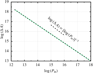
Figure 32.— Difference of the entropic index as a function of the initial pressure of the stars for the following values of the distance of closest approach: $d_{\rm min}/(R_{1}+R_{2})=0,\,0.01,\,0.05,\,0.10,\,0.15,\,0.20,\,0.25,\,0.30,\,0.35,\,0.40,\,0.45,\,0.50,\,0.55,\,0.60i\allowbreak,\,0.65,\,0.70,\,0.75,\,0.80,\,0.85,\,0.90,\,0.95,\,0.99,\,0.999$. We cannot see the different curves because they all follow the same power-law relation, as given with the black, dashed line. In all of the calculations we have assumed $M_{1}=M_{2}=0.8\,M_{\odot}$, a relative velocity at infinity of $7\text{km\,s}^{-1}$ and an initial separation normalized to the sum of the parent star radii of 5.

This scheme allows us to then evaluate the propagation of the energy through the star and the induced pulsations. Unfortunately the analytical calculations require solving the eigenvalue problems of the Sturm-Liouville type to calculate the overtones if we want to consider non-adiabatic, non-radial oscillations, although rotation might help with shearing deformation.

Given that we have seen that any impact parameter has the same probability, we consider that it is not worth extending this article any further than we are already doing. We will therefore study this problem separately in a future publication, either analytically or numerically with the energy injection scheme we have outlined in this section.

8. The cosmic ladder argument

The event rate of colliding red giants and their observational nature is telling us that we might be misinterpreting SNe Ia observations and and be wrong by calling what we observe “standard” candles. Also, their collisions in globular clusters might trigger pulsating stars which are also used as reference points when deriving cosmological scales, as we just pointed out in the last section.

There might be ways to tell them apart in the case of the SNe Ia observations, though. One unique observational signature for WD-WD collisions is the double-peak profile of Cobalt and Iron lines in late-time spectra (also called “nebular spectra”) of SNe Ia Dong et al. (2015). At late times, supernova ejecta become optically thin, so that the line profiles reflect the underlying velocity distributions. Since both, Cobalt and Iron are decay product of Ni56 which is synthesized in the WD-WD merger, the profiles of these Co- and Fe nebular lines show the velocity distribution of Ni56 in the ejecta. The authors studied a sample of some 20 well-observed SNe Ia with nebular spectra, and found in the sample 3 objects showing double peaks and an additional one with a flat-top profile (i.e. departing from a single-peak profile).

This bimodal velocity distribution is a feature of WD-WD mergers (see e.g. the top panels of their Fig. 5). These results are supported by the work of Kushnir et al. (2013), which shows from two-dimensional simulations of WD-WD mergers that the full range of $\sim 0.1-1\,M_{\odot}$ Ni56 can be produced from (exactly head-on) collisions of WDs with masses between $\sim 0.5-1M_{\odot}$. However, other models, such as the one by van Rossum et al. (2016), their Fig. (13), do not predict such double peaks although, as noted by Dong et al. (2015), the observed line profiles depend on the view angle, as well as in other parameters, and their data is not homogeneous, statistically speaking.

Another feature, as shown in Dong et al. (2018) is that for SNe Ia at the very low end of luminosity function, Ni56 ejecta show significantly off-center distribution at about $\sim 1000\,\textrm{km/s}$, which can be explained by WD-WD mergers with significant mass ratios. We note that sub-Chandrasekhar merger models, the delay detonation model, can also produce a large off-center distribution, but not a bi-modal distribution.

It is interesting to note that Wygoda et al. (2019a, b) also explore the WD-WD merger scenario of Kushnir et al. (2013) and they find that the Ni56 column density distribution of the SNe Ia population can be explained in terms of it. Also, Livneh & Katz (2020) find that the key signatures of SNe Ia near the peak, i.e. the diverse distribution of Si II line width distribution, which is usually referred to as the so-called “branch plot”, and widely used to classify SNe Ia population, can be explained by asymmetry in ejecta from WD-WD mergers.

We note that in supernova searches, galactic nuclei are usually left out from the survey because they are complex systems. However, (i) sometimes the whole galaxy is too small in the data to be able to tell apart the nucleus and (ii) as we have mentioned in the introduction, in this work we are focusing on galactic nuclei to evaluate the lower-number case. In globular clusters collisions should happen more frequently due to the lower velocity dispersion, which approximately corresponds to the relative velocity of stars in the system. The lower the relative velocity, the more likely that a gravitational deflection ends up in a collision due to the larger exchange of energy and angular momentum.

9. Conclusions

In this work we have made an analytical study of the electromagnetic- and gravitational radiation implications of stellar collisins between stars in dense stellar systems such as galactic nuclei and globular clusters, whether main-sequence or red giants.

In the case of galactic nuclei, we analyse the remaining gaseous cloud which forms after the impact and its electromagnetic features, while taking into account the ulterior dynamical evolution of the gas, which is expanding and cooling down. In particular, we address the time evolution of the released energy and find that it resembles that of a stellar tidal disruption.

Since we are interested in the observational prospects of detecting this phenomenon, we also describe the time evolution of the effective temperature, the evolution of the peak wavelength of the spectral radiance, as well as the evolution of the kinetic temperature as the outcome of the collision and the spectral power as a function of the frequency.

We find that the electromagnetic traces left by these violent and transient processes strongly resemble over time periods tidal disruptions but also SNe Ia supernovae.

Our complete analysis depends only on two free parameters, one appears in the electromagnetic study and the other one in the gravitational-waves one. In the part dedicated to the electrodynamics, the free parameter is responsible for the non-linearity of the collision, i.e. the transmission of the shocks and hence of the total efficiency conversion of kinetic energy into radiation. The second one, which is relevant for the total rates of gravitational-wave sources, is the number fraction of main-sequence stars whose cores form a binary. We parametrise the solution in terms of the non-linearity parameter and explore four different values. In order to derive this parameter one would need dedicated numerical simulations.

From among the colliding stars, a subgroup of them leads to the formation of a binary consisting of their cores. This subgroup is interesting because it leads to the formation of a binary of two objects that is sufficiently massive and compact to detectably emit gravitational waves.

We find that the friction exerted by the gas accelerates the approach of the surviving cores and brings them closer to eventually merge, with an electromagnetic afterglow such as in the case of binaries of neutron stars merging. Due to the time-varying properties of the gas (which our analytical model takes into account in all calculations), the observed appearance of the gravitational waves is very different from any known source. In particular, two nuclei of very low masses, $0.34\,M_{\odot}$, will be perceived as two black holes of initially slightly above stellar masses, which later increase to become, apparently, two merging supermassive black holes. Something similar happens to the luminance distance, which apparently decreases and then increases very significantly.

As noted in Sec. (5.4), the fact that the frequency evolution is different from the vacuum one, will be the first evidence that these are not black holes emitting gravitational radiation, but a stellar collision. Later, the absence of event horizon will make it obvious and, finally, the electromagnetic afterglow will confirm this. In this sense, the gravitational waves are a perfect tool to identify the nature of the source. We sketch in the second appendix a possible strategy to address the gravitational wave data analysis of the collisions.

We calculate analytical characteristic strains and polarisations of the nuclei in vacuum, as a reference point, and then derive them in the gaseous case, also analytically. The changes are evident and very pronounced, differing by orders of magnitude, although the overall behaviour in the gas case captures, or rather tries to mimic, the behaviour of gravitational radiation emission.

As the gravitational merger time is drastically reduced, electromagnetic and gravitational wave detection go practically hand in hand. This means that the collisions of main-sequence stars and red giants represent two multi-messenger probes that complement each other. This is particularly interesting in the case of red giants, since the core is a degenerate object that will be a more interesting source of gravitational radiation.

In the case of red giants, we calculate the importance of the H-burning shell in the process, as this calculation was not found in the literature, to the best of our knowledge. This is important because this layer around the cores could strongly influence the further evolution of the binary of the two degenerate objects. However, we derive that the role of this shell can be disregarded in this study.

According to our results, these degenerated cores, which can be envisaged as white dwarves, embedded in the host red giants, have a collisional event rate which can be of up to some hundreds of them a year within a volume of $100\,\textrm{Mpc}$. The properties of the collision will strongly vary in function of the mass of the cores and the impact parameter, which depends on the radii of the cores. The properties of these collisions are very similar to SNe Ia. In view of the event rate, this could pose a problem to the interpretations of SNe Ia, which are referred to as “standard candles” following the idea of Henrietta Swan Leavitt (Fernie 1969) as a way to derive cosmological distances following the ladder argument. This is because, as we have just explained, stellar collisions are not standard at all.

Finally, collisions in globular clusters lead to different phenomena, in particular they might lead to stellar pulsation like in the classic problem of the Cepheids. The periodicity of these pulsations is to be investigated because the formation of a binary which is long-lived seems to be unlikely, but collisions arising from other stars can be a way to sustain the pulsations, or vibrational or thermal instabilities triggered in the interior of the star after the first collision. We have shown that their pulsations are stable in the case of the adiabatic, spherical special case, but it is worth to investigate (i) the non-adiabaticity of spherical pulsations and (ii) non-radial oscillations, in both the $\kappa$ and $\epsilon$ mechanisms. We think this is an interesting question because these pulsations are considered to be another rung in the cosmological ladder and, as noted in Sec. (7.4), a misclassification of these has already had an important impact in the past, also in globular clusters. We have not addressed this for the sake of the length of this article, but this is a part of current work and will be presented elsewhere.

Finally, it is worth mentioning that our Galactic Centre is a known region of heightened cosmic ray abundance. Naively, one would have thought that the increase in cosmic ray abundance we observe there would be brought about by a larger abundance of supernovae in this region. However, no such over abundance of supernova is observed in this region. Furthermore, the quiescence level of the supermassive black hole activity in this region casts doubt on an accretion episode being responsible for the cosmic rays. Consequently, a heightened cosmic ray abundance in galactic nuclei appears peculiar, demanding the existence of a regular non-thermal energy source within this region, which seems to be natural to be linked to stellar collisions.

Appendix 1: Analytical solution of the integral associated to $T_{\rm gas}$

The integral 83 to be computed is the following.

$$I(\tau)=\int_{0}^{T_{\rm mrg,\,m}}e^{\,a\,\tau^{2}}\left(1+b\,\tau\right)^{-3}\,d\tau.$$ (139)

We change now the notation, $\tau=t$, $x=T_{\rm mrg,\,m}$, so that

$$I(x)=\int_{0}^{x}\frac{e^{\,ct^{2}}}{(1+bt)^{3}}dt.$$ (140)

Expand the exponential as a power series of $t$.

$$I(x)=\sum_{n=0}^{\infty}\frac{c^{\,n}}{n!}\int_{0}^{x}\frac{t^{2n}}{(1+bt)^{3}}dt.$$ (141)

We now reparametrize the variable $x$ in such a way that the limits of the integral are $0$ and $1$.

$$t=xs,\;\;s=t/x,\;\;dt=xds,$$ (142)

$$I(x)=\sum_{n=0}^{\infty}\frac{c^{\,n}x^{\,2n+1}}{n!}\int_{0}^{1}\frac{s^{\,2n}}{(1+bxs)^{3}}ds=\sum_{n=0}^{\infty}\frac{c^{\,n}x^{\,2n+1}}{n!}I_{n}(x),$$ (143)

where

$$I_{n}(x)=\int_{0}^{1}\frac{s^{\,2n}}{(1+bxs)^{3}}ds.$$ (144)

At this step, we compute the integral $I_{0}$.

$$I_{0}(x) =\int_{0}^{1}\frac{1}{(1+bxs)^{3}}ds=\frac{1}{bx}\int_{0}^{1}\frac{(1+bxs)^{\prime}}{(1+bxs)^{3}}ds$$

$$=-\frac{1}{2bx}\int_{0}^{1}\left[\frac{1}{(1+bxs)^{2}}\right]^{\prime}ds$$

$$=\frac{1}{2bx}\left[1-\frac{1}{(1+bx)^{2}}\right]$$ (145)

We simplify the integral $I_{n}$ for $n\geq 1$ by reducing the power of the denominator, using the method of integration by parts.

$$I_{n}(x) =\int_{0}^{1}\frac{s^{\,2n}}{(1+bxs)^{3}}ds=-\frac{1}{2bx}\int_{0}^{1}s^{\,2n}\left[\frac{1}{(1+bxs)^{2}}\right]^{\prime}ds$$

$$=-\frac{1}{2bx}\left[\frac{s^{\,2n}}{(1+bxs)^{2}}\right]_{s=0}^{s=1}+\frac{n}{bx}\int_{0}^{1}\frac{s^{\,2n-1}}{(1+bxs)^{2}}ds$$

$$=-\frac{1}{2bx}\frac{1}{(1+bx)^{2}}-\frac{n}{bx}\int_{0}^{1}s^{\,2n-1}\left[\frac{1}{1+bxs}\right]^{\prime}ds$$

$$=-\frac{1}{2bx}\frac{1}{(1+bx)^{2}}-\frac{n}{(bx)^{2}}\left[\frac{s^{\,2n-1}}{1+bxs}\right]_{s=0}^{s=1}$$

$$+\frac{n(2n-1)}{(bx)^{2}}\int_{0}^{1}\frac{s^{\,2n-2}}{1+bxs}ds$$

$$=-\frac{1}{2bx}\frac{1}{(1+bx)^{2}}-\frac{n}{(bx)^{2}}\frac{1}{1+bxs}$$

$$+\frac{n(2n-1)}{(bx)^{2}}\int_{0}^{1}\frac{s^{\,2n-2}}{1+bxs}ds.$$ (146)

So, we have to compute the integral

$$f_{n}(x)=\int_{0}^{1}\frac{s^{\,2n-2}}{1+bxs}ds,\;\;n\geq 1.$$ (147)

1. The first thing to do is to simplify the denominator, by using the reparametrization

   $$z=1+bxs,\;\;dz=bxds,\;\;s=\frac{1}{bx}(z-1),$$ (148)

   which gives us

   $$f_{n}(x)=\frac{1}{(bx)^{2n-1}}\int_{1}^{1+bx}\frac{1}{z}(z-1)^{2n-2}dz.$$ (149)

2. Next, we use the binomial theorem to expand the polynomial inside the integral.

   $$(z-1)^{2n-2} =\sum_{k=0}^{2n-2}{2n-2\choose k}(-1)^{\,k}z^{\,k}$$

   $$=1+\sum_{k=1}^{2n-2}{2n-2\choose k}(-1)^{\,k}z^{\,k}.$$ (150)

3. We substitute and have that

   $$\int_{1}^{1+bx}\frac{1}{z}(z-1)^{\,2n-2}dz=\ln(1+bx)+F_{n}(x),$$ (151)

   where we have introduced the polynomial

   $$F_{n}(x)=\begin{cases}0&n=1\\ \sum_{k=1}^{2n-2}{2n-2\choose k}\frac{(-1)^{\,k}}{k}\left[(1+bx)^{\,k}-1\right]&n>1.\end{cases}$$ (152)

4. The integral $f_{n}$ can be expressed via those functions

   $$f_{n}(x)=\frac{1}{(bx)^{2n-1}}\Big{[}\ln(1+bx)+F_{n}(x)\Big{]}.$$ (153)

We now substitute and have that

$$I_{n}(x) =\frac{n(2n-1)}{(bx)^{2n+1}}\Big{[}\ln(1+bx)+F_{n}(x)\Big{]}$$

$$-\frac{1}{2bx}\frac{1}{(1+bx)^{2}}-\frac{n}{(bx)^{2}}\frac{1}{1+bx}$$ (154)

Finally, we combine (4), (6) and (15). Note that all terms apart from the one containing the polynomial $F_{n}$ yield elementary functions.

$$\sum_{n=1}^{\infty} \frac{c^{\,n}x^{\,2n+1}}{n!}\left[-\frac{1}{2bx}\frac{1}{(1+bx)^{2}}\right]$$

$$=-\frac{1}{2bx}\frac{1}{(1+bx)^{2}}\sum_{n=1}^{\infty}\frac{c^{\,n}x^{\,2n+1}}{n!}$$

$$=-\frac{1}{2bx}\frac{e^{\,cx^{2}}-1}{(1+bx)^{2}},$$ (155)

$$\sum_{n=1}^{\infty} \frac{c^{\,n}x^{\,2n+1}}{n!}\left[-\frac{n}{(bx)^{2}}\frac{1}{1+bx}\right]$$

$$=-\frac{1}{(bx)^{2}}\frac{1}{1+bx}\sum_{n=1}^{\infty}\frac{c^{\,n}x^{\,2n+1}}{(n-1)!}$$

$$=-\frac{1}{(bx)^{2}}\frac{1}{1+bx}\sum_{n=0}^{\infty}\frac{c^{\,n+1}x^{\,2n+3}}{n!}$$

$$=-\frac{cx}{b^{2}}\frac{e^{\,cx^{2}}}{1+bx},$$ (156)

$$\sum_{n=1}^{\infty} \frac{c^{\,n}x^{\,2n+1}}{n!}\frac{n(2n-1)}{(bx)^{2n+1}}$$

$$=\frac{1}{b}\sum_{n=1}^{\infty}\frac{2n-1}{(n-1)!}\left(\frac{c}{b^{2}}\right)^{n}=\frac{1}{b}\sum_{n=0}\frac{2n+1}{n!}\left(\frac{c}{b^{2}}\right)^{n+1}$$

$$=\frac{c}{b^{3}}e^{\,c/b^{3}}+\frac{2c}{b^{3}}\sum_{n=0}^{\infty}\frac{n}{n!}\left(\frac{c}{b^{2}}\right)^{n}$$

$$=\frac{c}{b^{3}}e^{\,c/b^{3}}+\frac{2c}{b^{3}}\sum_{n=1}^{\infty}\frac{n}{n!}\left(\frac{c}{b^{2}}\right)^{n}$$

$$=\frac{c}{b^{3}}e^{\,c/b^{3}}+\frac{2c}{b^{3}}\sum_{n=1}^{\infty}\frac{1}{(n-1)!}\left(\frac{c}{b^{2}}\right)^{n}$$

$$=\left(\frac{c}{b^{3}}+\frac{2c^{2}}{b^{5}}\right)e^{\,c/b^{2}}.$$ (157)

Thus:

$$I(x) =\frac{1}{2b}\left[1-\frac{1}{(1+bx)^{2}}\right]+\left(\frac{c}{b^{3}}+\frac{2c^{2}}{b^{5}}\right)e^{\,c/b^{2}}\ln(1+bx)$$

$$-\frac{1}{2bx}\frac{e^{\,cx^{2}}-1}{(1+bx)^{2}}-\frac{cx}{b^{2}}\frac{e^{\,cx^{2}}}{1+bx}$$

$$+\sum_{n=1}^{\infty}\frac{n(2n-1)c^{\,n}}{n!}F_{n}(x).$$ (158)

Appendix 2: A scheme for the gravitational-wave analysis

When comparing the polarizations in the evolving gaseous cloud and vacuum, because of the big difference in $T_{\rm mrg,\,m}$ and $\Lambda(\tau)$, the two polarizations diverge from the beginning. This leads to a significant mismatch of the waveforms.

The reality is more complex. On the one hand, we have a real, physical source which is producing the gravitational radiation. We will refer to this source from now as the “real” source and will use the subscript “r” for it. On the other hand, detectors will receive data for a source which we describe as the “observed” source for obvious reasons, and use the subscript “o” for it. Finally, in order to extract parameters from the observed source, data analysts will use a theoretical model which assumes that the source is in vacuum. This is our “putative” source, and we will use the subscript “p” for it. The connection between these three different sources is displayed in Fig. (33).

Figure 33.— Scheme to derive the various quantities required to compare the observed source and the putative one.

Appendix 3: Neglection of the constant of integration to derive the density of the H-fusing shell

When trying to define the constants of integration of Eq. (119) and Eq. (121) we came accross the unpublished notes of Bohdan Paczyński, where he explains that

The constant (…) can be calculated from the matching conditions between the radiative zone and the outer convective envelope, and it is very important near the radiative - convective boundary. However, deep inside the radiative zone the other two terms in the equation (…) become much larger than the constant, and (it) may be neglected.

We found this explanation in the notes of Jill Knapp in Princeton, who told us it was not her work and after looking for the origin, she found out that the link to the original notes written by Paczyński was Jeremy Goodman. In his turn, he explained that “He (Bohdan Paczyński) taught a class in stellar structure to graduate students for many years, which I had the privilege of helping him with in later years.” Unfortunately, Jeremy could not find a published version of this derivation by Paczyński, so that we acknowledge here the origin of what has led us to the neglection of the constant of integration, crucial in defining the analytical expression for the density of the H-fusing shell.

References

- Abraham & Iben (1971) Abraham, Z., & Iben, Icko, J. 1971, ApJ, 170
- Adams et al. (2004) Adams, T., Davies, M. B., & Sills, A. 2004, MNRAS, 348
- Amaro-Seoane (2019) Amaro-Seoane, P. 2019, Phys.Rev.D., 99, 123025
- Amaro-Seoane et al. (2004) Amaro-Seoane, P., Freitag, M., & Spurzem, R. 2004, MNRAS
- Antoni et al. (2019) Antoni, A., MacLeod, M., & Ramirez-Ruiz, E. 2019, ApJ, 884, 22
- Baade (1944) Baade, W. 1944, ApJ, 100
- Bahcall & Wolf (1976) Bahcall, J. N., & Wolf, R. A. 1976, ApJ, 209
- Bailey & Davies (1999a) Bailey, V. C., & Davies, M. B. 1999a, MNRAS, 308, 257
- Bailey & Davies (1999b) ——. 1999b, MNRAS, 308, 257
- Bailyn (1995) Bailyn, C. D. 1995, ARA&A, 33
- Baumgardt et al. (2018) Baumgardt, H., Amaro-Seoane, P., & Schödel, R. 2018, A&A, 609, A28
- Baumgardt & Hilker (2018) Baumgardt, H., & Hilker, M. 2018, MNRAS, 478, 1520
- Benz & Hills (1987) Benz, W., & Hills, J. G. 1987, ApJ, 323
- Benz & Hills (1992) ——. 1992, ApJ, 389
- Binney & Tremaine (2008) Binney, J., & Tremaine, S. 2008, Galactic Dynamics: Second Edition, ed. J. Binney & S. Tremaine (Princeton University Press)
- Burkert & Tremaine (2010) Burkert, A., & Tremaine, S. 2010, ApJ, 720, 516
- Calderón et al. (2020) Calderón, D., Cuadra, J., Schartmann, M., Burkert, A., Prieto, J., & Russell, C. M. P. 2020, MNRAS
- Caputo et al. (2020) Caputo, A., Sberna, L., Toubiana, A., Babak, S., Barausse, E., Marsat, S., & Pani, P. 2020, ApJ, 892, 90
- Chandrasekhar (1939) Chandrasekhar, S. 1939, Dover Publications Inc.
- Chandrasekhar (1942) ——. 1942, Physical Sciences Data
- Chandrasekhar (1943) ——. 1943, ApJ, 97
- Chen & Shen (2019) Chen, X., & Shen, Z.-F. 2019, arXiv e-prints, arXiv:1906.11055
- Chen et al. (2020) Chen, X., Xuan, Z.-Y., & Peng, P. 2020, arXiv e-prints, arXiv:2003.08639
- Cutler & Flanagan (1994) Cutler, C., & Flanagan, É. E. 1994, Ph. Rev. D, 49, 2658
- da Silva (1993) da Silva, L. A. L. 1993, Astrophysics and Space Science, 202
- Dale et al. (2009) Dale, J. E., Davies, M. B., Church, R. P., & Freitag, M. 2009, MNRAS, 393, 1016
- David et al. (1987a) David, L. P., Durisen, R. H., & Cohn, H. N. 1987a, ApJ, 313
- David et al. (1987b) ——. 1987b, ApJ, 316
- Davies et al. (1991) Davies, M. B., Benz, W., & Hills, J. G. 1991, ApJ, 381
- Davies et al. (1998) Davies, M. B., Blackwell, R., Bailey, V. C., & Sigurdsson, S. 1998, MNRAS, 301
- Davis et al. (2017) Davis, B. L., Graham, A. W., & Seigar, M. S. 2017, MNRAS, 471, 2187
- Dong et al. (2018) Dong, S. et al. 2018, MNRAS, 479, L70
- Dong et al. (2015) Dong, S., Katz, B., Kushnir, D., & Prieto, J. L. 2015, MNRAS, 454, L61
- Eddington (1917) Eddington, A. S. 1917, The Observatory, 40
- Eddington (1924) ——. 1924, MNRAS, 84
- Eggleton (1971) Eggleton, P. P. 1971, MNRAS, 151
- Eggleton & Cannon (1991) Eggleton, P. P., & Cannon, R. C. 1991, ApJ, 383
- Escala et al. (2004) Escala, A., Larson, R. B., Coppi, P. S., & Mardones, D. 2004, ApJ, 607, 765
- Fabian et al. (1975) Fabian, A. C., Pringle, J. E., & Rees, M. J. 1975, MNRAS, 172
- Fernie (1969) Fernie, J. D. 1969, 81
- Freitag & Benz (2001) Freitag, M., & Benz, W. 2001, A&A, 375
- Freitag & Benz (2005) ——. 2005, MNRAS, 358
- Gal-Yam (2012) Gal-Yam, A. 2012, Science, 337, 927
- Gallego-Cano et al. (2018) Gallego-Cano, E., Schödel, R., Dong, H., Nogueras-Lara, F., Gallego-Calvente, A. T., Amaro-Seoane, P., & Baumgardt, H. 2018, A&A, 609, A26
- Gautschy (1997) Gautschy, A. 1997, Vistas in Astronomy, 41
- Geller & Huchra (1989) Geller, M. J., & Huchra, J. P. 1989, Science, 246
- Kelly & Merloni (2012) Kelly, B. C., & Merloni, A. 2012, Advances in Astronomy, 2012, 970858
- Khan et al. (2019) Khan, S., Chatziioannou, K., Hannam, M., & Ohme, F. 2019, Ph.Rv.D, 100, 024059
- Kim & Kim (2009) Kim, H., & Kim, W.-T. 2009, ApJ, 703, 1278
- Kippenhahn & Weigert (1991) Kippenhahn, R., & Weigert, A. 1991, Springer-Verlag
- Kormendy & Ho (2013) Kormendy, J., & Ho, L. C. 2013, ARA&A, 51, 511
- Kushnir et al. (2013) Kushnir, D., Katz, B., Dong, S., Livne, E., & Fernández, R. 2013, ApJ Lett., 778, L37
- Lai et al. (1993) Lai, D., Rasio, F. A., & Shapiro, S. L. 1993, ApJ, 412
- Leonard (1989) Leonard, P. J. T. 1989, AJ, 98
- Leonard & Fahlman (1991) Leonard, P. J. T., & Fahlman, G. G. 1991, AJ, 102
- Livneh & Katz (2020) Livneh, R., & Katz, B. 2020, MNRAS, 494, 5811
- Lombardi et al. (1995) Lombardi, J. C., J., Rasio, F. A., & Shapiro, S. L. 1995, ApJ Lett., 445
- Lombardi et al. (1996a) ——. 1996a, ApJ, 468
- Lombardi et al. (1996b) Lombardi, James C., J., Rasio, F. A., & Shapiro, S. L. 1996b, ApJ, 468, 797
- Lombardi et al. (2002a) Lombardi, James C., J., Warren, J. S., Rasio, F. A., Sills, A., & Warren, A. R. 2002a, ApJ, 568, 939
- Lombardi et al. (2002b) ——. 2002b, ApJ, 568, 939
- Lombardi et al. (2003) Lombardi, J. C., Thrall, A. P., Deneva, J. S., Fleming, S. W., & Grabowski, P. E. 2003, MNRAS, 345, 762
- Maeder (1987) Maeder, A. 1987, A&A, 178
- Maggiore (2008) Maggiore, M. 2008, Gravitational Waves: Volume 1: Theory and Experiments, Gravitational Waves (OUP Oxford)
- Maggiore (2018) ——. 2018, Gravitational Waves: Volume 2: Astrophysics and Cosmology, Gravitational Waves (Oxford University Press)
- Marchant & Shapiro (1979) Marchant, A. B., & Shapiro, S. L. 1979, ApJ, 234
- Marchant & Shapiro (1980) ——. 1980, ApJ, 239
- Mastrobuono-Battisti et al. (2021) Mastrobuono-Battisti, A., Church, R. P., & Davies, M. B. 2021, MNRAS, 505, 3314
- Mathis (1967) Mathis, J. S. 1967, ApJ, 147
- McConnell et al. (2011) McConnell, N. J., Ma, C.-P., Gebhardt, K., Wright, S. A., Murphy, J. D., Lauer, T. R., Graham, J. R., & Richstone, D. O. 2011, Nat, 480, 215
- Murphy et al. (1991) Murphy, B. W., Cohn, H. N., & Durisen, R. H. 1991, ApJ, 370
- Neumayer et al. (2020) Neumayer, N., Seth, A., & Böker, T. 2020, The Astronomy and Astrophysics Review, 28, 4
- Nitz et al. (2020) Nitz, A. et al. 2020, gwastro/pycbc: PyCBC Release v1.15.4
- Nordin et al. (2019) Nordin, J., Brinnel, V., Giomi, M., Santen, J. V., Gal-Yam, A., Yaron, O., & Schulze, S. 2019, Transient Name Server Discovery Report, 2019-2019
- Ostriker (1999) Ostriker, E. C. 1999, ApJ, 513, 252
- Peebles (1972) Peebles, P. J. E. 1972, ApJ, 178
- Peters (1964) Peters, P. C. 1964, Physical Review, 136
- Preto et al. (2004) Preto, M., Merritt, D., & Spurzem, R. 2004, ApJ Lett., 613
- Rees (1988) Rees, M. J. 1988, Nat, 333
- Różyczka et al. (1989) Różyczka, M., Yorke, H. W., Bodenheimer, P., Müller, E., & Hashimoto, M. 1989, A&A, 208
- Rybicki & Lightman (1979) Rybicki, G. B., & Lightman, A. P. 1979, Radiative processes in astrophysics
- Sánchez-Salcedo & Brandenburg (1999) Sánchez-Salcedo, F. J., & Brandenburg, A. 1999, ApJ Lett., 522
- Sánchez-Salcedo & Brandenburg (2001) ——. 2001, MNRAS, 322, 67
- Sanders (1970) Sanders, R. H. 1970, ApJ, 162
- Schödel et al. (2014) Schödel, R., Feldmeier, A., Neumayer, N., Meyer, L., & Yelda, S. 2014, Classical and Quantum Gravity, 31, 244007
- Schödel et al. (2018) Schödel, R., Gallego-Cano, E., Dong, H., Nogueras-Lara, F., Gallego-Calvente, A. T., Amaro-Seoane, P., & Baumgardt, H. 2018, A&A, 609, A27
- Schönberg & Chandrasekhar (1942) Schönberg, M., & Chandrasekhar, S. 1942, ApJ, 96
- Shapiro & Marchant (1978) Shapiro, S. L., & Marchant, A. B. 1978, ApJ, 225
- Shapiro & Teukolsky (1985) Shapiro, S. L., & Teukolsky, S. A. 1985, ApJ Lett., 292
- Shapley (1914) Shapley, H. 1914, ApJ, 40
- Shara (2002) Shara, M. M. 2002, in Astronomical Society of the Pacific Conference Series, Vol. 263, Stellar Collisions, Mergers and their Consequences, ed. M. M. Shara, 1
- Sigurdsson & Phinney (1995) Sigurdsson, S., & Phinney, E. S. 1995, Astrophysical Journal Supplement, 99, 609
- Smith et al. (2007) Smith, N. et al. 2007, ApJ, 666, 1116
- Spitzer & Saslaw (1966) Spitzer, L., J., & Saslaw, W. C. 1966, ApJ, 143
- Spitzer (1987) Spitzer, L. 1987, Dynamical evolution of globular clusters (Princeton, NJ, Princeton University Press, 1987, 191 p.)
- Trac et al. (2007) Trac, H., Sills, A., & Pen, U.-L. 2007, MNRAS, 377, 997
- Tully et al. (2014) Tully, R. B., Courtois, H., Hoffman, Y., & Pomarède, D. 2014, Nat, 513, 71
- van Rossum et al. (2016) van Rossum, D. R., Kashyap, R., Fisher, R., Wollaeger, R. T., García-Berro, E., Aznar-Siguán, G., Ji, S., & Lorén-Aguilar, P. 2016, ApJ, 827, 128
- Vassiliadis & Wood (1993) Vassiliadis, E., & Wood, P. R. 1993, ApJ, 413
- Vergara et al. (2021) Vergara, M. Z. C., Schleicher, D. R. G., Boekholt, T. C. N., Reinoso, B., Fellhauer, M., Klessen, R. S., & Leigh, N. W. C. 2021, 649, A160, 2104.01451
- Vorontsov (1989) Vorontsov, S. V. 1989, Pisma v Astronomicheskii Zhurnal, 15
- Wu et al. (2020) Wu, S., Everson, R. W., Schneider, F. R. N., Podsiadlowski, P., & Ramirez-Ruiz, E. 2020, ApJ, 901, 44
- Wygoda et al. (2019a) Wygoda, N., Elbaz, Y., & Katz, B. 2019a, MNRAS, 484, 3941
- Wygoda et al. (2019b) ——. 2019b, MNRAS, 484, 3951
- Zwick et al. (2019) Zwick, L., Capelo, P. R., Bortolas, E., Mayer, L., & Amaro-Seoane, P. 2019, arXiv e-prints, arXiv:1911.06024