Contrastive Meta-Learning for
Partially Observable Few-Shot Learning

Abstract

Many contrastive and meta-learning approaches learn representations by identifying common features in multiple views. However, the formalism for these approaches generally assumes features to be shared across views to be captured coherently. We consider the problem of learning a unified representation from partial observations, where useful features may be present in only some of the views. We approach this through a probabilistic formalism enabling views to map to representations with different levels of uncertainty in different components; these views can then be integrated with one another through marginalisation over that uncertainty. Our approach, Partial Observation Experts Modelling (POEM), then enables us to meta-learn consistent representations from partial observations. We evaluate our approach on an adaptation of a comprehensive few-shot learning benchmark, Meta-Dataset, and demonstrate the benefits of POEM over other meta-learning methods at representation learning from partial observations. We further demonstrate the utility of POEM by meta-learning to represent an environment from partial views observed by an agent exploring the environment.

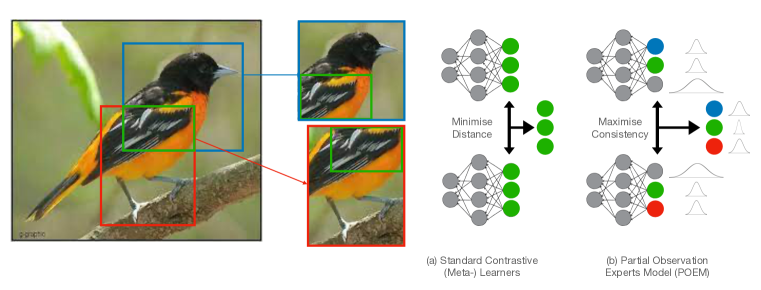
Figure 1: Standard contrastive (meta-) learners minimise a relative distance between representations. This encourages the learning of features that are consistent in all views; in the above example this corresponds to the pattern on the bird’s wing. To better handle partial observability, where features may be disjoint between views, we propose Partial Observation Experts Modelling (POEM). POEM instead maximises consistency between multiple views, by utilising representation uncertainty to learn which features of the entity are captured by a view, and then combining these representations together by weighting features by their uncertainty via a product of experts model (Hinton, 2002).

1 Introduction

Modern contrastive learning methods (Radford et al., 2021; Chen et al., 2020; He et al., 2020; Oord et al., 2019), and embedding-based meta-learning methods such as Prototypical Networks (Snell et al., 2017; Vinyals et al., 2016; Sung et al., 2018; Edwards & Storkey, 2017), learn representations by minimizing a relative distance between representations of related items compared with unrelated items (Ericsson et al., 2021). However, we argue that these approaches may learn to disregard potentially relevant features from views that only inform part of the representation in order to achieve better representational consistency, as demonstrated in Figure 1. We refer to such partially informative views as partial observations. The difficulty with partial observations occurs because distances computed between representations must include contributions from all parts of the representation vector. If the views provided are diverse, and therefore contain partially disjoint features, their representations may appear different to a naive distance metric. For example, two puzzle pieces may contain different information about the whole picture. We call this the problem of integrative representation learning, where we wish to obtain a representation that integrates different but overlapping information from each element of a set.

In this paper, we provide a probabilistic formalism for a few-shot objective that is able to learn to capture representations in partially observable settings. It does so by building on a product of experts (Hinton, 2002) to utilise representation uncertainty: a high variance in a representation component indicates that the given view of the data poorly informs the given component, while low variance indicates it informs it well. Given multiple views of the data, the product of experts component in POEM combines the representations, weighting by the variance, to get a maximally informative and consistent representation from the views.

To comprehensively evaluate our approach, we adapt a large-scale few-shot learning benchmark, Meta-Dataset (Triantafillou et al., 2020), to evaluate representation learning from partial observations. We demonstrate that our approach, Partial Observation Experts Modelling (POEM), is able to outperform standard few-shot baselines on our adapted benchmark, Partially Observed Meta-Dataset (PO-Meta-Dataset), while still matching state-of-the-art on the standard benchmark. Finally, we demonstrate the potential for our approach to be applied to meta-learn representations of environments from the partial views observed by an agent exploring that environment.

The main contributions of this work are: 1) A probabilistic formalism, POEM, that enables representation learning under partial observability; 2) Comprehensive experimental evaluation of POEM on an adaptation of Meta-Dataset designed to evaluate representation learning under partial observability, demonstrating that this approach outperforms standard baselines in this setting while still matching state-of-the-art on the standard fully observed benchmark; 3) A demonstration of a potential application of POEM to meta-learn representations of environments from partial observations.

2 Related Work

2.1 Contrastive Learning

Contrastive learning extracts features that are present in multiple views of a data item, by encouraging representations of related views to be close in an embedding space (Ericsson et al., 2021). In computer vision and natural language applications these views typically consist of different augmentations of data items, which are carefully crafted to preserve semantic features, and thereby act as an inductive bias to encourage the contrastive learner to retain these consistent features (Le-Khac et al., 2020). A challenge in this approach is to prevent representational ‘collapse’, where all views are mapped to the same representation. Standard contrastive approaches such as Contrastive Predictive Coding (Oord et al., 2019), MoCo (He et al., 2020), and SimCLR (Chen et al., 2020) handle this by computing feature space distance measures relative to the distances for negative views – pairs of views that are encouraged to be distinct in the embedding space. In this work we take a similar approach, where the negative views are partial observations of distinct items, but we aim to learn to unify features from differing views, not just retain the consistent features. We learn to learn a contrastive representation from partial views. We note that state-of-the-art representation learning approaches such as CLIP (Radford et al., 2021), which leverage contrastive learning across modalities, also suffer from extracting only a limited subset of features (Fürst et al., 2022) due to using an embedding-based approach (Vinyals et al., 2016) to match image and text representations.

2.2 Embedding-Based Meta-Learning

Embedding-based meta-learners similarly learn representations of classes by extracting features that are consistently present in the data samples (generally referred to as shots in the meta-learning literature) provided for each class, such that the class of new samples can be identified with a similarity measure (Hospedales et al., 2020). These methods generally differ in terms of their approach to combine features, and the distance metric used. Prototypical Networks (Snell et al., 2017) use a Euclidian distance between the query representation and the average over the support representations for a class (referred to as a prototype). Relation Networks (Sung et al., 2018) use the same prototype representation as Prototypical Networks, but use a parameterised relation module to learn to compute the similarity between the query and the prototype rather than using a Euclidian distance. Matching Networks (Vinyals et al., 2016) use a Cosine distance between the query sample and each support sample as a weighting over the support labels, and so perform few-shot classification without unifying the support representations. None of these approaches are designed to unify partially informative support samples. The approach closest to that proposed in this paper is by Edwards & Storkey (2017), where the authors map the different views to a statistic with an associated covariance through a variational approach. However there is no control of the contribution of each view to the variance, and the covariance is spherical, so the approach is also unsuitable for partial observation.

2.3 Optimisation-Based Meta-Learning

The few-shot classification task can also be solved without learning embeddings. One sensible baseline, fine-tuning of a previously pre-trained large model, simply treats each few-shot task as a standard classification problem (Nakamura & Harada, 2019). For each task, one or more additional output layers are added on top of a pre-trained embedding network and trained to predict the classes of the support set (alongside optionally finetuning the embedding network). This can then be utilised to predict the classes of the query set.

Taking this approach a step further, Model-Agnostic Meta-Learning (MAML) (Finn et al., 2017) learns the initialisation of the embedding network, such that it can be rapidly fine-tuned on a new few-shot task. Given the generality of this approach, many variants of this method now exist, such as MAML++, Antoniou et al. (2018), Meta-SGD (Li et al., 2017), CAVIA (Zintgraf et al., 2019) and fo-Proto-MAML (Triantafillou et al., 2020). One variant, LEO (Rusu et al., 2019), performs the meta-optimisation on a latent representation of the embedding parameters, learned using a relational network (Sung et al., 2018). However, none of these variants of this fundamental optimisation based approach to few-shot learning (referred to as ’MAML’ for the remainder of this work) have a mechanism for integrating partial information from the entire support set at inference time, or for comparison with a partial query observation.

2.4 Other Meta-Learning Approaches

Probabilisitic meta-learning methods, such as VERSA (Gordon et al., 2019), DKT (Patacchiola et al., 2020) and Amortised Bayesian Prototype Meta-Learning (Sun et al., 2021), often unify both embedding-based and optimisation based meta-learning by learning to output a posterior distribution that captures uncertainty in predictions, but do not use uncertainty in features to optimally combine support set information. Other recent work, such as DeepEMD (Zhang et al., 2022), has considered the use of attention mechanisms or transformers with image patches (Hiller et al., 2022; Dong et al., 2020), or augmentations (Chen et al., 2021a). However, the purpose of these approaches is to identify informative patches or features within each support example, to improve fine-grained few-shot learning performance or interpretability where relevant features may occupy only a small region of the samples. As far as we know, there are no existing meta-learning methods that aim to integrate partial information from across the support set for comparison with a partially informative query.

2.5 Partial Observability and Product of Experts

Factor analysis is the linear counterpart to modern representation learners, but where partial observability is inherently expressed in the model. The inferential model for the latent space in factor analysis is a product of each of the conditional Gaussian factors. In general, this form of inferential model can be captured as a product of experts (Hinton, 2002). When those experts are Gaussian distributions (Williams et al., 2001), this product of experts is fully tractable. By focusing on the inferential components rather than the linear model, it is possible to generalise factor analysis inference to nonlinear mappings (Tang et al., 2012). However, when only an inferential component is required (as with representation learning), the product of experts can be used more flexibly, as in our approach below.

3 Theoretical Formalism

In this section, we introduce POEM, which incorporates a product of experts model for combining different views with a prior representation, and then uses that representation to classify a query view.

3.1 Product of Expert Prototypes

Let us consider data corresponding to partial observations, or views, of a set of items. In common with most few-shot frameworks, we arrange the data into support sets and query sets. Each support set consists of $M$ data items: $S=\{\mathbf{X}^{m}|{m=1,2,\ldots,M}\}$, where the $m$th item $\mathbf{X}^{m}$ collects $V^{m}$ views, where $V$ may vary with $m$. Let $\mathbf{x}^{m}_{v}$ denote the $v$th view of the $m$th data item, such that $\mathbf{X}^{m}=\{\mathbf{x}^{m}_{1},\mathbf{x}^{m}_{2},\ldots,\mathbf{x}^{m}_{V^{m}}\}$. The items in the support set are sampled randomly from the training dataset. The query point, denoted $\mathbf{x}^{*}$, here consists of a single different view corresponding to one and only one of the $M$ items in the support set (although in general we may consider $N$ query points simultaneously). We cast our representation learning problem as a meta-learning task. We must learn a unified representation derived from the support set that can be compared with a representation of the query view. We want that comparison to enable us to infer which support set item $m=m^{*}$ the query view belongs to.

In this paper we are concerned with partial observability; that is, not every data view will inform the whole representation. So instead of mapping each view to a deterministic point representation, we map each view to a distributional representation where each component is a normalised density that indicates the uncertainty in that component (called a factor). We denote this conditional density $\phi$, and on implementation parameterise the parameters of the distribution $\phi$ with a neural network. We combine the corresponding factors for each view together using a product of experts, which integrates a prior distribution along with the different views such that views with low variance in a component strongly inform that component.

For a given support set, we compute a product of experts distribution for the representation $\mathbf{z}^{m}$:

$$p(\mathbf{z}^{m}|\mathbf{X}^{m})=\frac{p(\mathbf{z}^{m})\prod_{v=1}^{V^{m}}\phi(\mathbf{z}^{m}|\mathbf{x}_{v}^{m})}{\int d\mathbf{z}^{\prime}\ p(\mathbf{z}^{\prime})\prod_{v=1}^{V^{m}}\phi(\mathbf{z}^{\prime}|\mathbf{x}_{v}^{m})},$$ (1)

where $p(\mathbf{z})$ is a prior density over the latent space. Now for a query point with a view that matches other views from e.g. data item $m$, we can use Bayes rule to compute the probability that the query point would be generated from the corresponding representation $\mathbf{z}^{m}$ by

$$p(\mathbf{x}^{*}|\mathbf{z}^{m})=\frac{p(\mathbf{x}^{*})\phi(\mathbf{z}^{m}|\mathbf{x}^{*})}{p(\mathbf{z}^{m})},$$ (2)

where, again, $p(\mathbf{z})=\int d\mathbf{x}\ p(\mathbf{x})\phi(\mathbf{z}|\mathbf{x})$ is the prior.

We put Eq.2 and Eq.1 together and marginalise over $\mathbf{z}^{m}$ to get the marginal predictive distribution

$$p(\mathbf{x}^{*}|\mathbf{X}^{m}) =\int d\mathbf{z}^{m}\ \left(\frac{p(\mathbf{z}^{m})\prod_{v=1}^{V^{m}}\phi(\mathbf{z}^{m}|\mathbf{x}_{v}^{m})}{\int d\mathbf{z}^{\prime}\ p(\mathbf{z}^{\prime})\prod_{v=1}^{V^{m}}\phi(\mathbf{z}^{\prime}|\mathbf{x}_{v}^{m})}\right)\left(\frac{p(\mathbf{x}^{*})\phi(\mathbf{z}^{m}|\mathbf{x}^{*})}{p(\mathbf{z}^{m})}\right)$$ (3)

$$=p(\mathbf{x}^{*})\left(\frac{\int d\mathbf{z}^{m}\ \phi(\mathbf{z}^{m}|\mathbf{x}^{*})\prod_{v=1}^{V^{m}}\phi(\mathbf{z}^{m}|\mathbf{x}_{v}^{m})}{\int d\mathbf{z}^{\prime}\ p(\mathbf{z}^{\prime})\prod_{v=1}^{V^{m}}\phi(\mathbf{z}^{\prime}|\mathbf{x}_{v}^{m})}\right)=p(\mathbf{x}^{*})\frac{\lambda(\mathbf{x}^{*},\mathbf{X}^{m})}{\lambda^{\prime}(\mathbf{X}^{m})}$$ (4)

where

$$\lambda(\mathbf{y},\mathbf{X}) =\int d\mathbf{z}\ \phi(\mathbf{z}|\mathbf{y})\prod_{v=1}^{V}\phi(\mathbf{z}|\mathbf{x}_{v}),\hskip 8.53581pt\mbox{ and}$$ (5)

$$\lambda^{\prime}(\mathbf{X}) =\int d\mathbf{z}\ p(\mathbf{z})\prod_{v=1}^{V}\phi(\mathbf{z}|\mathbf{x}_{v}).$$ (6)

The marginal predictive $p(\mathbf{x}^{*}|\mathbf{X}^{m})$ is used to form the training objective. In our few shot task, we wish to maximize the likelihood for the correct match of query point to support set, accumulated across all support/query selections indexed with $t$ from the dataset. This provides a complete negative log marginal likelihood objective to be minimized, as derived in appendix A.2:

$$\mathcal{L}(\{S_{t}\},\{x_{t}^{*}\})=-\sum_{t}\left[\log\frac{\lambda(\mathbf{x}^{*},\mathbf{X}^{m^{*}})}{\lambda^{\prime}(\mathbf{X}^{m^{*}})}-\log\sum_{m}\frac{\lambda(\mathbf{x}^{*},\mathbf{X}^{m})}{\lambda^{\prime}(\mathbf{X}^{m})}\right]$$ (7)

Full pseudocode for training POEM with this objective is provided in appendix A.3.

3.2 Interpretation of Objective

While the normalised factors $\phi$ can be chosen from any distribution class, we take $\phi$ to be Gaussian with parameterised mean and precision for the remainder of this paper, rendering the integral in Eq. 5 analytic. Approximating the prior $p(\mathbf{z})$ by a Gaussian also renders Eq. 6 analytic. We note that other distributions with analytic products, such as Beta distributions, may also be of interest in certain applications, but we leave an investigation of other distributional forms for $\phi$ to further work.

If the representations from each view for a support point are aligned with each other and the query view (the means of all the Gaussians are similar), they will have a greater overlap and the integral of the resulting product of Gaussians will be larger, leading to a greater value of $\lambda(y,\mathbf{X})$. Furthermore, increasing the precisions for aligned Gaussian components leads to greater $\lambda(y,\mathbf{X})$, while, up to a limit, decreasing the precisions for non-aligned Gaussian components leads to greater $\lambda(y,\mathbf{X})$.

While the numerator in Eq. 4, $\lambda(y,\mathbf{X})$, quantifies the overlap of the support set with the query, the denominator $\lambda^{\prime}(\mathbf{X})$ contrasts this with the overlap of the support set representation with the prior. Together, this factor is enhanced if it is beneficial in overlap terms to replace the prior with the query representation, and reduced if such a replacement is detrimental. A greater consistency between query and combined support set representations intuitively leads to a greater probability that the query belongs to the class of the corresponding support set, effectively extending Prototypical Networks to a probabilistic latent representation space (Snell et al., 2017).

As a result, this objective is a generalisation of a Prototypical Network that allows for (a) learnable weighted averaging over support examples based on their informativeness to a given component; (b) learnable combinations of features from subsets of support examples (via differing relative precisions of components within support representations), and (c) partial comparison of the query sample with the support samples (via differing relative precisions within the query). With all precisions fixed to 1, this approach reproduces Prototypical Networks, neglecting small differences in scaling factors that arise with varying numbers of views. This relationship is derived in Appendix A.4.

4 Experimental Evaluation

There is a lack of established benchmarks specifically targeted at the evaluation of representation learning under partial observability. To design a comprehensive benchmark for few-shot representation learning under partial observability, we leverage Meta-Dataset (Triantafillou et al., 2020), a recently proposed collection of few-shot learning benchmarks. We selected Meta-Dataset as the basis for our adapted benchmark as it consists of diverse datasets involving natural, human-made and text-based visual concepts, with a variety of fine-grained classification tasks that require learning from varying and unbalanced numbers of samples and classes. As a result, our derived benchmark inherits these properties to provide a robust measure of the ability of a learning approach to learn representations from partial observations.

To extend Meta-Dataset to incorporate partial observability, we take multiple views of each sample and divide these views into support and query sets. Our adapted few-shot classification task is to predict which sample a query view comes from, given a selection of support views of that sample, as demonstrated in Figure 2.

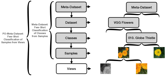
Figure 2: Standard few-shot learning requires the prediction of an image class from a sample. Our adapted task evaluates representation learning under partial observability by instead requiring prediction of the underlying image from partial views. Views are generated with the standard contrastive augmentations, with stronger cropping. We call the resulting benchmark Partially Observable Meta-Dataset (PO-Meta-Dataset).

In keeping with the spirit of Meta-Dataset, we vary the number of ways in the task (now the number of images) from 5 to 25, taken from between 1 to 5 classes. Views are generated by applying the standard augmentation operations used in SimCLR (Chen et al., 2020) and most other self-supervised learning methods. However, to emphasise the focus on partial observability, the size of the random crops and the number of views was fixed, such that the entire support set for a sample contains a maximum of 50% of the image. We also maintain a constant number of query views per sample. Viewpoint information consisting of the coordinates of the view is provided to make it possible for learners to understand where a view fits into a representation even in the absence of overlapping views. Full details of the definition of the task are provided in appendix A.5.

We apply our proposed evaluation procedure to all datasets included in Meta-Dataset with a few exceptions. ILSVRC (ImageNet, Russakovsky et al. (2015)) was not included since our network backbones were pre-trained on this dataset, including the standard few-shot test classes (which is also why this dataset was subsequently removed from the updated benchmark, MetaDataset-v2 (Dumoulin et al., 2021)). Traffic Signs (Stallkamp et al., 2011) and MSCOCO (Lin et al., 2015) were not included since these datasets are fully reserved for evaluation by Meta-Dataset and so do not have a training set specified. Quick Draw (Fernandez-Fernandez et al., 2019) was also not included since this dataset was found to be too large to use within the memory constraints of standard RTX2080 GPUs. This leaves six diverse datasets: Aircraft (Maji et al., 2013), Birds (Wah et al., 2011), Flowers (Nilsback & Zisserman, 2008), Fungi (Schroeder, Brigit, 2018), Omniglot (Lake et al., 2015) and Textures (Cimpoi et al., 2014), on all of which our models were trained, validated and tested on according to the data partitions specified by the Meta-Dataset benchmark.

The resulting benchmark, Partially Observed Meta-Dataset (PO-Meta-Dataset), therefore requires that the learner coherently combine the information from the support views into a consistent representation of the sample, such that the query view can be matched to the sample it originated from. Since a maximum of 50% of each sample is seen in the support set, the task also requires generalisation to correctly match and classify query views.

4.1 Implementation Details

We utilise a re-implementation of Meta-Dataset benchmarking in PyTorch (Paszke et al., 2019) which closely replicates the Meta-Dataset sampling procedure of uniformly sampling classes, followed by a balanced query set (since all classes are considered equally important) and unbalanced support sets (to mirror realistic variations in the appearances of classes). The experimental implementation, including full open-source code and data will be available on publication.

Following the MD-Transfer procedure used in Meta-Dataset, we leverage a single ResNet-18 (He et al., 2015) classifier pre-trained on ImageNet (Russakovsky et al., 2015) at $126\times 126$ resolution. Since both a mean and precision must be learned to fully specify the model $\phi_{v}(\mathbf{z}|\mathbf{x}_{v}^{n})$, we add two simple 3-layer MLP heads onto this backbone for POEM, each maintaining an embedding size of $512$. For fair comparison, we also add the same 3-layer MLP head onto the backbone for the baselines. Using a larger embedding for the baselines was not found to be beneficial. During training, gradients are backpropagated through the entire network such that both the randomly initialised heads and pre-trained backbones are learned/fine-tuned.

We use a representative selection of meta-learning baselines utilised by Meta-Dataset for our re-implementation. This includes a strong naive baseline (Finetuning, Nakamura & Harada (2019)), an embedding-based approach (Prototypical Network, Snell et al. (2017)) and an optimisation-based approach (MAML, Finn et al. (2017)), all modernised to use the ResNet-18 backbone as described above. Recent competitions, such as the NeurIPS 2021 MetaDL Challenge (Baz et al., 2022; 2021), have demonstrated that these fundamental approaches, updated to use modern pre-trained backbones that are finetuned on the meta-task (exactly as in our experiments below) are still generally state-of-the-art for novel datasets (Chen et al., 2021b), and so form strong baselines. In addition, our re-implementation enables us to ensure that all learners are optimised for Meta-Dataset and that comparisons between learners are fair, utilising the same benchmark parameters, model architectures and where applicable, hyperparameters. Crucially, given the close connection between POEM and Prototypical Networks, we ensure that all hyperparameters, including learning rates, scheduling and architectures are identical for both methods.

4.2 Results

Our results on this novel representation learning benchmark, PO-Meta-Dataset, are given in table 1.

Test Source	Finetune	ProtoNet	MAML	POEM
Aircraft	$46.5\pm 0.6$	$48.5\pm 1.0$	$37.5\pm 0.3$	$\mathbf{55.3\pm 0.7}$
Birds	$62.6\pm 0.7$	$67.4\pm 1.2$	$52.5\pm 0.6$	$\mathbf{71.1\pm 0.1}$
Flowers	$48.5\pm 0.4$	$46.4\pm 0.7$	$33.5\pm 0.3$	$\mathbf{49.2\pm 1.5}$
Fungi	$61.0\pm 0.2$	$61.4\pm 0.4$	$46.1\pm 0.4$	$\mathbf{64.8\pm 0.3}$
Omniglot	$71.3\pm 0.1$	$87.8\pm 0.1$	$47.4\pm 1.0$	$\mathbf{89.2\pm 0.7}$
Textures	$\mathbf{83.2\pm 0.4}$	$76.7\pm 1.6$	$73.1\pm 0.4$	$81.4\pm 0.6$

Table 1: Few-shot classification accuracies on our adapted Meta-Dataset benchmark, PO-Meta-Dataset. All learners use a ResNet-18 model pre-trained on ImageNet, with MLP heads to incorporate view information. POEM outperforms the baselines across the range of datasets, demonstrating the benefits of the approach to learn and match representations from partial observations.

The results show that POEM outperforms the baselines at identifying views of images across a diverse range of datasets, demonstrating the benefits of the approach to learn and match representations from partial observations. The only exception is the Textures dataset, for which the finetuning baseline performs particularly strongly. We hypothesise that this is because the images in the Textures dataset are relatively uniform compared to the other datasets, so capturing the relative location of views is less important than identifying very fine grained features that distinguish the samples, which optimisation-based approaches are particularly effective at.

4.3 Ablation: Meta-Dataset

To demonstrate that the observed benefit of POEM over the baselines is due to the requirement of the task to learn coherent representations from partial observations, we also evaluate our approach against the baselines on the established Meta-Dataset benchmark. We now follow the standard few-shot learning procedure as described in the paper (Triantafillou et al., 2020), but keep all learners identical to those used in the evaluation above.

Test Source	Finetune	ProtoNet	MAML	POEM
Aircraft	$56.2\pm 1.1$	$47.2\pm 1.2$	$35.9\pm 1.8$	$46.5\pm 1.5$
Birds	$52.6\pm 1.8$	$78.3\pm 0.5$	$65.2\pm 0.3$	$79.4\pm 0.3$
Flowers	$80.1\pm 2.0$	$84.2\pm 0.7$	$70.4\pm 0.4$	$83.6\pm 1.3$
Fungi	$33.6\pm 1.7$	$84.7\pm 0.2$	$18.9\pm 0.2$	$81.0\pm 0.1$
Omniglot	$89.6\pm 3.3$	$98.7\pm 0.1$	$94.7\pm 0.1$	$98.6\pm 0.1$
Textures	$60.4\pm 1.0$	$65.3\pm 1.2$	$56.1\pm 0.3$	$65.7\pm 0.8$

Table 2: Few-shot classification accuracies on Meta-Dataset, all using a ResNet-18 backbone pre-trained on ImageNet, with a 3 layer MLP head. POEM is comparable with the baselines.

Our results on the standard Meta-Dataset benchmark are provided in table 2. As expected, we find that POEM performs comparably with the baselines. Although Meta-Dataset provides realistic few-shot learning tasks in terms of diversity of visual concepts, fine-grained classes and variable shots and ways, each sample generally contains complete information including all relevant features for the visual concept in question. Correctly classifying query samples does not generally require any unification of views from support examples, but simply the identification of common features. As a result, we see that the additional capacity of POEM to learn to weight support examples and combine partial features does not provide a significant performance improvement over the baselines at few-shot classification in this fully observable benchmark.

In support of our hypothesis that feature uncertainty is not useful on this benchmark, we find that the variance in the precisions relative to the means output by the POEM model generally decreases during training and becomes negligible for all datasets, indicating that the precisions are not being utilised to improve performance and that the POEM objective is reducing to the Prototypical Network objective, as discussed in section 3.2. This is further evidenced by the very similar performances of POEM and the Prototypical Network across the entire set of datasets. However, on PO-Meta-Dataset, we find that the relative variance in the precisions to the means is much larger on convergence, which leads to the improved performance of POEM over the Prototypical Network observed in Table 1. This is shown in appendix A.6.

5 Demonstration of Learning Representations of Environments

We now apply POEM to the equivalent task of learning a representation of an environment from the partial observations collected by an agent exploring that environment.

To do so, we utilise the 2D gridworld environment, MiniGrid (Chevalier-Boisvert et al., 2018). We consider the $11\times 11$ Simple Crossing environment, which consists of a procedurally generated maze where the agent is required to traverse from the top left corner to the goal in the bottom right corner. The MiniGrid environment provides an agent-centric viewpoint at each step in the trajectory, consisting of a $7\times 7$ window of the environment in front of the agent, taking into account the agent’s current direction and where the line of sight is blocked by walls.

5.1 Meta-Learning Environment Representations via Few-Shot Classification

To generate few-shot episodes, we utilise two agents: an optimal agent that takes the optimal trajectory from the start to the goal, and an exploratory agent that is incentivised to explore all possible views in the environment. The support set for each environment is generated by running the optimal agent in the environment and collecting the partial observations of this agent at each step during its trajectory. The query set is similarly generated by running the exploratory agent in the environment, filtering out any observations that are contained within the support set, and then randomly sampling the desired number of queries from the remaining observations.

We generate these few-shot episodes dynamically, and train POEM to combine the support samples (partial observations from the optimal trajectory) into a representation of the environment, such that it can classify which environment a novel query observation has been collected from. A set of sample environments and observations from those environments are shown in figures 4 and 4.

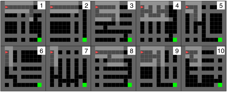
Figure 3: Sample environments.

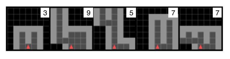
Figure 4: Sample queries labelled with targets corresponding to the environment which they were observed in.

All observations are provided as pixels to a standard convolutional backbone, with the corresponding agent location and direction appended to this representation and passed through an MLP head, equivalent to the procedure utilised for the adapted Meta-Dataset experiments. As a baseline comparison, we also train a Prototypical Network with an identical architecture on this task. Additionally, we train an equivalent recurrent network architecture typically applied to POMDP tasks such as this (Hausknecht & Stone, 2017), by adding a GRU layer (Cho et al., 2014; Chung et al., 2014) where the hidden state of the GRU is updated at each timestep and then extracted as the unified representation of the agent. We find that POEM trains more quickly and reaches almost 10% higher final environment recognition performance than both the Prototypical Network and GRU-based approach over 100 test episodes (81.1% vs 72.4% and 72.1%), as shown in appendix A.8. This is a result of POEM’s capacity to associate each observation with only part of the representation.

5.2 Reconstructing Environments from Partial Observation Trajectories

Having learned an environment encoder using the few-shot learning procedure above, we now investigate the extent to which our representations can be used to reconstruct the environment. As above, we generate trajectories with the optimal agent and feed these through the encoder to generate a representation of the environment. An MLP decoder is then trained to reconstruct the original environment layout from the learned environment representation. The decoder attempts to predict a one-hot representation of each possible grid cell, with a mean squared error loss. Given the trained encoder and decoder, we are now able to generate a map of the environment the optimal agent has traversed, solely from the agent’s partial observations, and without ever having seen the environment as a whole. A sample of environments alongside their reconstructions are shown in figure 5.

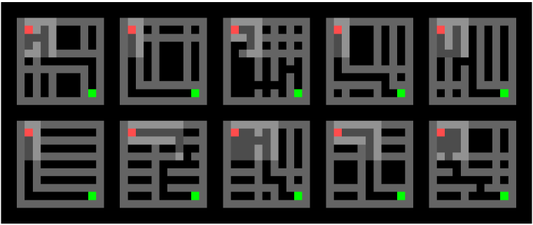
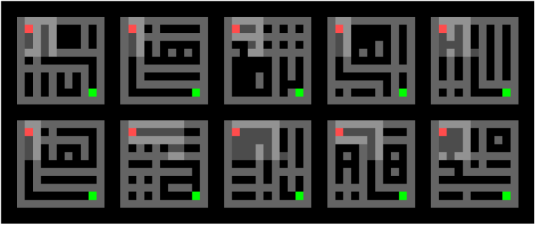
Figure 5: Left: Ground truth environments explored by the agent. Right: Reconstructions of the corresponding environments from POEM’s unified representation, encoded from the partial observations of the agent.

We see that the reconstructions clearly capture the approximate structure of each environment, demonstrating that the agent has been able to integrate its observations from along its trajectory into a single consistent representation. Since POEM enables the representation to be updated incrementally with each partial observation of the environment at inference time, it would be possible for an agent to update an internal environment representation at each step in its trajectory. There is potential for utilising this approach for learning environment representations to be beneficial in the context of exploration for reinforcement learning, but we leave such an investigation to future work.

6 Conclusion

In this work, we have introduced Partial Observation Experts Modelling (POEM), a contrastive meta-learning approach for few-shot learning in partially-observable settings. Unlike other standard contrastive and embedding-based meta-learning approaches, POEM utilises representational uncertainty to enable observations to inform only part of a representation vector. This probabilistic formalism enables consistent representation learning from multiple observations with a few-shot learning objective. We have demonstrated that POEM is comparable to the state-of-the-art baselines on a comprehensive few-shot learning benchmark, and outperforms these baselines when this benchmark is adapted to evaluate representation learning from partial observations. We have also demonstrated a promising potential application for POEM to learn representations of an environment from an agent’s partial observations. We hope that this research inspires further work into the challenging task of learning representations under partial observability and the creation of more realistic partial observability benchmarks.

Acknowledgments

Adam Jelley was kindly supported by Microsoft Research and EPSRC through Microsoft’s PhD Scholarship Programme. Antreas Antoniou was supported by a Huawei DDMPLab Innovation Research Grant. The Meta-Dataset experiments in this work were partly funded by Google Research Compute Credits, and we thank Hugo Larochelle for his support in acquiring these compute credits.

Appendix A Appendix

A.1 Gaussian Product Rules

Assuming the latent variable model $\phi(\mathbf{z}|\mathbf{x})$ to be a diagonal covariance multivariate Gaussian, the resulting integrals over latent variables become integrals over Gaussian products. This allows both $\lambda(\mathbf{y},\mathbf{X})$ (Equation 5) and $\lambda^{\prime}(\mathbf{X})$ (Equation 6) in the marginal predictive distribution (Equation 4) to be evaluated analytically using the following univariate Gaussian product rules on each independent dimension (Roweis, Sam, 1999).

Since a product of Gaussians $\prod_{i}N(\mu_{i},\tau_{i}^{-1})$ is itself a Gaussian, we have $\prod_{i}N(\mu_{i},\tau_{i}^{-1})=SN(\mu,\tau^{-1})$, where

$$\tau =\sum_{i}\tau_{i}$$ (8)

$$\mu =\frac{1}{\tau}\sum_{i}\tau_{i}\mu_{i}$$ (9)

$$S =(2\pi)^{\frac{(1-n)}{2}}\frac{\prod_{i}\tau_{i}^{1/2}}{\tau^{1/2}}\exp\left(\frac{1}{2}\tau\mu^{2}-\frac{1}{2}\sum_{i}\tau_{i}\mu_{i}^{2}\right).$$ (10)

Therefore the integral of a Gaussian product is given by the resulting normalisation $S$.

In the case of evaluating the marginal predictive distribution $p(\mathbf{x}^{*}|\mathbf{X}^{m})$ (equation 4), this gives $\frac{S^{*}S}{S^{\prime}S}=\frac{S^{*}}{S^{\prime}}$ where $S$ is the normalisation constant of the support product, $S^{*}$ is the normalisation constant of the product of the query and normalised support product, and $S^{\prime}$ is the normalisation constant of the product of the prior $p(z)$ and normalised support product. In reality, $p(z)$ generally has little impact as it is typically flat ($\tau\rightarrow 0$) over the region of non-negligible density of the product $\prod_{v=1}^{V}\phi(\mathbf{z}|\mathbf{x}_{v})$ and so $S^{\prime}\approx 1$ and we find $\frac{S^{*}}{S^{\prime}}\approx S^{*}$ so the ratios $\frac{\lambda}{\lambda^{\prime}}$ in the objective can be approximated by $S^{*}$, as in the simplified pseduocode in appendix A.3.

A.2 Derivation of Objective from Marginal Predictive Distribution

In section 3, we derived the marginal predictive distribution:

$$p(\mathbf{x}^{*}|\mathbf{X}^{m})=p(\mathbf{x}^{*})\frac{\lambda(\mathbf{x}^{*},\mathbf{X}^{m})}{\lambda^{\prime}(\mathbf{X}^{m})}$$ (11)

where

$$\lambda(\mathbf{y},\mathbf{X}) =\int d\mathbf{z}\ \phi(\mathbf{z}|\mathbf{y})\prod_{v=1}^{\mathrm{dim}(\mathbf{X})}\phi(\mathbf{z}|\mathbf{x}_{v}),\hskip 8.53581pt\mbox{ and}$$ (12)

$$\lambda^{\prime}(\mathbf{X}) =\int d\mathbf{z}\ p(\mathbf{z})\prod_{v=1}^{\mathrm{dim}(\mathbf{X})}\phi(\mathbf{z}|\mathbf{x}_{v}).$$ (13)

In our few shot task, the support data is chosen and then the query view is chosen uniformly at random to match the views of one of the support data items. Let the hypothesis $H_{m}$ indicate the event that the query view $\mathbf{x}^{*}$ comes from support point $m$. Then

$$P(H_{m}|S,\mathbf{x}^{*}) =\frac{P(H_{m})P(S,\mathbf{x}^{*}|H_{m})}{\sum_{m^{\prime}}P(H_{m^{\prime}})P(S,\mathbf{x}^{*}|H_{m^{\prime}})}=\frac{(1/M)p(\mathbf{x}^{*}|S,H_{m})}{\sum_{m^{\prime}}(1/M)p(\mathbf{x}^{*}|S,H_{m^{\prime}})}$$ (14)

$$=\frac{(1/M)p(\mathbf{x}^{*}|\mathbf{X}^{m})}{\sum_{m^{\prime}}(1/M)p(\mathbf{x}^{*}|\mathbf{X}^{m^{\prime}})}=\frac{p(\mathbf{x}^{*}|\mathbf{X}^{m})}{\sum_{m^{\prime}}p(\mathbf{x}^{*}|\mathbf{X}^{m^{\prime}})}.$$ (15)

From this we can formulate the training task: we wish to maximize the likelihood for the correct match of query point to support set, accumulated across all support/query selections from the dataset. Denote the $t$th support set by $S_{t}$, the $t$th query point by $x_{t}^{*}$, and let $m_{t}$ denote the support point with views that match the view of the query point. Then the complete negative log marginal likelihood objective to be minimized is:

$$\mathcal{L}(\{S_{t}\},\{x_{t}^{*}\}) =-\sum_{t}\log P(H_{m_{t}}|S_{t},\mathbf{x}_{t}^{*})$$ (16)

$$=-\sum_{t}\log\frac{p(\mathbf{x}^{*}|\mathbf{X}^{m})}{\sum_{m^{\prime}}p(\mathbf{x}^{*}|\mathbf{X}^{m^{\prime}})}$$ (17)

$$=-\sum_{t}\left[\log\frac{\lambda(\mathbf{x}^{*},\mathbf{X}^{m^{*}})}{\lambda^{\prime}(\mathbf{X}^{m^{*}})}-\log\sum_{m}\frac{\lambda(\mathbf{x}^{*},\mathbf{X}^{m})}{\lambda^{\prime}(\mathbf{X}^{m})}\right]$$ (18)

A.3 Pseudocode

Algorithm 1 Pytorch-Style Pseudocode: Gaussian Partial Observation Experts Modelling

⬇

# phi: dual-headed encoder network with shared backbone and output heads for mean and precision of Gaussian embedding

# M: Number of items/classes in task

# V: Number of views of each item/class (in general can vary with m in range(M))

# N: Number of query views

# D: Embedding dimension

# Load augmented partial views with view information

for (support_views, query_views, query_targets) in loader:

# support_views.shape = (M, V, ...)

# query_views.shape=(N, ...)

# query_targets.shape = (N,)

# Encode each support and query views

support_means, support_precisions = phi(support_views) # (M, V, D)

query_means, query_precisions = phi(query_views) # (N, D)

# Combine support views into unified representation of each item

# Gaussian products computed using equations in appendix A.1

# Optionally include prior Gaussian here (neglected for simplified implementation)

environment_means, environment_precisions, log_environment_normalisation = inner_gaussian_product(support_means, support_precisions) # Outputs: (M, D)

# Combine each query view with each unified support representation

env_query_mean, env_query_precisions, log_env_query_normalisation = outer_gaussian_product(support_means, support_precisions, query_means, query_precisions) # Outputs: (N, M, D)

# Predictions correspond to unified support with maximum overlap with query

_, predictions = log_env_query_normalisation.sum(2).max(1) # (N,)

# Cross entropy loss normalises with softmax and computes negative log-likelihood

loss = F.cross_entropy(log_env_query_normalisation, query_targets, reduction=’mean’)

# Optimization step

loss.backwards()

optimizer.step()

Algorithm 2 Language Agnostic Pseudocode: Gaussian Partial Observation Experts Modelling

1:Training meta-set $D^{train}\in\mathcal{T}$

2:Learning rate $\alpha$

3:Initialise dual-headed network $\phi_{\theta}(\mathbf{z}|\mathbf{x})$

4:$\triangleright$ Heads correspond to mean $\bm{\mu}$ and precision $\bm{\tau}$ of Gaussian embedding $\mathbf{z}$

5:while not converged do

6:     Sample task instance $\mathcal{T}_{i}=(\mathbf{X},\mathbf{x}^{*})\sim D^{train}$

7:$\triangleright$ Support set $\mathbf{X}$ consists of $V^{m}$ views of item $m\in\{1,...,M\}$.

8:$\triangleright$ Query set $\mathbf{x}^{*}$ consists of $N$ queries, each one view from any one item.

9:     Encode each view in support set $\mathbf{X}$ into Gaussian $\mathbf{z}$ using $\phi(\mathbf{z}|\mathbf{X})$

10:     Encode each query view in $\mathbf{x}^{*}$ into Gaussian $\mathbf{z}^{*}$ using $\phi(\mathbf{z}^{*}|\mathbf{x}^{*})$

11:     for $m\in\{1,...,M\}$ do

12:         Compute Gaussian product over views $\prod_{v=1}^{V^{m}}\phi(\mathbf{z}|\mathbf{x}_{v}^{m})$ (using results in A.1)

13:$\triangleright$ This gives unified support representation (global environment representation)

14:         for $n\in\{1,...,N\}$ do

15:              Compute Gaussian product of query with support product $\phi(\mathbf{z}_{n}^{*}|\mathbf{x}_{n}^{*})\prod_{v=1}^{V^{m}}\phi(\mathbf{z}|\mathbf{x}_{v}^{m})$

16:         end for

17:     end for

18:     Normalise resulting query-support normalisation constants $\overline{S^{m}_{n}}=\frac{S^{m}_{n}}{\sum_{m}S^{m}_{n}}$ across items

19:     Compute negative log of $\overline{S^{m^{*}}_{n}}$ for correct support as loss $\mathcal{L}(\{D_{t}\},\{x_{t}^{*}\})$ (eq.  7)

20:$\triangleright$ Negative log likelihood for correct support

21:     Perform gradient step w.r.t. $\theta$: $\theta\leftarrow\phi-\alpha\nabla_{\theta}\mathcal{L}(\{D_{t}\},\{x_{t}^{*}\})$

22:end while

A.4 Equivalence of Prototypical Network Objective to POEM Objective with Fixed Precisions

The probability of a query $\mathbf{x}^{*}$ belonging to class $n$ using the POEM objective is given by:

$$P(H_{m}|S,\mathbf{x}^{*})=\frac{\lambda(\mathbf{x}^{*};\mathbf{X}^{n})}{\lambda^{\prime}(\mathbf{X}^{n})}\bigg{/}\sum_{m}\frac{\lambda(\mathbf{x}^{*};\mathbf{X}^{m})}{\lambda^{\prime}(\mathbf{X}^{m})}$$ (19)

as defined in equation 15, where

$$\lambda(\mathbf{y},\mathbf{X}) =\int d\mathbf{z}\ \phi(\mathbf{z}|\mathbf{y})\prod_{v=1}^{V}\phi(\mathbf{z}|\mathbf{x}_{v}),\hskip 8.53581pt\mbox{ and}$$ (20)

$$\lambda^{\prime}(\mathbf{X}) =\int d\mathbf{z}\ p(\mathbf{z})\prod_{v=1}^{V}\phi(\mathbf{z}|\mathbf{x}_{v}).$$ (21)

.

Taking the precisions of the all Gaussian factors $\phi$ in $\lambda$ and $\lambda^{\prime}$ to be 1, we can apply the Gaussian product rules given in appendix A.1 to calculate $\lambda$ and $\lambda^{\prime}$ analytically. We find that this gives:

$$p_{n}=\frac{\frac{V_{n}}{V_{n}+1}^{\frac{1}{2}}\exp\left(-\frac{V_{n}}{2(V_{n}+1)}\left(\mu-\frac{\sum_{i}\mu_{ni}}{V_{n}}\right)^{2}\right)}{\sum_{m}\frac{V_{m}}{V_{m}+1}^{\frac{1}{2}}\exp\left(-\frac{V_{m}}{2(V_{m}+1)}\left(\mu-\frac{\sum_{i}\mu_{mi}}{V_{m}}\right)^{2}\right)}$$ (22)

where $\mu$ is the representation mean of the query, and $\mu_{ni}$ is the representation mean of support sample $i$ for class $n$, and $V_{n}$ is the number of support samples for class $n$.

Equivalently, the probability of a query with representation vector $\mu$ belonging to a class $n$ using a Prototypical Network objective is given by:

$$p_{n}=\frac{\exp\left(-\left(\mu-\frac{\sum_{i}\mu_{ni}}{V_{n}}\right)^{2}\right)}{\sum_{m}\exp\left(-\left(\mu-\frac{\sum_{i}\mu_{mi}}{V_{m}}\right)^{2}\right)}$$ (23)

We find that these are equivalent aside from the scaling factors $\frac{V_{m}}{(2)(V_{m}+1)}$ which only have a (significant) effect when there are varying numbers of samples by class, and a greater effect when the number of samples is smaller. Experimentally, we find that these scaling factors make little difference, as demonstrated in table 2 of section 4.3.

A.5 PO-Meta-Dataset Benchmark Additional Details

Parameters used for adapted PO-Meta-Dataset are provided in Table 3. All parameters not listed chosen to match Meta-Dataset defaults. All augmentations are applied using Torchvision, with parameters specified.

Table 3: PO-Meta-Dataset Parameters

PARAMETER	VALUE
Classes per Task	$[1,5]$
Samples per Task	$[5,25]$
Support Views per Sample	$18$
Query Views per Sample	$2$
Image Size	$(84,84)$ (except Omniglot, $(28,28)$)
Crop Size	$(14,14)$ ($1/6$ in each dim, except Omniglot, random placement)
Color Jitter	$(0.8,0.8,0.8,0.2)$, $p(apply)=0.3$
Random Greyscale	$0.2$
Random Horizontal Flip	$0.5$
Gaussian Blur	$((3,3),(1,0,2.0))$, $p(apply)=0.2$

All results computed over three runs. The Finetuning, Prototypical Network and POEM baselines were run on on-premise RTX2080 GPUs. MAML required more memory and compute than available, so was run on cloud A100s.

A.6 Relative Variance of Precisions During Training on Meta-Dataset and Meta-Meta-Dataset

The plot below shows the evolution of the variance in the representation precisions relative to the variance in the representation means learned by POEM on two distinct datasets, Aircraft and VGG Flowers. We see that for standard few-shot learning on Meta-Dataset, the variance in precisions is negligible relative to the variance in the means, demonstrating that the representational uncertainty is not useful in this task. Meanwhile, we see the variance in the precisions relative to the variance in the means becoming large before converging to a value of $\mathcal{O}(100)$ on the Meta-Meta-Dataset task, demonstrating that learning relative precisions is useful in this setting since each support sample only informs part of the representation.

A.7 Learning Representations of Environments Additional Details

Additional details about the parameters used for learning environment representations from agent observations are provided in Table 4

Table 4: Environment Representation Learning Parameters

PARAMETER	VALUE
Agent Training Algorithm	PPO (Schulman et al., 2017) (default hyperparameters)
Optimal Agent Reward	1 for reaching goal, -0.01 per timestep
Exploratory Agent Reward	1/N count exploration bonus (state defined by agent location and direction)
Encoder Conv Backbone Layers	5
Encoder MLP Head Layers	3
Encoder Embedding Dim	128 (corresponding $\sim 11\times 11$ environment size)
Decoder MLP Layers	4

A.8 Environment Recognition Accuracy During Training

POEM trains more quickly on the environment recognition task and reaches a higher final performance than an equivalent Prototypical Network or Recurrent Network (GRU) (81.1% vs 72.4% and 72.1% ) over a subsequent 100 test episodes.

References

- Antoniou et al. (2018) Antreas Antoniou, Harrison Edwards, and Amos Storkey. How to train your MAML. October 2018. doi: 10.48550/arXiv.1810.09502. URL https://arxiv.org/abs/1810.09502v3.
- Baz et al. (2021) Adrian El Baz, Isabelle Guyon, Zhengying Liu, Jan N. van Rijn, Sebastien Treguer, and Joaquin Vanschoren. Advances in MetaDL: AAAI 2021 Challenge and Workshop. In AAAI Workshop on Meta-Learning and MetaDL Challenge, pp. 1–16. PMLR, August 2021. URL https://proceedings.mlr.press/v140/el-baz21a.html. ISSN: 2640-3498.
- Baz et al. (2022) Adrian El Baz, Ihsan Ullah, Edesio Alcobaça, André C. P. L. F. Carvalho, Hong Chen, Fabio Ferreira, Henry Gouk, Chaoyu Guan, Isabelle Guyon, Timothy Hospedales, Shell Hu, Mike Huisman, Frank Hutter, Zhengying Liu, Felix Mohr, Ekrem Öztürk, Jan N. van Rijn, Haozhe Sun, Xin Wang, and Wenwu Zhu. Lessons learned from the NeurIPS 2021 MetaDL challenge: Backbone fine-tuning without episodic meta-learning dominates for few-shot learning image classification, July 2022. URL http://arxiv.org/abs/2206.08138. arXiv:2206.08138 [cs].
- Chen et al. (2020) Ting Chen, Simon Kornblith, Mohammad Norouzi, and Geoffrey Hinton. A Simple Framework for Contrastive Learning of Visual Representations. arXiv:2002.05709 [cs, stat], June 2020. URL http://arxiv.org/abs/2002.05709. arXiv: 2002.05709.
- Chen et al. (2021a) Wentao Chen, Chenyang Si, Wei Wang, Liang Wang, Zilei Wang, and Tieniu Tan. Few-Shot Learning with Part Discovery and Augmentation from Unlabeled Images, May 2021a. URL http://arxiv.org/abs/2105.11874. arXiv:2105.11874 [cs].
- Chen et al. (2021b) Yudong Chen, Chaoyu Guan, Zhikun Wei, Xin Wang, and Wenwu Zhu. MetaDelta: A Meta-Learning System for Few-shot Image Classification, February 2021b. URL http://arxiv.org/abs/2102.10744. arXiv:2102.10744 [cs].
- Chevalier-Boisvert et al. (2018) Maxime Chevalier-Boisvert, Lucas Willems, and Suman Pal. Minimalistic gridworld environment for OpenAI gym, 2018. URL https://github.com/maximecb/gym-minigrid.
- Cho et al. (2014) Kyunghyun Cho, Bart van Merrienboer, Dzmitry Bahdanau, and Yoshua Bengio. On the Properties of Neural Machine Translation: Encoder-Decoder Approaches, October 2014. URL http://arxiv.org/abs/1409.1259. arXiv:1409.1259 [cs, stat].
- Chung et al. (2014) Junyoung Chung, Caglar Gulcehre, KyungHyun Cho, and Yoshua Bengio. Empirical Evaluation of Gated Recurrent Neural Networks on Sequence Modeling, December 2014. URL http://arxiv.org/abs/1412.3555. arXiv:1412.3555 [cs].
- Cimpoi et al. (2014) Mircea Cimpoi, Subhransu Maji, Iasonas Kokkinos, Sammy Mohamed, and Andrea Vedaldi. Describing textures in the wild. In Proceedings of the IEEE conference on computer vision and pattern recognition, pp. 3606–3613, 2014.
- Dong et al. (2020) Chuanqi Dong, Wenbin Li, Jing Huo, Zheng Gu, and Yang Gao. Learning Task-aware Local Representations for Few-shot Learning. In Proceedings of the Twenty-Ninth International Joint Conference on Artificial Intelligence, pp. 716–722, Yokohama, Japan, July 2020. International Joint Conferences on Artificial Intelligence Organization. ISBN 978-0-9992411-6-5. doi: 10.24963/ijcai.2020/100. URL https://www.ijcai.org/proceedings/2020/100.
- Dumoulin et al. (2021) Vincent Dumoulin, Neil Houlsby, Utku Evci, Xiaohua Zhai, Ross Goroshin, Sylvain Gelly, and Hugo Larochelle. Comparing Transfer and Meta Learning Approaches on a Unified Few-Shot Classification Benchmark. Technical Report arXiv:2104.02638, arXiv, April 2021. URL http://arxiv.org/abs/2104.02638. arXiv:2104.02638 [cs] type: article.
- Edwards & Storkey (2017) Harrison Edwards and Amos Storkey. Towards a Neural Statistician. arXiv:1606.02185 [cs, stat], March 2017. URL http://arxiv.org/abs/1606.02185. arXiv: 1606.02185.
- Ericsson et al. (2021) Linus Ericsson, Henry Gouk, Chen Change Loy, and Timothy M. Hospedales. Self-Supervised Representation Learning: Introduction, Advances and Challenges. arXiv:2110.09327 [cs, stat], October 2021. URL http://arxiv.org/abs/2110.09327. arXiv: 2110.09327.
- Fernandez-Fernandez et al. (2019) Raul Fernandez-Fernandez, Juan G. Victores, David Estevez, and Carlos Balaguer. Quick, Stat!: A Statistical Analysis of the Quick, Draw! Dataset. In EUROSIM 2019 Abstract Volume, 2019. doi: 10.11128/arep.58. URL http://arxiv.org/abs/1907.06417. arXiv:1907.06417 [cs, eess].
- Finn et al. (2017) Chelsea Finn, Pieter Abbeel, and Sergey Levine. Model-Agnostic Meta-Learning for Fast Adaptation of Deep Networks. Technical report, 2017.
- Fürst et al. (2022) Andreas Fürst, Elisabeth Rumetshofer, Johannes Lehner, Viet Tran, Fei Tang, Hubert Ramsauer, David Kreil, Michael Kopp, Günter Klambauer, Angela Bitto-Nemling, and Sepp Hochreiter. CLOOB: Modern Hopfield Networks with InfoLOOB Outperform CLIP, November 2022. URL http://arxiv.org/abs/2110.11316. arXiv:2110.11316 [cs].
- Gordon et al. (2019) Jonathan Gordon, John Bronskill, Matthias Bauer, Sebastian Nowozin, and Richard E. Turner. Meta-Learning Probabilistic Inference For Prediction, August 2019. URL http://arxiv.org/abs/1805.09921. arXiv:1805.09921 [cs, stat].
- Hausknecht & Stone (2017) Matthew Hausknecht and Peter Stone. Deep Recurrent Q-Learning for Partially Observable MDPs. Technical Report arXiv:1507.06527, arXiv, January 2017. URL http://arxiv.org/abs/1507.06527. arXiv:1507.06527 [cs] type: article.
- He et al. (2015) Kaiming He, Xiangyu Zhang, Shaoqing Ren, and Jian Sun. Deep Residual Learning for Image Recognition. arXiv:1512.03385 [cs], December 2015. URL http://arxiv.org/abs/1512.03385. arXiv: 1512.03385.
- He et al. (2020) Kaiming He, Haoqi Fan, Yuxin Wu, Saining Xie, and Ross Girshick. Momentum Contrast for Unsupervised Visual Representation Learning. arXiv:1911.05722 [cs], March 2020. URL http://arxiv.org/abs/1911.05722. arXiv: 1911.05722.
- Hiller et al. (2022) Markus Hiller, Rongkai Ma, Mehrtash Harandi, and Tom Drummond. Rethinking Generalization in Few-Shot Classification, October 2022. URL http://arxiv.org/abs/2206.07267. arXiv:2206.07267 [cs].
- Hinton (2002) Geoffrey E Hinton. Training products of experts by minimizing contrastive divergence. Neural computation, 14(8):1771–1800, 2002. Publisher: MIT Press.
- Hospedales et al. (2020) Timothy Hospedales, Antreas Antoniou, Paul Micaelli, and Amos Storkey. Meta-Learning in Neural Networks: A Survey. April 2020. doi: 10.48550/arXiv.2004.05439. URL https://arxiv.org/abs/2004.05439v2.
- Lake et al. (2015) Brenden M Lake, Ruslan Salakhutdinov, and Joshua B Tenenbaum. Human-level concept learning through probabilistic program induction. Science (New York, N.Y.), 350(6266):1332–1338, 2015. Publisher: American Association for the Advancement of Science.
- Le-Khac et al. (2020) Phuc H. Le-Khac, Graham Healy, and Alan F. Smeaton. Contrastive Representation Learning: A Framework and Review. IEEE Access, 8:193907–193934, 2020. ISSN 2169-3536. doi: 10.1109/ACCESS.2020.3031549. URL http://arxiv.org/abs/2010.05113. arXiv: 2010.05113.
- Li et al. (2017) Zhenguo Li, Fengwei Zhou, Fei Chen, and Hang Li. Meta-sgd: Learning to learn quickly for few-shot learning. arXiv preprint arXiv:1707.09835, 2017.
- Lin et al. (2015) Tsung-Yi Lin, Michael Maire, Serge Belongie, Lubomir Bourdev, Ross Girshick, James Hays, Pietro Perona, Deva Ramanan, C. Lawrence Zitnick, and Piotr Dollár. Microsoft COCO: Common Objects in Context, February 2015. URL http://arxiv.org/abs/1405.0312. arXiv:1405.0312 [cs].
- Maji et al. (2013) Subhransu Maji, Esa Rahtu, Juho Kannala, Matthew Blaschko, and Andrea Vedaldi. Fine-Grained Visual Classification of Aircraft, June 2013. URL http://arxiv.org/abs/1306.5151. arXiv:1306.5151 [cs].
- Nakamura & Harada (2019) Akihiro Nakamura and Tatsuya Harada. Revisiting Fine-tuning for Few-shot Learning, October 2019. URL http://arxiv.org/abs/1910.00216. arXiv:1910.00216 [cs, stat].
- Nilsback & Zisserman (2008) Maria-Elena Nilsback and Andrew Zisserman. Automated flower classification over a large number of classes. In Indian conference on computer vision, graphics and image processing, December 2008.
- Oord et al. (2019) Aaron van den Oord, Yazhe Li, and Oriol Vinyals. Representation Learning with Contrastive Predictive Coding. arXiv:1807.03748 [cs, stat], January 2019. URL http://arxiv.org/abs/1807.03748. arXiv: 1807.03748.
- Paszke et al. (2019) Adam Paszke, Sam Gross, Francisco Massa, Adam Lerer, James Bradbury, Gregory Chanan, Trevor Killeen, Zeming Lin, Natalia Gimelshein, Luca Antiga, Alban Desmaison, Andreas Köpf, Edward Yang, Zach DeVito, Martin Raison, Alykhan Tejani, Sasank Chilamkurthy, Benoit Steiner, Lu Fang, Junjie Bai, and Soumith Chintala. PyTorch: An Imperative Style, High-Performance Deep Learning Library, December 2019. URL http://arxiv.org/abs/1912.01703. arXiv:1912.01703 [cs, stat].
- Patacchiola et al. (2020) Massimiliano Patacchiola, Jack Turner, Elliot J. Crowley, Michael O’Boyle, and Amos Storkey. Bayesian Meta-Learning for the Few-Shot Setting via Deep Kernels, October 2020. URL http://arxiv.org/abs/1910.05199. arXiv:1910.05199 [cs, stat].
- Radford et al. (2021) Alec Radford, Jong Wook Kim, Chris Hallacy, Aditya Ramesh, Gabriel Goh, Sandhini Agarwal, Girish Sastry, Amanda Askell, Pamela Mishkin, Jack Clark, Gretchen Krueger, and Ilya Sutskever. Learning Transferable Visual Models From Natural Language Supervision, February 2021. URL http://arxiv.org/abs/2103.00020. arXiv:2103.00020 [cs].
- Roweis, Sam (1999) Roweis, Sam. Gaussian Identities, 1999. URL https://cs.nyu.edu/~roweis/notes/gaussid.pdf.
- Russakovsky et al. (2015) Olga Russakovsky, Jia Deng, Hao Su, Jonathan Krause, Sanjeev Satheesh, Sean Ma, Zhiheng Huang, Andrej Karpathy, Aditya Khosla, Michael Bernstein, Alexander C. Berg, and Li Fei-Fei. ImageNet Large Scale Visual Recognition Challenge. arXiv:1409.0575 [cs], January 2015. URL http://arxiv.org/abs/1409.0575. arXiv: 1409.0575.
- Rusu et al. (2019) Andrei A. Rusu, Dushyant Rao, Jakub Sygnowski, Oriol Vinyals, Razvan Pascanu, Simon Osindero, and Raia Hadsell. Meta-Learning with Latent Embedding Optimization, March 2019. URL http://arxiv.org/abs/1807.05960. arXiv:1807.05960 [cs, stat].
- Schroeder, Brigit (2018) Schroeder, Brigit. FGVC5 - Fungi, 2018. URL https://sites.google.com/view/fgvc5/competitions/fgvcx/fungi.
- Schulman et al. (2017) John Schulman, Filip Wolski, Prafulla Dhariwal, Alec Radford, and Oleg Klimov. Proximal Policy Optimization Algorithms. arXiv:1707.06347 [cs], August 2017. URL http://arxiv.org/abs/1707.06347. arXiv: 1707.06347.
- Snell et al. (2017) Jake Snell, Kevin Swersky, and Richard S. Zemel. Prototypical Networks for Few-shot Learning. arXiv:1703.05175 [cs, stat], June 2017. URL http://arxiv.org/abs/1703.05175. arXiv: 1703.05175.
- Stallkamp et al. (2011) Johannes Stallkamp, Marc Schlipsing, Jan Salmen, and Christian Igel. The German traffic sign recognition benchmark: a multi-class classification competition. In The 2011 international joint conference on neural networks, pp. 1453–1460, 2011. tex.organization: IEEE.
- Sun et al. (2021) Zhuo Sun, Jijie Wu, Xiaoxu Li, Wenming Yang, and Jing-Hao Xue. Amortized Bayesian Prototype Meta-learning: A New Probabilistic Meta-learning Approach to Few-shot Image Classification. In Proceedings of The 24th International Conference on Artificial Intelligence and Statistics, pp. 1414–1422. PMLR, March 2021. URL https://proceedings.mlr.press/v130/sun21a.html. ISSN: 2640-3498.
- Sung et al. (2018) Flood Sung, Yongxin Yang, Li Zhang, Tao Xiang, Philip H. S. Torr, and Timothy M. Hospedales. Learning to Compare: Relation Network for Few-Shot Learning. Technical Report arXiv:1711.06025, arXiv, March 2018. URL http://arxiv.org/abs/1711.06025. arXiv:1711.06025 [cs] version: 2 type: article.
- Tang et al. (2012) Yichuan Tang, Ruslan Salakhutdinov, and Geoffrey Hinton. Deep Mixtures of Factor Analysers, June 2012. URL http://arxiv.org/abs/1206.4635. arXiv:1206.4635 [cs, stat].
- Triantafillou et al. (2020) Eleni Triantafillou, Tyler Zhu, Vincent Dumoulin, Pascal Lamblin, Utku Evci, Kelvin Xu, Ross Goroshin, Carles Gelada, Kevin Swersky, Pierre-Antoine Manzagol, and Hugo Larochelle. Meta-Dataset: A Dataset of Datasets for Learning to Learn from Few Examples. Technical Report arXiv:1903.03096, arXiv, April 2020. URL http://arxiv.org/abs/1903.03096. arXiv:1903.03096 [cs, stat] type: article.
- Vinyals et al. (2016) Oriol Vinyals, Charles Blundell, Timothy Lillicrap, koray kavukcuoglu, and Daan Wierstra. Matching Networks for One Shot Learning. In Advances in Neural Information Processing Systems, volume 29. Curran Associates, Inc., 2016. URL https://proceedings.neurips.cc/paper/2016/hash/90e1357833654983612fb05e3ec9148c-Abstract.html.
- Wah et al. (2011) Catherine Wah, Steve Branson, Peter Welinder, Pietro Perona, and Serge Belongie. The caltech-ucsd birds-200-2011 dataset. 2011. Publisher: California Institute of Technology.
- Williams et al. (2001) Christopher Williams, Felix Agakov, and Stephen Felderhof. Products of gaussians. In T. Dietterich, S. Becker, and Z. Ghahramani (eds.), Advances in Neural Information Processing Systems, volume 14. MIT Press, 2001. URL https://proceedings.neurips.cc/paper/2001/file/8232e119d8f59aa83050a741631803a6-Paper.pdf.
- Zhang et al. (2022) Chi Zhang, Yujun Cai, Guosheng Lin, and Chunhua Shen. DeepEMD: Differentiable Earth Mover’s Distance for Few-Shot Learning, January 2022. URL http://arxiv.org/abs/2003.06777. arXiv:2003.06777 [cs, eess].
- Zintgraf et al. (2019) Luisa M. Zintgraf, Kyriacos Shiarlis, Vitaly Kurin, Katja Hofmann, and Shimon Whiteson. Fast Context Adaptation via Meta-Learning. arXiv:1810.03642 [cs, stat], June 2019. URL http://arxiv.org/abs/1810.03642. arXiv: 1810.03642.