Multiple pion pair production in a Regge-based model

Abstract

Central diffractive event topologies at the LHC energies can be identified by two different approaches. First, the forward scattered protons can be measured in Roman pots. Second, a veto on hadronic activity away from midrapidity can be imposed to define a double-gap topology. Such a double-gap topology trigger has been implemented by the ALICE collaboration in Run 1 and Run 2 of the LHC. The analysis of these events allows to determine the charged-particle multiplicity within the acceptance. The excellent particle identification capabilities of ALICE allows to study two-track events both in the pion and kaon sector. Events with measured charged particle multiplicity larger than two can arise from multiple pair production. A Regge-based approach for modeling such multiple pair production is presented.

1 Introduction

Double-Pomeron fusion at hadron colliders results in a double-gap event topology. Such a topology is defined by hadronic activity at or close to midrapidity, and the absence thereof away from midrapidity. The multiplicity distribution of such double-gap events has been measured in the ALICE central barrel. To better understand such multiplicity distributions we present here a Regge-based approach for multiple pion pair production in double-Pomeron events. This model is based on a Dual Amplitude with Mandelstam Analyticity (DAMA) [1]. In this approach, the production of multiple pairs can be modeled by including a Pomeron-Pomeron-Reggeon and a triple-Pomeron coupling. The amplitude at Pomeron level within his DAMA formulation is given, and the resulting mass distributions for double pion and double b-resonance production are shown.

2 Multiplicity distribution of double-gap events

The charged-particle multiplicity in the ALICE central barrel has been analyzed in LHC Run 1 for both minimum bias and double-gap events [2].

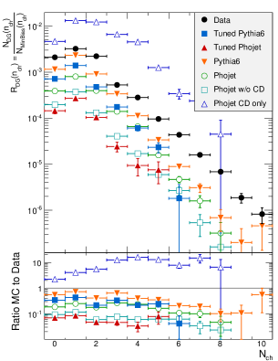
Figure 1: Double-gap probability in ALICE central barrel as function of charged-particle multiplicity (Figure taken from Ref. [2]).

In Fig. 1, the probability of being a double-gap event is shown as function of the charged-particle multiplicity N_ch in the ALICE central barrel. The ALICE data are shown in black circles, whereas the results from Monte Carlo generators are shown in different colors. These probabilities clearly show a maximum at N_ch=1 and N_ch=2, demonstrating that double-Pomeron events are dominated by very low multiplicities as compared to minimum bias events. As indicated in this figure, none of the tested generators shows reasonable agreement with the data. This discrepancy between the ALICE measured double-gap events and the prediction of the tested generators motivates the development of a model which can be used to analyze unlike-sign two-track events resulting from single resonance decays, as well as the higher-multiplicity events stemming from the decays of multiple resonances.

3 A Regge model for double-Pomeron events

The model for Pomeron-Pomeron-induced events presented in the following is based on the DAMA approach. Pomeron-induced single-resonance production has been presented in our previous studies [3, 4]. Here, we extend this DAMA approach to the production of multiple resonances.

\begin{overpic}[width=390.25534pt]{single_reg.pdf} \end{overpic}

\begin{overpic}[width=104.07117pt]{empty.pdf} \put(6.0,20.0){\vector(1,0){14.0}} \put(5.0,13.0){amplitude} \put(4.5,8.8){subdiagram} \end{overpic}

\begin{overpic}[width=390.25534pt]{single_reg_red.pdf} \end{overpic}

Figure 2: Amplitude at hadron level (left), and Pomeron subdiagram (right).

In Fig. 2, the amplitude for Pomeron-induced single-resonance production at hadron level is shown on the left. The subdiagram on the right represents the amplitude for Pomeron-Pomeron $\rightarrow$ resonance. The cross section at hadron level is derived by convoluting the subdiagram cross section with the Pomeron flux of the proton $F^{\mathbb{P}}_{\text{prot}}(t,\xi)$ defined by

$$F^{\mathbb{P}}_{\text{prot}}(t,\xi)=\frac{9\beta^{2}_{0}}{4\pi^{2}}[F_{1}(t)]^{2}\xi^{1-2\alpha(t)},$$ (1)

with $F_{1}(t)$ the elastic form factor, and $\alpha(t)$ the Pomeron trajectory [3].

In the DAMA approach, multiple-resonance production can be modeled by introducing a Pomeron-Pomeron-Reggeon ($\mathbb{P}\mathbb{P}\mathbb{R}$) coupling with subsequent splitting of the intermediate Reggeon into the two final-state Reggeons. Alternatively, the same final state can be formed by a triple-Pomeron ($\mathbb{P}\mathbb{P}\mathbb{P}$) coupling with the intermediate Pomeron decaying into the two Reggeons.

\begin{overpic}[width=34.69038pt]{empty.pdf} \end{overpic}

\begin{overpic}[width=407.60385pt]{triple_reg_red.pdf} \put(3.0,30.0){$\alpha_{\mathbb{P}}$} \put(10.0,37.0){t${}_{1}$} \put(2.0,10.0){$\alpha_{\mathbb{P}}$} \put(10.0,6.0){t${}_{2}$} \put(6.0,23.0){g${}_{1}$} \put(36.0,23.0){g${}_{2}$} \put(-5.0,23.6){\vector(1,0){8.0}} \put(-7.2,22.8){$\tilde{s}$} \put(18.0,26.0){$\alpha_{\mathbb{R}}(\tilde{s})$} \put(22.8,37.6){\vector(0,-1){8.0}} \put(22.0,38.8){$\tilde{t}$} \put(49.0,21.6){{\Huge+}} \put(38.0,38.0){$\tilde{S}_{1}(M^{2}_{1})$} \put(37.0,7.0){$\tilde{S}_{2}(M^{2}_{2})$} \put(-14.0,18.0){\large{($\tilde{s}\!=\!t_{1}\!+\!t_{2}$)}} \end{overpic}

\begin{overpic}[width=407.60385pt]{triple_pom_red.pdf} \put(6.0,23.4){g${}_{3}$} \put(36.0,23.4){g${}_{4}$} \put(19.0,27.0){$\alpha_{\mathbb{P}}(\tilde{s})$} \put(38.0,38.0){$\tilde{S}_{1}(M^{2}_{1})$} \put(38.0,7.0){$\tilde{S}_{2}(M^{2}_{2})$} \end{overpic}

Figure 3: Subdiagram for $\mathbb{P}\mathbb{P}\mathbb{R}$ amplitude (left), and $\mathbb{P}\mathbb{P}\mathbb{P}$ amplitude (right).

The DAMA amplitude for the subdiagram shown in Fig. 3 is given by

$$A_{\mathbb{P}\mathbb{P}\rightarrow\tilde{S}_{1}\tilde{S}_{2}}(\tilde{s},\tilde{t},M^{2}_{1},M^{2}_{2}))=\frac{1}{\sqrt{M^{2}_{1}M^{2}_{2}}}\sum_{\mathbb{P}\mathbb{P}\mathbb{R},\mathbb{P}\mathbb{P}\mathbb{P}}\sum_{n}\frac{g_{i}g_{j}e^{b\alpha(\tilde{t})}}{n-\alpha(\tilde{s})},$$ (2)

with the first summation over the two amplitudes of Fig. 3 defined by the $\mathbb{P}\mathbb{P}\mathbb{R}$ coupling with g_i,g_j=g₁,g₂, and the $\mathbb{P}\mathbb{P}\mathbb{P}$ coupling with g_i,g_j=g₃,g₄. The index $n$ sums over the spins of the resonances of the intermediate trajectory which connects the vertices $i,j$. From this amplitude, the cross section at Pomeron level is derived by the optical theorem

$$\sigma_{t}(\tilde{s},M^{2}_{1},M^{2}_{2})=\Im m\;A(\tilde{s},\tilde{t}\!=\!0,M^{2}_{1},M^{2}_{2}),$$ (3)

with the imaginary part of $A(\tilde{s},\tilde{t},M^{2}_{1},M^{2}_{2})$ defined by $\alpha_{\mathbb{R}}(\tilde{s})$ and $\alpha_{\mathbb{P}}(\tilde{s})$ for the $\mathbb{P}\mathbb{P}\mathbb{R}$ and the $\mathbb{P}\mathbb{P}\mathbb{P}$ diagrams of Fig. 3, respectively.

4 Reggeizing $q\bar{q}$ states in the light quark sector

The final-state mesons derive from the decay of the meson resonances lying on the two Regge trajectories $\tilde{S}_{1}$ and $\tilde{S}_{2}$ as illustrated in Fig. 3. In order to be able to include mesonic bound states of different radial and orbital excitations, a unified description of $q\bar{q}$ bound states in the different flavour sectors is needed. Such a unified description of $q\bar{q}$ bound states including a confinement potential, a spin-orbit, a hyperfine and an annihilation interaction is presented in Ref. [5]. The solutions for these $q\bar{q}$ bound states are given in spectroscopic notation $n\>^{2S+1}L_{J}$.

spectr. notation $n\>^{2S+1}L_{J}$:
- $n$ radial quantum number
- $S$ spin
- $L$ orbital ang. momentum
- $J$ total ang. momentum

$n\>^{2S+1}L_{J}$	mass	PDG	mass	width
	Ref. [5]		(PDG)	(PDG)
$1^{1}S_{0}$	150	$\pi$	140	0
$1^{1}P_{1}$	1220	$b_{1}$	1230	142
$1^{1}D_{2}$	1680	$\pi_{2}$	1672	258
$1^{1}F_{3}$	2030	——	——	——
$1^{1}G_{4}$	2330	——	——	——

Table 1: Masses and widths in MeV.

In Table 1, masses are presented for the isovector channel in the light quark sector for the radial ground state for S,P,D,F and G-wave, and are compared to the values given by the Particle Data Group [6]. The S- and D-wave bound states calculated in Ref. [5] are identified with the $\pi$ and the $\pi_{2}$ states of mass 140 and 1672 MeV, respectively. The P-wave solution is associated to the known $b_{1}$ state of mass 1230 MeV. No candidates for the predicted F- and G-wave bound states have so far been experimentally identified [6].

5 Non-linear complex Regge trajectory

The small but existing non-linear dependence of the spin of a resonance to its mass squared can be used to make a Regge trajectory $\alpha(M^{2})$ a complex entity with real and imaginary parts being related by a dispersion relation [7]. Here, the real part is defined by the value of the spin, and the imaginary part is related to the decay width $\Gamma$ by $\Im m\>\alpha(M_{R}^{2})=\Gamma(M_{R})\>\alpha^{{}^{\prime}}\>M_{R}$, with $\alpha^{{}^{\prime}}$ denoting the derivative of the real part of the trajectory. In a simple model, the imaginary part is chosen as a sum of single threshold terms

$$\Im m\>\alpha(s)\!=\!\sum_{n}\!c_{n}(s\!-\!s_{n})^{1/2}\big{(}\frac{s\!-\!s_{n}}{s}\big{)}^{\!|\Re e\>\alpha(s_{n})|}\theta(s\!-\!s_{n}).$$ (4)

In Eq. 4, the coefficients $c_{n}$ are fit parameters, and the parameters $s_{n}$ represent kinematical thresholds of decay channels.

5.1 The ($\pi,b$)-trajectory

A Regge trajectory, called the ($\pi,b$)-trajectory hereafter, is defined by the values of mass and width of the S, P and D-waves shown in Table 1.

\begin{overpic}[width=208.13574pt]{pion_real_prune.pdf} \put(6.0,27.8){{\color[rgb]{1,0,0}-}}\put(7.6,27.8){{\color[rgb]{1,0,0}-}}\put(9.2,27.8){{\color[rgb]{1,0,0}-}}\put(10.8,27.8){{\color[rgb]{1,0,0}-}}\put(12.4,27.8){{\color[rgb]{1,0,0}-}}\put(14.0,27.8){{\color[rgb]{1,0,0}-}}\put(15.6,27.8){{\color[rgb]{1,0,0}-}}\put(17.2,27.8){{\color[rgb]{1,0,0}-}}\put(18.8,27.8){{\color[rgb]{1,0,0}-}}\put(20.4,27.8){{\color[rgb]{1,0,0}-}}\put(22.0,27.8){{\color[rgb]{1,0,0}-}}\put(23.6,27.8){{\color[rgb]{1,0,0}-}}\put(25.2,27.8){{\color[rgb]{1,0,0}-}}\put(26.8,27.8){{\color[rgb]{1,0,0}-}}\put(28.4,27.8){{\color[rgb]{1,0,0}-}}\put(30.0,27.8){{\color[rgb]{1,0,0}-}} \put(6.0,35.45){{\color[rgb]{1,0,0}-}}\put(7.6,35.45){{\color[rgb]{1,0,0}-}}\put(9.2,35.45){{\color[rgb]{1,0,0}-}}\put(10.8,35.45){{\color[rgb]{1,0,0}-}}\put(12.4,35.45){{\color[rgb]{1,0,0}-}}\put(14.0,35.45){{\color[rgb]{1,0,0}-}}\put(15.6,35.45){{\color[rgb]{1,0,0}-}}\put(17.2,35.45){{\color[rgb]{1,0,0}-}}\put(18.8,35.45){{\color[rgb]{1,0,0}-}}\put(20.4,35.45){{\color[rgb]{1,0,0}-}}\put(22.0,35.45){{\color[rgb]{1,0,0}-}}\put(23.6,35.45){{\color[rgb]{1,0,0}-}}\put(25.2,35.45){{\color[rgb]{1,0,0}-}}\put(26.8,35.45){{\color[rgb]{1,0,0}-}}\put(28.4,35.45){{\color[rgb]{1,0,0}-}}\put(30.0,35.45){{\color[rgb]{1,0,0}-}}\put(31.6,35.45){{\color[rgb]{1,0,0}-}}\put(33.2,35.45){{\color[rgb]{1,0,0}-}}\put(34.8,35.45){{\color[rgb]{1,0,0}-}}\put(36.4,35.45){{\color[rgb]{1,0,0}-}}\put(38.0,35.45){{\color[rgb]{1,0,0}-}}\put(39.6,35.45){{\color[rgb]{1,0,0}-}} \put(6.0,43.1){{\color[rgb]{1,0,0}-}}\put(7.6,43.1){{\color[rgb]{1,0,0}-}}\put(9.2,43.1){{\color[rgb]{1,0,0}-}}\put(10.8,43.1){{\color[rgb]{1,0,0}-}}\put(12.4,43.1){{\color[rgb]{1,0,0}-}}\put(14.0,43.1){{\color[rgb]{1,0,0}-}}\put(15.6,43.1){{\color[rgb]{1,0,0}-}}\put(17.2,43.1){{\color[rgb]{1,0,0}-}}\put(18.8,43.1){{\color[rgb]{1,0,0}-}}\put(20.4,43.1){{\color[rgb]{1,0,0}-}}\put(22.0,43.1){{\color[rgb]{1,0,0}-}}\put(23.6,43.1){{\color[rgb]{1,0,0}-}}\put(25.2,43.1){{\color[rgb]{1,0,0}-}}\put(26.8,43.1){{\color[rgb]{1,0,0}-}}\put(28.4,43.1){{\color[rgb]{1,0,0}-}}\put(30.0,43.1){{\color[rgb]{1,0,0}-}}\put(31.6,43.1){{\color[rgb]{1,0,0}-}}\put(33.2,43.1){{\color[rgb]{1,0,0}-}}\put(34.8,43.1){{\color[rgb]{1,0,0}-}}\put(36.4,43.1){{\color[rgb]{1,0,0}-}}\put(38.0,43.1){{\color[rgb]{1,0,0}-}}\put(39.6,43.1){{\color[rgb]{1,0,0}-}}\put(41.2,43.1){{\color[rgb]{1,0,0}-}}\put(42.8,43.1){{\color[rgb]{1,0,0}-}}\put(44.4,43.1){{\color[rgb]{1,0,0}-}}\put(46.0,43.1){{\color[rgb]{1,0,0}-}}\put(47.6,43.1){{\color[rgb]{1,0,0}-}}\put(49.2,43.1){{\color[rgb]{1,0,0}-}} \put(31.8,28.6){{\color[rgb]{1,0,0}\circle{1.2}}} \put(41.2,36.2){{\color[rgb]{1,0,0}\circle{1.2}}} \put(50.7,43.9){{\color[rgb]{1,0,0}\circle{1.2}}} \put(8.2,6.5){{\color[rgb]{0,0,1}\footnotesize{$\pi$}}} \put(15.9,12.4){{\color[rgb]{0,0,1}\footnotesize{$b_{1}$}}} \put(23.8,20.2){{\color[rgb]{0,0,1}\footnotesize{$\pi_{2}$}}} \put(33.2,27.4){{\color[rgb]{1,0,0}\footnotesize{$b_{3}$}}} \put(42.2,35.3){{\color[rgb]{1,0,0}\footnotesize{$\pi_{4}$}}} \put(50.8,40.8){{\color[rgb]{1,0,0}\footnotesize{$b_{5}$}}} \end{overpic}\begin{overpic}[width=208.13574pt]{pion_width_prune.pdf} \put(4.2,6.6){{\color[rgb]{0,0,1}\footnotesize{$\pi$}}} \put(16.2,21.0){{\color[rgb]{0,0,1}\footnotesize{$b_{1}$}}} \put(23.6,34.4){{\color[rgb]{0,0,1}\footnotesize{$\pi_{2}$}}} \put(6.6,2.0){{\color[rgb]{1,0,0}\line(0,1){3.6}}} \put(13.5,2.0){{\color[rgb]{1,0,0}\line(0,1){3.6}}} \put(5.2,-0.5){\small\color[rgb]{1,0,0}$s_{0}$} \put(12.2,-0.5){\small\color[rgb]{1,0,0}$s_{1}$} \end{overpic}

Figure 4: Real part $(\pi,b)$-trajectory on the left, width function $\Gamma$ on the right.

In Fig. 4 on the left, the three data points of the $\pi,b_{1}$ and $\pi_{2}$ states are shown by black points, and the non-linear fit by the blue line. On the right, the widths of the $\pi,b_{1}$ and $\pi_{2}$ states are shown by black points, and the fitted width function $\Gamma$ by the blue line. The thresholds $s_{0}$ and $s_{1}$ used in the fit of Eq. 4 are shown in red. The thresholds $s_{0}$=0.176 GeV² and $s_{1}$=1.27 GeV² are defined by the decays $\pi_{2}\!\rightarrow\!3\pi$ and $b_{1}\!\rightarrow\!K\bar{K}\pi$, respectively. This fit of the ($\pi,b$)-trajectory predicts a $b_{3}$ state with mass of 2090 MeV and width of 321 MeV, a $\pi_{4}$ state with mass of 2437 MeV and width of 352 MeV, and a $b_{5}$ state with mass of 2738 MeV and width of 371 MeV.

6 The final-state resonance mass distribution

The ($\pi,b$)-trajectory consists of $\pi$ and $b$-resonances with quantum numbers (P,C)=($-,+$), and (P,C)=($+,-$), respectively. The final state shown in Fig. 3 can hence contain two $\pi$-resonances, or two $b$-resonances.

\begin{overpic}[width=190.79385pt]{pion_mass2d_fac_prune.pdf} \put(16.0,-0.4){\tiny PC=(-,+)} \put(46.0,4.0){\rotatebox{16.0}{\tiny$M^{2}_{1}(\tilde{S}^{\pi}_{1})$}} \put(2.0,11.0){\rotatebox{-30.0}{\tiny$M^{2}_{2}(\tilde{S}^{\pi}_{2})$}} \put(-3.0,28.0){\rotatebox{90.0}{\small arb. units}} \end{overpic}\begin{overpic}[width=195.12767pt]{bres_mass2d_fac_prune.pdf} \put(16.0,-0.4){\tiny PC=(+,-)} \put(46.0,4.0){\rotatebox{16.0}{\tiny$M^{2}_{1}(\tilde{S}^{b}_{1})$}} \put(2.0,11.0){\rotatebox{-30.0}{\tiny$M^{2}_{2}(\tilde{S}^{b}_{2})$}} \put(-2.0,28.0){\rotatebox{90.0}{\small arb. units}} \end{overpic}

Figure 5: Two-dimensional mass distribution of the final-state resonances.

In Fig. 5, the two-dimensional distribution of squared masses is shown for $\tilde{s}$ = 9 GeV² for the case of two $\pi$-resonances on the left, and the corresponding distribution for two $b$-resonances on the right. Here, $\tilde{s}$ denotes the center-of-mass energy of the two initial-state Pomerons as shown in Fig. 3.

7 Acknowledgements

This work is supported by the German Federal Ministry of Education and Research under reference 05P21VHCA1. An EMMI visiting Professorship at the University of Heidelberg is gratefully acknowledged by L.J.

References

• [1] A.I.Bugrji etΒ al. Dual Amplitudes with Mandelstam Analyticity. Fortschr. Phys. 21, 427, 1973.
• [2] F.Reidt. Analysis of Double-Gap Events in Proton-Proton Collisions at $\sqrt{s}$ = 7 TeV with ALICE at the LHC. Master thesis, University Heidelberg, 2012.
• [3] R.Schicker R.Fiore, L.Jenkovszky. Resonance production in Pomeron-Pomeron collisions at the LHC. Eur.Phys.J.C 76, 1, 38, 2016.
• [4] R.Schicker R.Fiore, L.Jenkovszky. Exclusive diffractive resonance production in proton-proton collisions at high energies. Eur.Phys.J.C 78, 6, 468, 2018.
• [5] N.Isgur S.Godfrey. Mesons in a Relativized Quark Model with Chromodynamics. Phys.Rev.D 32, 189, 1985.
• [6] P.A.Zyla etΒ al. Particle Data Group. Prog.Theor.Exp.Phys. 2020, 083C01.
• [7] E.Predazzi A.Degasperis. Dynamical Calculation of Regge Trajectories. Nuovo Cim. Vol.A 65, 764, 1970.