A Herschel study of the high-mass protostar IRAS 20126+4104

We performed Herschel observations of the continuum and line emission from the high-mass star-forming region IRAS 20126+4104, which hosts a well-studied B-type (proto)star powering a bipolar outflow and is associated with a Keplerian circumstellar disk. The continuum images at six wavelengths allowed us to derive an accurate estimate of the bolometric luminosity and mass of the molecular clump enshrouding the disk. The same region has been mapped in 12 rotational transitions of carbon monoxide, which were used in synergy with the continuum data to determine the temperature and density distribution inside the clump and improve upon the mass estimate. The maps of two fine structure oxygen far-IR lines were used to estimate the volume density of the shocked region at the surface of the southern lobe of the outflow and the mass-loss rate. Our findings lend further support to the scenario previously proposed by various authors, confirming that at the origin of the bolometric luminosity and bipolar outflow from IRAS 20126+4104 is a B-type star located at the centre of the Keplerian disk.

1 Introduction

The study of massive stars (conventionally those in excess of $\sim$8 $M_{\odot}$) is hampered by various problems, the most important of which probably being their large distances and their formation in clusters. As a consequence, precise estimates of crucial physical quantities such as the stellar luminosity in addition to accretion and outflow rates had been difficult to obtain until recently. With the substantial improvement of sensitivity and angular resolution provided by the new instruments that have recently become available online, these limitations can be overcome, at least in part. In this study we exploit the potential of the ESA Herschel Space Observatory (Pilbratt et al. pilb (2010)) to image the continuum and line emission from a massive (proto)star in the far-IR at a few 10″ resolution in the wake of previous studies by other authors (e.g. Green et al. green13 (2013); Manoj et al. manoj13 (2013, 2016); Karska et al. karska13 (2013, 2013, 2013); Nisini et al. nisi (2015); Mottram et al. mott17 (2017); Yang et al. yang18 (2018)). In particular, the fine structure Oi line at 63 $\mu$m has been found to be tightly associated with outflows in both low-mass (Kristensen et al. krist17 (2017); Yang et al. yang22 (2022)) and high-mass (Schneider et al. schnei18 (2018)) young stellar objects (YSOs), although it is possibly affected (especially at low velocities) by absorption in foreground clouds (Leurini et al. leu15 (2015)).

The target of our study is the well-known massive (proto)star IRAS 20126+4104. This object was probably the first Keplerian disk found around a massive (proto)star and it has been extensively studied over almost the entire electromagnetic spectrum accessible to the observers, from the radio to the X-ray domain. While it would be too lengthy to review all the results obtained, here we mention the most relevant to the present study.

The (proto)star lies at the centre of a disk, which was first detected by Cesaroni et al. (cesa97 (1997)) and confirmed by subsequent higher-resolution studies (Zhang et al. zha98 (1998); Cesaroni et al. cesa99 (1999, 2005, 2014)). Sub-arcsecond imaging (Cesaroni et al. cesa14 (2014)) and model fitting (Chen et al. chen (2019)) have proved that the disk is undergoing Keplerian rotation about a $\sim$$12\leavevmode\nobreak\ M_{\odot}$ (proto)star, as suggested by the butterfly-shaped position–velocity plot obtained in almost any hot molecular core tracer observed. Evidence of accretion onto the (proto)star has also been reported (Cesaroni et al. cesa99 (1999); Keto & Zhang ketzha (2010); Johnston et al. johns (2011)). The (proto)star is powering a outflow undergoing precession about the disk axis (Shepherd et al. shep (2000); Cesaroni et al. cesa05 (2005); Caratti o Garatti et al. caga08 (2008)). This outflow has been imaged on scales from a few 100 au (Moscadelli et al. mosca05 (2005); Cesaroni et al. cesa13 (2013)) to 0.5 pc (Shepherd et al. shep (2000); Lebrón et al. lebr (2006)) and its 3D expansion velocity has been measured through maser and H₂-knot proper motions (Moscadelli et al. mosca05 (2005); Massi et al. massi23 (2023)). The distance to IRAS 20126+4104 (1.64$\pm$0.05 kpc) has been accurately determined from parallax measurements of the H₂O masers (Moscadelli et al. mosca11 (2011)), which prove this to be one of the closest disks around B-type (proto)stars, thus allowing for excellent linear resolution. More recently, Nagayama et al. (naga15 (2015)) have repeated the parallax measurement with the Japanese Very-Long-Baseline Interferometry (VLBI) Exploration of Radio Astrometry (VERA) resulting in a distance of 1.33${}^{+0.19}_{-0.092}$ kpc, consistent with the value of Moscadelli et al. within the uncertainties. For our study we adopt the distance estimate with the minimum error, that is 1.64 kpc. Imaging at IR wavelengths (Qiu et al. qiu08 (2008)) seemed to indicate that IRAS 20126+4104 is associated with an anomalously poor stellar cluster. However, subsequent X-ray observations by Montes et al. (montes (2015)) have revealed an embedded stellar population that hints at the existence of a richer (and possibly very young) cluster.

The aim of this paper is to obtain precise estimates of the luminosity and outflow mass-loss rate, which are necessary to shed light on the stellar properties and possible stellar multiplicity. We also want to establish the origin of the Oi line emission and use it to obtain an alternative estimate of the mass-loss rate in the jet. With this in mind, we performed Herschel observations of the continuum and line emission from IRAS 20126+4104.

This paper is organized as follows. In Sect. 2 the observations and data reduction procedures are described. In Sect. 3 we outline the results obtained, which are then analysed and discussed in Sect. 4. Finally, the conclusions are drawn in Sect. 5.

2 Observations and data reduction

We observed a total time of 11.5 hours with the Photodetector Array Camera and Spectrometer (PACS; Poglitsch et al. pogl (2010)) and the Spectral and Photometric Imaging Receiver (SPIRE; Griffin et al. griff (2010)), to cover a region of at least 2′$\times$2′ centred on IRAS 20126+4104. The photometric and spectroscopic data are described separately in the following sections.

2.1 Photometry

2.1.1 Data acquisition

We obtained observations in photometric mode with both PACS and SPIRE of an area similar to that mapped in spectroscopic mode. Continuum maps of the region were made in six bands at 70, 100, 110, 160, 250, 350, and 500 $\mu$m. A single coverage was sufficient at all bands due to the strong source intensity.

SPIRE was used in mini-map mode, employing a small scan map using the nearly orthogonal scan paths, with a fixed scan angle (42° with respect to the z-axis of the spacecraft) and scan speed (30″/s), resulting in a circular coverage of 5′ diameter. PACS was used in scan-map mode to map a region of about 3′$\times$3′. Two coverages were necessary for all three PACS bands, implying a time of 558 sec. A mini map was obtained by moving the array with a constant speed of 20″/s along four parallel legs, with small leg separation (2″–5″). The length of the legs was 3′. Scanning was performed in array coordinates at 70°/110°, in order to align the scan direction along the diagonal of the array. To improve the sensitivity and better image extended sources, two consecutive orthogonal mini scan-maps were acquired. The obtained map shows a central homogeneous, high-coverage area with a diameter of 50″. The execution time of a mini map composed by the concatenation of two quasi-orthogonal directions was 567 second (for six scan legs with a separation of 4″ and leg length of 3′), of which 104 seconds were effectively spent on the source.

2.1.2 Data reduction

The standard products were obtained by performing queries at the Herschel Science Archive (HSA), using jython (java+python) scripts developed within the Herschel Interactive Processing Environment (HIPE; Ott ott (2010)). The level 2 standard products were extracted from the observational context and were processed with dedicated scripts to optimize the results and completely remove the residual features.

The raw data acquired with the SPIRE mini-map mode, at 250, 350, and 500 $\mu$m, contain both orthogonal scan directions in a single observation. The standard pipeline combines all the scan directions, producing a single observation. For our study, we used the level 2 standard products.

For maps acquired with PACS, every scan direction corresponds to a single observation; therefore, all of the observations had to be combined to obtain a map. For this purpose, a specific pipeline was created that uses the level 0 time ordered data (TOD) from the HSA, after removing all of the instrumental and observational effects, such as Glitch, drift, offset, and 1/f noise. Our pipeline produces one map for each PACS band (70, 100, 110, and 160 $\mu$m). For our study we used these reprocessed data.

2.2 Spectroscopy

2.2.1 Data acquisition

PACS was used in spectroscopic mode to build a raster map of a region of 2′$\times$2′ centred on RA=20^h14^m25$\aas@@fstack{s}$5 Dec=41°13′10″ in five lines: Oi 63 $\mu$m, Oi 145 $\mu$m, Cii 157 $\mu$m, ¹²CO $J$=18$\rightarrow$17 at 145 $\mu$m, H₂O $2_{2,1}$–$1_{1,0}$ at 108 $\mu$m, and ¹²CO $J$=24$\rightarrow 23$ at 109 $\mu$m. The total integration time was 14867 sec. SPIRE was used in single pointing spectral mode with an intermediate coverage and high resolution to obtain the interferogram in the band from 194 $\mu$m to 672 $\mu$m, with the aim to map the same area as PACS in all ¹²CO rotational transitions between $J$=13$\rightarrow$12, at 200 $\mu$m, and $J$=4$\rightarrow$3, at 650 $\mu$m.

2.2.2 Data reduction

With PACS, the lines were observed through three distinct observations using the observing mode Mapping,Chop/Nod. In this mode, for each ON position, there are two OFF positions. For some of the observations, the standard product obtained from the Herschel Science Archive (see Sect. 2.1.2) presents absorption lines in regions where no emission is detected. These are due to the presence of emission lines in one or both OFF position(s). Thus we used specific scripts to remove such lines together with the official PACS pipeline to reduce the observations. The latest HIPE version 16.365 was used to reprocess the data.

Observation n. 1342234936 covers the ¹²CO $J$=24$\rightarrow 23$ and H₂O $2_{2,1}$–$1_{1,0}$ lines in the red band of the spectrometer, while no line was detected in the blue band. For this observation no absorption feature was detected and in fact a check of the spectra in the OFF positions confirms the absence of emission lines. The standard pipeline was used to reduce the data and obtain the spectral cube.

Observation n. 1342235689 covers the Oi 145 $\mu$m and ¹²CO(18–17) lines in the red band of the spectrometer. This observation presents an absorption line in the southern part of the mapped region and an analysis of the OFF positions through the ChopNodSplitOnOff script provided in the HIPE -- PACS pipeline Script section confirms the presence of an emission line in the OFF B position (maximum at RA=303.48038 deg, Dec=41.25495 deg with intensity $\sim$0.45 Jy). To remove this line, we used a slightly modified version of the PACS pipeline. In particular, we ran the pipeline script that reprocesses the data from level 0 up to the re-binned cubes, then we retrieved the spectra related to the OFF B position and removed the emission with a linear interpolation of the continuum on the two sides of the line. Then the modified spectra were re-inserted in the original cube and processed with the rest of the pipeline.

Observation n. 1342235686 covers the Cii line in the red band of the spectrometer, and the Oi 63 $\mu$m line in the blue band. Although no obvious absorption feature was seen in the mapped region, a detailed check of the spectra unveiled diffuse line emission at the Cii wavelength in both OFF positions with intensities varying from 0.8 to 1.4 Jy and from 2 to 8 Jy, respectively. A procedure similar to the one used for observation n. 1342235689 was applied to remove the emission line in the OFF positions and apply the corresponding correction to the data. The final difference between the line extracted from the original product and the line obtained with the procedure described above was at most $\sim$1Jy.

All data were then transformed into GILDAS format through the following steps. Using HIPE, the cubes were treated in such a way to convert the wavelength axes into velocities at the rest frequency of the lines. Then the resulting cubes were resampled so that the channel width was constant. The continuum was removed with the task removeBaselineFromCube. Then the cubes were cropped around the lines and exported in fits files with the task simpleFitsWriter. Finally, these files were converted into GILDAS format with the standard GILDAS procedures.

With SPIRE, all lines were covered in a single observation n. 1342243604, using a Single Pointing -- Intermediate Map Sampling mode, with HR spectral resolution in detector bands SLW and SSW. In each band the apodized cube continumm obtained from the SPIRE pipeline was subtracted with a modified version of the Spire Useful Script -- Spectrometer Cube Fitting. Then, for each line, the cube wavelength axis was converted into a velocity axis and cropped around the line. The cropped cubes as well as the extracted central spectra were exported in FITS format and then read into GILDAS as for the PACS data.

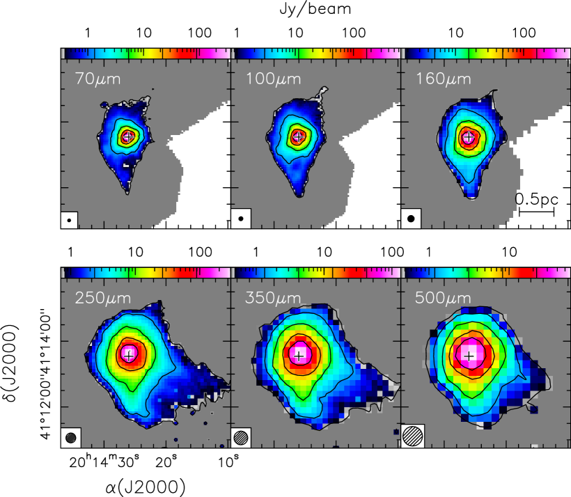
Figure 1: Maps of the IRAS 20126+4104 region obtained with Herschel at different wavelengths, as indicated in each panel. The cross marks the position of the circumstellar disk. The circles in the bottom left denote the full-width at half power of the instrumental beam. The values of the contour levels are marked by vertical bars in the corresponding colour scale.

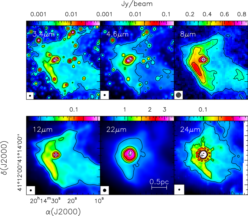
Figure 2: Same as Fig. 1, but for archival images in the IR. The images at 3.4, 4.6, 12, and 22 $\mu$m are from the WISE survey, while those at 8 $\mu$m and 24 $\mu$m are from the MSX survey and the Spitzer database, respectively. The latter image is heavily saturated and shows the pattern of the point spread function of the telescope.

3 Results

3.1 Continuum

The maps of the continuum emission obtained at the six observed bands (70, 100, 160, 250, 350, and 500 $\mu$m) are shown in Fig. 1. In all cases, a clear intensity peak is visible at the position of the circumstellar disk, marked by a cross in the figure. While at the shortest wavelengths, the emission is quite compact; in the sub-millimetre regime, one can see an extension to the south-west, likely associated with colder dust.

For the sake of completeness, we have also retrieved archival IR images at shorter wavelengths of the same region mapped with Herschel. These are shown in Fig. 2. More precisely, we have used data from the Midcourse Space Experiment (MSX) (Price et al. price (1999)), the Wide-field Infrared Survey Explorer (WISE) (Wright et al. wright (2010)), and the Spitzer Space Telescope database (Werner et al. werner (2004); Fazio et al. fazio (2004); Rieke et al. rieke (2004)) Unlike the maps of Fig. 1, the structure of the source appears less concentrated and, in particular, an elongated region of emission is seen to the south-east, probably due to a photo-dissociation region (PDR), as indicated especially by the MSX image at 8 $\mu$m, a wavelength at which PAH emission is very prominent (see, e.g. Tielens tiel (2008)).

All in all, the continuum emission from IRAS 20126+4104 is relatively simple and appears to be dominated by one or more sources concentrated in the central region of a parsec-scale molecular, dusty clump. We can thus derive a reliable estimate of the luminosity of IRAS 20126+4104, as done in the following (see Sect. 4.1).

3.2 Line

As detailed in Sect. 2, the chosen spectral setup allowed us to cover all carbon monoxide rotational transitions from (4–3) to (13–12) as well as the ¹²CO(18–17) and (24–23) lines. At the same time, we observed the oxygen ${}^{3}P_{1}$–${}^{3}P_{2}$ and ${}^{3}P_{0}$–${}^{3}P_{1}$ transitions at 63.18 $\mu$m and 145.53 $\mu$m, respectively, and the $[$Cii$]$ ${}^{2}P_{3/2}$–${}^{2}P_{1/2}$ transition at 157.74 $\mu$m. We also detected the water $2_{2,1}$–$1_{1,0}$ line at 108.07 $\mu$m, which happens to fall in the same band as the ¹²CO(24–23) transition. Unfortunately, in all cases the spectral resolution is largely insufficient to resolve the line profiles and obtain information on the kinematics of the gas. Therefore, in our study we consider only the emission averaged over the lines, whose maps are shown in Figs. 3 and 4.

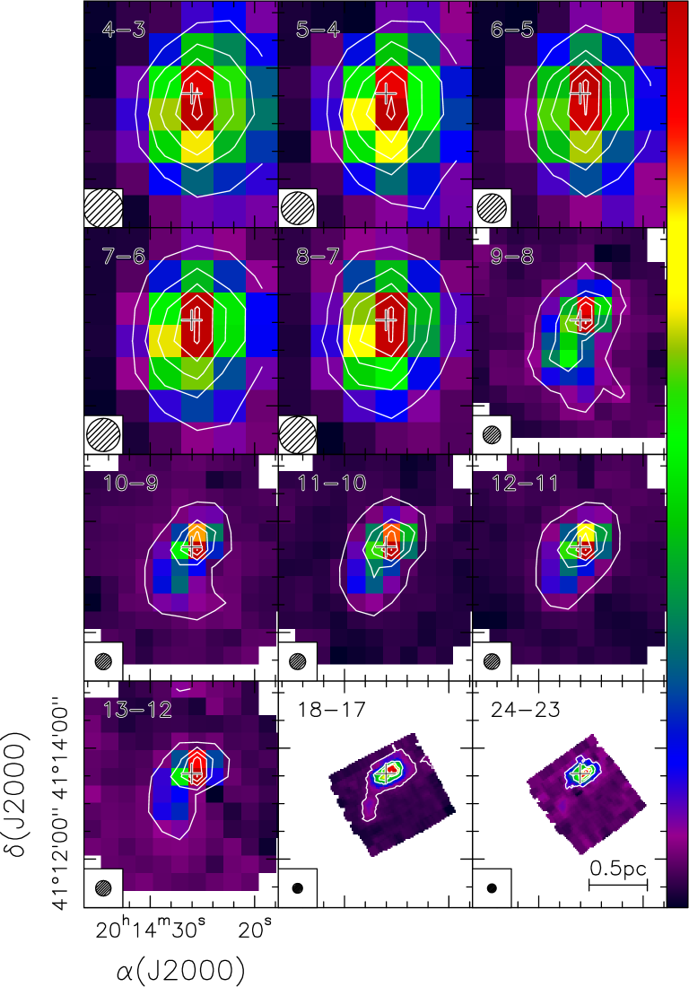
Figure 3: Maps of the emission averaged over the observed ¹²CO lines. The numbers in the top left of each panel indicate the $J+1\rightarrow J$ rotational transition, while the circle in the bottom left denotes the corresponding HPBW. The cross marks the position of the disk. The minimum, maximum, and step for contour levels in units of Jy/beam are as follows (panel by panel, from top to bottom, and from left to right): 3, 15.99, 3.25; 3, 19.63, 4.16; 3, 19.58, 4.14; 3, 25.79, 5.7; 3, 26.51, 5.88; 0.6, 15.98, 3.85; 0.6, 22.89, 5.57; 0.6, 21.25, 5.16; 0.6, 21.42, 5.2; 0.6, 16.99, 4.1; 0.39, 14.13, 3.43; 0.24, 3.69, 0.86.

The most striking difference between the molecular (¹²CO and H₂O) and atomic (Oi and Cii) lines is that the former are basically concentrated around the position of the disk, whereas the latter appear to trace the south-eastern edge of the surrounding parsec-scale clump. We note that the spectral resolution of our observations is not sufficient to resolve the CO line wings and thus it cannot image the outflow lobes previously identified by Shepherd et al. (shep (2000)) and Lebrón et al. (lebr (2006)). Our maps basically trace the bulk emission close to the systemic velocity, which is likely to dominate over the wing emission even in the high energy transitions – as suggested by the ¹²CO(7–6) spectrum of Kawamura et al. (kawa99 (1999)). The same conclusion might hold for the H₂O emission: although no bipolar structure in seen in the corresponding map of Fig. 4, one cannot rule out the possibility that part of the emission arises from the outflow, as found in low-mass protostars (van Dishoeck et al. vandish (2021)).

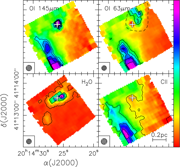
Figure 4: Same as Fig. 3, but for the H₂O, Oi, and Cii lines. The dashed polygon outlines the region where an artefact is present in the Oi 63 $\mu$m line emission. The minimum, maximum, and step for contour levels in units of Jy/beam are as follows (panel by panel, from top to bottom, and from left to right): 1.44, 2.27, 0.21; 13.87, 29.01, 3.78; 0.32, 9.27, 2.24; 32.27, 87.41, 13.78.

In contrast to ¹²CO and H₂O, the atomic lines could arise from the PDR at the border of the clump (see Sect. 3.1) or the shocked region along the southern lobe of the molecular outflow from IRAS 20126+4104. To shed light on the nature of the atomic emission, in Fig. 5 we overlay the Oi 63 $\mu$m map on those of the H₂ 2.12 $\mu$m (from Cesaroni et al. cesa05 (2005)) and Cii lines. Two facts are noteworthy. The first is that the peak of the Oi emission does not coincide with that of the Cii emission. The second is that, in contrast, the distribution of the Oi emission matches that of the H₂ knots well. Although Cii can also be excited in shocks and not only in PDRs (Kristensen et al.  krist13 (2013); Benz et al. benz16 (2016)), these two lines of evidence indicate that in the case of IRAS 20126+4104 the Oi line is in all likelihood associated with shocks in the outflow/jet, while most of the Cii emission traces a PDR. Finally, it is worth noting that unresolved Oi emission is also seen towards the disk position (see Fig. 4), although only in the 145 $\mu$m line (the 63 $\mu$m is affected by an artefact at that position), which is consistent with an analogous detection in disks around low-mass protostars (see e.g. Fedele et al. fed13 (2013)).

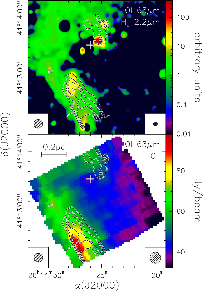
Figure 5: Contour map of the Oi 63 $\mu$m line overlaid on the H₂ 2.12 $\mu$m line image from Cesaroni et al. (cesa05 (2005)) (top panel) and the Cii line map (bottom panel). The circles in the bottom left are the HPBW of the Oi map, while those in the bottom right are the HPBWs of the other lines. Contour levels range from 13.87 to 29.01 in steps of 3.78 Jy/beam.

4 Analysis and discussion

4.1 Luminosity

A reliable estimate of the luminosity of a YSO relies on the availability of high-quality images of the continuum emission at far-IR wavelengths, where the spectral energy distribution (SED) of these objects peaks. In particular, the angular resolution must be good enough to distinguish the emission associated with the YSO from that possibly arising from unrelated nearby objects. As illustrated in Sect. 3.1, our Herschel maps do indeed resolve the region around IRAS 20126+4104 into two components, one being quite compact and peaking at the disk position and the other being more diffuse and approximately coincident with the PDR to the south-east. We constructed the SED of the YSO(s) in IRAS 20126+4104 by considering only the contribution of the compact component. For this purpose, we also used archival data and values from the literature, ranging from the radio to the near-IR domain. In Table 1 we give the flux densities measured at the different bands with references, and in Fig. 6 we plot the corresponding SED. In most cases, the flux densities were taken from catalogues (e.g. IRAS PSC), when available, or from the literature; otherwise, the flux was estimated from the images directly.

Table 1: Total flux densities of the continuum emission from IRAS 20126+4104.

$\lambda$	$\nu$	$S_{\nu}$	Reference
($\mu$m)	(GHz)	(Jy)
3.4	88173.5	0.328	WISE source catalogue
3.6	83275.7	0.79	Johnston et al. (johns (2011))
4.5	66620.5	2.1	Johnston et al. (johns (2011))
5.8	51688.4	1.9	Johnston et al. (johns (2011))
4.6	65171.7	5.704	WISE source catalogue
8.0	51688.4	1.4	Johnston et al. (johns (2011))
8.3	36206.8	0.9646	MSX catalogue 6
9.0	33310.0	5.578	AKARI PSC
10.0	29979.2	0.32	UKIRT (Cesaroni et al. cesa99 (1999))
12.0	24982.5	1.687	WISE source catalogue
12.0	24982.7	$<$2.546	IRAS PSC
12.1	24715.0	1.0970	MSX catalogue 6
12.5	23983.0	1.89	Gemini North (De Buizer debui (2007))
14.7	20463.5	3.9767	MSX catalogue 6
18.0	16655.0	48.96	AKARI PSC
18.3	16382.0	23.5	Gemini North (De Buizer debui (2007))
20.0	14989.6	30	UKIRT (Cesaroni et al. cesa99 (1999))
21.3	14048.4	44.321	MSX catalogue 6
22.0	13626.8	84.482	WISE source catalogue
24.0	12491.0	$>$65	Spitzer
24.5	12236.0	60	Subaru (de Wit et al. dewit (2009))
25.0	11991.7	108.9	IRAS PSC
60.0	4996.54	1381	IRAS PSC
65.0	4612.15	2358	AKARI (from image)
70.0	4283.00	2037	Herschel (this work)
90.0	3331.00	2057	AKARI (from image)
100.0	2997.92	1947	IRAS PSC
100.0	2998.00	2320	Herschel (this work)
140.0	2141.36	1848	AKARI (from image)
160.0	1873.69	1735	Herschel (this work)
160.0	1873.69	1840	AKARI (from image)
250.0	1199.00	859	Herschel (this work)
350.0	856.55	292	JCMT (Cesaroni et al. cesa99 (1999))
350.2	856.00	329	Herschel (this work)
352.9	849.40	477	CSO (Shinnaga et al. shinn (2008))
450.0	666.20	162	JCMT (Cesaroni et al. cesa99 (1999))
455.4	658.30	137	CSO (Shinnaga et al. shinn (2008))
500.5	599.00	123	Herschel (this work)
750.0	399.72	25	JCMT (Cesaroni et al. cesa99 (1999))
850.0	352.70	19	JCMT (Cesaroni et al. cesa99 (1999))
1249.1	240.00	5.8	IRAM (Beuther et al. beu02a (2002))

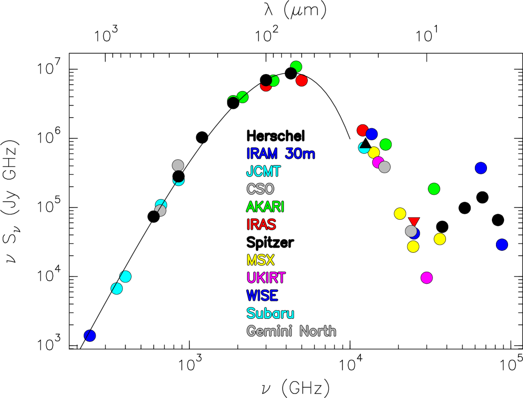
Figure 6: Spectral energy distribution of IRAS 20126+4104 obtained from the data in Table 1. Triangles indicate lower and upper limits. The solid curve is the best fit to the spectrum above 40 $\mu$m obtained with the model described in Sect. 4.3.

As one can see from Fig. 6, the bolometric luminosity is clearly dominated by the emission around 100 $\mu$m and can be estimated by integrating the emission under the SED. For this purpose we have linearly interpolated the flux densities in the $\mbox{\rm log${}_{10}$}\,S_{\nu}$–$\mbox{\rm log${}_{10}$}\,\nu$ plot and obtained $L_{\rm bol}\simeq 1.1\times 10^{4}$ $L_{\odot}$. Now that a precise estimate of the luminosity is available, one may wonder if such a luminosity is dominated by a single massive star or if it contains a significant contribution from other nearby stars. In particular, it is of interest to establish if there is a single star or a binary system at the centre of the disk. Since the mass needed to reproduce the Keplerian pattern of the circumstellar disk is 12 $M_{\odot}$ (see Chen et al. chen (2019)), in Fig. 7, we have plotted the total luminosity of a binary system of total mass 12 $M_{\odot}$, as a function of the mass of the primary member. This was computed for both two zero-age main-sequence (ZAMS) stars and two protostars. For the latter, we referred to Hosokawa et al. (hoso09 (2009)), who demonstrate that the protostellar luminosity up to $\sim$10 $M_{\odot}$ is dominated by the accretion luminosity, whose approximate expression can be obtained from their Eqs. (7) and (13), with the latter having originally been derived by Stahler et al. (sps86 (1986)).

The solid curve in the figure clearly shows that the total luminosity of two ZAMS stars drops dramatically as soon as the mass of the primary decreases from the maximum value of 12 $M_{\odot}$. In fact, even in concentrating the whole mass in a single star, one can obtain only $\sim$80% of the measured bolometric luminosity. The remaining 20% could be made up of nearby lower-mass stars. In fact, according to the simulation described by Sánchez-Monge et al. (sanch (2013)), the most massive member of a stellar cluster emitting $1.1\times 10^{4}$ $L_{\odot}$is expected to be just a $\sim$12 $M_{\odot}$ star.

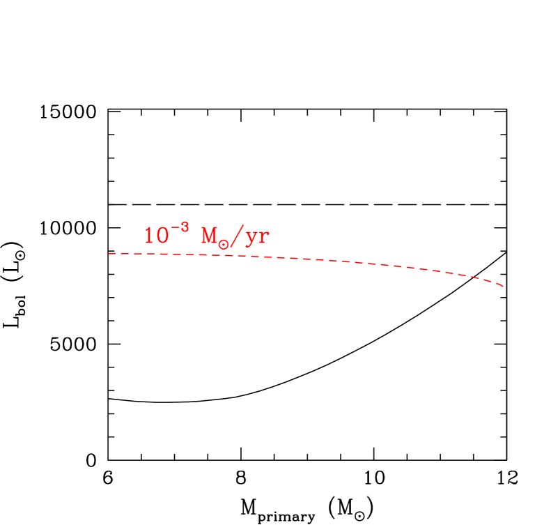
Figure 7: Luminosity of a binary system with a total mass of 12 $M_{\odot}$versus the mass of the primary member. The solid line corresponds to two ZAMS stars. The red dashed curve is for two protostars deriving their luminosity from accretion, for an accretion rate of $10^{-3}\leavevmode\nobreak\ M_{\odot}$ yr^-1. The long-dashed horizontal line marks the bolometric luminosity of IRAS 20126+4104.

In contrast, if the two components of the binary system are protostars, for a fiducial accretion rate of $10^{-3}\leavevmode\nobreak\ M_{\odot}$ yr^-1 (see Cesaroni et al. cesa99 (1999)), the total luminosity is represented by the red dashed line in Fig. 7, which is rather insensitive to the way the mass is partitioned between the primary and the secondary. In this case it seems impossible to decide whether the mass of the system is mostly concentrated in one of the members or more equally shared between them. However, we note that the value of $10^{-3}\leavevmode\nobreak\ M_{\odot}$ yr^-1 is in all likelihood the infall rate through the envelope enshrouding the embedded (proto)star and not the accretion rate through the disk, and hence it must be considered as an upper limit. Indeed, detailed model fits to the SED (Johnston et al. johns (2011)) and line emission (Chen et al. chen (2019)) derive disk accretion rates $\la 10^{-4}\leavevmode\nobreak\ M_{\odot}$ yr^-1. These models prove that the luminosity of IRAS 20126+4104 could originate from a $\sim$12 $M_{\odot}$ ZAMS star with a non-negligible contribution from residual accretion, which is also our conclusion. It is also worth noting that the difference between the infall and accretion rates, that is $\la$$10^{-3}\leavevmode\nobreak\ M_{\odot}$ yr^-1, could correspond to the material ejected into the outflow. Indeed, the estimates of the outflow mass-loss rate in IRAS 20126+4104 range from $8\times 10^{-4}\leavevmode\nobreak\ M_{\odot}$ yr^-1 (Shepherd et al. shep (2000)) to $1.6\times 10^{-2}\leavevmode\nobreak\ M_{\odot}$ yr^-1 (Cesaroni et al. cesa97 (1997)), which correspond to ejection rates an order of magnitude lower for the internal jet entraining the outflow (see e.g. Beuther et al. beu02b (2002)). This implies ejection rates of about $10^{-4}$–$10^{-3}\leavevmode\nobreak\ M_{\odot}$ yr^-1, which is consistent with the difference between infall and accretion rates.

4.2 Temperature and density structure

4.2.1 Derivation from continuum emission

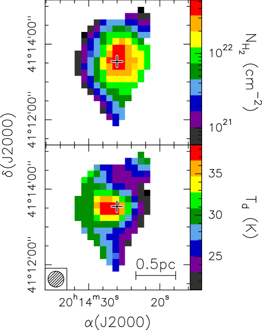
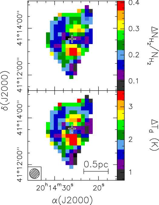
Figure 8: Maps of the gas column density and dust temperature, assuming $\beta=1.5$ (left) and corresponding errors (right). The angular resolution is represented by the circle in the bottom left. The cross marks the position of the circumstellar disk.

Since we have obtained maps of the IRAS 20126+4104 clump at six wavelengths across the peak of the SED, we could derive a temperature and column density estimate all over these maps by fitting the Herschel fluxes. In practice, we decided to ignore the 500 $\mu$m maps, whose HPBW ($\sim$36″) is the largest, and thus achieved a compromise between the quality of the fit and angular resolution. All maps were smoothed to the angular resolution of the 350 $\mu$m map, that is 25″, and resampled on the same grid. Then a SED was extracted for each pixel, rejecting the SEDs with one or more fluxes lying below the corresponding 3$\sigma$ level. Finally, by means of command MFIT of GILDAS, we fitted the SEDs with a modified black body using the expression

$$S_{\nu}=\Omega_{\rm B}\,B_{\nu}(T)\left(1-{\rm e}^{-\tau}\right),$$ (1)

where $B_{\nu}$ is the Planck function, $\Omega_{\rm B}$ the solid angle of the beam, $T$ the dust temperature, and $\tau$ the dust opacity. Moreover,

$$\tau=\kappa_{0}\left(\frac{\nu}{\nu_{0}}\right)^{\beta}\frac{\mu m_{\rm H}}{\mathcal{R}}N,$$ (2)

with $\kappa_{0}$ the dust absorption coefficient at frequency $\nu_{0}$, $\mu$ the mean molecular weight, $m_{\rm H}$ the mass of the hydrogen atom, $\mathcal{R}$ the gas-to-dust mass ratio, and $N$ the column density along the line of sight. For our calculation we adopted the values $\kappa_{0}=1$ cm² g^-1, $\nu_{0}=230$ GHz, and $\mu=2.8$, $\mathcal{R}=100$.

The free parameters of the fit are the dust temperature and column density, while $\beta$ is assumed equal to the value of 1.5, obtained by fitting the global SED in Fig. 6 above 40 $\mu$m with Eq. (1), where $\Omega_{\rm B}$ is replaced by the solid angle subtended by the whole clump, $\Omega_{\rm c}=\pi\theta^{2}$, with $\theta\simeq 70\arcsec$ (see Fig. 1). The same fit also provides us with an estimate for the mass and temperature of the clump 150 $M_{\odot}$ and 33 K, respectively (but see Sect. 4.3).

In Fig. 8 we show the resulting maps and the corresponding errors. As expected, the column density and temperature peak approximately at the position of the disk, within the angular resolution of the images. The column density map allowed us to derive a more precise estimate of the clump mass, as done later in Sect. 4.3.

All the above holds for the cold-dust component, but it is also interesting to explore the temperature distribution of the hot-dust component contributing to the continuum emission below $\sim$40 $\mu$m. This can be seen in a map of the colour temperature obtained from the WISE 22 and 12 $\mu$m images, after smoothing to the same angular resolution. The result is shown in Fig. 9, where we have also overlaid the temperature map of the cold-dust component (from Fig. 8), for the sake of comparison. Clearly, the dust temperature peaks where the colour temperature experiences a dip, which is consistent with most of the near-IR emission being confined to the surface of the clump.

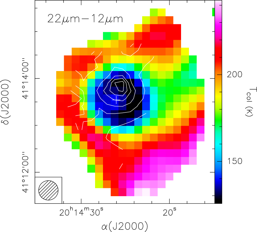
Figure 9: Map of the dust temperature from Fig. 8 overlaid on the map of the colour temperature obtained from the WISE 12 and 22 $\mu$m images. The angular resolution is denoted by the circle in the bottom left.

4.2.2 Derivation from ¹²CO emission

Another description of the temperature and density distribution in the clump enshrouding IRAS 20126+4104 could be obtained from the ¹²CO emission. In Fig. 10, we show the rotation diagram obtained from the ¹²CO emission integrated over the line and the whole emitting area, whose angular size is $\sim$150″ (see Fig. 3). One can see that the points are not distributed along a straight line, which is expected if the source were isothermal and homogeneous. This is not surprising because we know from our analysis in Sect 4.2.1 that the temperature varies over the clump. To fit the rotation diagram, one thus needs a model that takes temperature and, possibly, density gradients into account. For this purpose, we referred to the approach adopted by Mauersberger et al. (mau88 (1988); hereafter MWH – see their appendix) and Neufeld (neuf12 (2012)). Our derivation of the mean column density, $N_{J}$, in a rotational level of ¹²CO is slightly different from that of those authors and is described in Appendix A. In practice, we express $N_{J}$ as a function of the energy of the level, $E_{J}$, through a number of variables that are all known, except the temperature at the surface of the clump, $T_{\rm o}$, the mean column density of ¹²CO, $N_{\rm CO}$, and the index $\alpha=(q-p-3)/q$, where $q$ and $p$ are the power-law exponents of the temperature and density profiles, respectively.

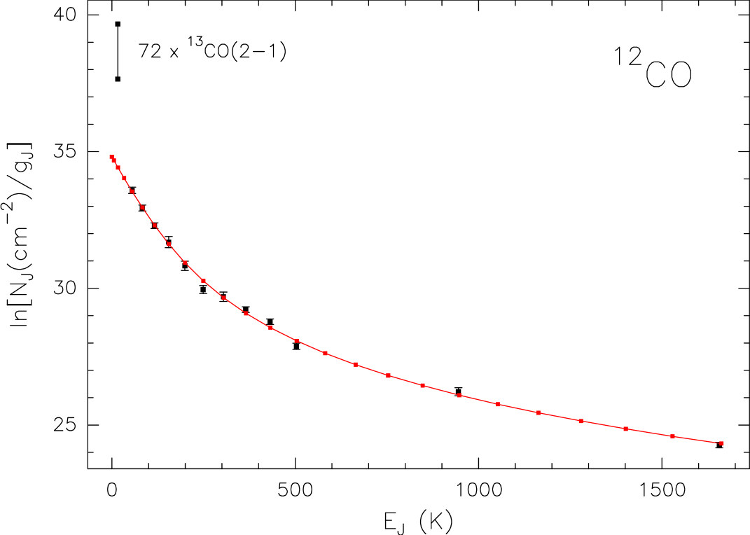
Figure 10: Rotation diagram of ¹²CO. The black points with error bars represent the Herschel data, whereas the two black points connected by a bar are the lower and upper limit to the ¹³CO column density in the $J=2$ level obtained from the ¹³CO(2–1) data of Cesaroni et al. (cfw99 (1999)) after multiplying the column density for a ¹²CO/¹³CO abundance ratio of 72. The red points connected by the curve are the best fit to the Herschel data obtained with the model described in Appendix A.

The best fit to the rotation diagram is shown by the red curve in Fig. 10 and corresponds to the minimum $\chi^{2}$ obtained by varying the three free parameters over suitable ranges. We thus obtain $T_{\rm o}=32\pm 5$ K, $N_{\rm CO}=(2.2^{+1.8}_{-1.0})\times 10^{16}$cm^-2, and $\alpha=3.15\pm 0.13$. We note that all the above assumes local thermodynamic equilibrium (LTE) and optically thin ¹²CO lines. To verify if these assumptions are valid, we ran the programme RADEX by Van der Tak et al. (vdtak (2007)) using – as inputs – the column density obtained from the fit in Fig. 10, a temperature and H₂ density spanning the ranges 30–200 K and $10^{3}$–$10^{6}$ cm^-3, respectively, and a line width of 8 km s^-1 (see Fig. 1 of Kawamura et al. kawa99 (1999)). The results confirm that all lines are optically thin, with the highest value of the opacity, 0.3, being obtained for the ¹²CO(4–3) transition. We conclude that our approach is plausible and self-consistent.

The mass of the clump, obtained from Eq. (16), is $M_{\rm H_{2}}\simeq 5.5^{+4.6}_{-2.5}\leavevmode\nobreak\ M_{\odot}$ for an abundance of ¹²CO relative to H₂ of $10^{-4}$. The value of $M_{\rm H_{2}}$ is by far too small compared to other estimates such as that obtained from the continuum emission (see Sect. 4.2.1) or the one derived by Shepherd et al. (shep (2000)) from their ¹²CO and ¹³CO (1–0) interferometric maps ($\sim$300 $M_{\odot}$). Such a discrepancy indicates that most of the material must be cold enough to be traced only by the low-energy lines of ¹²CO and its isotopologues. To include the contribution of these lines in the rotation diagram, we have used the single-dish ¹³CO(2–1) data of Cesaroni et al. (cfw99 (1999)). These authors mapped only a limited portion of the whole clump, about 48″$\times$48″ centred around the peak of the emission. Therefore, we could derive an upper limit of $1.17\times 10^{16}$ cm^-2 to the mean column density over $\Omega_{\rm c}$ in the $J=2$ level of ¹³CO, by assuming that the part of the clump that was not mapped in ¹³CO(2–1) has the same mean column density as the mapped one. Conversely, a lower limit of $1.56\times 10^{15}$ cm^-2 was obtained by assuming that no ¹³CO emission is present beyond the region mapped by Cesaroni et al. (cfw99 (1999)).

In Fig. 10, we have plotted the corresponding lower and upper limits on the ¹²CO column density obtained by multiplying the ¹³CO values by a ratio between the ¹²CO and ¹³CO abundances of 72, estimated from Wilson & Rood (wilroo (1994)) for a galactocentric distance of 8.2 kpc. From the rotation diagram of the (2–1) and (4–3) lines only, one obtains a temperature and ¹²CO column density in the range 6.4–9.6 K and $4.2\times 10^{17}$–$4.8\times 10^{18}$ cm^-2, respectively. The latter corresponds to $M_{\rm H_{2}}$=90–1050 $M_{\odot}$, a range consistent with the estimates obtained in other tracers. This confirms that the majority of the clump is sufficently cold to be seen only in the low-energy transitions of the CO isotopologues.

Despite their limited utility in sampling the cold outer region of the clump, where most of the mass is concentrated, the high-energy transitions of ¹²CO still provide us with important information on the innermost structure of the clump. In Sect. 4.2.2, we have derived $\alpha=(q-p-3)/q\simeq 3.15$. It is also known that $q$ is related to the spectral index $\beta$ of the optically thin (sub-)millimetre continuum emission by the relation $q=-2/(4+\beta)$ (see e.g. Doty & Leung dole (1994)). Since in our case $\beta\simeq 1.5$ (see Sect. 4.2.1), we obtain $q\simeq-0.37$ and, consequently, $p\simeq-2.2$, which proves that the density distribution inside the clump is steeply peaked towards the centre. In all likelihood, this indicates that the envelope enshrouding IRAS 20126+4104 is currently collapsing and accreting onto the disk.

4.3 Mass of the clump

The results obtained so far can be used to derive an accurate estimate of the clump mass. We have already mentioned in Sect. 4.2.1 that a mass estimate can be obtained from a fit to the (sub-)millimetre and far-IR part of the SED, using a modified black body that assumes the clump to be isothermal and homogeneous. The best fit provides us with a mass of 150 $M_{\odot}$ and a temperature of 33 K. However, as demonstrated in Sect. 4.2, there are significant temperature and density variations around IRAS 20126+4104, so that a more realistic model is needed to improve upon these estimates.

An estimate taking such temperature and density variations into account can be directly obtained from the map in Fig. 8, by integrating the column density over the whole clump:

$$M_{\rm c}=\mu m_{\rm H}\sum_{i}N_{i}\leavevmode\nobreak\ \Delta\Omega\,d^{2},$$ (3)

where $i$ indicates a pixel of the column density map in Fig. 8, $N_{i}$ is the gas column density at pixel $i$, $\Delta\Omega=100$ arcsec² is the pixel’s solid angle, the sum extends over all pixels where the column density has been estimated, $d$=1.64 kpc is the distance of IRAS 20126+4104, and the other symbols have the same meaning as in Eq. (2). We calculated a total mass of 245 $M_{\odot}$, which is significantly greater than the 150 $M_{\odot}$ estimated from the modified black-body fit.

Another way to derive $M_{\rm c}$ is to fit the (sub-)millimetre and far-IR part of the SED with the model by Cesaroni (rcesa19 (2019)), which takes both temperature and density gradients into account in the form of power laws. For the dust absorption coefficient, we used the same value adopted for Eq. (2), with $\beta=1.5$. The input parameters of the model are the radius of the clump, $R_{\rm o}$, the ratio between the inner and outer radius, $R_{\rm i}/R_{\rm o}$, the distance to the source, $d$, the power-law indices of the temperature, $q$, and density, $p$, the temperature at the outer radius, $T_{\rm o}$, and the mass of the clump, $M_{\rm c}$. From Sect. 4.2.2, we know that $q=-0.37$ and $p=-2.2$, while from the maps in Fig. 1 we measured an angular radius of the clump of $\sim$70″, which implies $R_{\rm o}=0.56$ pc for $d=1.64$ kpc. The minimum radius, $R_{\rm i}$, beyond which the spherically symmetric approximation holds can be assumed to be the centrifugal radius of the disk. The latter was estimated to be a few $\sim$1000 au, depending on the model (Keto & Zhang ketzha (2010); Johnston et al. johns (2011); Chen et al. chen (2019)). Therefore, for our model fit, we assume $R_{\rm i}/R_{\rm o}=0.05$.

The best fit to the SED for $\lambda>40$ $\mu$m was obtained by varying $M_{\rm c}$ and $T_{\rm o}$ over suitable ranges. In Fig. 11, we have plotted the value of $\chi^{2}$ as a function of these two variables, with the contour corresponding to a confidence level of 1$\sigma$, according to the criterion of Lampton et al. (lamp (1976)). In this calculation, we have assumed an error of 20% for all fluxes. We conclude that $T_{\rm o}=18^{+1.8}_{-1.5}$ K and $M_{\rm c}=220^{+85}_{-60}$ $M_{\odot}$. The latter value is in agreement with that obtained by integrating the column density over the region, while the surface temperature of the clump is comparable to the minimum value (21 K) of the temperature map in Fig. 8. We note that this value of the temperature is very similar to that expected at a distance $R_{\rm o}=0.56$ pc from a star of $L_{\ast}=1.1\times 10^{4}$ $L_{\odot}$. In fact, following Zhang et al. (zha02 (2002)), one obtains

$$T_{\rm o}=65\left(\frac{0.1{\rm pc}}{R_{\rm o}}\right)^{\frac{2}{4+\beta}}\left(1.25\frac{L_{\ast}}{10^{5}\leavevmode\nobreak\ \mbox{$L_{\odot}$}}\right)^{\frac{1}{4+\beta}}\simeq 24\leavevmode\nobreak\ K,$$ (4)

with $\beta=1.5$ (see Sect. 4.2.1).

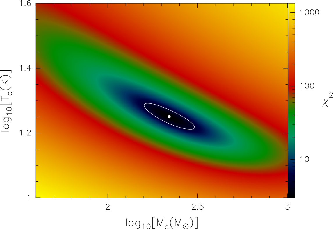
Figure 11: Plot of the $\chi^{2}$ obtained by fitting the clump model of Cesaroni (rcesa19 (2019)) to the SED of IRAS 20126+4104 (shown in Fig. 6), as a function of the clump surface temperature and mass. For the $\chi^{2}$ calculation, we have assumed an error of 20% for all fluxes. The white dot marks the minimum corresponding to the best fit, while the white contour is the 1$\sigma$ confidence level (i.e. 68% reliability) according to the criterion of Lampton et al. (lamp (1976)).

We conclude that our analysis indicates that the clump enshrouding IRAS 20126+4104 has a mass of $\sim$250 $M_{\odot}$ with a density distribution $\propto R^{-2.2}$, while the temperature is relatively low, $\sim$20 K, at the surface of the clump and increases as $R^{-0.37}$ towards the centre.

4.4 Shocked region

As noted in Sect. 3.2, the oxygen line emission very likely originates from shocked gas, given the positional coincidence with H₂ knots in the jet from IRAS 20126+4104. Under this hypothesis, one can derive an estimate of the oxygen column density, $N_{\rm O}$, and H₂ volume density, $n_{\rm H_{2}}$, from the two Oi lines observed. For our calculations we used the programme RADEX (Van der Tak et al. vdtak (2007)) with the oxygen atomic data from Schöier et al. (shoier (2005)), assuming collisions only with H₂ molecules, a kinetic temperature of 500 K, and a line width of 20 km s^-1, a fiducial value suggested by observations of the oxygen line in other objects (Kristensen et al. krist17 (2017); Yang et al. yang22 (2022)). The results are weakly dependent on the temperature (see also Fig. 10 of Nisini et al. nisi (2015)) and line width; therefore, our choice cannot significantly affect the outcome of RADEX. We also note that if we were to choose collisions with H instead of H₂, no solution would be found for $N_{\rm O}$ or $n_{\rm H_{2}}$(see below).

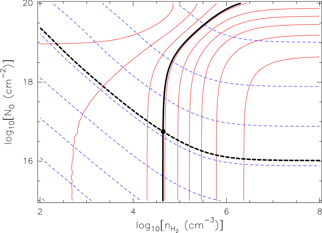
Figure 12: Example of the method used to estimate the oxygen column density and the molecular hydrogen volume density over the Oi-emitting region. The solid red contours and the blue dashed contours are maps of $\int T_{\rm 63\mu m}{\rm d}V/\int T_{\rm 145\mu m}{\rm d}V$ and $\int T_{\rm 63\mu m}{\rm d}V$, respectively. The solid, thick black contour and the black dashed contour correspond to the observed values of the same quantities. The dot marks the intersection between these two contours, which gives the pair of values of $n_{\rm H_{2}}$ and $N_{\rm O}$ ($4.4\times 10^{4}$ cm^-3 and $5.6\times 10^{16}$ cm^-2) that reproduce both observables.

We searched for the pair of values $N_{\rm O}$,$n_{\rm H_{2}}$ that can reproduce both the ratio between the 63 and 145 $\mu$m lines and the value of the 63 $\mu$m line intensity. For this purpose, we computed the ratio between the maps of the integrated emission in these two lines, after suitably resampling and smoothing to the same resolution. Then, at each pixel, we extracted the value of the line ratio and that of the 63 $\mu$m brightness temperature integrated over the line. These were used to derive $N_{\rm O}$ and $n_{\rm H_{2}}$ as illustrated in Fig. 12. In practice, we computed a grid of line intensities (in K km s^-1) for a wide range of $N_{\rm O}$ and $n_{\rm H_{2}}$ and then in the plane $n_{\rm H_{2}}$,$N_{\rm O}$ we plotted the contour levels corresponding to the observed values of $\int T_{\rm 63\mu m}{\rm d}V$ and $\int T_{\rm 63\mu m}{\rm d}V/\int T_{\rm 145\mu m}{\rm d}V$. The intersection between the two contours gives the pair $n_{\rm H_{2}}$,$N_{\rm O}$ , satisfying both conditions. As previously mentioned, if collisions with only atomic hydrogen are included, the two contours do not intersect and no solution is found.

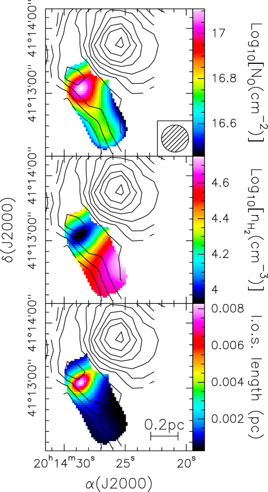
Figure 13: Maps of the oxygen column density (top panel) and molecular hydrogen volume density (middle panel) over the shocked region where Oi emission is detected. The bottom panel shows a map of the geometrical thickness along the line of sight of the same region, derived from the ratio between $N_{\rm O}$ and $n_{\rm H_{2}}$, assuming a constant oxygen abundance relative to molecular hydrogen of $6\times 10^{-4}$. The contours represent the same map of the gas column density as in Fig. 8.

After applying this procedure to each pixel of the maps, we obtained the distribution of $N_{\rm O}$ and $n_{\rm H_{2}}$ along the shocked region to the south-east of the clump, where the southern lobe of the (precessing) jet from IRAS 20126+4104 is seen. The results are shown in Fig. 13, where also a contour map of the gas column density from Fig. 8 has been overlaid for the sake of comparison.

From the ratio between $N_{\rm O}$ and $n_{\rm H_{2}}$ , one can obtain an estimate of the thickness of the oxygen-emitting region along the line of sight. For this purpose, we have assumed an abundance of oxygen with respect to H equal to the typical interstellar-medium value of $3\times 10^{-4}$ (Savage & Sembach savsem (1996)), which implies an abundance relative to H₂ of $6\times 10^{-4}$. The resulting map is shown in the bottom panel of Fig. 13. The result depends on the oxygen abundance, which could be an order of magnitude lower than the value adopted by us (see e.g. Liseau & Justtanont lis09 (2019)). However, even if the abundance were overestimated by a factor $\sim$10, the geometrical thickness of the shocked region would be much less than the size of the same region in the plane of the sky. This suggests that we are looking at the shocked layer approximately face on.

All the previous results favour an origin of the Oi remission from dissociative shocks in the southern lobe of the jet powered by IRAS 20126+4104. With this in mind, we used Eq. (7) of Hollenbach (holl (1985)) to derive the mass-loss rate in the jet, $\dot{M}_{\rm o}$, from the luminosity of the Oi 63 $\mu$m line. This equation can be used provided the density of the shocked region and the shock velocity satisfy the condition $\mbox{$n_{\rm H_{2}}$}\,\varv_{\rm sh}\la 10^{12}$ cm^-2 s^-1. In our case, $\mbox{$n_{\rm H_{2}}$}<5\times 10^{4}$ cm^-3, as shown in Fig. 13, and $\varv_{\rm sh}\la 100$ km s^-1, which was obtained from proper motion measurements of the H₂O masers (Moscadelli et al. mosca05 (2005, 2011)) and H₂ knots (Massi et al. massi23 (2023)). Therefore, $\mbox{$n_{\rm H_{2}}$}\,\varv_{\rm sh}<5\times 10^{11}$cm^-2 s^-1, which satisfies the previous condition.

The 63 $\mu$m line luminosity was obtained by integrating over the whole emitting region and has turned out to be $\sim$2 $L_{\odot}$, which implies $\dot{M}_{\rm o}\simeq 4\times 10^{-4}$ $M_{\odot}$ yr^-1, where the result has been multiplied by a factor 2 to take into account the fact that we have analysed only one of the two lobes of the outflow. This value is consistent within the uncertainties with that of $8\times 10^{-4}$ $M_{\odot}$ yr^-1 obtained by Shepherd et al. (shep (2000)) from their ¹²CO(1–0) high-resolution map and it is also the mass outflow rate expected for a high-mass YSO of $\sim 1.1\times 10^{4}$ $L_{\odot}$, as one can see in Fig. 4 of López-Sepulcre et al. (lose09 (2009)) and Fig. 5 of Maude et al. (maud15 (2015)). Despite the good agreement between the outflow rates obtained from Oi and ¹²CO, one must keep in mind that the two tracers are not necessarily related for a variety of reasons, which has been extensively discussed by Mottram et al. (mott17 (2017)). In particular, the Oi line is probably associated with the current accretion-ejection episode, whereas the low-J ¹²CO lines are more representative of the time-averaged accretion-ejection phenomenon. One could speculate that the similarity between the two estimates in IRAS 20126+4104 suggests that, in this object, accretion proceeds in a less episodic way than in other sources where significant accretion outbursts have been detected (Caratti o Garatti et al. cagana (2017); Hunter et al. hunt (2017)).

5 Summary and conclusions

Herschel observations of the continuum and line emission from the high-mass (proto)star IRAS 20126+4104 were performed with the main goal of deriving an accurate estimate of the stellar luminosity, clump mass, and outflow mass-loss rate. In particular, we imaged a region of $\sim$1 pc at six continuum bands, in twelve ¹²CO rotational transitions, and three atomic (Oi and Cii) lines. Serendipitously, also an H₂O line was detected.

From the continuum data, we have estimated a bolometric luminosity of $1.1\times 10^{4}$ $L_{\odot}$. We show that in all likelihood, this luminosity is mostly contributed to by a $\sim$12 $M_{\odot}$ ZAMS star at the centre of the Keplerian disk imaged in previous studies.

We have also derived maps of the gas column density and dust temperature. Not surprisingly, both the temperature and column density peak at the positions of the disk. The mass of the clump has been obtained both by integrating the column density over the mapped region and through a model fit to the SED that takes temperature and density gradients into account. We have found that the clump mass is $\sim$250 $M_{\odot}$ with a steep density distribution $\propto R^{-2.2}$, which supports the idea that the envelope enshrouding the disk is infalling.

While the molecular transitions trace the majority of the clump seen in the (sub-)millimetre continuum, the atomic lines are detected only towards the disk and south-eastern border of the clump. However, the peak of the Oi emission is clearly offset from that of the Cii emission, with the former coinciding with the jet knots revealed by the H₂ emission at 2.12 $\mu$m and the latter probably being associated with a PDR seen at near-IR wavelengths. This indicates that the Oi emission most likely originates from shocks. At the same time, one cannot rule out that part of the Cii line emission also comes from shocks, as some Cii emission is seen towards the peak of Oi. From the maps of the two Oi lines, we have determined the distribution of the oxygen column density and H₂ volume density over the shocked border by fitting the data with the RADEX numerical code. Finally, the Oi emission arising from dissociative shocks has been used to derive an estimate of the outflow mass-loss rate, which is $\sim$$4\times 10^{-4}$ $M_{\odot}$ yr^-1. Such a value is indeed expected for a YSO of $1.1\times 10^{4}$ $L_{\odot}$ (López-Sepulcre et al. lose09 (2009); Maude et al. maud15 (2015)).

Appendix A Rotation diagram with temperature and density gradients

We present a model to fit the rotation diagram of a molecule, which takes the presence of temperature and density gradients into account. Our approach is inspired by the modified Boltzmann relation of MWH and Neufeld (neuf12 (2012)), but it differs from their approaches for a number of reasons. The Neufeld method is similar to ours, but it does not take density gradients into account nor does it provide an expression for the CO column density – as we illustrate below with Eq. (15). As for MWH, they assume an infinite clump, whereas we consider a clump of finite radius. More specifically, assuming spherical symmetry and temperature and density laws for the molecule of the type $T\propto R^{q}$ and $n\propto R^{p}$, with $R$ being the distance from the centre, MWH found that the mean column density over the cloud in a level of energy $E$, divided by the statistical weight, is proportional to $E^{-\alpha}$, where $\alpha$ is a function of $q$ and $p$. They concluded that the relationship between column density and energy should be fitted by a straight line in a modified rotation diagram where the logarithms of both quantities are reported (in contrast to the traditional rotation diagram where the linear relationship is expected in a plot of $\log N$ vs $E$). The problem with this approach is that it works only if the level energy is sufficiently high. In particular, it fails to describe the ground state level, where $E=0$ and the expression for the column density diverges. Moreover, the expression obtained by MWH allows derivation of $\alpha$, but it cannot be used to compute the temperature and total column density of the molecule, in contrast with the usual rotation diagrams.

With all the above in mind, we have developed a slightly different model that does not suffer from the above inconveniences. We assume that the molecular clump is a sphere of radius $R_{\rm o}$ with temperature and density given by the following expressions:

$$T = T_{\rm o}\left(\frac{R}{R_{\rm o}}\right)^{q}$$ (5)

$$n = n_{\rm o}\left(\frac{R}{R_{\rm o}}\right)^{p},$$ (6)

with $R$ being the distance from the centre. For a given energy level, $J$, the mean column density over the clump is equal to

$$N_{J} = \frac{4\pi}{\Omega_{\rm c}d^{2}}\int_{0}^{R_{\rm o}}n_{j}R^{2}{\rm d}{R}$$ (7)

$$= \frac{4}{R_{\rm o}^{2}}\int_{0}^{R_{\rm o}}n_{\rm o}\left(\frac{R}{R_{\rm o}}\right)^{p}g_{J}\frac{B}{T}\exp\left(-\frac{E_{J}}{T}\right)R^{2}{\rm d}{R}$$ (8)

$$= 4R_{\rm o}n_{\rm o}g_{J}B\int_{0}^{1}\frac{x^{p}}{T}\exp\left(-\frac{E_{J}}{T}\right)x^{2}{\rm d}{x},$$ (9)

with $x=R/R_{\rm o}$, $d$ the distance to the source, and $\Omega_{\rm c}=\pi R_{\rm o}^{2}/d^{2}$ the solid angle subtended by the clump. The rotational constant, $B$, and $E_{J}$ are both expressed in temperature units. Here we have used Eq. (6) and the Boltzmann law $n_{J}=g_{J}(n/Q)\exp(-E_{J}/T)$ with the $Q(T)$ partition function. We have also assumed $Q=T/B$ for $T\gg B$, an approximation that holds for the ¹²CO molecule (see Townes & Schawlow tosh (2015)). However, a similar calculation can be made as long as $Q\propto T^{\gamma}$ (in the case of MWH, $\gamma=3/2$).

We treated the two cases $J=0$ and $J>0$ separately. For $J=0$, the ground-state energy is $E_{0}=0$ and the previous equation simplifies to

$$\frac{N_{J}}{g_{J}}=4R_{\rm o}n_{\rm o}\frac{B}{T_{\rm o}}\int_{0}^{1}x^{2+p-q}{\rm d}{x}=\frac{4}{(3+p-q)}R_{\rm o}n_{\rm o}\frac{B}{T_{\rm o}}.$$ (10)

For $J>0$, following MWH, we have rewritten the integral expressing $x$ as a function of $y=T/T_{\rm o}$ by means of Eq. (5), where we assume $q<0$:

$$\frac{N_{J}}{g_{J}} = -\frac{4}{q}R_{\rm o}n_{\rm o}\frac{B}{T_{\rm o}}\int_{1}^{\infty}y^{\frac{3+p-2q}{q}}\exp\left(-\frac{E_{J}}{T_{\rm o}y}\right)\,{\rm d}{y}$$ (11)

$$= -\frac{4}{q}R_{\rm o}n_{\rm o}\frac{B}{T_{\rm o}}\left(\frac{E_{J}}{T_{\rm o}}\right)^{-\alpha}\int_{0}^{\frac{E_{J}}{T_{\rm o}}}t^{\alpha-1}\exp(-t)\,{\rm d}{t},$$

where we have defined $t=E_{J}/(T_{\rm o}y)$ and $\alpha=(q-p-3)/q$.

In conclusion, we obtain the following:

$$\frac{N_{J}}{g_{J}}=\left\{\begin{array}[]{lcl}\frac{A}{\alpha\Gamma(\alpha)}&\Leftrightarrow&J=0\\ A\left(\frac{E_{J}}{T_{\rm o}}\right)^{-\alpha}P\left(\alpha,\frac{E_{J}}{T_{\rm o}}\right)&\Leftrightarrow&J>0\\ \end{array}\right.,$$ (12)

where we have defined

$$A=-\frac{4}{q}\Gamma(\alpha)\,R_{\rm o}\,n_{\rm o}\frac{B}{T_{\rm o}},$$ (13)

and

$$P(a,x)=\frac{1}{\Gamma(a)}\int_{0}^{x}t^{a-1}\exp(-t)\,{\rm d}{t}$$ (14)

is the incomplete gamma function. It is worth noting that, in the limit $E_{J}/T_{\rm o}\gg 1$, we have recovered the result of MWH, $N_{J}/g_{J}\propto E_{J}^{-\alpha}$, because $\lim_{E_{J}/T_{\rm o}\to+\infty}{P(\alpha,E_{J}/T_{\rm o})}=1$.

By fitting Eq. (12) to the data in a rotation diagram, one can obtain the parameters $A$, $T_{\rm o}$, and $\alpha$. Finally, one can relate the mean column density of the molecule, $N$, and the mass of the clump, $M_{\rm H_{2}}$, to the values of these three parameters as follows:

$$N = \frac{1}{\Omega_{\rm c}d^{2}}\int_{0}^{R_{\rm o}}n\,4\pi R^{2}{\rm d}{R}$$ (15)

$$= \frac{4}{p+3}n_{\rm o}R_{\rm o}$$

$$= \frac{A}{(\alpha-1)\Gamma(\alpha)}\frac{T_{\rm o}}{B}$$

$$M_{\rm H_{2}} = \mu m_{\rm H}\,\Omega_{\rm c}d^{2}\frac{N}{X},$$ (16)

where $X$ is the abundance of the molecule relative to H₂ and we have used Eq. (13) to express $n_{\rm o}$ as a function of $A$.