On the Interaction between Node Fairness and Edge Privacy
in Graph Neural Networks

Abstract

Due to the emergence of graph neural networks (GNNs) and their widespread implementation in real-world scenarios, the fairness and privacy of GNNs have attracted considerable interest since they are two essential social concerns in the era of building trustworthy GNNs. Existing studies have respectively explored the fairness and privacy of GNNs and exhibited that both fairness and privacy are at the cost of GNN performance. However, the interaction between them is yet to be explored and understood. In this paper, we investigate the interaction between the fairness of a GNN and its privacy for the first time. We empirically identify that edge privacy risks increase when the individual fairness of nodes is improved. Next, we present the intuition behind such a trade-off and employ the influence function and Pearson correlation to measure it theoretically. To take the performance, fairness, and privacy of GNNs into account simultaneously, we propose implementing fairness-aware re-weighting and privacy-aware graph structure perturbation modules in a retraining mechanism. Experimental results demonstrate that our method is effective in implementing GNN fairness with limited performance cost and restricted privacy risks.

1 Introduction

In recent years, in addition to competent performance, there has been an increasing desire for fairness Agarwal et al. (2021); Li et al. (2021); Dong et al. (2021) and private information security Wu et al. (2022a, 2021) in GNNs, because both privacy and fairness are two essential concerns of GNN users Zhang et al. (2022). In the context of GNNs, existing studies He et al. (2021); Kang et al. (2020) only focus on performance and privacy/fairness; however, privacy and fairness are not isolated from each other in practical scenarios. For example, in e-commerce platforms Guo et al. (2022); Zhu et al. (2019), where users and items are considered as nodes and their interactions are regarded as edges in a graph, a recommender system should serve all users with competent performance. Meanwhile, user bias Wu et al. (2022d) should be avoided and similar users (i.e., nodes) should receive similar item recommendations to boost individual fairness; the purchase records of a customer (i.e., edges between nodes) should not be exposed to others without permission. Therefore, it is necessary to study the interaction among performance, fairness, and privacy to build trustworthy GNNs comprehensively Zhang et al. (2022); Sharma et al. (2022).

Existing literature has studied the interaction between performance and fairness/privacy of GNNs. For example, to boost individual fairness in GNNs, a method called REDRESS Dong et al. (2021) proposes to add a regularisation term concerning fairness from the ranking perspective into the loss function of GNNs. Moreover, InFoRM Kang et al. (2020) uses the Lipschitz property and proposes a metric to evaluate the individual fairness of nodes. This metric can also be involved in the loss function of a target model to reduce the bias existing in the GNN predictions. To promote edge privacy, for instance, Wu et al. Wu et al. (2022b) explore the vulnerability of edges in the training graph and introduce differential privacy (DP) mechanisms Sajadmanesh and Gatica-Perez (2021) to protect edges from leakage. These studies also demonstrate that both individual fairness and edge privacy are at cost of GNN performance.

To comprehensively build trustworthy GNNs, it is inevitable to study the interaction between fairness and privacy. Currently, a few works have explored the impact of improving model privacy on fairness Zhang et al. (2021) or promoting algorithm fairness on privacy Chang and Shokri (2021), which are in the context of general machine learning models for Independent Identically Distribution (IID) data. In contrast, this paper will study the interaction of node fairness and edge privacy of GNNs for complex graph data, which has not yet been explored and measured to the best of our knowledge. Moreover, given the trade-off between fairness/privacy and performance and unexplored interaction between fairness and privacy, a challenging research topic of building trustworthy GNNs is how to ensure the privacy and fairness of a GNN model simultaneously with keeping competent model performance (i.e., with limited performance cost).

In this paper, we empirically verify the adverse effect of individual fairness of nodes on edge privacy in GNN models. To understand this observation, we employ the influence functions of training samples to measure and explain this trade-off. Furthermore, we propose a Privacy-aware Perturbations and Fairness-aware Re-weighting (PPFR) method to implement GNN fairness with limited performance cost and restricted privacy risks. The contributions of this paper are summarised as follows:

• In this paper, we explore the interaction between fairness and privacy of GNN for the first time. We empirically show that the edge privacy risk increases when enhancing individual fairness of nodes, i.e., there exists a trade-off between fairness and privacy of GNNs.

• To understand GNN behaviours concerning different trustworthiness aspects (e.g., fairness and privacy), we propose employing the influence function and Pearson correlation coefficient to quantitatively measure the interaction (e.g., trade-off) between them.

• Based on a re-weighting method and a graph structure perturbation method, we propose a novel method to devise competent GNNs with reduced bias and edge leakage risks, whose effectiveness has been demonstrated by our experimental evaluations.

2 Background

Graphs. A graph $G=\{\mathcal{V},\mathcal{E}\}$ includes a node set $\mathcal{V}=\left\{v_{1},\ldots,v_{|\mathcal{V}|}\right\}$ and an edge set $\mathcal{E}$. $\mathcal{E}$ characterises the relationship information in $G$. The set of edges can also be denoted by an adjacency matrix $\mathbf{A}\in\{0,1\}^{|\mathcal{V}|\times|\mathcal{V}|}$, in which $\mathbf{A}_{i,j}=1$ when $e_{ij}=(v_{i},v_{j})\in\mathcal{E}$, otherwise $\mathbf{A}_{i,j}=0$. Matrix $\mathbf{X}\in\mathbb{R}^{|\mathcal{V}|\times k}$ ($k$ indicates the dimensionality of features) denotes node features, the $i$-th row of $\mathbf{X}$ represents the feature of node $\mathnormal{v_{i}}$. Without loss of generality, another description form of a graph is $G=\{\mathbf{A},\mathbf{X}\}$. In this paper, we focus on the undirected graph, i.e. $\mathbf{A}_{i,j}=\mathbf{A}_{j,i}$.

Node Classification and GCN. For a graph $G=\{\mathcal{V},\mathcal{E}\}$, the set of labelled nodes is denoted by $\mathcal{V}_{l}\subset\mathcal{V}$, where $y_{v}$ is the label of $v\in\mathcal{V}_{l}$. The set of unlabelled nodes in $G$ is indicated by $\mathcal{V}_{u}=\mathcal{V}\setminus\mathcal{V}_{l}$. Given $G$ and node labels, node classification aims to train a GNN model $f$, which can predict labels for nodes in $\mathcal{V}_{u}$. In this paper, we consider the graph convolutional network (GCN) model Kipf and Welling (2017), which is a typical GNN model for node classification. Given a $L$ layer GCN model, we assume that $\mathbf{E}^{(l)}$ and $\mathbf{W}^{(l)}$ represent the output node embeddings and the weight matrix of the $l$-th hidden layer, respectively. The graph convolution at the $l$-th layer can be formulated as $\mathbf{E}^{(l)}=\sigma(\hat{\mathbf{A}}\mathbf{E}^{(l-1)}\mathbf{W}^{(l)})$, where $\sigma$ is the nonlinear activation, $\hat{\mathbf{A}}=\tilde{\mathbf{D}}^{-\frac{1}{2}}(\mathbf{~{}A}+\mathbf{I})\tilde{\mathbf{D}}^{-\frac{1}{2}}$, and $\tilde{\mathbf{D}}$ being the degree matrix of $(\mathbf{A}+\mathbf{I})$.

Individual Fairness. To be fair to all users, GNNs should ensure that everyone is treated equally and receives the same quality of service regardless of their background. In the context of node classification, individual fairness requires that any two similar nodes receive similar GNN predictions Kang et al. (2020). Specifically, given the similarity matrix $\mathbf{S}$ of nodes and GNN predictions $\mathbf{Y}$, the bias with respect individual fairness is measured by $Bias(\mathbf{Y},\mathbf{S})=Tr(\mathbf{Y}^{T}\mathbf{L_{S}Y})$, where $\mathbf{Y}^{T}$ represents the transpose of $\mathbf{Y}$, $\mathbf{L_{S}}$ indicates the Laplacian matrix of $\mathbf{S}$ Kang et al. (2020). To improve individual fairness of GNNs, a method called InFoRM proposed to involve $Bias(\mathbf{Y},\mathbf{S})$ into the loss function during the training phase of GNNs Kang et al. (2020).

Link Stealing Attacks. Existing studies He et al. (2021); Wu et al. (2022b) have demonstrated that attackers are capable of inferring the existence of a link between any two nodes in the training graph of a GNN model. For example, by querying node predictions of the target GNN model, attackers can use the prediction similarity of node pairs to infer whether two nodes are connected in a specific node pair He et al. (2021). This attack is based on the intuition that if two nodes share more similar predictions from the target GNN model then there is a greater likelihood of the nodes being linked together He et al. (2021). Currently, existing methods employ the AUC score to evaluate the vulnerability of a GNN model to link-stealing attacks, i.e., leakage risk of edges in the training graph He et al. (2021); Wu et al. (2022b).

Table 1: Comparison of the accuracy, bias, and privacy risks of GCN models.

Datasets		Acc$\uparrow$	Bias$\downarrow$	Privacy Risks $\downarrow$
				Cosi	Eucl	Corr	Cheb	Bray	Canb	City	Sqeu
Cora	Vanilla	86.12	0.0766	92.34	91.98	92.13	92.41	92.57	90.41	92.57	91.98
	Reg	85.38	0.0494	93.42	93.67	93.14	93.73	94.10	93.81	94.10	93.67
Citeseer	Vanilla	63.66	0.0445	92.82	92.68	92.74	93.00	93.10	94.15	93.10	92.68
	Reg	63.11	0.0301	94.31	94.64	94.00	94.77	95.03	96.10	95.03	94.64
Pubmed	Vanilla	85.37	0.0706	88.59	89.26	87.04	89.37	89.37	92.85	89.37	89.26
	Reg	83.37	0.0108	92.66	92.90	89.44	92.95	92.95	93.67	92.95	92.90

• In this table, “Vanilla” represents the generic training of GNNs, and “Reg” indicates that the fairness regularisation is introduced into the loss function of GNNs during their vanilla training. “Cosi”, “Eucl”, “Corr”, “Cheb”, “Bray”, “Canb”, “City”, and “Sqeu” represent the Cosine, Euclidean, Correlation, Chebyshev, Braycurtis, Canberra, Cityblock and Sqeuclidean distances, respectively.

3 Interaction Between Fairness and Privacy: A Preliminary Study

This section presents a preliminary study on the node classification task to assess the effect of promoting individual fairness on the risk of edge leakage. Introducing the item concerning fairness into the loss function of a GNN model is effective in reducing bias, while it potentially affects the privacy risk of edges in the training graph.

3.1 Preliminary Study Settings

Datasets and Models. In our preliminary experiments, we employ Cora Kipf and Welling (2017), Citeseer Kipf and Welling (2017), and Pubmed Kipf and Welling (2017) datasets, which are commonly used in evaluating GNNs in node classification. Models selected for this study are GCNs Kipf and Welling (2017) with 16 hidden layers that employ ReLU and softmax activation functions. We use accuracy as the metric for evaluating the performance of GCNs.

Fairness. Following previous studies Kang et al. (2020); Chang and Shokri (2021), we combine the $Bias(\mathbf{Y},\mathbf{S})$ and original loss function together in the training phase to promote fairness. In this paper, the similarity matrix $\mathbf{S}$ is defined as the Jaccard index Kang et al. (2020), and the bias in GNN predictions is measured by $Bias(\mathbf{Y},\mathbf{S})$. The smaller the bias value, the fairer the GNN prediction $\mathbf{Y}$.

Privacy. In this paper, we assume that attackers can only query target models to obtain node predictions from target GNNs, which is the most practical link-stealing attack (i.e., Attack-0 in He et al. (2021)). Based on prediction similarity, attackers attempt to infer the existence of an edge in any node pairs in the training graph. The edge leakage risk is measured by AUC (area under the ROC curve) score, where larger values indicate higher privacy risks. Following a previous study He et al. (2021), the prediction similarity is calculated using Cosine, Euclidean, Correlation, Chebyshev, Braycurtis, Canberra, Cityblock and Sqeuclidean distances.

3.2 Observations

In our preliminary studies, we focus on the change of privacy risk on edges when boosting individual fairness in GNN predictions. As shown in Table 1, we observe that boosting fairness comes at the cost of model performance, i.e., the prediction accuracy is sacrificed when improving bias on all datasets. However, performance reduction is not the only adverse effect. Changes in AUC scores indicate that edge leakage risks increase when GNN fairness is promoted.

This phenomenon can be explained by the definition of $\mathbf{S}$ and its different influences on different node pairs. In homophily graphs (e.g., Cora, Citeseer, Pubmed), similar nodes (i.e., nodes with the same label) are more likely to connect to each other Zhu et al. (2021); Zheng et al. (2022). In these graphs, calculating Jaccard similarity Zhang et al. (2020) between nodes leads $\mathbf{S}$ to assign higher values (e.g., 1) for node pairs in which two nodes own a higher proportion of the same 1-hop neighbour nodes, while lower values (e.g., 0) for other node pairs. Therefore, boosting individual fairness based on Jaccard similarity has limited even zero influence on the latter node pairs (i.e., almost unchanged large distances), but encourages nodes in the former to obtain more similar predictions (i.e., smaller distances). As a byproduct of promoting fairness, the distinction between connected and unconnected node pairs is increased. Although we can explain the interaction between fairness and privacy intuitively, comprehensively building trustworthy GNNs yearns for quantitatively measuring this trade-off and balancing the performance, fairness, and privacy of GNNs.

4 Method

This section presents our method for promoting the fairness of GNN models while restricting edge privacy risks. We first introduce how to evaluate the influence of training samples and then employ a correlation index to measure the interaction between fairness and privacy. Finally, we propose a method that can restrict edge privacy risks when promoting GNN fairness.

4.1 The Influence of Training Samples

In this section, we first present how the weight of training samples influences the parameters of models, and then discuss its influence on interested functions.

4.1.1 Influence of Training Samples on GNN Parameters

Generally, given a set of labelled nodes in graph $G$, we can train a GCN model by minimising the following loss function Wu et al. (2022c):

$$\theta^{*}(\mathbf{1})=\arg\min_{\theta}\sum_{v\in\mathcal{V}_{l}}L(\hat{y}_{v},y_{v};\theta),$$ (1)

where $y_{v}$ represents the ground truth label of node $v\in\mathcal{V}_{l}$, and $\hat{y}_{v}$ indicates the predicted label from the GCN model with parameter $\theta$. The $\mathbf{1}$ (i.e., all-one vector) here represents that all nodes in $\mathcal{V}_{l}$ are treated equally during the training of the GCN model. When changing the weight of training samples, the obtained parameter can be expressed as

$$\theta^{*}(\mathbf{1}+\mathbf{w})=\arg\min_{\theta}\sum_{v\in\mathcal{V}_{l}}(1+w_{v})L(\hat{y}_{v},y_{v};\theta),$$ (2)

where $w_{v}\in[-1,1]$ and $(1+w_{v})$ represents the weight of node $v$ in the loss function when training a GCN model (e.g., $w_{v}=-1$ indicates leaving node $v$ out of training phase). To estimate $\theta^{*}(\mathbf{1}+\mathbf{w})$ without retraining the GCN model, here we employ the influence function Koh and Liang (2017); Kang et al. (2022) and Taylor expansion to conduct the following first-order approximation:

$$\theta^{*}(\mathbf{1}+\mathbf{w})\approx\theta^{*}(\mathbf{1})+\sum_{v\in\mathcal{V}_{l}}w_{v}\mathcal{I}_{\theta^{*}(\mathbf{1})}(v),$$ (3)

where $\mathcal{I}_{\theta^{*}(\mathbf{1})}(v)=\frac{d\theta^{*}(\mathbf{1})}{dw_{v}}|_{w_{v}=0}$ is the influence function with respect to node $v$. According to the classical analysis Koh and Liang (2017), it can be calculated as

$$\mathcal{I}_{\theta^{*}(\mathbf{1})}(v)=\mathbf{H}_{\theta^{*}(\mathbf{1})}^{-1}\nabla_{\theta}L(\hat{y}_{v},y_{v};\theta^{*}(\mathbf{1})),$$ (4)

where $\mathbf{H}_{\theta^{*}(\mathbf{1})}=\frac{1}{|\mathcal{V}_{l}|}\sum_{v\in\mathcal{V}_{l}}\nabla_{\theta}^{2}L(\hat{y}_{v},y_{v};\theta^{*}(\mathbf{1}))$ is the Hessian matrix of loss function with respect to parameter $\theta^{*}(\mathbf{1})$.

4.1.2 Influence on Interested Functions

To study the behaviour of GNN models, different functions have been proposed to evaluate GNN outputs. To evaluate whether GNNs treat all users equally, individual fairness requires that similar individuals are treated equally. As mentioned in Section 2, the existing bias Kang et al. (2020) in a GNN model can be measured by

$$f_{bias}(\theta)=Bias(\mathbf{Y},\mathbf{S})=Tr(\mathbf{Y}^{T}\mathbf{L_{S}Y}).$$ (5)

To steal edges in the training graph, existing attacks He et al. (2021) first calculate the distance of any two nodes with respect to their GNN predictions, then categorise all distances into two clusters with the KNN method. The authors propose to employ AUC scores between the connected and unconnected node pairs to evaluate the vulnerability of GNNs. In this paper, we use the following function to measure link leakage risks of the training graph, i.e.,

$$f_{risk}(\theta)=\frac{\left|\mathbb{E}[d_{0}(\hat{y}_{i},\hat{y}_{j})]-\mathbb{E}[d_{1}(\hat{y}_{i},\hat{y}_{j})]\right|}{(var(d_{0}(\hat{y}_{i},\hat{y}_{j}))+var(d_{1}(\hat{y}_{i},\hat{y}_{j})))/2},$$ (6)

where $d(\hat{y}_{i},\hat{y}_{j})$ represents the distance between the GNN predictions on $i$-th and $j$-th node in graph $G$, and the subscript in $d_{0}(\cdot,\cdot)/d_{1}(\cdot,\cdot)$ (i.e., 0 or 1) indicates that the input comes from unconnected/connected nodes. $\mathbb{E}[\cdot]$ and $var(\cdot)$ represent the mean and variance operations, respectively. We empirically verify the effectiveness of $f_{risk}$ in measuring privacy risks and only show its value on the Citeseer dataset in Table 2 due to limited space.

Table 2: Effectiveness of $f_{risk}$ in evaluating link leakage risks on Citeseer dataset. The risks of link leakage increase when promoting fairness and $f_{risk}$ is effective in measuring these risk changes.

	Acc	Bias	$f_{risk}$	Cosi	Eucl	Corr
Vanilla	63.66	0.0445	7.99	92.82	92.68	92.74
Reg	63.11	0.0301	9.40	94.31	94.64	94.00
Reg	58.15	0.005	20.80	96.89	96.64	95.04

In this paper, we use the Taylor expansion of $f$ with respect to the parameters $\theta$ and the equation (3) to calculate the influence of training samples on $f$. Specifically, we assume that both $f_{bias}$ and $f_{risk}$ are induced from the parameter $\theta$ of target GNN since the input of these functions is the final prediction of target GNN. Therefore, the influence of training samples Koh and Liang (2017); Kang et al. (2022) on a interested function $f$ can be expressed as

$$\mathcal{I}_{f}(\mathbf{w}) \approx\nabla_{\theta}f(\theta^{*}(\mathbf{1}))^{T}\left[\theta^{*}(\mathbf{1}+\mathbf{w})-\theta^{*}(\mathbf{1})\right]$$ (7)

$$\approx\nabla_{\theta}f(\theta^{*}(\mathbf{1}))^{T}\left[\sum_{v\in\mathcal{V}_{l}}w_{v}\mathcal{I}_{\theta^{*}(\mathbf{1})}(v)\right]$$

Remarks. In this paper, any derivable function that takes the GNN prediction $\mathbf{Y}$ as input can be considered as $f$. For example, $f$ can be instantiated as the loss function that concerns the utility (i.e., performance) of the target model Li and Liu (2022), i.e.,

$$\mathcal{I}_{util}(\mathbf{w})=\sum_{v\in\mathcal{V}_{l}}\nabla_{\theta}L(\hat{y}_{v},y_{v};\theta^{*}(\mathbf{1}))^{T}\left[\sum_{v\in\mathcal{V}_{l}}w_{v}\mathcal{I}_{\theta^{*}(\mathbf{1})}(v)\right].$$ (8)

4.2 Measuring Interactions by Influence Functions

Measuring the interaction between fairness and privacy is not trivial. This is because individual fairness is proposed from the node view, while the privacy risk lies in the edge perspective. Thus, considering fairness and privacy in the same coordinate space is essential for measuring their interaction when building trustworthy GNNs. According to recent research Li and Liu (2022), after the vanilla training of Neural Networks, considering the influence of training samples on model fairness and utility at the same time can achieve fairness at no utility cost, which inspires us to measure the interaction between fairness and privacy.

First, we respectively calculate the influence on $f_{bias}$ and $f_{risk}$, which helps analyse their interaction at the same coordinate space. According to Equation 7, we can estimate how training samples impact $f_{bias}$ and $f_{risk}$ by calculating $\mathcal{I}_{f}(\mathbf{w})$. Specifically, the influence on fairness can be expressed as follows,

$$\mathcal{I}_{f_{bias}}(\mathbf{w})=\nabla_{\theta}f_{bias}(\theta^{*}(\mathbf{1}))^{T}\left[\sum_{v\in\mathcal{V}_{l}}w_{v}\mathcal{I}_{\theta^{*}(\mathbf{1})}(v)\right],$$ (9)

and the influence on privacy risk can be calculated as

$$\mathcal{I}_{f_{risk}}(\mathbf{w})=\nabla_{\theta}f_{risk}(\theta^{*}(\mathbf{1}))^{T}\left[\sum_{v\in\mathcal{V}_{l}}w_{v}\mathcal{I}_{\theta^{*}(\mathbf{1})}(v)\right].$$ (10)

In this paper, we use $\mathbf{w}_{v}$ to denote an all-zero vector except $w_{v}$ is -1. Thus, $\mathcal{I}_{f}(\mathbf{w}_{v})$ represents leaving node $v$ out of the training of a GCN model, i.e.,

$$\mathcal{I}_{f}(\mathbf{w}_{v})=-\nabla_{\theta}f(\theta^{*}(\mathbf{1}))^{T}\mathbf{H}_{\theta^{*}(\mathbf{1})}^{-1}\nabla_{\theta}L(\hat{y}_{v},y_{v};\theta^{*}(\mathbf{1})).$$ (11)

Concatenating all $\mathcal{I}_{f}(\mathbf{w}_{v})$ $(v\in\mathcal{V}_{l},f=f_{bias/risk})$ together, we obtain the influence vector $\mathcal{I}_{f_{bias/risk}}\in\mathbb{R}^{1\times|\mathcal{V}_{l}|}$.

Next, we employ the Pearson correlation coefficient $r$ between $\mathcal{I}_{f_{bias}}$ and $\mathcal{I}_{f_{risk}}$ to measure the interactions between fairness and privacy. Specifically,

$$r=\mathtt{Pearson}(\mathcal{I}_{f_{bias}},\mathcal{I}_{f_{risk}}),$$ (12)

where $r\in[-1,1]$. In the context of measuring interactions between fairness and privacy, $r=1$ represents a mutual promotion, while $r=-1$ indicates there is a conflict between them.

4.3 Boosting Fairness with Restricted Privacy Risks

Building trustworthy GNNs requires considering performance and several aspects of trustworthiness simultaneously Zhang et al. (2022), however, taking performance, fairness, and privacy into consideration at the same time is not trivial Gu et al. (2022). First, the existing literature shows that both fairness Dong et al. (2021) and privacy Wu et al. (2022b) of GNNs are at the cost of performance. Furthermore, our empirical study (i.e., Tables 1 and 2) shows that promoting fairness (i.e., reducing bias) in GNN predictions results in the increase of privacy risk of edges in the training graph.

In this paper, we argue that the performance of GNNs lies in their central position when they serve users. Our goal is to devise a method that can boost fairness with limited performance costs and restricted privacy risks. Next, we will present our approach to satisfying this design goal, including fairness-aware re-weighting and privacy-aware perturbations.

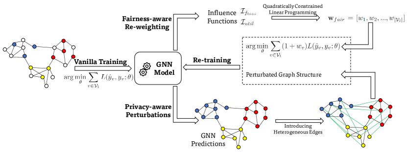
Figure 1: The Framework of Our Privacy-aware Perturbations and Fairness-aware Re-weighting (PPFR) Method. After the vanilla training of a GNN model, the privacy-aware module introduces heterophily edges to generate the perturbed graph structure, fairness-aware re-weighting module employs the influence function and quadratically constrained linear programming to obtain fairness-aware sample weights. After that, the perturbed graph structure and fairness-aware sample weights are involved in the re-training of the target GNN model to promote fairness with limited performance cost and restricted privacy risks.

4.3.1 Fairness-aware Re-weighting.

Inspired by the previous study Li and Liu (2022), we propose to re-weight the training samples to boost fairness with a limited performance cost. Specifically, the weight can be obtained by solving the following Quadratically Constrained Linear Programming (QCLP),

$$\begin{array}[]{ll}\min&\sum\limits_{v\in\mathcal{V}_{l}}w_{v}\mathcal{I}_{f_{bias}}(\mathbf{w}_{v})\\ \mathnormal{s.t.}&\sum\limits_{v\in\mathcal{V}_{l}}w_{v}^{2}\leq\alpha|\mathcal{V}_{l}|,\\ &\sum\limits_{v\in\mathcal{V}_{l}}w_{v}\mathcal{I}_{f_{util}}(\mathbf{w}_{v})\leq\beta\sum\mathcal{I}_{f_{util}}^{+}(\mathbf{w}_{v}),\\ &w_{v}\in[-1,1].\end{array}$$ (13)

In this optimisation, $w_{v}\in[-1,1]$ is the variable. The objective tends to minimise the total bias existing in GNN predictions. The first constraint is designed to control the degree of re-weighting. The second constraint represents that obtained weights only cost limited model utility, where $\mathcal{I}_{f_{util}}^{+}(\mathbf{w}_{v})$ indicates $\mathcal{I}_{f_{util}}(\mathbf{w}_{v})$ with positive value. $\alpha$ and $\beta$ are hyperparameters. In this paper, after solving this QCLP with Gurobi optimiser Gur (2022), the obtained weight of training sample $\mathbf{w}_{fair}=[w_{1},w_{2},...,w_{|\mathcal{V}_{l}|}]$ can be engaged into re-training of the target GNN model with weighted loss in equation (2).

4.3.2 Privacy-aware Perturbations

Given the proposed re-weighting method, a straightforward approach of taking privacy and fairness into account simultaneously is that involving an item that concerns $\mathcal{I}_{f_{risk}}$ into the QCLP (e.g., playing a role as a constraint or part of the objective). However, the negative correlation between $\mathcal{I}_{f_{bias}}$ and $\mathcal{I}_{f_{risk}}$ leads to the weak effectiveness of this simple method. Hence, it is necessary to locate the cause of edge leakage risks and devise a method to restrain it. Next, we will first present the analysis of link-stealing attacks, and then show our perturbation method for inhibiting leakage risks.

(1) Modeling Edge Leakage Risks. In this paper, we take the most practical link-stealing attacks (i.e., Attack-0 in He et al. (2021), black-box setting) as our object. Specifically, in these attacks, after querying the target GNN, attackers can calculate a link score to infer if two nodes are connected based on their prediction similarity. Instead of directly analysing privacy risks in the link score space, we will study it in the embedding space and show how the existence of an edge impacts the learned embedding.

In the embedding space, a well-trained GCN model clusters similar nodes together so that they have similar predictions. According to a previous study Pan et al. (2018), we assume the learned node embedding follows the normal distribution. For simplicity, we employ the left normalisation $\hat{\mathbf{A}}=\tilde{\mathbf{D}}^{-1}(\mathbf{~{}A}+\mathbf{I})$ in GCN models and consider the binary node classification task. Assuming that $\mu_{i}$ and $\sigma$ indicate the mean and standard deviation of the node embedding from class $y_{i}$ ($i=0,1$) at the $t$-th layer, we obtain that the learned embedding $\mathbf{E}^{(t,y_{i})}\sim N(\mu_{i},{\sigma}^{2})$.

In this paper, we focus on analysing the intra-class node pairs (i.e., nodes with the same label), since they are the majority of all node pairs. In a GCN model, edges are involved in the one-hop mean-aggregation operation, i.e., $\hat{\mathbf{A}}\mathbf{E}$. From the view of an individual node $v_{i}$, the one-hop mean-aggregation operation is $[\hat{\mathbf{A}}\mathbf{E}^{(t)}]_{i}=\frac{1}{d_{i}+1}(\mathbf{E}^{(t)}_{i}+\sum_{\begin{subarray}{c}\scriptscriptstyle v_{j}\in\mathcal{N}(v_{i})\\ m_{j}=0\end{subarray}}\mathbf{E}^{(t,y_{0})}_{j}+\sum_{\begin{subarray}{c}\scriptscriptstyle v_{j}\in\mathcal{N}(v_{i})\\ m_{j}=1\end{subarray}}\mathbf{E}^{(t,y_{1})}_{j})$, where $\mathcal{N}(v_{i})$ represents the neighbour node set of $v_{i}$, and ${m}_{i}=1$ indicates $v_{i}$ is from class $y_{1}$, otherwise ${m}_{n}=0$. Given $\mathbf{m}=[m_{1},...,m_{|\mathcal{V}|}]$, $\mathbf{E}^{(t,y_{1})}=diag(\mathbf{m})\mathbf{E}^{(t)}$, $\mathbf{E}^{(t,y_{0})}=(\mathbf{I}-diag(\mathbf{m}))\mathbf{E}^{(t)}$, and $\mathbf{E}^{(t)}=\mathbf{E}^{(t,y_{0})}+\mathbf{E}^{(t,y_{1})}$. Therefore, $\sum_{\begin{subarray}{c}v_{j}\in\mathcal{N}(v_{i})\\ m_{j}=0\end{subarray}}\mathbf{E}_{j}^{(t,y_{0})}\sim N(d_{i}^{y_{0}}\mu_{0},d_{i}^{y_{0}}{\sigma}^{2})$ and $\sum_{\begin{subarray}{c}v_{j}\in\mathcal{N}(v_{i})\\ m_{j}=1\end{subarray}}\mathbf{E}_{j}^{(t,y_{1})}\sim N(d_{i}^{y_{1}}\mu_{1},d_{i}^{y_{1}}{\sigma}^{2})$, where $d_{i}^{y_{0}/y_{1}}$ represent the number of nodes from $\mathbf{E}^{y_{0}/y_{1}}$ and $d_{i}=d_{i}^{y_{0}}+d_{i}^{y_{1}}$ indicate the degree of $v_{i}$. Without loss of generality, we assume that $v_{i}$ and $v_{j}$ in the node pair $(v_{i},v_{j})$ come from class 0.

As shown below, the node distance sensitivity in embedding space can be calculated as the difference between cases where $v_{i}$ and $v_{j}$ are connected or unconnected.

Case 0: When $v_{i}$ and $v_{j}$ is unconnected, $\left(\hat{\mathbf{A}}\mathbf{E}^{(t)}\right)_{i}^{0}$ and $\left(\hat{\mathbf{A}}\mathbf{E}^{(t)}\right)_{j}^{0}$ can be approximately expressed as

$$\left(\hat{\mathbf{A}}\mathbf{E}^{(t)}\right)_{i}^{0}\approx \frac{1}{d_{i}+1}\left(\mathbf{E}^{(t)}_{i}+d_{i}^{y_{0}}\mu_{0}+d_{i}^{y_{1}}\mu_{1}\right),$$ (14)

$$\left(\hat{\mathbf{A}}\mathbf{E}^{(t)}\right)_{j}^{0}\approx \frac{1}{d_{j}+1}\left(\mathbf{E}^{(t)}_{j}+d_{j}^{y_{0}}\mu_{0}+d_{j}^{y_{1}}\mu_{1}\right).$$

Case 1: When $v_{i}$ and $v_{j}$ is connected, $\left(\hat{\mathbf{A}}\mathbf{E}^{(t)}\right)_{i}^{1}$ and $\left(\hat{\mathbf{A}}\mathbf{E}^{(t)}\right)_{j}^{1}$ can be approximately expressed as

$$\left(\hat{\mathbf{A}}\mathbf{E}^{(t)}\right)_{i}^{1}\approx \frac{1}{d_{i}+2}\left(\mathbf{E}^{(t)}_{i}+\mathbf{E}^{(t)}_{j}+d_{i}^{y_{0}}\mu_{0}+d_{i}^{y_{1}}\mu_{1}\right),$$ (15)

$$\left(\hat{\mathbf{A}}\mathbf{E}^{(t)}\right)_{j}^{1}\approx \frac{1}{d_{j}+2}\left(\mathbf{E}^{(t)}_{j}+\mathbf{E}^{(t)}_{i}+d_{j}^{y_{0}}\mu_{0}+d_{j}^{y_{1}}\mu_{1}\right).$$

Given (14) and (15), the distance of $v_{i}$ and $v_{j}$ in the embedding space is calculated as

$$d_{0}(v_{i},v_{j}) =\left(\hat{\mathbf{A}}\mathbf{E}^{(t)}\right)_{i}^{0}-\left(\hat{\mathbf{A}}\mathbf{E}^{(t)}\right)_{j}^{0},$$ (16)

$$d_{1}(v_{i},v_{j}) =\left(\hat{\mathbf{A}}\mathbf{E}^{(t)}\right)_{i}^{1}-\left(\hat{\mathbf{A}}\mathbf{E}^{(t)}\right)_{j}^{1}.$$

Thus, the sensitivity of $d(v_{i},v_{j})$ with respect to the existence of edge $e_{ij}$ is

$$\Delta d(v_{i},v_{j})= \|d_{0}(v_{i},v_{j})-d_{1}(v_{i},v_{j})\|$$ (17)

$$= \left\|\frac{\left(\hat{\mathbf{A}}\mathbf{E}^{(t)}\right)_{i}^{0}-\mathbf{E}^{(t)}_{j}}{d_{i}+2}-\frac{\left(\hat{\mathbf{A}}\mathbf{E}^{(t)}\right)_{j}^{0}-\mathbf{E}^{(t)}_{i}}{d_{j}+2}\right\|,$$

and its expectation is $\mathbb{E}\left[\Delta d(v_{i},v_{j})\right]=\left\|(\mu_{1}-\mu_{0})\delta\right\|$, where $\delta=\frac{d_{i}^{y_{1}}}{(d_{i}+1)(d_{i}+2)}-\frac{d_{j}^{y_{1}}}{(d_{j}+1)(d_{j}+2)}$, due to

$$\mathbb{E}\left[\left(\hat{\mathbf{A}}\mathbf{E}^{(t)}\right)_{i}^{0}-\mathbf{E}^{(t)}_{j}\right] =\frac{(1+d_{i}^{y_{0}})\mu_{0}+d_{i}^{y_{1}}\mu_{1}}{d_{i}+1}-\mu_{0}$$ (18)

$$=\frac{d_{i}^{y_{1}}(\mu_{1}-\mu_{0})}{d_{i}+1},$$

$$\mathbb{E}\left[\left(\hat{\mathbf{A}}\mathbf{E}^{(t)}\right)_{j}^{0}-\mathbf{E}^{(t)}_{i}\right] =\frac{(1+d_{j}^{y_{0}})\mu_{0}+d_{j}^{y_{1}}\mu_{1}}{d_{j}+1}-\mu_{0}$$

$$=\frac{d_{j}^{y_{1}}(\mu_{1}-\mu_{0})}{d_{j}+1}.$$

(2) Perturbation-based Method. Although our modeling process cannot fully depict privacy risks, this coarse grain analysis provides us with insights into understanding risk sources and designing methods to restrict edge leakage. For example, the item $\mu_{0}-\mu_{1}$ in $\mathbb{E}\left[\Delta d(v_{i},v_{j})\right]$ indicates a GNN model with higher performance (i.e., higher discrimination when owning a larger $\mu_{0}-\mu_{1}$ value) has higher edge leakage risks due to the homophily of graph data (i.e., connected nodes are more likely to have similar attributes and the same label). Another item $\delta$ implies that, for nodes with similar degree values, the heterophily difference between nodes is positively correlated to the privacy risk.

According to these insights, we introduce heterophily edge noises into the graph structure to reduce edge leakage risks with a limited performance cost. Specifically, after the vanilla training (i.e., with (1)) of target models, we employ its predictions on all nodes to add heterophily neighbours for each node, i.e.,

$$\mathcal{N}(v_{i})=\mathcal{N}(v_{i})\cup\{v_{i_{1}},...,v_{i_{k}}\},$$ (19)

where the GNN prediction on $v\in\{v_{i_{1}},...,v_{i_{k}}\}$ is different from that on $v_{i}$, $k=\gamma|\mathcal{N}(v_{i})|$ and $\gamma$ is a hype-parameter. With Equation (19) we obtain the perturbed adjacency matrix $\mathbf{A}^{\prime}$, which is involved in the retraining of target GNNs. In addition to reducing heterophily differences between nodes of the same class (i.e., $\delta$ in $\mathbb{E}\left[\Delta d(v_{i},v_{j})\right]$), the introduction of heterophily edges can help close the distance of nodes across classes (i.e., $\mu_{0}-\mu_{1}$ in $\mathbb{E}\left[\Delta d(v_{i},v_{j})\right]$).

4.3.3 Target Model Re-training

Fig. 1 shows the whole framework of our Privacy-aware Perturbations and Fairness-aware Re-weighting (PPFR) method, whose goal is to promote fairness with limited performance costs and restricted privacy risks. The entire training of the target model includes two phases: vanilla training and PPFR retraining. Specifically, we first conduct vanilla training to obtain a competent GNN model. After that, we continue to train (i.e., re-training) the target GNN with the perturbed graph structure and weighted loss function derived from the fairness-aware weights. In PPFR, the epoch number of re-training phase $\mathtt{e}_{re}$ is defined as $\mathtt{e}_{re}=s\mathtt{e}_{va}$, where $\mathtt{e}_{va}$ is the epoch number of vanilla training and $s=0.1$ is a hyper-parameter.

Table 3: Effectiveness of our PPFR method and Correlation between $\mathcal{I}_{f_{bias}}$ and $\mathcal{I}_{f_{risk}}$.

Datasets		$\Delta_{bias}\downarrow$	$\Delta_{risk}\downarrow$	$\Delta\uparrow$	$r$
	Reg	-35.51	1.80	-7.44$\times 10^{-1}$
	DPReg	29.11	-17.07	-1.87$\times 10^{-1}$
	DPFR	-1.17	0.34	-6.55$\times 10^{-3}$
Cora	PPFR	-11.75	-0.73	1.46$\times 10^{-2}$	-0.66
	Reg	-32.36	1.91	-7.17$\times 10^{-1}$
	DPReg	290.34	-14.95	-1.71$\times 10^{0}$
	DPFR	0.22	-0.08	-7.01$\times 10^{-4}$
Citeseer	PPFR	-14.16	-0.31	8.97$\times 10^{-3}$	-0.51
	Reg	-84.70	3.54	-1.28$\times 10^{0}$
	DPReg	-64.45	-32.71	8.81$\times 10^{-1}$
	DPFR	-29.60	0.94	-1.98$\times 10^{-1}$
Pubmed	PPFR	-31.30	-0.18	1.25$\times 10^{-2}$	-0.41

• In this table, columns $\Delta_{bias}$ and $\Delta_{risk}$ show evaluation results in the percentage (i.e.,%) form. In the $\Delta$ column, blue colour represents desired results, while red colour indicates undesired results. “$r$” in the last column indicates the Pearson correlation coefficient between $\mathcal{I}_{f_{bias}}$ and $\mathcal{I}_{f_{risk}}$.

5 Experiments

In this section, we conduct experiments to evaluate our proposed PPFR method. We first introduce the experimental setup, followed by our experimental results and discussion.

5.1 Experimental Setup

Datasets, Models, and Metrics. The datasets, model setup, and fairness and privacy metrics follow that in Section 3.1. Note that the privacy result in this section is the average AUC derived from 8 different distances. Moreover, we use the following metric to evaluate the effect of a method $\Omega$ on both fairness and privacy, i.e.,

$$\Delta =\frac{\Delta_{bias}\Delta_{risk}}{|\Delta_{acc}|},$$ (20)

where $\Delta_{(\cdot)}=\frac{\mathtt{\Omega}_{(\cdot)}-\mathtt{w/o}_{(\cdot)}}{\mathtt{w/o}_{(\cdot)}}$ takes bias/risk/accuracy values of methods $\mathtt{\Omega}$ and $\mathtt{w/o}$ as inputs to evaluate the change ratio on bias/risk/accuracy when using method $\mathtt{\Omega}$, $\mathtt{w/o}$ represents the GNN model obtained by vanilla training. According to the definition, $\Delta$ measures the cost-effectiveness with respect to GNN performance when promoting both fairness and privacy. A positive $\Delta$ indicates that $\mathtt{\Omega}$ can boost fairness and privacy simultaneously, otherwise $\Delta$ is negative.

Baselines. To verify the effectiveness of our method (i.e., PPFR), we combine privacy and fairness methods together as the baseline methods. In this paper, we consider differential privacy (DP) (i.e., EdgeRand and LapGraph Wu et al. (2022b)) as the method to improve edge privacy of GNNs, and both EdgeRand and LapGraph are engaged in generating perturbed adjacency matrix. Specifically, to boost edge privacy, EdgeRand/LapGraph uses a randomisation/Laplacian mechanism to introduce edge noises into the original graph structure. We follow the parameter setting in Wu et al. (2022b) to introduce $\epsilon$-edge DP (i.e., EdgeRand/LapGraph) into our evaluation. According to the previous study Wu et al. (2022b), EdgeRand and LapGraph have similar effectiveness when $\epsilon$ is small, while LapGraph is more applicable to large graphs. Thus, we apply EdgeRand on Cora and Citeseer datasets and LapGraph on the Pubmed dataset.

In this paper, Reg represents that the fairness regularisation is introduced into the loss function of GNN models during their vanilla training. DPReg represents using the edge DP method and adding the fairness regularisation into loss simultaneously. DPFR indicates the combination of edge DP and our fairness-aware re-weighting (FR) in this paper, where a perturbed graph is engaged in the retraining phase.

5.2 Experimental Results

As shown in Table 3, we evaluate the effectiveness of our Privacy-aware Perturbations and Fairness-aware Re-weighting (PPFR) method in boosting fairness with limited performance costs and restricted privacy risks. Results in Table 3 include two parts: correlation results between $\mathcal{I}_{f_{bias}}$ and $\mathcal{I}_{f_{risk}}$, and comparison between our PPFR and baseline methods.

Correlation. In the last column of Table 3, we quantitatively measure the correlation between fairness and privacy with our proposed index (i.e., Eq. 12). The negative correlation results between $\mathcal{I}_{f_{bias}}$ and $\mathcal{I}_{f_{risk}}$ show that there exists a negative correlation between node individual fairness and edge leakage risks. These correlation results are consistent with our observations (i.e., the trade-off between fairness and privacy) in Table 1, and also underpin the design of our PPFR method, that is, it does not involve $\mathcal{I}_{f_{bias}}$ and $\mathcal{I}_{f_{risk}}$ simultaneously in linear programming.

Effectiveness. Other evaluation results also verify the effectiveness of our PPFR method. (1) Due to involving GNN performance into consideration, our PPFR method can maintain the same level of performance as vanilla GNNs on all datasets (i.e., 81.09, 60.50, 81.57 on Cora, Citeseer, and Pubmed, respectively), which is vital in serving GNN users. However, the low performance of DPReg (i.e., 63.26, 47.47, and 64.95 on three datasets, respectively) potentially leads to the impracticability of GNN systems. (2) When comparing the DPFR and PPFR methods, our privacy-aware perturbation (PP) method is more effective than the edge DP methods. Although edge DP (i.e., DPFR rows) is effective in controlling edge leakage risks compared to current fairness promotion methods (e.g., Reg rows), it still poses a higher privacy risk than vanilla GNNs. In contrast, our method is more effective since it presents equal even lower privacy risks in almost all cases, which indicates PPFR can achieve fairness with non-negative privacy impacts. (3) According to the $\Delta$ results, PPFR is the only method that has a positive sign across all datasets, indicating that it can boost fairness and privacy while maintaining competent accuracy.

6 Conclusion

In this paper, we investigate the interaction between the fairness and privacy of GNNs, which is indispensable in comprehensively building trustworthy GNNs. We empirically observe the adverse effects of node fairness on edge privacy risks and propose to quantitatively measure their trade-off through influence functions and Pearson correlation. Finally, we devise a retraining method to increase GNN fairness with limited performance cost and restricted privacy risk, whose effectiveness is demonstrated by our experimental evaluations on real-world datasets. In the future, we will conduct a theoretical analysis between the fairness and privacy of GNNs and explore other methods to balance the different aspects of trustworthy GNNs.

References

- Agarwal et al. [2021] Chirag Agarwal, Himabindu Lakkaraju, and Marinka Zitnik. Towards a unified framework for fair and stable graph representation learning. In UAI, pages 2114–2124. PMLR, 2021.
- Chang and Shokri [2021] Hongyan Chang and Reza Shokri. On the privacy risks of algorithmic fairness. In EuroS&P, pages 292–303. IEEE, 2021.
- Dong et al. [2021] Yushun Dong, Jian Kang, Hanghang Tong, and Jundong Li. Individual fairness for graph neural networks: A ranking based approach. In KDD, pages 300–310. ACM, 2021.
- Gu et al. [2022] Xiuting Gu, Tianqing Zhu, Jie Li, Tao Zhang, Wei Ren, and Kim-Kwang Raymond Choo. Privacy, accuracy, and model fairness trade-offs in federated learning. Comput. Secur., 122:102907, 2022.
- Guo et al. [2022] Xiaojie Guo, Shugen Wang, Hanqing Zhao, Shiliang Diao, Jiajia Chen, Zhuoye Ding, Zhen He, Jianchao Lu, Yun Xiao, Bo Long, et al. Intelligent online selling point extraction for e-commerce recommendation. In Proceedings of the AAAI Conference on Artificial Intelligence, volume 36, pages 12360–12368, 2022.
- Gur [2022] Gurobi optimization, llc. gurobi optimizer reference manual. https://www.gurobi.com/, 2022.
- He et al. [2021] Xinlei He, Jinyuan Jia, Michael Backes, Neil Zhenqiang Gong, and Yang Zhang. Stealing links from graph neural networks. In USENIX Security Symposium, pages 2669–2686. USENIX Association, 2021.
- Kang et al. [2020] Jian Kang, Jingrui He, Ross Maciejewski, and Hanghang Tong. Inform: Individual fairness on graph mining. In KDD, pages 379–389. ACM, 2020.
- Kang et al. [2022] Jian Kang, Qinghai Zhou, and Hanghang Tong. Jurygcn: Quantifying jackknife uncertainty on graph convolutional networks. In KDD, pages 742–752. ACM, 2022.
- Kipf and Welling [2017] Thomas N. Kipf and Max Welling. Semi-supervised classification with graph convolutional networks. In ICLR (Poster). OpenReview.net, 2017.
- Koh and Liang [2017] Pang Wei Koh and Percy Liang. Understanding black-box predictions via influence functions. In ICML, volume 70 of Proceedings of Machine Learning Research, pages 1885–1894. PMLR, 2017.
- Li and Liu [2022] Peizhao Li and Hongfu Liu. Achieving fairness at no utility cost via data reweighing with influence. In ICML, volume 162 of Proceedings of Machine Learning Research, pages 12917–12930. PMLR, 2022.
- Li et al. [2021] Peizhao Li, Yifei Wang, Han Zhao, Pengyu Hong, and Hongfu Liu. On dyadic fairness: Exploring and mitigating bias in graph connections. In ICLR. OpenReview.net, 2021.
- Pan et al. [2018] Shirui Pan, Ruiqi Hu, Guodong Long, Jing Jiang, Lina Yao, and Chengqi Zhang. Adversarially regularized graph autoencoder for graph embedding. In IJCAI, pages 2609–2615. ijcai.org, 2018.
- Sajadmanesh and Gatica-Perez [2021] Sina Sajadmanesh and Daniel Gatica-Perez. Locally private graph neural networks. In CCS, pages 2130–2145. ACM, 2021.
- Sharma et al. [2022] Kartik Sharma, Yeon-Chang Lee, Sivagami Nambi, Aditya Salian, Shlok Shah, Sang-Wook Kim, and Srijan Kumar. A survey of graph neural networks for social recommender systems. CoRR, abs/2212.04481, 2022.
- Wu et al. [2021] Bang Wu, Xiangwen Yang, Shirui Pan, and Xingliang Yuan. Adapting membership inference attacks to GNN for graph classification: Approaches and implications. In ICDM, pages 1421–1426. IEEE, 2021.
- Wu et al. [2022a] Bang Wu, Xiangwen Yang, Shirui Pan, and Xingliang Yuan. Model extraction attacks on graph neural networks: Taxonomy and realization. In AsiaCCS. ACM, 2022.
- Wu et al. [2022b] Fan Wu, Yunhui Long, Ce Zhang, and Bo Li. LINKTELLER: recovering private edges from graph neural networks via influence analysis. In IEEE Symposium on Security and Privacy, pages 2005–2024. IEEE, 2022.
- Wu et al. [2022c] Lingfei Wu, Peng Cui, Jian Pei, and Liang Zhao. Graph Neural Networks: Foundations, Frontiers, and Applications. Springer Singapore, Singapore, 2022.
- Wu et al. [2022d] Yiqing Wu, Ruobing Xie, Yongchun Zhu, Fuzhen Zhuang, Ao Xiang, Xu Zhang, Leyu Lin, and Qing He. Selective fairness in recommendation via prompts. In Proceedings of the 45th International ACM SIGIR Conference on Research and Development in Information Retrieval, pages 2657–2662, 2022.
- Zhang et al. [2020] Yanxin Zhang, Yulei Sui, Shirui Pan, Zheng Zheng, Baodi Ning, Ivor W. Tsang, and Wanlei Zhou. Familial clustering for weakly-labeled android malware using hybrid representation learning. IEEE Trans. Inf. Forensics Secur., 15:3401–3414, 2020.
- Zhang et al. [2021] Tao Zhang, Tianqing Zhu, Kun Gao, Wanlei Zhou, and S Yu Philip. Balancing learning model privacy, fairness, and accuracy with early stopping criteria. IEEE TNNLS, 2021.
- Zhang et al. [2022] He Zhang, Bang Wu, Xingliang Yuan, Shirui Pan, Hanghang Tong, and Jian Pei. Trustworthy graph neural networks: Aspects, methods and trends. CoRR, abs/2205.07424, 2022.
- Zheng et al. [2022] Xin Zheng, Yixin Liu, Shirui Pan, Miao Zhang, Di Jin, and Philip S. Yu. Graph neural networks for graphs with heterophily: A survey. CoRR, abs/2202.07082, 2022.
- Zhu et al. [2019] Rong Zhu, Kun Zhao, Hongxia Yang, Wei Lin, Chang Zhou, Baole Ai, Yong Li, and Jingren Zhou. Aligraph: A comprehensive graph neural network platform. Proc. VLDB Endow., 12(12):2094–2105, 2019.
- Zhu et al. [2021] Jiong Zhu, Ryan A. Rossi, Anup Rao, Tung Mai, Nedim Lipka, Nesreen K. Ahmed, and Danai Koutra. Graph neural networks with heterophily. In AAAI, pages 11168–11176. AAAI Press, 2021.