Hierarchical Programmatic Reinforcement Learning via Learning to Compose Programs

Abstract

Aiming to produce reinforcement learning (RL) policies that are human-interpretable and can generalize better to novel scenarios, Trivedi et al. (2021) present a method (LEAPS) that first learns a program embedding space to continuously parameterize diverse programs from a pre-generated program dataset, and then searches for a task-solving program in the learned program embedding space when given a task. Despite the encouraging results, the program policies that LEAPS can produce are limited by the distribution of the program dataset. Furthermore, during searching, LEAPS evaluates each candidate program solely based on its return, failing to precisely reward correct parts of programs and penalize incorrect parts. To address these issues, we propose to learn a meta-policy that composes a series of programs sampled from the learned program embedding space. By learning to compose programs, our proposed hierarchical programmatic reinforcement learning (HPRL) framework can produce program policies that describe out-of-distributionally complex behaviors and directly assign credits to programs that induce desired behaviors. The experimental results in the Karel domain show that our proposed framework outperforms baselines. The ablation studies confirm the limitations of LEAPS and justify our design choices.

formats numbers=left, stepnumber=1, numberstyle=, numbersep=10pt, numberstyle=

1 Introduction

Deep reinforcement learning (DRL) leverages the recent advancement in deep learning by reformulating the reinforcement learning problem as learning policies or value functions parameterized by deep neural networks. DRL has achieved tremendous success in various domains, including controlling robots (Gu et al., 2017; Ibarz et al., 2021; Lee et al., 2019, 2021), playing board games (Silver et al., 2016, 2017), and strategy games (Vinyals et al., 2019; Wurman et al., 2022). Yet, the black-box nature of neural network-based policies makes it difficult for the DRL-based systems to be interpreted and therefore trusted by human users (Lipton, 2016; Puiutta & Veith, 2020). Moreover, policies learned by DRL methods tend to overfit and often fail to generalize (Zhang et al., 2018; Cobbe et al., 2019; Sun et al., 2020a; Liu et al., 2022).

To address the abovementioned issues of DRL, programmatic RL methods (Bastani et al., 2018; Inala et al., 2020; Landajuela et al., 2021; Verma et al., 2018) explore various of more structured representations of policies, such as decision trees and state machines. In particular, Trivedi et al. (2021) present a framework, Learning Embeddings for lAtent Program Synthesis (LEAPS), that is designed to produce more interpretable and generalizable policies. Specifically, it aims to produce program policies structured in a given domain-specific language (DSL), which can be executed to yield desired behaviors. To this end, LEAPS first learns a program embedding space to continuously parameterize diverse programs from a pre-generated program dataset, and then searches for a task-solving program in the learned program embedding space when given a task described by a Markov Decision Process (MDP). The program policies produced by LEAPS are not only human-readable but also achieve competitive performance and demonstrate superior generalization ability.

Despite its encouraging results, LEAPS has two fundamental limitations. Limited program distribution: the program policies that LEAPS can produce are limited by the distribution of the pre-generated program dataset used for learning the program embedding space. This is because LEAPS is designed to search for a task-solving program from the learned embedding space, which inherently assumes that such a program is within the distribution of the program dataset. Such design makes it difficult for LEAPS to synthesize programs that are out-of-distributionally long or complex. Poor credit assignment: during the search for the task-solving program embedding, LEAPS evaluates each candidate program solely based on the cumulative discounted return of the program execution trace. Such design fails to accurately attribute rewards obtained during the execution trajectories to corresponding parts in synthesized programs or penalize program parts that induce incorrect behaviors.

This work aims to address the issues of limited program distribution and poor credit assignment. To this end, we propose a hierarchical programmatic reinforcement learning (HPRL) framework. Instead of searching for a program from a program embedding space, we propose to learn a meta-policy, whose action space is the learned program embedding space, to produce a series of programs (i.e., predict a sequence of actions) to yield a composed task-solving program. By re-formulating synthesizing a program as predicting a sequence of programs, HPRL can produce out-of-distributionally long or complex programs. Also, rewards obtained from the environment by executing each program from the composed program can be accurately attributed to each program, leading to more efficient learning.

To evaluate our proposed method, we adopt the Karel domain (Pattis, 1981), which features an agent that can navigate a grid world and interact with objects. Our method outperforms all the baselines by large margins on a problem set proposed in (Trivedi et al., 2021). To investigate the limitation of our method, we design a more challenging problem set on which our method consistently achieves better performance compared to LEAPS. Moreover, we inspect LEAPS’ issues of limited program distribution and poor credit assignment with two experiments and demonstrate that our proposed method addresses these issues. We present a series of ablation studies to justify our design choices, including the reinforcement learning algorithms used to learn the meta-policy, and the dimensionality of the program embedding space.

2 Related Work

Program Synthesis. Program synthesis methods concern automatically synthesize programs that can transform some inputs to desired outputs. Encouraging results have been achieved in a variety of domains, including string transformation (Devlin et al., 2017; Hong et al., 2021; Zhong et al., 2023), array/tensor transformation (Balog et al., 2017; Ellis et al., 2020), computer commands (Lin et al., 2018; Chen et al., 2021; Li et al., 2022), graphics and 3D shape programs (Wu et al., 2017; Liu et al., 2019; Tian et al., 2019), and describing behaviors of agents (Bunel et al., 2018; Sun et al., 2018; Shin et al., 2018; Chen et al., 2019; Liao et al., 2019; Silver et al., 2020). Most existing program synthesis methods consider task specifications such as input/output pairs, demonstrations, or natural language descriptions. In contrast, we aim to synthesize programs as policies that can be executed to induce behaviors which maximize rewards defined by reinforcement learning tasks.

Programmatic Reinforcement Learning. Programmatic reinforcement learning methods (Choi & Langley, 2005; Winner & Veloso, 2003; Sun et al., 2020a) explore various programmatic and more structured representations of policies, including decision trees (Bastani et al., 2018), state machines (Inala et al., 2020), symbolic expressions (Landajuela et al., 2021), and programs drawn from a domain-specific language (Silver et al., 2020; Verma et al., 2018, 2019). Our work builds upon (Trivedi et al., 2021), whose goal is to produce program policies from rewards. We aim to address the fundamental limitations of this work by learning to compose programs to yield more expressive programs.

Hierarchical Reinforcement Learning (HRL). HRL frameworks  (Sutton et al., 1999; Barto & Mahadevan, 2003; Vezhnevets et al., 2017; Bacon et al., 2017) aims to learn to operate on different levels of temporal abstraction, allowing for learning or exploring more efficiently in sparse-reward environments. In this work, instead of operating on pre-defined or learned temporal abstraction, we are interested in learning with a level of abstraction defined by a learned program embedding space to hierarchically compose programs. One can view a learned program embedding space as continuously parameterized options or low-level policies.

Program Induction. Program induction (Graves et al., 2014; Zaremba & Sutskever, 2015; Reed & De Freitas, 2016; Dong et al., 2019; Ellis et al., 2021) aims to perform tasks by inducing latent programs for improved generalization. Contrary to our work, these methods neither explicitly synthesize programs nor address RL tasks.

3 Problem Formulation

$\displaystyle\text{Program}\ \rho$ $\displaystyle\coloneqq\text{DEF}\ \text{run}\ \text{m}(\ s\ \text{m})$ $\displaystyle\text{Repetition}\ n$ $\displaystyle\coloneqq\text{Number of repetitions}$ $\displaystyle\text{Perception}\ h$ $\displaystyle\coloneqq\text{frontIsClear}\ |\ \text{leftIsClear}\ |\ \text{rightIsClear}\ |\$ $\displaystyle\text{markerPresent}\ |\ \text{noMarkerPresent}$ $\displaystyle\text{Condition}\ b$ $\displaystyle\coloneqq\text{perception h}\ |\ \text{not}\ \text{perception h}$ $\displaystyle\text{Action}\ a$ $\displaystyle\coloneqq\text{move}\ |\ \text{turnLeft}\ |\ \text{turnRight}\ |\$ $\displaystyle\text{putMarker}\ |\ \text{pickMarker}$ $\displaystyle\text{Statement}\ s$ $\displaystyle\coloneqq\text{while}\ \text{c}(\ b\ \text{c})\ \text{w}(\ s\ \text{w})\ |\ s_{1};s_{2}\ |\ a\ |$ $\displaystyle\ \text{repeat}\ \text{R=}n\ \text{r}(\ s\ \text{r})\ |\ \text{if}\ \text{c}(\ b\ \text{c})\ \text{i}(\ s\ \text{i})\ |$ $\displaystyle\ \text{ifelse}\ \text{c}(\ b\ \text{c})\ \text{i}(\ s_{1}\ \text{i})\ \text{else}\ \text{e}(\ s_{2}\ \text{e})$

Figure 1: The domain-specific language (DSL) for the Karel domain, features an agent that can navigate through a grid world and interact with objects.

Our goal is to develop a method that can synthesize a domain-specific, task-solving program which can be executed to interact with an environment and maximize a discounted return defined by a Markov Decision Process.

Domain Specific Language. In this work, we adapt the domain-specific language (DSL) for the Karel domain used in (Bunel et al., 2018; Chen et al., 2019; Trivedi et al., 2021), shown in Figure 1. This DSL is designed to describe the behaviors of the Karel agent, consisting of control flows, agent’s perceptions, and agent’s actions. Control flows such as if, else, and while are allowed for describing diverging or repetitive behaviors. Furthermore, Boolean and logical operators such as and, or, and not can be included to express more sophisticated conditions. Perceptions such as frontIsClear and markerPresent are defined based on situations in an environment which can be perceived by an agent. On the other hand, actions such as move, turnRight, and putMarker, describe the primitive behaviors that an agent can perform in an environment. A program policy considered in our work is structured in this DSL and can be executed to produce a sequence of actions based on perceptions.

Markov Decision Process (MDP). The tasks considered in this work are defined by finite-horizon discounted MDPs. The performance of a policy with its rollout (a sequence of states and actions $\{(s_{0},a_{0}),...,(s_{t},a_{t})\}$) is evaluated based on a discounted return $\sum_{t=0}^{T}\gamma^{t}r_{t}$, where $r_{t}=\mathcal{R}(s_{t},a_{t})$ indicates the reward function and $T$ is the horizon of the episode. We aim to develop a method that can produce a program representing a policy that can be executed to maximize the discounted return, i.e., $\max_{\rho}\mathbb{E}_{a\sim\text{EXEC}(\rho)}[\sum_{t=0}^{T}\gamma^{t}r_{t}]$, where EXEC$(\cdot)$ returns the actions induced by executing the program policy $\rho$ in the environment. This objective is a special case of the standard RL objective where a policy is represented as a program in a DSL and the policy rollout is obtained by executing the program.

4 Approach

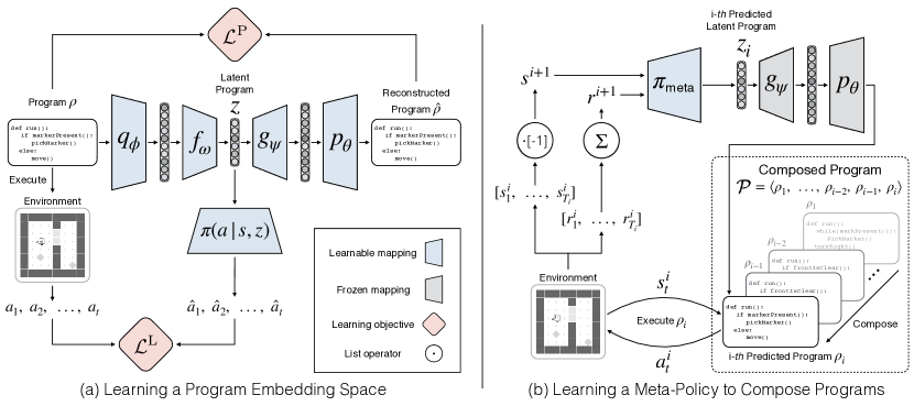
Figure 2: Hierarchical Programmatic Reinforcement Learning. (a) Learning a Program Embedding Space: a continuously parameterized latent program space can be learned using the program encoder $q_{\phi}$, decoder $p_{\theta}$, and a neural executor policy $\pi$ by optimizing the two reconstruction objectives: $\mathcal{L}^{P}$ and $\mathcal{L}^{L}$. To reduce the dimensionality of the program embedding space to facilitate task learning, we employ a compression encoder $f_{\omega}$ and a compression decoder $g_{\psi}$. (b) Learning a Meta-Policy to Compose Programs: given a task described by an MDP, we propose to train a meta-policy $\pi_{meta}$ to compose a sequence of programs, and yield a task-solving program. Specifically, at each macro time step $i$, the meta-policy $\pi_{meta}$ predicts a latent program embedding $z_{i}$, which can be decoded to the corresponding program $\rho_{i}=p_{\theta}(g_{\psi}(z_{i}))$. We then execute the program $\rho_{i}$ in the environment, which returns the cumulative reward $r^{i+1}$ and the next state $s^{i+1}$ to the meta policy. Then, the meta-policy can synthesize the next program $\rho_{i+1}$ based on $s^{i+1}$. Upon termination, the predicted task-solving program is composed of a series of synthesized programs $\mathcal{P}=\langle\rho_{1},\rho_{2},...,\rho_{|H|-1},\rho_{|H|}\rangle$.

Our goal is to design a framework that can synthesize task-solving programs based on the rewards obtained from MDPs. We adapt the idea of learning a program embedding space to continuously parameterized a diverse set of programs proposed in LEAPS (Trivedi et al., 2021). Then, instead of searching for a task-solving program in the learned program embedding space, our key insight is to learn a meta-policy that can hierarchically compose programs to form a more expressive task-solving program. Our proposed framework, dubbed Hierarchical Programmatic Reinforcement Learning (HPRL), is capable of producing out-of-distributionally long and complex programs. Moreover, HPRL can make delicate adjustments to synthesized programs according to rewards obtained from the environment.

Section 4.1 presents how LEAPS learns a program embedding space to continuously parameterize a set of randomly generated programs and describes our proposed procedure to produce a dataset containing more diverse programs. Then, to reduce the dimension of the learned program embedding for more efficient meta-policy learning, Section 4.2 introduces how we compress the embedding space. Finally, in Section 4.3, we describe our method for learning a meta-policy, whose action space is the learned program embedding space, to hierarchically compose programs and yield a task-solving program. An overview of our proposed framework is illustrated in Figure 2.

4.1 Learning a Program Embedding Space

We aim to learn a program embedding space that continuously parameterizes a diverse set of programs. Moreover, a desired program embedding space should be behaviorally smooth, i.e., programs that induce similar execution traces should be embedded closely to each other and programs with diverging behaviors should be far from each other in the embedding space.

To this end, we adapt the technique proposed in LEAPS (Trivedi et al., 2021), which trains an encoder-decoder neural network architecture on a pre-generated program dataset. Specifically, a recurrent neural network program encoder $q_{\phi}$ learns to encode a program $\rho$ (i.e., sequences of program tokens) into a program embedding space, yielding a program embedding $v$; a recurrent neural network program decoder $p_{\theta}$ learns to decode a program embedding $v$ to produce reconstructed programs $\hat{\rho}$. The program encoder and the program decoder are trained to optimize the $\beta$-VAE (Higgins et al., 2016) objective:

$$\begin{split}\mathcal{L}_{\theta,\phi}^{\text{P}}(\rho)=-\mathbb{E}_{v\sim q_{\phi}(v|\rho)}[\log p_{\theta}(\rho|v)]\\ +\beta D_{\text{KL}}(q_{\phi}(v|\rho)\|p_{\theta}(v)),\end{split}$$ (1)

where $\beta$ balances the reconstruction loss and the representation capacity of the program embedding space (i.e., the latent bottleneck).

To encourage behavioral smoothness, Trivedi et al. (2021) propose two additional objectives. The program behavior reconstruction loss minimizes the difference between the execution traces of the given program EXEC($\rho$) and the execution traces of the reconstructed program EXEC($\hat{\rho}$). On the other hand, the latent behavior reconstruction loss brings closer the execution traces of the given program EXEC($\rho$) and the execution traces produced by feeding the program embedding $v$ to a learned neural program executor $\pi(a|v,s)$:

$$\begin{split}\mathcal{L}_{\pi,\phi}^{\text{L}}(\rho,\pi)=-\mathbb{E}_{v\sim q_{\phi}(v|\rho)}[\sum_{t=1}^{H}\sum_{i=1}^{|\mathcal{A}|}\text{EXEC}_{t,i}(\rho)\\ \log\pi(a_{i}|v,s_{t})],\end{split}$$ (2)

where $H$ denotes the horizon of EXEC($\rho$), $|\mathcal{A}|$ denotes the cardinality of the action space, and $\text{EXEC}_{t,i}(\rho)$ is the boolean function indicating if the action equals to $a_{i}$ at time step $t$ while executing program $\rho$.

We empirically found that optimizing the program behavior reconstruction loss does not yield a significant performance gain. Yet, due to the non-differentiability nature of program execution, optimizing this loss via REINFORCE (Williams, 1992) is unstable. Moreover, performing on-the-fly program execution during training significantly slows down the learning process. Therefore, we exclude the program behavior reconstruction loss, yielding our final objective for learning a program embedding space as a combination of the $\beta$-VAE objective $\mathcal{L}_{\theta,\phi}^{\text{P}}$ and the latent behavior reconstruction loss $\mathcal{L}_{\pi}^{\text{L}}$:

$$\min_{\theta,\phi,\pi}\mathcal{L}_{\theta,\phi}^{\text{P}}(\rho)+\lambda\mathcal{L}_{\pi}^{\text{L}}(\rho,\pi),$$ (3)

where $\lambda$ determines the relative importance of these losses.

4.2 Compressing the Learned Program Embedding Space

The previous section describes a method for constructing a program embedding space that continuously parameterizes programs. Next, given a task defined by an MDP, we aim to learn a meta-policy that predicts a sequence of program embeddings as actions to compose a task-solving program. Hence, a low-dimensional program embedding space (i.e., a smaller action space) is ideal for efficiently learning such a meta-policy. Yet, to embed a large number of programs with diverse behaviors, a learned program embedding space needs to be extremely high-dimensional.

Therefore, our goal is to bridge the gap between a high-dimensional program embedding space with sufficient representation capacity and a desired low-dimensional action space for learning a meta-policy. To this end, we augment the encoder-decoder architecture with additional fully-connected layers to further reduce the program embedding space. Specifically, we employ a compression encoder $f_{\omega}$ that takes the output of the program encoder $q_{\phi}$ as input and compresses it into a lower-dimensional program embedding $z$; also, we employ a compression decoder $g_{\psi}$ that takes a program embedding as input and decompresses it to produce a reconstructed higher-dimensional program embedding $\hat{v}$, which is then fed to the program decoder $p_{\theta}$ to produce a reconstructed program $\hat{\rho}$.

With this modification, the $\beta$-VAE objective and the latent behavior reconstruction loss can be rewritten as:

$$\begin{split}\mathcal{L}_{\theta,\phi,\omega,\psi}^{\text{P}}(\rho)=-\mathbb{E}_{z\sim f_{\omega}(z|q_{\phi}(\rho))}[\log p_{\theta}(\rho|(g_{\psi}(z)))]\\ +\beta D_{\text{KL}}(f_{\omega}(q_{\phi}(z|\rho))\|p_{\theta}(g_{\psi}(z))),\end{split}$$ (4)

and

$$\begin{split}\mathcal{L}_{\pi,\omega,\phi}^{\text{L}}(\rho,\pi)=-\mathbb{E}_{z\sim f_{\omega}(z|q_{\phi}(\rho))}[\sum_{t=1}^{H}\sum_{i=1}^{|\mathcal{A}|}\text{EXEC}_{t,i}(\rho)\\ \log\pi(a_{i}|z,s_{t})],\end{split}$$ (5)

We train the program encoder $q_{\phi}$, the compression encoder $f_{\omega}$, the compression decoder $g_{\psi}$, the program decoder $p_{\theta}$, and the neural execution policy $\pi$ in an end-to-end manner as described in Algorithm 1. We discuss how the dimension of the program embedding space affects the quality of latent program embedding space in Section 5.4.2.

Algorithm 1 HPRL: Learning Latent Program Embedding Space

Input: Program Dataset $D_{program}$, Training Epoch $N_{epoch}$
Output: Compression Decoder $g_{\psi}$, Program Decoder $p_{\theta}$

1:  Initialize the program encoder $q_{\phi}$ and decoder $p_{\theta}$, compression encoder $f_{\omega}$ and decoder $g_{\psi}$, neural execution policy $\pi$.

2:  for epoch in range(1, $N_{epoch}$) do

3:     for program $\rho$ in $D_{program}$ do

4:        $z=f_{\omega}(q_{\phi}(\rho))$

5:        $\hat{\rho}=p_{\theta}(g_{\psi}(z))$

6:        Compute $\mathcal{L}_{total}=\mathcal{L}^{P}_{\theta,\phi,\omega,\phi}(\rho)+\lambda\mathcal{L}^{L}_{\pi,\omega,\phi}(\rho,\pi)$

7:        Fit $\phi,\omega,\psi,\theta,\pi$ to minimize $\mathcal{L}_{total}$

8:     end for

9:  end for

4.3 Learning a Meta-Policy to Compose the Task-Solving Program

Once an expressive, smooth, yet compact program embedding space is learned, given a task described by an MDP, we propose to train a meta-policy $\pi_{\text{meta}}$ following Algorithm 2 to compose a task-solving program. Specifically, the learned program embedding space is used as a continuous action space for the meta-policy $\pi_{\text{meta}}$. We formulate the task of composing programs as a finite-horizon MDP whose horizon is $|H|$. At each time step $i$, the meta-policy $\pi_{\text{meta}}$ takes an input state $s^{i}$ and predicts one latent program embedding $z_{i}$ as action, which can be decoded to its corresponding program $\rho_{i}$ using the learned compression decoder and program decoder $p_{\theta}(g_{\psi}(z_{i}))$. Then, the program $\rho_{i}$ is executed with $\text{EXEC}(\cdot)$ to interact with the environment for a period from $1$ to $T^{i}$, yielding the cumulative reward $r^{i+1}=\sum_{t=1}^{T^{i}}r^{i}_{t}$ and the next state $s^{i+1}=[s^{i}_{1},s^{i}_{2},...,s^{i}_{T_{i}}][-1]$ after the program execution. The operator $\cdot[-1]$ returns the last object in the sequence, and we take the last state of the program execution as the next macro input state, i.e., $s^{i+1}=[s^{i}_{1},s^{i}_{2},...,s^{i}_{T_{i}}][-1]=s^{i}_{T_{i}}$. A program will terminate when it is fully executed or once 100 actions have been triggered. Note that the time steps $i$ considered here are macro time steps, each involves a series of state transitions and returns a sequence of rewards. The environment will return the next state $s^{i+1}$ and cumulative reward $r^{i+1}$ to the agent to predict the next latent program embedding $z_{i+1}$. The program composing process terminates after repeating $|H|$ steps.

The synthesized task-solving program $\mathcal{P}$ is obtained by sequentially composing the generated program $\langle\rho_{i}|i=1...|H|\rangle$, where $\langle\cdot\rangle$ denotes an operator that concatenates programs in order to yield a composed program. Hence, the learning objective of the meta-policy $\pi_{\text{meta}}$ is to maximize the total cumulative return $\mathcal{J}_{\pi_{\text{meta}}}$:

$$\mathcal{J}_{\pi_{\text{meta}}}=\mathbb{E}_{\mathcal{P}\sim\pi_{\textsc{meta}}}[\sum_{i=1}^{|H|}\gamma^{i-1}\mathbb{E}_{a\sim\text{EXEC}(\rho_{i})}[r^{i+1}].$$ (6)

where $\gamma$ is the discount factor for macro time steps MDP and $a$ is the primitive action triggered by $\text{EXEC}(\rho_{i})$. We detail the meta-policy training procedure in Algorithm 2.

Algorithm 2 HPRL: Meta-Policy Training

Input: Program Decoder $p_{\theta}$, Compression Decoder $g_{\psi}$, Meta-Policy Training Step $T_{meta}$, Horizon $|H|$
Output: Task Solving Program $\mathcal{P}$

1:  Initialize a meta-policy $\pi_{meta}$

2:  Load and fix $p_{\theta},g_{\psi}$ for Meta-Policy Training

3:  for Training Episode in range(1, $T_{meta}/|H|$) do

4:     Receive initial state $s^{1}$ from the Karel environment

5:     for i in range(1, $|H|$) do

6:        $z_{i}=\pi_{meta}(s^{i})$

7:        $\rho_{i}=p_{\theta}(g_{\psi}(z_{i}))$

8:        Interact with the environment by EXEC($\rho_{i}$)

9:        Receive $[s^{i}_{1},...,s^{i}_{T}]$ and $[r^{i}_{1},...,r^{i}_{T_{i}}]$

10:        $r^{i+1}=\sum_{t=1}^{T^{i}}r^{i}_{t}$

11:        $s^{i+1}=[s^{i}_{1},s^{i}_{2},...,s^{i}_{T_{i}}][-1]$

12:     end for

13:     Calculate $\mathcal{J}_{\pi_{meta}}$ based on the collected $\{(s^{i},z^{i},r^{i+1},s^{i+1})|i=1,...,|H|\}$

14:     Optimize $\pi_{meta}$ to maximize $\mathcal{J}_{\pi_{meta}}$

15:  end for

While this work formulates the program synthesis task as a finite-horizon MDP where a fixed number of programs $|H|$ are composed, we can instead learn a termination function that decides when to finish the program composition process, which is left to future work.

5 Experiments

We design and conduct experiments to compare our proposed framework (HPRL) to its variants and baselines.

5.1 Karel domain

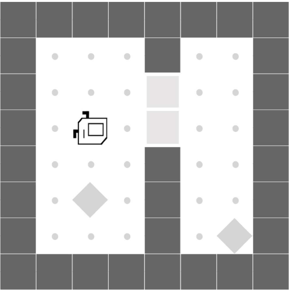
(a) DoorKey

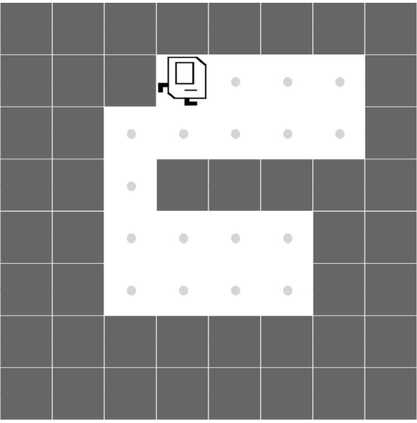
(b) OneStroke

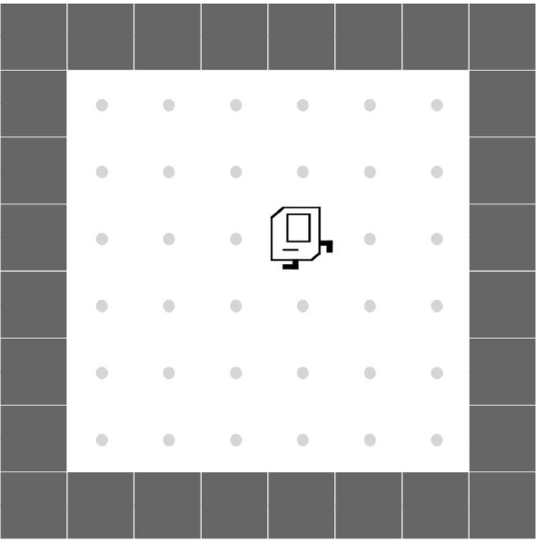
(c) Seeder

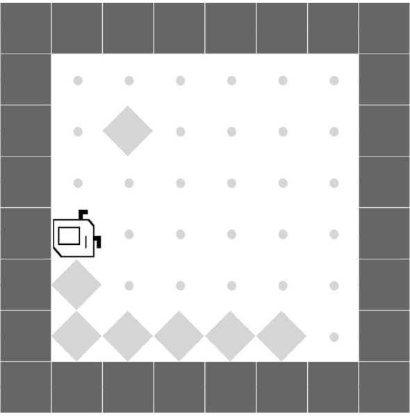
(d) Snake

Figure 3: Karel-Hard Problem Set: The four tasks require an agent to acquire a set of diverse, goal-oriented, and programmatic behaviors. This is strictly more challenging compared to the Karel problem set proposed in (Trivedi et al., 2021).

For the experiments and ablation studies, we adopt the Karel domain (Pattis, 1981), which is widely used in program synthesis and programmatic reinforcement learning (Bunel et al., 2018; Shin et al., 2018; Sun et al., 2018; Chen et al., 2019; Trivedi et al., 2021). The Karel agent in a gridworld can navigate and interact with objects (i.e., markers). The action and perception are detailed in Figure 1.

To evaluate the proposed framework and the baselines, we consider two problem sets. First, we use the Karel problem set proposed in (Trivedi et al., 2021), which consists of six tasks. Then, we propose a more challenging set of tasks, Karel-Hard problem set (shown in Figure 3), which consists of four tasks. In most tasks, initial configurations such as agent and goal locations, wall and marker placement, are randomly sampled upon every episode reset.

Karel Problem Set. The Karel problem set introduced in (Trivedi et al., 2021) consists of six tasks: StairClimber, FourCorner, TopOff, Maze, CleanHouse and Harvester. Solving these tasks requires the following ability. Repetitive Behaviors: to conduct the same behavior for several times, i.e., placing markers on all corners (FourCorner) or move along the wall (StairClimber). Exploration: to navigate the agent through complex patterns (Maze) or multiple chambers (CleanHouse). Complexity: to perform specific actions, i.e., put markers on marked grid (TopOff) or pick markers on marked grid (Harvester). For further description about the Karel problem set, please refer to Section C.1.

Karel-Hard Problem Set. We design a more challenging set of tasks, the Karel-Hard problem set. The ability required to solve the tasks in this problem set can be categorized as follows: Two-stage exploration: to explore the environment under different conditions, i.e., pick up the marker in one chamber to unlock the door, and put the marker in the next chamber (DoorKey). Additional Constraints: to perform specific actions under restrictions, i.e., traverse the environment without revisiting the same position (OneStroke), place exactly one marker on all grids (Seeder), and traverse the environment without hitting a growing obstacle (Snake). More details about the Karel-Hard problem set can be found in Section C.2.

5.2 Experimental Settings

Section 5.2.1 introduces the procedure for generating the program dataset used for learning a program embedding space. The implementation of the proposed framework is described in Section 5.2.2.

5.2.1   Karel DSL Program Dataset Generation with Our Improved Generation Procedure

The Karel program dataset used in this work includes one million programs. All the programs are generated based on syntax rules of the Karel DSL with a maximum length of $40$ program tokens. While Trivedi et al. (2021) randomly sample to generate program sequences, we propose an improved program generation procedure as follows. We filter out counteracting programs (e.g., termination state equals initial state after program execution), repetitive programs (e.g., programs with long common sub-sequences) and programs with canceling action sequences (e.g., turnLeft followed by turnRight). These rules significantly improve the diversity and expressiveness of the generated programs and induce a more diverse and complex latent program space. More details can be found in Section E.

5.2.2   Implementation

Encoders & Decoders. We use GRU (Cho et al., 2014) layer to implement both the program encoder $q_{\phi}$ and the program decoder $p_{\theta}$ mentioned in Section 4.1 with a hidden dimension of $256$. The last hidden state of the encoder $q_{\phi}$ is taken as the uncompressed program embedding $v$. This program embedding $v$ can be further compressed to a $64$-dimensional program embedding $z$ using the compression encoder $f_{\omega}$ and compression decoder $g_{\psi}$ constructed by the fully-connected neural network as described in Section 4.2.

Neural Program Executor. The neural program executor $\pi$ is implemented as a recurrent conditional policy $\pi(\cdot|z,s)$ using GRU layers, which takes the abstract state $s$ and the program embedding $z$ at each time step as input and predicts the execution trace.

Meta-Policy. To implement the meta-policy $\pi_{\text{meta}}$, we use convolutional layers (Fukushima & Miyake, 1982; Krizhevsky et al., 2017) to extract features from the Karel states and then process them with GRU layers for predicting program embeddings. To optimize the meta-policy, we use two popular reinforcement learning algorithms, PPO (Schulman et al., 2017) and SAC (Haarnoja et al., 2018), and report their experimental results as HPRL-PPO and HPRL-SAC, respectively.

More details on hyperparameters, training procedure, and implementation can be found in Section D.

Table 1: Mean return and standard deviation of all methods across the Karel problem set, evaluated over five random seeds. HPRL-PPO outperforms all prior approaches and achieves the maximum score on all tasks. HPRL-SAC completely solves four out of six tasks.

Method	StairClimber	FourCorner	TopOff	Maze	CleanHouse	Harvester
Best-Sampled	1.00 $\pm$ 0.00	0.25 $\pm$ 0.00	0.60 $\pm$ 0.07	1.00 $\pm$ 0.00	0.05 $\pm$ 0.04	0.17 $\pm$ 0.00
DRL	1.00 $\pm$ 0.00	0.29 $\pm$ 0.05	0.32 $\pm$ 0.07	1.00 $\pm$ 0.00	0.00 $\pm$ 0.00	0.90 $\pm$ 0.10
DRL-abs	0.13 $\pm$ 0.29	0.36 $\pm$ 0.44	0.63 $\pm$ 0.23	1.00 $\pm$ 0.00	0.01 $\pm$ 0.02	0.32 $\pm$ 0.18
VIPER	0.02 $\pm$ 0.02	0.40 $\pm$ 0.42	0.30 $\pm$ 0.06	0.69 $\pm$ 0.05	0.00 $\pm$ 0.00	0.51 $\pm$ 0.07
LEAPS	1.00 $\pm$ 0.00	0.45 $\pm$ 0.40	0.81 $\pm$ 0.07	1.00 $\pm$ 0.00	0.18 $\pm$ 0.14	0.45 $\pm$ 0.28
LEAPS-ours	1.00 $\pm$ 0.00	0.50 $\pm$ 0.47	0.82 $\pm$ 0.11	1.00 $\pm$ 0.00	0.28 $\pm$ 0.27	0.82 $\pm$ 0.16
HPRL-SAC	1.00 $\pm$ 0.00	1.00 $\pm$ 0.00	0.61 $\pm$ 0.25	1.00 $\pm$ 0.00	0.99 $\pm$ 0.02	1.00 $\pm$ 0.00
HPRL-PPO	1.00 $\pm$ 0.00	1.00 $\pm$ 0.00	1.00 $\pm$ 0.00	1.00 $\pm$ 0.00	1.00 $\pm$ 0.00	1.00 $\pm$ 0.00

Table 2: Mean return and standard deviation of all methods across the Karel-Hard problem set, evaluated over five random seeds. HPRL-PPO achieves best performance across all tasks.

Method	DoorKey	OneStroke	Seeder	Snake
Best-Sampled	0.50 $\pm$ 0.00	0.55 $\pm$ 0.34	0.17 $\pm$ 0.00	0.20 $\pm$ 0.00
LEAPS	0.50 $\pm$ 0.00	0.65 $\pm$ 0.19	0.51 $\pm$ 0.21	0.21 $\pm$ 0.15
LEAPS-ours	0.50 $\pm$ 0.00	0.72 $\pm$ 0.06	0.57 $\pm$ 0.02	0.25 $\pm$ 0.07
HPRL-SAC	0.50 $\pm$ 0.00	0.76 $\pm$ 0.05	0.27 $\pm$ 0.10	0.28 $\pm$ 0.15
HPRL-PPO	0.50 $\pm$ 0.00	0.80 $\pm$ 0.02	0.58 $\pm$ 0.07	0.28 $\pm$ 0.11

5.2.3   Baseline Approaches

We compare HPRL with the following baselines.

• Best-sampled. It randomly samples $1000$ programs from the learned program embedding space and reports the highest return achieved by the sampled programs.

• DRL and DRL-abs. Deep RL baselines from (Trivedi et al., 2021). DRL observes a raw state (grids) input from the Karel environment, while DRL-abs is a recurrent neural network policy that takes abstracted state vectors from the environment as input. The abstracted state vectors consist of binary values of the current state (e.g., [frontIsClear() == True, markerPresent()==False, ...]).

• VIPER. A programmatic RL method proposed by Bastani et al. (2018). It uses a decision tree to imitate the behavior of a learned DRL policy.

• LEAPS. A programmatic RL framework proposed by Trivedi et al. (2021) that uses Cross-Entropy Method (Rubinstein, 1997) to search task-solving program in a learned continuous program embedding space.

• LEAPS-ours. The LEAPS framework trained on the proposed Karel program dataset described in Section 5.2.1. This is used to compare our proposed program dataset generation procedure with the generation approach used in (Trivedi et al., 2021).

More details of these baselines can be found in  Section B.

5.3 Experimental Results

We evaluate the cumulative return of all methods on the Karel problem set and the Karel-Hard problem set. The results of the two problem sets are presented in Table 1 and Table 2, respectively. The range of the cumulative return is within $[0,1]$ on all tasks. Section C describes the detailed definition of the reward function for each task. The performance of DRL, DRL-abs, VIPER, and LEAPS reproduced with the implementation provided by Trivedi et al. (2021). The average cumulative return and standard deviation of all the methods on each task are evaluated over five random seeds to ensure statistical significance.

Overall Karel Performance. The experimental results on Table 1 show that HPRL-PPO outperforms all other approaches on all tasks. Furthermore, HPRL-PPO can completely solve all the tasks in the Karel problem set. The Best-sampled results justify the quality of the learned latent space as tasks like StairClimber and maze can be entirely solved by one (or some) of 1000 randomly sampled programs. However, all 1000 randomly sampled programs fail on tasks that require long-term planning and exploration (e.g., FourCorner, CleanHouse and Harvester), showing the limit of the simple search-based method. On the other hand, we observe that LEAPS-ours outperforms LEAPS on all of the six tasks in the Karel problem set, showing that the proposed program generation process helps improve the quality of the program embedding space and leads to the better program search result.

Overall Karel-Hard Performance. To further testify the efficacy of the proposed method, we evaluate Best-sampled, LEAPS, LEAPS-ours, HPRL-PPO, and HPRL-SAC on the Karel-Hard problem set. HPRL-PPO outperforms other methods on OneStroke and Seeder, while all approaches perform similarly on DoorKey. The complexity of OneStroke, Seeder, and Snake makes it difficult for Best-sampled and LEAPS to find sufficiently long and complex programmatic policies that may not even exist in the learned program embedding space. In contrast, HPRL-PPO addresses this by composing a series of programs to increase the expressiveness and perplexity of the synthesized program. We also observe that LEAPS-ours achieve better performance than LEAPS, further justifying the efficacy of the proposed program generation procedure.

PPO vs. SAC. HPRL-SAC can still deliver competitive performance in comparison with HPRL-PPO. However, we find that HPRL-SAC is more unstable on complex tasks (e.g., TopOff) and tasks with additional constraints (e.g., Seeder). On the other hand, HPRL-PPO is more stable across all tasks and achieves better performance on both problem sets. Hence, we adopt HPRL-PPO as our main method in the following experiments.

LEAPS

⬇

DEF run m(

turnRight

turnLeft

pickMarker

move

move

move

WHILE c( rightIsClear c) w(

turnLeft

move

move

w)

turnLeft

turnLeft

turnLeft

turnLeft

m)

LEAPS-ours

⬇

DEF run m(

move

turnRight

pickMarker

pickMarker

WHILE c( rightIsClear c) w(

turnLeft

move

move

w)

turnRight

move

move

move

m)

HPRL-PPO

⬇

DEF run m(

move

WHILE c( noMarkersPresent c) w(

move

move

turnLeft

w)

move

turnLeft

m)

DEF run m(

move

WHILE c( noMarkersPresent c) w(

move

move

turnLeft

w)

m)

DEF run m(

move

WHILE c( noMarkersPresent c) w(

move

move

turnLeft

w)

move

turnLeft

m)

Figure 5: Synthesized Programs on Snake. HPRL synthesizes a longer and more complex program, outperforming LEAPS.

Qualitative Results. Figure 5 presents the programs synthesized by LEAPS, LEAPS-ours, and HPRL-PPO. The programs produced by LEAPS are limited by the maximum length and the complexity of the pre-collected program dataset. On the other hand, HPRL-PPO can compose longer and more complex programs by synthesizing and concatenating shorter and task-oriented programs due to its hierarchical design. More examples of synthesized programs can be found in Section G.

5.4 Additional Experiments

This section investigates (1) whether LEAPS (Trivedi et al., 2021) and our proposed framework can synthesize out-of-distributional programs, (2) the necessity of the proposed compression encoder and decoder, and (3) the effectiveness of learning from dense rewards made possible by the hierarchical design of our framework.

5.4.1   Synthesizing Out-of-Distributional Programs

Programs that LEAPS can produce are fundamentally limited by the distribution of the program dataset since it searches for programs in the learned embedding space. More specifically, it is impossible for LEAPS to synthesize programs that are significantly longer than the programs provided in the dataset. This section aims to empirically verify this hypothesis and evaluate the capability of generating out-of-distributional programs. We create a set of target programs of lengths 25, 50, 75, and 100, each consisting of primitive actions (e.g., move, turnRight). Then, we ask LEAPS and HPRL to fit each target program based on how well the program produced by the two methods can reconstruct the behaviors of the target program. The reconstruction performance is calculated as one minus the normalized Levenshtein Distance between the state sequences from the execution trace of the target program and from the execution trace of the synthesized program. The result is presented in Table 3.

HPRL consistently outperforms LEAPS with varying target program lengths, and the gap between the two methods grows more significant when the target program becomes longer. We also observe that the reconstruction score of LEAPS drops significantly as the length of target programs exceeds $40$, which is the maximum program length of the program datasets. This suggests that HPRL can synthesize out-of-distributional programs. Note that the performance of HPRL can be further improved when setting the horizon of the meta-policy $|H|$ to a larger number. Yet, for this experiment, we fix it to $5$ to better analyze our method. More details (e.g., evaluation metrics) can be found in Section F.

Table 3: Learning to synthesize out-of-distributional programs. HPRL demonstrates superior performance in synthesizing out-of-distributionally long programs compared to LEAPS. The gap between the two methods grows more significant when the length of the target program increases.

Method	Program Reconstruction Performance
	Len 25	Len 50	Len 75	Len 100
LEAPS	0.59 (0.14)	0.31 (0.10)	0.20 (0.05)	0.13 (0.08)
HPRL	0.60 (0.03)	0.36 (0.03)	0.29 (0.03)	0.26 (0.02)
Improvement	1.69%	16.13%	45.0%	100.0%

Table 4: Dimensionality of the Program Embedding Space. The 64-dimensional program embedding space demonstrates the best task performance with satisfactory reconstruction results.

dim($z$)	Reconstruction		Task Performance
	Program	Execution	CleanHouse	Seeder
16	81.70%	63.21%	0.47 (0.06)	0.21 (0.02)
32	94.46%	86.00%	0.84 (0.27)	0.35 (0.16)
64	97.81%	95.58%	1.00 (0.00)	0.58 (0.07)
128	99.12%	98.76%	1.00 (0.00)	0.57 (0.03)
256	99.65%	99.11%	1.00 (0.00)	0.55 (0.11)

5.4.2   Dimensionality of Program Embedding Space

Learning a higher-dimensional program embedding space can lead to better optimization in the program reconstruction loss (Eq. 4) and the latent behavior reconstruction loss (Eq. 5). Yet, learning a meta-policy in a higher-dimensional action space can be unstable and inefficient. To investigate this trade-off and verify our contribution of employing the compression encoder $f_{\omega}$ and compression decoder $g_{\psi}$, we experiment with various dimensions of program embedding space and report the result in Table 4.

The reconstruction accuracy measures whether learned encoders and decoders can perfectly reconstruct an input program or its execution trace. The task performance evaluates the return achieved in CleanHouse and Seeder since they are considered more difficult from each problem set. The result indicates that a $64$-dimensional program embedding space achieves satisfactory reconstruction accuracy and performs the best on the tasks. Therefore, we adopt this (i.e., $dim(z)=64$) for HPRL on all the tasks.

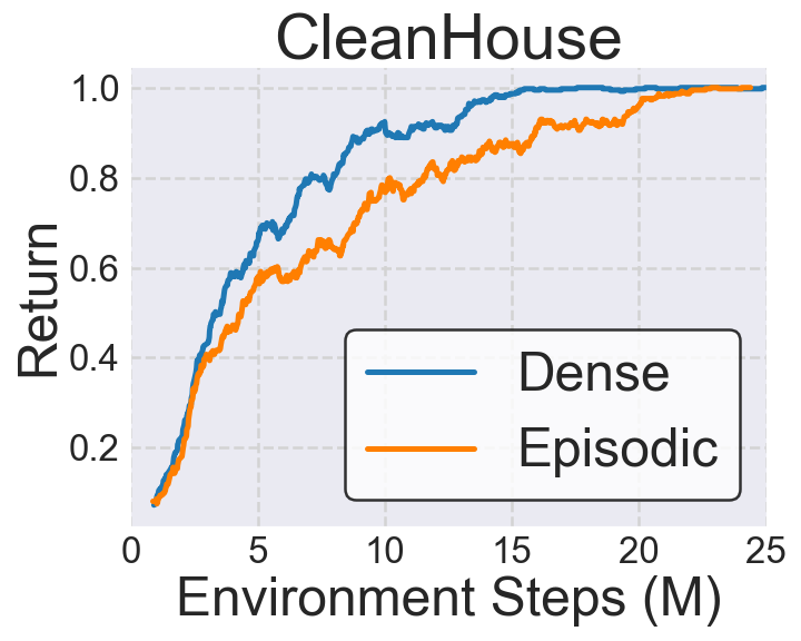
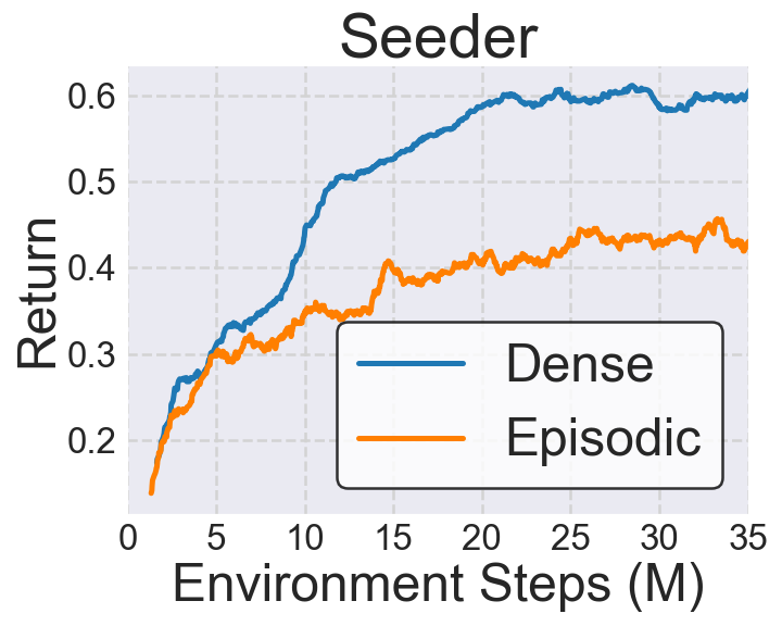
Figure 6: Learning from Episodic Reward. We compare learning from dense and episodic rewards in CleanHouse and Seeder. Learning from dense rewards achieves better sample efficiency in both tasks, which is made possible by the hierarchical design of our proposed framework.

5.4.3   Learning from Episodic Reward

We design our framework to synthesize a sequence of programs, allowing for accurately rewarding correct programs and penalizing wrong programs (i.e., better credit assignment) with dense rewards. In this section, we design experiments to investigate the effectiveness of this design. To this end, instead of receiving a reward for executing each program (i.e., dense) in the environment, we modify CleanHouse and Seeder so that they only return cumulative rewards after all $|H|$ programs have been executed (i.e., episodic). The learning performance is shown in Figure 6, demonstrating that learning from dense rewards yields better sample efficiency compared to learning from episodic rewards. This performance gain is made possible by the hierarchical design of HPRL, which can better deal with credit assignment. In contrast, LEAPS (Trivedi et al., 2021) is fundamentally limited to learning from episodic rewards.

6 Conclusion

We propose a hierarchical programmatic reinforcement learning framework (HPRL), which re-formulates solving a reinforcement learning task as synthesizing a task-solving program that can be executed to interact with the environment and maximize the return. Specifically, we first learn a program embedding space that continuously parameterizes a diverse set of programs generated based on our proposed program generation procedure. Then, we train a meta-policy, whose action space is the learned program embedding space, to produce a series of programs (i.e., predict a series of actions) to yield a composed task-solving program. Experimental results in the Karel domain demonstrate that HPRL consistently outperforms baselines by large margins. Ablation studies justify our design choices, including the RL algorithms for learning the meta-policy and the dimensionality of the program embedding space. Additional experimental results confirm the two fundamental limitations of LEAPS (Trivedi et al., 2021) and attribute the superior performance of HPRL to addressing these limitations.

Appendix

Appendix A Discussion

A.1 Synthesizing Programs with Large-Language Models

Recently, leveraging large-language models (LLM) for program generation tasks has received increasing attention. For example, OpenAI Codex (Chen et al., 2021), AlphaCode (Li et al., 2022), and related works (Chen et al., 2023; Poesia et al., 2022; Sun et al., 2020b; Jain et al., 2022) aim to produce Python/C++ code from natural language descriptions. In contrast, our goal is to synthesize programs that describe the behaviors of learning agents from rewards.

On the other hand, Liang et al. (2022) utilize LLMs to generate behavioral instructions given task-oriented prompts. However, their problem formulation involves human interventions to provide task-specific prompts, which significantly deviates from our problem formulation, which is to synthesize task-solving programs purely based on rewards automatically.

Lastly, fine-tuning LLMs trained on code, such as CodeT5 (Wang et al., 2021) and CodeT5+ (Wang et al., 2023) models, on Karel programs and leveraging its embedding space as the action space is another promising way to further enhance the performance of the proposed method.

A.2 Limitations

Karel Domain DSL. In this work, we choose the Karel DSL (Figure 1) due to its popularity among prior works (Bunel et al., 2018; Shin et al., 2018; Sun et al., 2018; Chen et al., 2019; Trivedi et al., 2021) and the expressiveness of the behavioral description for the agent. Incorporating the proposed HPRL framework for synthesizing programs with a more general DSL is worth further exploring.

Deterministic Environments. The Karel domain features a deterministic environment, where any action has a single guaranteed effect without the possibility of failure or uncertainty. Designing a DSL and a program synthesis framework that can synthesize task-solving programs in stochastic environments is another promising research direction.

Appendix B Method Details

The details of each method are described in this section.

B.1 HPRL

The overall framework of HPRL consists of two parts: the pre-trained decoder, as mentioned in Section 4.1, and the meta-policy described in Section 4.3. The decoder is constructed with a one-layer unidirectional GRU, where the hidden size and input size are set to 256. Additionally, we employ a compression decoder to further compress the latent program space. This is achieved by using a fully-connected linear neural network with an output dimension of 256 and a latent embedding dimension of $[16,32,64,128]$. Please note that the VAE with 256-dimensions program embedding space does not include the fully connected linear neural network. The meta-policy neural network consists of a CNN neural network as a state feature extractor and a fully-connected linear layer for the action and value branch. The CNN neural network includes two convolutional layers. The filter size of the first convolutional layer is $32$ with $4$ channels, and the filter size of the second convolutional layer is $32$ with $2$ channels. The output of the state embedding is flattened into a vector of the same size as the output action vector.

B.2 DRL

The DRL method implements a deep neural network trained using the Proximal Policy Optimization (PPO) algorithm for $2M$ time steps. It learns a policy that takes raw states (grids) from the Karel environment as input and predicts the next action. The raw state is represented by a binary tensor that reflects the state of each grid.

B.3 DRL-abs

DRL-abs utilizes a deep neural network with a recurrent policy and is trained using the PPO algorithm, which has demonstrated better performance compared to the Soft Actor-Critic (SAC) algorithm. It is also trained for $2M$ time steps. Instead of using the raw states (grids) of Karel, it takes abstract states as input. These abstract states are represented by a binary vector that encompasses all returned values of perceptions of the current state, e.g., [frontIsClear() == True, leftIsClear() == False, rightIsClear() == True, markerPresent() == False, noMarkersPresent() == True].

B.4 VIPER

VIPER is a programmatic RL framework proposed by Bastani et al. (2018) that utilizes a decision tree to imitate the behavior of a given neural network teacher policy. Bastani et al. (2018) utilizes the best DRL policy networks as its teacher policy. While VIPER lacks the ability to synthesize looping behaviors, it can be effectively employed for evaluating other approaches that utilize a program embedding space to synthesize more complex programs.

B.5 LEAPS

LEAPS is a programmatic RL framework introduced by Trivedi et al. (2021). The training framework of LEAPS consists of two stages. In the first stage, a model with an encoder-decoder architecture is trained to learn a continuous program embedding space. In the second stage, the Cross-Entropy Method (Rubinstein, 1997) is utilized to search through the learned program embedding space and optimize the program policy for each task.

B.6 LEAPS-ours

LEAPS-ours utilizes the same framework as LEAPS but is trained on our proposed dataset while learning a program embedding space.

Appendix C Problem Set Details

C.1 Karel Problem Set Details

The Karel problem set introduced in (Trivedi et al., 2021) consists of six different tasks: StairClimber, FourCorner, TopOff, Maze, CleanHouse and Harvester. The performance of the policy networks is measured by averaging the rewards obtained from 10 randomly generated initial configurations of the environment. All experiments are conducted on an $8\times 8$ grid, except for the CleanHouse task. Figure 7 visualizes one of the random initial configurations and its ideal end state for each Karel task.

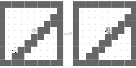
(a) StairClimber

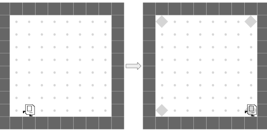
(b) fourCorner

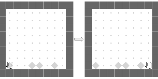
(c) TopOff

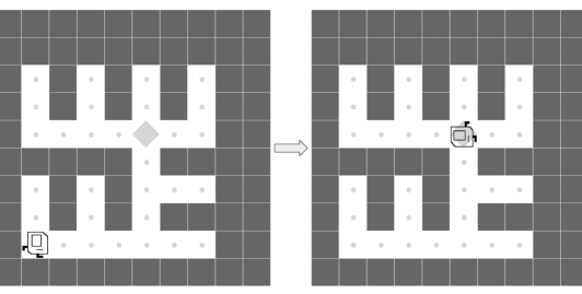
(d) Maze

(e) Harvester

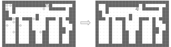
(f) CleanHouse

Figure 7: Illustrations of the initial and desired final state of each task in the Karel Problem set introduced in by Trivedi et al. (2021). Note that these illustrations are from (Trivedi et al., 2021). The position of markers, walls, and agent’s position are randomly set according to the configurations of each tasks. More details are provided in Section C.1.

StairClimber. In this task, the agent is asked to move along the stair to reach the marked grid. The initial location of the agent and the marker is randomized near the stair, with the marker placed on the higher end. The reward is defined as $1$ if the agent successfully reaches the marked grid and $0$ otherwise.

FourCorner. The goal of the agent in this task is to place a marker on each corner of the grid to earn the reward. If any marker is placed in the wrong location, the reward is $0$. The initial position of the agent is randomized near the wall. The reward is calculated by multiplying the number of correctly placed markers by $0.25$.

TopOff. In this task, the agent is asked to place markers on marked grids and reach the rightmost grid of the bottom row. The reward is defined as the consecutive correct states of the last rows until the agent puts a marker on an empty location or does not place a marker on a marked grid. If the agent successfully reaches the rightmost grid of the last row, a bonus reward is granted. The agent is always initiated on the leftmost grid of the bottom row, facing east, while the locations of markers in the last row are randomized.

Maze. In this task, the agent has to navigate to reach the marked destination. The locations of markers and the agent, as well as the configuration of the maze, are randomized. The reward is $1$ if the agent successfully reaches the marked grid or otherwise $0$.

CleanHouse. There is some garbage (markers) scattered around the apartment, and the agent is asked to clean them up. The agent’s objective is to collect as many markers as possible on the grid. The apartment is represented by a 14x22 grid. While the agent’s location remains fixed, the positions of the markers are randomized. The reward is calculated by dividing the number of markers collected by the total number of markers in the initial Karel state.

Harvester. The goal is to collect more markers on the grid, with markers appearing in all grids in the initial Karel environment. The reward is defined as the number of collected markers divided by the total markers in the initial state.

C.2 Karel-Hard Problem Set Details

Since all the tasks in the original Karel benchmark are well-solved by our method, we proposed a newly designed Karel-Hard benchmark to further evaluate the capability of HPRL. We define the state transition functions and reward functions for DoorKey, OneStroke, Seeder, and Snake based on Karel states. Each task includes more constraints and more complex structures, e.g., two-phase structure for DoorKey, the restriction of no revisiting for OneStroke.

The performance of the policy networks is measured by averaging the rewards of 10 random environment initial configurations. The range of cumulative reward in all Karel-Hard tasks is [$0.0,1.0$]. Figure 8 visualizes one of the random initial configurations and its ideal end state for each Karel-Hard task.

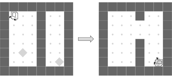
(a) DoorKey

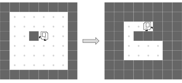
(b) OneStroke

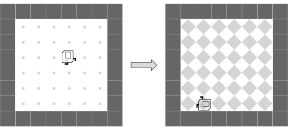
(c) Seeder

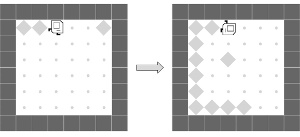
(d) Snake

Figure 8: Illustrations of the initial and final state of each task in the proposed Karel-Hard Problem Set. The position of markers, walls, and agent’s position are randomly set according to the configurations of each tasks. More details are provided in Section C.2.

DoorKey. An $8\times 8$ grid is split into two areas: a $6\times 3$ left chamber and a $6\times 2$ right chamber. The two chambers are unconnected in the beginning. The agent has to pick up the marker in the left chamber to unlock the door, and then get into the right chamber to place the marker on the top of the target(marker). The initial location of the agent, the key(marker) in the left room and the target(marker) in the right room are randomly initialized. The reward is defined as $0.5$ for picking up the key and the remaining $0.5$ for placing the marker on the marked grid.

OneStroke. The goal is to make the agent traverse all grids without revisiting. The visited grids will become a wall and the episode will terminate if the agent hits the wall. The reward is defined as the number of grids visited divided by the total empty grids in the initial Karel environment. The initial location of the agent is randomized.

Seeder. The goal is to put markers on each grid in the Karel environment. The episode will end if markers are repeatedly placed. The reward is defined as the number of markers placed divided by the total number of empty grids in the initial Karel environment.

Snake. In this task, the agent acts as the head of the snake, and the goal is to eat (i.e., pass through) as much food (markers) as possible without hitting its body. There is always exactly one marker existing in the environment until $20$ markers have been eaten. Once the agent passes a marker, the snake’s body length will increase by $1$, and a new marker will appear at another position in the environment. The reward is defined as the number of markers eaten divided by $20$.

Appendix D Hyperparameters and Settings

D.1 LEAPS

Following the setting of LEAPS(Trivedi et al., 2021), we experimented with sets of hyperparameters when searching the program embedding space to optimize the reward for both LEAPS and LEAPS-ours. The LEAPS settings are described in Table LABEL:table:karel_hard_setting and Table LABEL:table:recon_setting. S, $\sigma$, # Elites, Exp Decay and $D_{I}$ represent population size, standard deviation, percentage of population elites, exponential $\sigma$ decay and initial distribution, respectively.

Karel-Hard tasks

Table 5: LEAPS experiment settings on Karel-Hard tasks.

LEAPS	S	$\sigma$	$\#$ Elites	Exp Decay	$D_{I}$
DoorKey	32	0.25	0.1	False	$N(0,0.1I_{d})$
OneStroke	64	0.5	0.05	True	$N(1,0)$
Seeder	32	0.25	0.1	False	$N(0,0.1I_{d})$
Snake	32	0.25	0.2	False	$N(0,I_{d})$

Reconstruction tasks

Table 6: LEAPS experiment settings on Program Reconstruction tasks.

LEAPS	S	$\sigma$	$\#$ Elites	Exp Decay	$D_{I}$
Len 25	32	0.5	0.05	True	$N(0,I_{d})$
Len 50	32	0.5	0.2	True	$N(0,0.1I_{d})$
Len 75	64	0.5	0.05	True	$N(0,0.1I_{d})$
Len 100	64	0.5	0.1	True	$N(0,0.1I_{d})$

D.2 LEAPS-ours

Karel tasks

Table 7: LEAPS-ours experiment settings on Karel tasks.

LEAPS-ours	S	$\sigma$	# Elites	Exp Decay	$D_{I}$
StairClimber	32	0.5	0.05	True	$N(0,0.1I_{d})$
FourCorners	32	0.5	0.1	True	$N(1,0)$
TopOff	64	0.25	0.05	True	$N(0,0.1I_{d})$
Maze	64	0.1	0.2	False	$N(1,0)$
CleanHouse	64	0.5	0.05	True	$N(1,0)$
Harvester	64	0.5	0.05	True	$N(1,0)$

Karel-Hard tasks

Table 8: LEAPS-ours experiment settings on Karel-Hard tasks.

LEAPS-ours	S	$\sigma$	# Elites	Exp Decay	$D_{I}$
DoorKey	64	0.5	0.2	True	$N(1,0)$
OneStroke	64	0.5	0.05	True	$N(1,0)$
Seeder	64	0.5	0.05	True	$N(0,0.1,I_{d})$
Snake	32	0.25	0.05	False	$N(0,0.1,I_{d})$

D.3 HPRL

Pretraining VAE

Table 9: Hyperparameters of VAE Pretraining

Parameter	Value/Setting
Latent Embedding Size	64
GRU Hidden Layer Size	256
# GRU Layer for Encoder/Decoder	1
Batch Size	256
Nonlinearity	Tanh
Learning Rate	0.001
Latent Loss Coefficient($\beta$)	0.1

RL training on Meta Policies

The Hyperparameters for HPRL-PPO and HPRL-SAC training are reported in Table 10. For each task, we test on 5 different random seeds and take the average to measure the performance.

Table 10: Hyperparameters of HPRL-PPO and HPRL-SAC Training

Training Settings	SAC	PPO
Max # Subprogram	5	5
Max Subprogram Length	40	40
Batch Size	1024	256
Specific Parameters	Init. Temperature: 0.0002 Actor Update Frequency: 200 Critic Target Update Frequency: 200 Num Seed Steps: 20000 Replay Buffer Size: 5M Training Steps: 25M Alpha Learning Rate: 0.0001 Actor Learning Rate: 0.0001 Critic Learning Rate: 0.00001 $\beta$: [0.9, 0.999] Critic $\tau$: 0.005 Number of parallel actors: 16 Discount factor: 0.99 Q-critic Hidden Dimension: 16	Learning Rate: 0.00005 Entropy Coefficient: 0.1 Rollout Size: 12800 Eps: 0.00001 $\alpha$: 0.99 $\gamma$: 0.99 Use GAE: True GAE lambda: 0.95 Value Loss Coefficient: 0.5 Clip Param: 0.2 Max grad. norm.: 0.5 Number of mini-batches: 10 Update Epochs: 3 Training Steps: 25M

Appendix E The Karel Program Datasets Generation

Table 11: The statistical distribution of programs containing each token in our generated dataset.

	IFELSE	IF	WHILE	REPEAT
Our Dataset	41%	47%	54%	22%

The Karel program dataset used in this work includes $1$ million program sequences, with $85\%$ as the training dataset and $15\%$ as the evaluation dataset. In addition to sequences of program tokens, the Karel program dataset also includes execution demonstrations (e.g., state transition and action sequence) of each program in the dataset, which can be used for the latent behavior reconstruction loss described in Section 4.1.

To further improve the data quality, we added some heuristic rules while selecting data to filter out the programs with repetitive or offsetting behavior. The unwanted programs that we drop while collecting data are mainly determined by the following rules:

• Contradictory Primitive Actions: turnLeft followed by turnRight, pickMarker followed by putMarker, or vice versa.

• Meaningless Programs: end_state == start_state after program execution

• Repetitive behaviors: a program which has the longest common subsequence of tokens longer than 9

We further analyze the distribution of the generated program sequences based on the control flow (e.g., IF, IFELSE) and loop command (e.g., WHILE, REPEAT). The statistical probabilities of programs containing control flow or loop commands are listed in Table 11. Results show that more than 40% of the programs in the collected program sequences contain at least one of the control of loop commands, ensuring the diversity of the generated programs.

StairClimber

LEAPS

⬇

DEF run m(

WHILE c( noMarkersPresent c) w(

turnRight

move

w)

WHILE c( rightIsClear c) w(

turnLeft

w)

m)

LEAPS-ours

⬇

DEF run m(

turnRight

turnRight

WHILE c( noMarkersPresent c) w(

turnRight

move

w)

m)

HPRL-PPO

⬇

DEF run m(

WHILE c( noMarkersPresent c) w(

turnRight

move

turnRight

move

w)

m)

TopOff

LEAPS

⬇

DEF run m(

WHILE c( noMarkersPresent c) w(

move

w)

putMarker

move

WHILE c( not c( markersPresent c) c) w(

move

w)

putMarker

move

WHILE c( not c( markersPresent c) c) w(

move

w)

putMarker

move

turnRight

turnRight

turnRight

turnRight

turnRight

turnRight

turnRight

turnRight

m)

LEAPS-ours

⬇

DEF run m(

WHILE c( not c( rightIsClear c) c) w(

WHILE c( not c( markersPresent c) c) w(

move

w)

putMarker

move

w)

WHILE c( not c( rightIsClear c) c) w(

pickMarker

w)

m)

HPRL-PPO

⬇

DEF run m(

REPEAT R=5 r(

move

WHILE c( noMarkersPresent c) w(

move

w)

putMarker

r)

m)

CleanHouse

LEAPS

⬇

DEF run m(

WHILE c( noMarkersPresent c) w(

turnRight

move

move

turnLeft

turnRight

pickMarker

w)

turnLeft

turnRight

m)

LEAPS-ours

⬇

DEF run m(

move

WHILE c( noMarkersPresent c) w(

turnRight

move

WHILE c( frontIsClear c) w(

move

pickMarker

w)

w)

m)

HPRL-PPO

⬇

DEF run m(

WHILE c( noMarkersPresent c) w(

turnRight

move

pickMarker

pickMarker

w)

m)

DEF run m(

WHILE c( noMarkersPresent c) w(

turnRight

move

pickMarker

pickMarker

w)

m)

DEF run m(

WHILE c( noMarkersPresent c) w(

turnRight

move

pickMarker

pickMarker

w)

m)

DEF run m(

WHILE c( noMarkersPresent c) w(

turnRight

move

pickMarker

pickMarker

w)

m)

Figure 10: Example programs on Karel tasks: StairClimber, TopOff and CleanHouse. The programs with best rewards out of all random seeds are shown.

FourCorner

LEAPS

⬇

DEF run m(

turnRight

move

turnRight

turnRight

turnRight

WHILE c( frontIsClear c) w(

move

w)

turnRight

putMarker

WHILE c( frontIsClear c) w(

move

w)

turnRight

putMarker

WHILE c( frontIsClear c) w(

move

w)

turnRight

putMarker

WHILE c( frontIsClear c) w(

move

w)

turnRight

putMarker

m)

LEAPS-ours

⬇

DEF run m(

REPEAT R=5 r(

WHILE c( frontIsClear c) w(

move

w)

IFELSE c( not c( rightIsClear c) c) i(

turnLeft

putMarker

i)

ELSE e(

putMarker

e)

r)

m)

HPRL-PPO

⬇

DEF run m(

move

WHILE c( frontIsClear c) w(

move

w)

putMarker

turnLeft

m)

DEF run m(

move

WHILE c( frontIsClear c) w(

move

w)

putMarker

turnLeft

m)

DEF run m(

move

WHILE c( frontIsClear c) w(

move

w)

putMarker

turnLeft

m)

DEF run m(

move

WHILE c( frontIsClear c) w(

move

w)

putMarker

turnLeft

m)

Maze

LEAPS

⬇

DEF run m(

IF c( frontIsClear c) i(

turnLeft

i)

WHILE c( noMarkersPresent c) w(

turnRight

move

w)

m)

LEAPS-ours

⬇

DEF run m(

WHILE c( noMarkersPresent c) w(

turnRight

move

w)

turnRight

turnRight

turnRight

m)

HPRL-PPO

⬇

DEF run m(

WHILE c( noMarkersPresent c) w(

turnRight

move

w)

WHILE c( noMarkersPresent c) w(

turnRight

move

w)

m)

Figure 12: Example programs on Karel tasks: FourCorner and Maze. The programs with best rewards out of all random seeds are shown.

Harvester

LEAPS

⬇

DEF run m(

turnLeft

turnLeft

pickMarker

move

pickMarker

pickMarker

move

pickMarker

move

pickMarker

move

pickMarker

move

turnLeft

pickMarker

move

pickMarker

move

pickMarker

move

pickMarker

move

turnLeft

pickMarker

move

pickMarker

move

pickMarker

move

pickMarker

move

turnLeft

pickMarker

move

pickMarker

move

pickMarker

move

m)

LEAPS-ours

⬇

DEF run m(

WHILE c( leftIsClear c) w(

REPEAT R=4 r(

pickMarker

move

r)

turnLeft

pickMarker

move

turnLeft

pickMarker

move

w)

turnLeft

pickMarker

turnLeft

m)

HPRL-PPO

⬇

DEF run m(

REPEAT R=4 r(

REPEAT R=4 r(

pickMarker

turnRight

move

pickMarker

turnRight

move

pickMarker

move

pickMarker

move

r)

turnRight

pickMarker

move

pickMarker

move

pickMarker

move

r)

m)

Figure 14: Example programs on Karel tasks: Harvester. The programs with best rewards out of all random seeds are shown.

DoorKey

LEAPS

⬇

DEF run m(

move

turnRight

putMarker

pickMarker

move

WHILE c( leftIsClear c) w(

pickMarker

move

w)

m)

LEAPS-ours

⬇

DEF run m(

WHILE c( rightIsClear c) w(

turnRight

pickMarker

turnLeft

pickMarker

pickMarker

pickMarker

pickMarker

move

turnLeft

move

w)

m)

HPRL-PPO

⬇

DEF run m(

REPEAT R=4 r(

REPEAT R=4 r( turnRight move pickMarker move pickMarker move r)

pickMarker move r)

m)

DEF run m(

REPEAT R=5 r(

turnRight move

REPEAT R=5 r( move r)

move pickMarker move

r)

m)

DEF run m(

REPEAT R=4 r(

REPEAT R=4 r(

turnRight move

REPEAT R=3 r(

move pickMarker

move pickMarker r)

r)

r)

m)

DEF run m(

REPEAT R=4 r(

REPEAT R=4 r(

turnRight move

pickMarker move

pickMarker

REPEAT R=2 r(

pickMarker move

pickMarker pickMarker r)

r)

r)

m)

DEF run m(

REPEAT R=4 r(

turnRight

REPEAT R=4 r(

turnRight move move

pickMarker move

r)

move pickMarker move

r)

move pickMarker

m)

Figure 16: Example programs on Karel-Hard tasks: DoorKey. The programs with best rewards out of all random seeds are shown.

OneStroke

LEAPS

⬇

DEF run m(

REPEAT R=9 r(

turnRight

turnRight

WHILE c( frontIsClear c) w(

move

w)

turnRight

WHILE c( frontIsClear c) w(

move

w)

r)

turnRight

m)

LEAPS-ours

⬇

DEF run m(

turnRight

WHILE c( frontIsClear c) w(

WHILE c( frontIsClear c) w(

WHILE c( frontIsClear c) w(

WHILE c( frontIsClear c) w(

move

w)

turnRight

w)

turnRight

w)

turnRight

w)

turnRight

m)

HPRL-PPO

⬇

DEF run m(

WHILE c( frontIsClear c) w( move w) turnRight

WHILE c( frontIsClear c) w( move w) turnRight

WHILE c( frontIsClear c) w( move w) turnRight

m)

DEF run m(

WHILE c( frontIsClear c) w( move w) turnRight

WHILE c( frontIsClear c) w( move w) turnRight

WHILE c( frontIsClear c) w( move w) turnRight

m)

DEF run m(

WHILE c( frontIsClear c) w( move w) turnRight

WHILE c( frontIsClear c) w( move w) turnRight

WHILE c( frontIsClear c) w( move w) turnRight

WHILE c( frontIsClear c) w( move w) turnRight

m)

DEF run m(

WHILE c( frontIsClear c) w( move w) turnRight

WHILE c( frontIsClear c) w( move w) turnRight

WHILE c( frontIsClear c) w( move w) turnRight

m)

Figure 18: Example programs on Karel-Hard tasks: OneStroke. The programs with best rewards out of all random seeds are shown.

Seeder

LEAPS

⬇

DEF run m(

WHILE c( noMarkersPresent c) w(

turnRight

putMarker

move

move

w)

turnRight

turnRight

turnRight

turnRight

turnRight

turnRight

turnRight

turnRight

m)

LEAPS-ours

⬇

DEF run m(

WHILE c( noMarkersPresent c) w(

putMarker

move

turnRight

move

w)

turnRight

turnRight

turnRight

turnRight

turnRight

turnRight

turnRight

turnRight

m)

HPRL-PPO

⬇

DEF run m(

putMarker move

putMarker move

putMarker move

putMarker move

putMarker move

turnRight move

m)

DEF run m(

putMarker move

putMarker move

putMarker move

putMarker move

putMarker move

turnRight move

putMarker move

m)

DEF run m(

putMarker move

putMarker move

putMarker move

putMarker move

turnRight move

putMarker move

turnRight move

m)

DEF run m(

putMarker move

putMarker move

putMarker move

putMarker move

turnRight move

putMarker move

turnRight move

DEF run m(

putMarker move

putMarker move

putMarker move

putMarker move

turnRight move

putMarker move

turnRight move

m)

Snake

LEAPS

⬇

DEF run m(

turnRight

turnLeft

pickMarker

move

move

move

WHILE c( rightIsClear c) w(

turnLeft

move

move

w)

turnLeft

turnLeft

turnLeft

turnLeft

m)

LEAPS-ours

⬇

DEF run m(

move

turnRight

pickMarker

pickMarker

WHILE c( rightIsClear c) w(

turnLeft

move

move

w)

turnRight

move

move

move

m)

HPRL-PPO

⬇

DEF run m(

move

WHILE c( noMarkersPresent c) w(

move

move

turnLeft

w)

move

turnLeft

m)

DEF run m(

move

WHILE c( noMarkersPresent c) w(

move

move

turnLeft

w)

m)

DEF run m(

move

WHILE c( noMarkersPresent c) w(

move

move

turnLeft

w)

move

turnLeft

m)

Figure 20: Example programs on Karel-Hard tasks: Seeder and Snake. The programs with best rewards out of all random seeds are shown.

Appendix F Evaluation Metric for Learning to Synthesize Out-of-distributional Programs

Measure the Performance. To measure the performance of programs synthesized by different methods, we first collect and execute each target program, yielding a target state sequence $\tau_{target}=[s_{1},s_{2},\dotsc,s_{T_{target}}]$. Then, we reset the Karel environment to the initial state $s_{1}$. For our proposed framework, we synthesize a sequence of programs with the following procedure and optimize a program reconstruction reward to match the target program. As described in Section 4.3, at each macro training time step $n,1\leq n\leq|H|$, we collect the state sequence $\tau_{\mathcal{P}}=[s^{\mathcal{P}}_{1},s^{\mathcal{P}}_{2},\dotsc,s^{\mathcal{P}}_{T_{\mathcal{P}}}]$ from the executing of task-solving program $\mathcal{P}=\langle\rho_{i}|i=1,..,n\rangle$, and calculate the program reconstruction reward $r^{n}=1-\mathcal{D}(\tau_{target},\tau_{\mathcal{P}})$ where $\mathcal{D}$ is the normalized Levenshtein distance. For executing the programs synthesized by LEAPS and LEAPS-ours, we simply start executing programs after resetting the Karel environment to the initial state $s_{1}$ and calculating the return.

Appendix G Synthesized Programs

In this section, we provide qualitative results (i.e., synthesized programs) of our proposed framework (HPRL-PPO), LEAPS, and LEAPS-ours. The programs synthesized for the tasks in the Karel problem set are shown in Figure 10 (StairClimber, TopOff, and CleanHouse), Figure 12 (FourCorner, Maze), and Figure 14 (Harvester). The programs synthesized for the tasks in the Karel-Hard problem set are shown in Figure 16 (DoorKey), Figure 18(OneStroke), and Figure 20 (Seeder and Snake).

References

- Bacon et al. (2017) Bacon, P.-L., Harb, J., and Precup, D. The option-critic architecture. In Association for the Advancement of Artificial Intelligence, 2017.
- Balog et al. (2017) Balog, M., Gaunt, A. L., Brockschmidt, M., Nowozin, S., and Tarlow, D. Deepcoder: Learning to write programs. In International Conference on Learning Representations, 2017.
- Barto & Mahadevan (2003) Barto, A. G. and Mahadevan, S. Recent advances in hierarchical reinforcement learning. Discrete Event Dynamic Systems, 2003.
- Bastani et al. (2018) Bastani, O., Pu, Y., and Solar-Lezama, A. Verifiable reinforcement learning via policy extraction. In Neural Information Processing Systems, 2018.
- Bunel et al. (2018) Bunel, R. R., Hausknecht, M., Devlin, J., Singh, R., and Kohli, P. Leveraging grammar and reinforcement learning for neural program synthesis. In International Conference on Learning Representations, 2018.
- Chen et al. (2021) Chen, M., Tworek, J., Jun, H., Yuan, Q., Pinto, H. P. d. O., Kaplan, J., Edwards, H., Burda, Y., Joseph, N., Brockman, G., Ray, A., Puri, R., Krueger, G., Petrov, M., Khlaaf, H., Sastry, G., Mishkin, P., Chan, B., Gray, S., Ryder, N., Pavlov, M., Power, A., Kaiser, L., Bavarian, M., Winter, C., Tillet, P., Such, F. P., Cummings, D., Plappert, M., Chantzis, F., Barnes, E., Herbert-Voss, A., Guss, W. H., Nichol, A., Paino, A., Tezak, N., Tang, J., Babuschkin, I., Balaji, S., Jain, S., Saunders, W., Hesse, C., Carr, A. N., Leike, J., Achiam, J., Misra, V., Morikawa, E., Radford, A., Knight, M., Brundage, M., Murati, M., Mayer, K., Welinder, P., McGrew, B., Amodei, D., McCandlish, S., Sutskever, I., and Zaremba, W. Evaluating large language models trained on code. arXiv preprint arXiv:2107.03374, 2021.
- Chen et al. (2019) Chen, X., Liu, C., and Song, D. Execution-guided neural program synthesis. In International Conference on Learning Representations, 2019.
- Chen et al. (2023) Chen, X., Lin, M., Schärli, N., and Zhou, D. Teaching large language models to self-debug. arXiv preprint arXiv:2304.05128, 2023.
- Cho et al. (2014) Cho, K., van Merrienboer, B., Bahdanau, D., and Bengio, Y. On the properties of neural machine translation: Encoder-decoder approaches, 2014.
- Choi & Langley (2005) Choi, D. and Langley, P. Learning teleoreactive logic programs from problem solving. In International Conference on Inductive Logic Programming, 2005.
- Cobbe et al. (2019) Cobbe, K., Klimov, O., Hesse, C., Kim, T., and Schulman, J. Quantifying generalization in reinforcement learning. In International Conference on Machine Learning, 2019.
- Devlin et al. (2017) Devlin, J., Uesato, J., Bhupatiraju, S., Singh, R., Mohamed, A.-r., and Kohli, P. Robustfill: Neural program learning under noisy i/o. In International Conference on Machine Learning, 2017.
- Dong et al. (2019) Dong, H., Mao, J., Lin, T., Wang, C., Li, L., and Zhou, D. Neural logic machines. In International Conference on Learning Representations, 2019.
- Ellis et al. (2020) Ellis, K., Wong, C., Nye, M., Sable-Meyer, M., Cary, L., Morales, L., Hewitt, L., Solar-Lezama, A., and Tenenbaum, J. B. Dreamcoder: Growing generalizable, interpretable knowledge with wake-sleep bayesian program learning. arXiv preprint arXiv:2006.08381, 2020.
- Ellis et al. (2021) Ellis, K., Wong, C., Nye, M., Sablé-Meyer, M., Morales, L., Hewitt, L., Cary, L., Solar-Lezama, A., and Tenenbaum, J. B. Dreamcoder: Bootstrapping inductive program synthesis with wake-sleep library learning. In SIGPLAN International Conference on Programming Language Design and Implementation 2021, 2021.
- Fukushima & Miyake (1982) Fukushima, K. and Miyake, S. Neocognitron: A self-organizing neural network model for a mechanism of visual pattern recognition. In Competition and Cooperation in Neural Nets: Proceedings of the US-Japan Joint Seminar, 1982.
- Graves et al. (2014) Graves, A., Wayne, G., and Danihelka, I. Neural turing machines. arXiv preprint arXiv:1410.5401, 2014.
- Gu et al. (2017) Gu, S., Holly, E., Lillicrap, T., and Levine, S. Deep reinforcement learning for robotic manipulation with asynchronous off-policy updates. In IEEE International Conference on Robotics and Automation, 2017.
- Haarnoja et al. (2018) Haarnoja, T., Zhou, A., Abbeel, P., and Levine, S. Soft actor-critic: Off-policy maximum entropy deep reinforcement learning with a stochastic actor. In International Conference on Machine Learning, 2018.
- Higgins et al. (2016) Higgins, I., Matthey, L., Pal, A., Burgess, C., Glorot, X., Botvinick, M., Mohamed, S., and Lerchner, A. beta-vae: Learning basic visual concepts with a constrained variational framework. In International Conference on Learning Representations, 2016.
- Hong et al. (2021) Hong, J., Dohan, D., Singh, R., Sutton, C., and Zaheer, M. Latent programmer: Discrete latent codes for program synthesis. In International Conference on Machine Learning, 2021.
- Ibarz et al. (2021) Ibarz, J., Tan, J., Finn, C., Kalakrishnan, M., Pastor, P., and Levine, S. How to train your robot with deep reinforcement learning: lessons we have learned. The International Journal of Robotics Research, 2021.
- Inala et al. (2020) Inala, J. P., Bastani, O., Tavares, Z., and Solar-Lezama, A. Synthesizing programmatic policies that inductively generalize. In International Conference on Learning Representations, 2020.
- Jain et al. (2022) Jain, N., Vaidyanath, S., Iyer, A., Natarajan, N., Parthasarathy, S., Rajamani, S., and Sharma, R. Jigsaw: Large language models meet program synthesis. In International Conference on Software Engineering, 2022.
- Krizhevsky et al. (2017) Krizhevsky, A., Sutskever, I., and Hinton, G. E. Imagenet classification with deep convolutional neural networks. Communications of the ACM, 2017.
- Landajuela et al. (2021) Landajuela, M., Petersen, B. K., Kim, S., Santiago, C. P., Glatt, R., Mundhenk, N., Pettit, J. F., and Faissol, D. Discovering symbolic policies with deep reinforcement learning. In International Conference on Machine Learning, 2021.
- Lee et al. (2019) Lee, Y., Sun, S.-H., Somasundaram, S., Hu, E., and Lim, J. J. Composing complex skills by learning transition policies. In International Conference on Learning Representations, 2019.
- Lee et al. (2021) Lee, Y., Szot, A., Sun, S.-H., and Lim, J. J. Generalizable imitation learning from observation via inferring goal proximity. In Neural Information Processing Systems, 2021.
- Li et al. (2022) Li, Y., Choi, D., Chung, J., Kushman, N., Schrittwieser, J., Leblond, R., Eccles, T., Keeling, J., Gimeno, F., Lago, A. D., Hubert, T., Choy, P., d’Autume, C. d. M., Babuschkin, I., Chen, X., Huang, P.-S., Welbl, J., Gowal, S., Cherepanov, A., Molloy, J., Mankowitz, D. J., Robson, E. S., Kohli, P., de Freitas, N., Kavukcuoglu, K., and Vinyals, O. Competition-level code generation with alphacode. Science, 2022.
- Liang et al. (2022) Liang, J., Huang, W., Xia, F., Xu, P., Hausman, K., Ichter, B., Florence, P., and Zeng, A. Code as policies: Language model programs for embodied control. In arXiv preprint arXiv:2209.07753, 2022.
- Liao et al. (2019) Liao, Y.-H., Puig, X., Boben, M., Torralba, A., and Fidler, S. Synthesizing environment-aware activities via activity sketches. In IEEE Conference on Computer Vision and Pattern Recognition, 2019.
- Lin et al. (2018) Lin, X. V., Wang, C., Zettlemoyer, L., and Ernst, M. D. Nl2bash: A corpus and semantic parser for natural language interface to the linux operating system. In International Conference on Language Resources and Evaluation, 2018.
- Lipton (2016) Lipton, Z. C. The mythos of model interpretability. In ICML Workshop on Human Interpretability in Machine Learning, 2016.
- Liu et al. (2022) Liu, G.-T., Lin, G.-Y., and Cheng, P.-J. Improving generalization with cross-state behavior matching in deep reinforcement learning. In Autonomous Agents and Multiagent Systems, 2022.
- Liu et al. (2019) Liu, Y., Wu, J., Wu, Z., Ritchie, D., Freeman, W. T., and Tenenbaum, J. B. Learning to describe scenes with programs. In International Conference on Learning Representations, 2019.
- Pattis (1981) Pattis, R. E. Karel the robot: a gentle introduction to the art of programming. John Wiley & Sons, Inc., 1981.
- Poesia et al. (2022) Poesia, G., Polozov, O., Le, V., Tiwari, A., Soares, G., Meek, C., and Gulwani, S. Synchromesh: Reliable code generation from pre-trained language models. arXiv preprint arXiv:2201.11227, 2022.
- Puiutta & Veith (2020) Puiutta, E. and Veith, E. M. S. P. Explainable reinforcement learning: A survey. In Holzinger, A., Kieseberg, P., Tjoa, A. M., and Weippl, E. R. (eds.), Machine Learning and Knowledge Extraction - International Cross-Domain Conference, CD-MAKE, 2020.
- Reed & De Freitas (2016) Reed, S. and De Freitas, N. Neural programmer-interpreters. In International Conference on Learning Representations, 2016.
- Rubinstein (1997) Rubinstein, R. Y. Optimization of computer simulation models with rare events. European Journal of Operational Research, 1997.
- Schulman et al. (2017) Schulman, J., Wolski, F., Dhariwal, P., Radford, A., and Klimov, O. Proximal policy optimization algorithms. arXiv preprint arXiv:1707.06347, 2017.
- Shin et al. (2018) Shin, E. C., Polosukhin, I., and Song, D. Improving neural program synthesis with inferred execution traces. In Neural Information Processing Systems, 2018.
- Silver et al. (2016) Silver, D., Huang, A., Maddison, C. J., Guez, A., Sifre, L., Van Den Driessche, G., Schrittwieser, J., Antonoglou, I., Panneershelvam, V., Lanctot, M., et al. Mastering the game of go with deep neural networks and tree search. Nature, 2016.
- Silver et al. (2017) Silver, D., Schrittwieser, J., Simonyan, K., Antonoglou, I., Huang, A., Guez, A., Hubert, T., Baker, L., Lai, M., Bolton, A., Chen, Y., Lillicrap, T., Hui, F., Sifre, L., van den Driessche, G., Graepel, T., and Hassabis, D. Mastering the game of go without human knowledge. Nature, 2017.
- Silver et al. (2020) Silver, T., Allen, K. R., Lew, A. K., Kaelbling, L. P., and Tenenbaum, J. Few-shot bayesian imitation learning with logical program policies. In Association for the Advancement of Artificial Intelligence, 2020.
- Sun et al. (2018) Sun, S.-H., Noh, H., Somasundaram, S., and Lim, J. Neural program synthesis from diverse demonstration videos. In International Conference on Machine Learning, 2018.
- Sun et al. (2020a) Sun, S.-H., Wu, T.-L., and Lim, J. J. Program guided agent. In International Conference on Learning Representations, 2020a.
- Sun et al. (2020b) Sun, Z., Zhu, Q., Xiong, Y., Sun, Y., Mou, L., and Zhang, L. Treegen: A tree-based transformer architecture for code generation. In Association for the Advancement of Artificial Intelligence, 2020b.
- Sutton et al. (1999) Sutton, R. S., Precup, D., and Singh, S. Between mdps and semi-mdps: A framework for temporal abstraction in reinforcement learning. Artificial intelligence, 1999.
- Tian et al. (2019) Tian, Y., Luo, A., Sun, X., Ellis, K., Freeman, W. T., Tenenbaum, J. B., and Wu, J. Learning to infer and execute 3d shape programs. In International Conference on Learning Representations, 2019.
- Trivedi et al. (2021) Trivedi, D., Zhang, J., Sun, S.-H., and Lim, J. J. Learning to synthesize programs as interpretable and generalizable policies. In Advances in Neural Information Processing Systems, 2021.
- Verma et al. (2018) Verma, A., Murali, V., Singh, R., Kohli, P., and Chaudhuri, S. Programmatically interpretable reinforcement learning. In International Conference on Machine Learning, 2018.
- Verma et al. (2019) Verma, A., Le, H., Yue, Y., and Chaudhuri, S. Imitation-projected programmatic reinforcement learning. In Neural Information Processing Systems, 2019.
- Vezhnevets et al. (2017) Vezhnevets, A. S., Osindero, S., Schaul, T., Heess, N., Jaderberg, M., Silver, D., and Kavukcuoglu, K. Feudal networks for hierarchical reinforcement learning. In International Conference on Machine Learning, 2017.
- Vinyals et al. (2019) Vinyals, O., Babuschkin, I., Czarnecki, W. M., Mathieu, M., Dudzik, A., Chung, J., Choi, D. H., Powell, R., Ewalds, T., Georgiev, P., et al. Grandmaster level in starcraft ii using multi-agent reinforcement learning. Nature, 2019.
- Wang et al. (2021) Wang, Y., Wang, W., Joty, S., and Hoi, S. C. Codet5: Identifier-aware unified pre-trained encoder-decoder models for code understanding and generation. In Empirical Methods in Natural Language Processing, 2021.
- Wang et al. (2023) Wang, Y., Le, H., Gotmare, A. D., Bui, N. D., Li, J., and Hoi, S. C. Codet5+: Open code large language models for code understanding and generation. arXiv preprint arXiv:2305.07922, 2023.
- Williams (1992) Williams, R. J. Simple statistical gradient-following algorithms for connectionist reinforcement learning. Machine learning, 1992.
- Winner & Veloso (2003) Winner, E. and Veloso, M. Distill: Learning domain-specific planners by example. In International Conference on Machine Learning, 2003.
- Wu et al. (2017) Wu, J., Tenenbaum, J. B., and Kohli, P. Neural scene de-rendering. In IEEE Conference on Computer Vision and Pattern Recognition, 2017.
- Wurman et al. (2022) Wurman, P. R., Barrett, S., Kawamoto, K., MacGlashan, J., Subramanian, K., Walsh, T. J., Capobianco, R., Devlic, A., Eckert, F., Fuchs, F., et al. Outracing champion gran turismo drivers with deep reinforcement learning. Nature, 2022.
- Zaremba & Sutskever (2015) Zaremba, W. and Sutskever, I. Reinforcement learning neural turing machines-revised. arXiv preprint arXiv:1505.00521, 2015.
- Zhang et al. (2018) Zhang, C., Vinyals, O., Munos, R., and Bengio, S. A study on overfitting in deep reinforcement learning. arXiv preprint arXiv:1804.06893, 2018.
- Zhong et al. (2023) Zhong, L., Lindeborg, R., Zhang, J., Lim, J. J., and Sun, S.-H. Hierarchical neural program synthesis. arXiv preprint arXiv:2303.06018, 2023.