Dirac equation in curved spacetime: the role of local Fermi velocity

Abstract

We study the motion of charge carriers in curved Dirac materials, in the presence of a local Fermi velocity. An explicit parameterization of the latter emerging quantity for a nanoscroll cylindrical geometry is also provided, together with a discussion of related physical effects and observable properties.

Keywords:

Dirac equation, graphene, local Fermi velocity, nanoscrolls.

1  Introduction

Dirac equation is one of the most relevant contributions in the history of quantum mechanics. Over the decades, its study has been conducted from different points of view [1, 2, 3], with countless applications in many areas of physics. The reformulation of the Dirac formalism in curved backgrounds is an appealing field of research due to its remarkable applications in high-energy physics, quantum field theory, analogue gravity scenarios and condensed matter.

A real, solid-state system where to observe the properties of Dirac spinorial quantum fields in a curved space is provided by graphene and other two-dimensional materials. The latter have attracted great interest because of their electronic, mechanical and optical characteristics [4, 5, 6, 7]. The analysis of the electronic structure of these special substrates has received further contributions from theoretical studies on the dynamics of Dirac particles in curved spacetime. In particular, an effective low-energy model, formally equivalent to a Dirac equation, emerges in graphene-like materials; the resulting formulation then provides a powerful tool to describe the motion of the long-wavelengths charge carriers [8, 9, 10, 11, 12, 13, 14, 15, 16, 17, 18, 19]. Furthermore, from a practical perspective, stability, flexibility and near-ballistic transport at room temperature, make Dirac materials [20] an ideal framework for many nanoscale applications [21, 22, 23, 24, 25, 26].

Curvature effects.

In the large wavelength regime [27, 28, 10], where quasiparticles wavelengths are large if compared with the honeycomb dimensions, curvature effects in Dirac materials have been extensively studied [29, 8, 30]. Intrinsic curvature deformations involve inelastic effects (usually coming from the formation of disclination-type defects), that turn out to work as potentials for pseudomagnetic fields modulated by curvature. Extrinsic curvature is an elastic effect coming from graphene sheet warping, determining a variation of the bond angles between orbitals and introducing peculiar effects in the electronic properties of the material [31, 32, 33].

Effects from intrinsic curvature have been subject of much more attention within the graphene community, the inelastic deformation giving rise to the emergence of pseudogauge fields directly affecting the carrier dynamics and the electronic properties of the sample [12]. In the following, instead, we focus on an extrinsic curvature framework, where the contributions of the pseudogauge fields are neglected and the physical properties are determined by the specific folding of the sample, expressed in terms of the related parametrization.

Local Fermi velocity.

It is well recognized that a gap formation in graphene-like systems [34, 35] suggests the inclusion of a spatially-varying Fermi velocity in the sample [36, 37, 38, 39]. Confirmations in this direction also come from spectroscopy experiments [30, 40, 41, 42]. In addition, the need for a local Fermi velocity (LFV) emerges from the electronic transport in two-dimensional strained Dirac materials [43]; the latter feature has triggered a wide range of researches [44, 45, 46, 47, 48, 49, 50].

From a theoretical point of view, the study of an effective Dirac behavior from lattice symmetry or, in a more general context, from low-energy expansion for distorted lattices in continuum approximation [51, 52] has allowed a better understanding of the correspondence between the lattice formulations and the quantum field covariant approach in curved space, justifying an emergent spatial dependence for the Fermi velocity [30]. On the other hand, the studies on heterostructures in graphene-like materials suggest that the dynamics of the charge carriers in the substrate can be described in terms of an effective Dirac model with a non-constant Fermi velocity [53]. The latter features a position dependence that can be induced, e.g., by the presence of lattice strains, by specific curved geometries producing interlayer interactions, by deposition of graphene layers on suitable substrates giving rise to local on-site potentials spoiling the original symmetry [35, 37, 40, 41, 54, 55].

A related, critical aspect in graphene-like materials is the generation of position-dependent mass (PDM) effects [56, 57, 58, 59, 60, 61, 62, 63, 64, 65, 66, 67, 68, 69]. This has led to several theoretical studies, including those on wave packet dynamics and propagation in topological materials [70, 71, 72, 73]. In the context of PDM, we are dealing with a generalized form of the Schrödinger equation, involving a set of ambiguity parameters. In this regard, von Roos [74] showed that it is possible to construct a Hermitian form for the governing Hamiltonian, whose expression depends on the above-mentioned parameters.

In this work we consider some features of electron dynamics in Dirac materials, in the long-wavelength approximation and in the presence of a non-trivial local Fermi velocity. We focus, in particular, on nanoscroll geometry. Graphene nanoscrolls are physically relevant due to their remarkable electronic, mechanical and optical properties, originating from their peculiar curved geometry [75, 76]. In this regard, we want to discuss physical observables exploiting a low-energy model with an effective Dirac equation for the charge carriers.

As we will discuss, the nanoscroll geometry is intrinsically flat: since the emerging local pseudomagnetic fields are proportional to the local Gaussian curvature [77, 78], we do not consider them in our cylindrical geometry, the associated Gaussian curvature being zero everywhere.

The paper is organized as follows. In Sect. 2, we discuss the procedure we use to parameterize the underlying curved spacetime, restricting on a set of suitable cylindrical coordinates for the related Dirac equation. In Sect. 3, we analyze the influence of the LFV on the Dirac equation, reformulating the problem in terms of modified $\gamma$-matrices. In Sect. 4, we take into account the impact of PDM in our formulation and discuss the explicit case of a graphene nanoscroll, taking into account the density of states as a simple observable and commenting on the measurement issues. Finally, in Sect. 5, we briefly summarize the obtained results.

2  Parameterizing the curved spacetime

We start recovering the coordinates of a conventional three-dimensional spacetime in cylindrical coordinates as specified in [15, 33]:

$$x^{\textsc{a}}=(t,x,y,z)\quad\Rightarrow\quad x^{\mu}=(t,\phi,z)\>,$$ (1)

having expressed the former coordinates as

$$x=r(\phi)\cos(\phi)\,,\qquad y=r(\phi)\sin(\phi)\,,\qquad z=z\,,$$ (2)

with an explicit $\phi$–dependence for the radius. Making use of the Jacobian ${J^{\textsc{a}}_{\mu}=\frac{\partial x^{\textsc{a}}}{\partial x^{\mu}}}$, we find the explicit form of the metric $g_{\mu\nu}$:

$$g_{\mu\nu}\,=\,\left(J^{\textsc{a}}_{\mu}\right)^{\textsc{\!t}}\eta_{\textsc{ab}}\>J^{\textsc{b}}_{\nu}\>=\>\operatorname{diag}\left(1,\,-f(\phi)^{2},\,-1\right)\,,$$ (3)

where the quantity $f(\phi)^{2}$ reads

$$f(\phi)^{2}=r(\phi)^{2}+r^{\prime}(\phi)^{2}\>.$$ (4)

As a result, the line element for the curved space assumes the form

$$ds^{2}=g_{\mu\nu}\,dx^{\mu}\,dx^{\nu}=dt^{2}-f(\phi)^{2}\,d\phi^{2}-dz^{2}\>.$$ (5)

The flat-space Dirac equation is defined in terms of flat $\gamma$-matrices that we can parameterize in terms of Pauli matrices as

$$\gamma_{a}=\{\sigma_{3},\,-i\,\sigma_{1},\,i\,\sigma_{2}\}\,,\qquad a=0,1,2$$ (6)

and obey the Clifford algebra

$$\{\gamma^{a},\gamma^{b}\}=2\,\eta^{ab}\,\mathds{1}\,,\qquad\quad\eta^{ab}=\begin{pmatrix}1&0\\ 0&-\mathds{1}\end{pmatrix}.$$ (7)

To derive the form of the Dirac equation in curved space, we consider a tetrad basis at each spacetime point. The $\gamma_{\mu}$ matrices for the curved background, that we label by Greek indices, are obtained by means of the vielbeins $e_{\mu}{}^{a}$:

$$\gamma_{\mu}=e_{\mu}{}^{a}\,\gamma_{a}\,,\qquad\quad e_{\mu}{}^{a}=\operatorname{diag}\left(1,\,f(\phi),\,1\right)\,,$$ (8)

where $\gamma^{\mu}=g^{\mu\nu}\,\gamma_{\nu}$ satisfy the curved space Clifford algebra

$$\{\gamma^{\mu},\gamma^{\nu}\}=2\,g^{\mu\nu}\,\mathds{1},\qquad\quad\mu=0,1,2.$$ (9)

The flat Dirac equation in the presence of an electromagnetic field $A^{a}(x)$,

$$\left[i\hbar\,\gamma^{a}\left(\partial_{a}+\frac{g}{i\hbar}\,A_{a}\right)-m\right]\Psi=0\>,$$ (10)

acquires, in the curved background, the form:

$$\left[i\hbar\,\gamma^{\mu}\left(\partial_{\mu}+\Omega_{\mu}+\frac{g}{i\hbar}A_{\mu}\right)-m\right]\Psi=0\>,$$ (11)

where $\Omega_{\mu}=\frac{1}{4}\,\omega_{\mu}{}^{ab}\,M_{ab}$ is the spin affine connection, expressed in terms of the spin connection $\omega_{\mu}{}^{ab}$ and Lorentz generators $M_{ab}=\frac{1}{2}[\gamma_{a},\gamma_{b}]$ [79, 80]. According to the tetrad postulate, the gamma matrices of the curved space are covariantly constant. Furthermore, the existence of a confining potential is crucial in the thin-layer quantization approach [81, 82].

Imposing the cylindrical symmetry of space, the spin affine connection $\Omega_{\mu}$ vanishes and (11) simplifies to

$$\left[i\hbar\,\gamma^{\mu}\left(\partial_{\mu}+\frac{g}{i\hbar}A_{\mu}\right)-m\right]\Psi=0\>,$$ (12)

having the same form of (10), but expressed in terms of the curved $\gamma^{\mu}$ matrices.

3  Impact of a local Fermi velocity

For heterostructures, the Fermi velocity becomes position-dependent [53, 83, 84]:

$$v_{\textsc{f}}\;\rightarrow\;v_{\textsc{f}}(\phi,z)\>,$$ (13)

and this also affects Dirac equation (10), that is modified as [53, 85, 86]

$$\left[i\hbar\,\Gamma^{a}\sqrt{v_{\textsc{f}}}\left(\partial_{a}\sqrt{v_{\textsc{f}}}+\frac{g}{i\hbar}\,\sqrt{v_{\textsc{f}}}\,A_{a}\right)-m\right]\Psi=0\>,$$ (14)

where

$$\Gamma^{a}=\left\{\frac{\gamma^{0}}{v_{\textsc{f}}(\phi,z)},\,\gamma^{1},\,\gamma^{2}\right\}\,.$$ (15)

For convenience, we also introduce the $\Gamma^{\mu}$ matrices

$$\Gamma^{\mu}=\left\{\frac{1}{v_{\textsc{f}}(\phi,z)}\,e^{0a}\,\gamma_{a},\>e^{1a}\,\gamma_{a},\>e^{2a}\,\gamma_{a}\right\},\qquad\quad e^{\mu a}=g^{\mu\nu}\,e_{\nu}{}^{a}\,,\quad$$ (16)

so that a curved space Dirac equation in the presence of LFV takes the form

$$\left[i\,\Gamma^{\mu}\sqrt{v_{\textsc{f}}}\left(\partial_{\mu}\sqrt{v_{\textsc{f}}}+\frac{g}{i}\,\sqrt{v_{\textsc{f}}}\,A_{\mu}\right)-m\right]\Psi=0\>,$$ (17)

where, from now on, we assume $\hbar=1$.

Let us now study more in detail eq. (14). In order to simplify our analysis, we define the field $\chi(\phi,z)$:

$$\sqrt{v_{\textsc{f}}(\phi,z)}\,\Psi(\phi,z)=\chi(\phi,z)\>,$$ (18)

so that the above equation can be rewritten as

$$\left[i\,\Gamma^{\mu}\,v_{\textsc{f}}\left(\partial_{\mu}+\frac{g}{i}\,A_{\mu}\right)-m\right]\chi=0\>.$$ (19)

Explicitly, the components of $\Gamma^{\mu}$ read

$$\Gamma^{\mu}=g^{\mu\nu}\,\Gamma_{\nu}=\left\{\frac{1}{v_{\textsc{f}}}\begin{pmatrix}1&0\\ 0&-1\end{pmatrix},\begin{pmatrix}0&-\frac{i}{f(\phi)}\\ -\frac{i}{f(\phi)}&0\end{pmatrix},\begin{pmatrix}0&1\\ -1&0\end{pmatrix}\right\}\,,$$ (20)

where $f(\phi)$ is given by (4), while we have considered the inverse of (3) for $g^{\mu\nu}$ and employed (15) and (16).

3.1  Dirac equation

Using the explicit form of the $\Gamma^{\mu}$ matrices, we can write equation (19) in the form

$$\begin{pmatrix}E-m&\frac{v_{\textsc{f}}}{f}\left(\partial_{\phi}+\frac{g}{i}A_{\phi}\right)+iv_{\textsc{f}}\left(\partial_{z}+\frac{g}{i}A_{z}\right)\\[4.30554pt] \frac{v_{\textsc{f}}}{f}\left(\partial_{\phi}+\frac{g}{i}A_{\phi}\right)-iv_{\textsc{f}}\left(\partial_{z}+\frac{g}{i}A_{z}\right)&-(E+m)\end{pmatrix}\begin{pmatrix}\chi_{1}\\ \chi_{2}\end{pmatrix}=0\>,$$ (21)

where we adopted the column representation for $\chi=\left(\chi_{1},\,\chi_{2}\right)$ and restricted the local Fermi velocity to be a function of $z$ only, $v_{\textsc{f}}=v_{\textsc{f}}(z)$.

We now make the following ansatz for $\chi$:

$$\chi=e^{-i\,\lambda\,E\,t}\begin{pmatrix}\chi_{1}(\phi,z)\\[3.0pt] \chi_{2}(\phi,z)\end{pmatrix}=e^{-i\,\lambda\,E\,t}\;e^{i\,k_{\phi}{\int}^{{}^{\phi}}\!\!\!f(\phi^{\prime})\,d\phi^{\prime}}\begin{pmatrix}\chi_{+}(z)\\ \chi_{-}(z)\end{pmatrix},$$ (22)

were both $\chi_{+}$ and $\chi_{-}$ are functions of $z$ only. We have also assumed the vector $A_{\mu}$ to be expressed as

$$A_{\mu}=\big{(}0,\,A_{\phi}(\phi,z),\,A_{z}(\phi,z)\big{)}\,.$$ (23)

Expanding then (21), we obtain a pair of coupled equations of the form

$$\left[\frac{v_{\textsc{f}}}{f}\left(\partial_{\phi}+\frac{g}{i}\,A_{\phi}\right)+i\,v_{\textsc{f}}\left(\partial_{z}+\frac{g}{i}\,A_{z}\right)\right]\chi_{2}+(E-m)\,\chi_{1}=0\>,$$ (24)

$$\left[\frac{v_{\textsc{f}}}{f}\left(\partial_{\phi}+\frac{g}{i}\,A_{\phi}\right)-i\,v_{\textsc{f}}\left(\partial_{z}+\frac{g}{i}\,A_{z}\right)\right]\chi_{1}-(E+m)\,\chi_{2}=0\>.$$ (25)

Uncoupling the above system, we get two separate second-order differential equations, corresponding to separate conditions for the upper component $\chi_{+}$ and the lower component $\chi_{-}$ . In particular, we find for $\chi_{+}$

$$\Big{[} v_{\textsc{f}}^{2}\,\partial^{2}_{z}+\left(v_{\textsc{f}}\,v_{\textsc{f}}^{\prime}+2\,v_{\textsc{f}}^{2}\,\frac{g}{i}\,A_{z}\right)\partial_{z}+\left(g\,v_{\textsc{f}}\,(v_{\textsc{f}}\,W_{\phi})^{\prime}-k_{\phi}\,v_{\textsc{f}}\,v_{\textsc{f}}^{\prime}+2\,g\,k_{\phi}\,v_{\textsc{f}}^{2}\,W_{\phi}-g^{2}\,v_{\textsc{f}}^{2}\,W_{\phi}^{2}-k_{\phi}^{2}\,v_{\textsc{f}}^{2}\right)+$$ (26)

$$+\left(\frac{g}{i}\,v_{\textsc{f}}\,(v_{\textsc{f}}\,A_{z})^{\prime}-g^{2}\,v_{\textsc{f}}^{2}\,A_{z}^{2}\right)+\left(E^{2}-m^{2}\right)\Big{]}\;\chi_{+}=0\>,$$

where we have also used the separation $A_{\phi}=f(\phi)\,W_{\phi}(z)$.

In order to get an exact solution we set $A_{z}=0$ which modifies (26) to the form

$$\Big{[} v_{\textsc{f}}^{2}\,\partial^{2}_{z}+v_{\textsc{f}}\,v_{\textsc{f}}^{\prime}\,\partial_{z}+\Big{(}g\,v_{\textsc{f}}\,(v_{\textsc{f}}\,W_{\phi})^{\prime}-k_{\phi}\,v_{\textsc{f}}\,v_{\textsc{f}}^{\prime}+2\,g\,k_{\phi}\,v_{\textsc{f}}^{2}\,W_{\phi}-g^{2}\,v_{\textsc{f}}^{2}\,W_{\phi}^{2}-k_{\phi}^{2}\,v_{\textsc{f}}^{2}\Big{)}+$$ (27)

$$+\left(E^{2}-m^{2}\right)\Big{]}\;\chi_{+}=0\>.$$

Note that this ansatz removes the imaginary term in (26). The correspondent equation for $\chi_{-}$ can be found by substituting  $k_{\phi}\to-k_{\phi}$  and  $g\to-g$  in the above expression.

Since we want explicit analytic solutions, we need to define the explicit form of the LFV and the vector component of $A_{\phi}$ . In the following section, we exploit a typical choice. We also briefly comment PDM schemes characterized by an extended Schrödinger equation, the latter in turn dependent on a generalized class of potentials containing a set of ambiguity parameters.

4  An explicit model

The study of position-dependent mass problems [74] has found a huge amount of applications in the last two decades. These include the study of the electronic properties of condensed-matter systems, such as compositionally-graded crystals, quantum dots and liquid crystals [87, 88], quantum many-body systems focusing on the nuclei, quantum liquids, helium and metal clusters [89]. Furthermore, PDM has found relevance in different theoretical contexts that include supersymmetric quantum mechanics [90, 57, 91], coherent states [92] and use of indefinite effective mass [93]. Several techniques have been developed to tackle PDM problems like the so-called point canonical transformation [94] and potential algebra formalism (see, for instance, [49] and references therein).

The feature of spatial modulations of Fermi velocity leading to velocity barriers is an interesting field of research (see for example [95]). Several tractable forms of LFV, facilitating closed form solutions of the governing system, have already been envisaged [39, 47]. Of particular interest is the study of a certain range of models concerning the shape of the velocity profile, as well as the way in which the latter influences two-dimensional Dirac materials, in order to study localization effects and induced bound states. One such form involved the exponential velocity profile [39], the role of which was explored on the problem of bound modes propagation along a waveguide, a situation of great interest where to realize electron optics based on ballistic guiding in Dirac materials. Motivated by the latter [39] and by earlier studies on the PDM issue [47, 48, 49], we consider the following forms for the LFV and $W_{\phi}$ function:

$$v_{\textsc{f}}(z)=v_{0}\,e^{\alpha z}\,,\qquad W_{\phi}(z)=w_{0}\,e^{-\alpha z}\,,$$ (28)

where $v_{0}$ is the minimal Fermi velocity, found at the center of the barrier, $\alpha>0$ is related to the length scale of the problem and $w_{0}$ is a real constant.

The search for exact solutions of Schrödinger-like equations, in an extended framework with a PDM, has received several contributions where an exponential form has been proposed for the PDM itself [96, 97, 98]. Going deeper into the role of the LFV, an interesting connection between the mass function and the form of the local velocity was also noted [48, 47, 99]. The nature of the LFV, in the special framework of a $\mathrm{so}(2,1)$ algebra, has recently been discussed in connection with a PDM-dependent Dirac equation in [49].

Using above ansatz (28), we see from (27) that the upper component $\chi_{+}$ satisfies

$$\Big{[}v_{0}^{2}\,e^{2\alpha z}\,\partial^{2}_{z}+\alpha\,v_{0}^{2}\,e^{2\alpha z}\,\partial_{z}-\left(\alpha\,k_{\phi}\,v_{0}^{2}+k^{2}_{\phi}\,v_{0}^{2}\right)\,e^{2\alpha z}+2\,B\,k_{\phi}\,v_{0}\,e^{\alpha z}-\kappa^{2}\Big{]}\,\chi_{+}(z)=0\,,$$ (29)

where

$$\kappa^{2}=m^{2}+B^{2}-E^{2}\,,\qquad\quad B=g\,v_{0}\,w_{0}\,.\quad$$ (30)

If we now make the change of variable

$$y=\int^{z}\!\frac{1}{v_{\textsc{f}}(q)}\,dq=-\frac{e^{-\alpha z}}{v_{0}\,\alpha}\>,$$ (31)

equation (29) can be recast as

$$\left[\partial^{2}_{y}-\frac{k_{\phi}}{\alpha}\left(1+\frac{k_{\phi}}{\alpha}\right)\frac{1}{y^{2}}-\frac{2\,B\,k_{\phi}}{\alpha}\>\frac{1}{y}-\kappa^{2}\right]\chi_{+}(y)=0\,,\qquad-\infty<y<0\>,\quad$$ (32)

while the correspondent equation for $\chi_{-}$ is found through substitutions $k_{\phi}\to-k_{\phi}$ and $B\to-B$.

The solution of above (32) is given by

$$\chi_{+}(y)\;\propto\;\mathcal{M}\!\left(-\frac{B\,k_{\phi}}{\alpha\,\kappa}\,,\,\frac{2\,k_{\phi}+\alpha}{2\,\alpha}\,;\>2\,y\,\kappa\right)\,,$$ (33)

where $\mathcal{M}(a,b;y)$ is the well known Whittaker function. In terms of the variable $z$, we then find

$$\chi_{+}(z)=C_{1}\>\mathcal{M}\!\left(-\frac{B\,k_{\phi}}{\alpha\,\kappa}\,,\,\frac{2\,k_{\phi}+\alpha}{2\,\alpha}\,;\>-\frac{2\,\kappa}{v_{0}\,\alpha}\,e^{-\alpha z}\right)\,.$$ (34)

On the other hand, the lower component $\chi_{-}$ of the spinor wavefunction reads

$$\chi_{-}(z)=C_{1}\>\mathcal{M}\!\left(-\frac{B\,k_{\phi}}{\alpha\,\kappa}\,,\,\frac{-2\,k_{\phi}+\alpha}{2\,\alpha}\,;\>-\frac{2\,\kappa}{v_{0}\,\alpha}\,e^{-\alpha z}\right)\,.$$ (35)

For the energy levels, we exploit the relation

$$\kappa_{n}=-\frac{B\,k_{\phi}}{k_{\phi}+\alpha+n\,\alpha}\>,\qquad n=0,1,2,\dots$$ (36)

to determine

$$E_{n}^{2}=m^{2}+B^{2}\left(1-\frac{k_{\phi}^{2}}{(k_{\phi}+\alpha+n\,\alpha)^{2}}\right)\,,\qquad n=0,1,2,\dots$$ (37)

the above expression ensuring that we always get real energies.

4.1  Application: density of states

Once obtained an explicit solution $\chi$ to modified Dirac equation (21), we can consider the probability density $\mathcal{P}=\sqrt{\det(g_{\mu\nu})}\>\chi^{2}$ , in terms of which a normalization condition can be written as

$$\int d\Sigma\;\mathcal{P}(\phi,z)=\int{\!dz\,d\phi\,\sqrt{r(\phi)^{2}+r^{\prime}(\phi)^{2}}\,\left\lvert\chi(\phi,z)\right\rvert^{2}}=1\;.$$ (38)

In order to write an expression for $\mathcal{P}$, we need an explicit surface parameterization $r(\phi)$ for the sample surface, together with the previous solutions eqs. 34 and 35.

4.2  Nanoscrolls

Graphene nanoscrolls [100, 101, 31] have received great attention due to their unusual properties and potential applications [102, 103, 104, 105, 106]. They consist in carbon–based structures obtained by rolling a graphene layer into a cylindrical geometry [100], and exhibit some exciting qualities due to their distinctively different conformation [75, 76], making them conceptually interesting and experimentally relevant.

Unusual electronic and optical properties of carbon nanoscrolls are due to their unique topology and peculiar structure [32, 15, 33]. The nanoscroll geometry is intrinsically flat, as shown by its vanishing Riemann components and Gaussian curvature. In this regard, emerging local pseudomagnetic fields $\mathcal{B}_{\text{s}}$ due to curvature effects are proportional to the local Gaussian curvature $\mathcal{R}$ [77, 78], that in the cylindrical nanoscroll geometry vanishes.

On the other hand, nanoscrolls exhibit non-zero extrinsic curvature $\mathcal{K}_{ab}$, resulting from their non-trivial embedding in $\mathbb{R}^{3}$. The sample extrinsic curvature affects the experimental observables, giving rise to physical measurable effects [8, 31, 15, 33]. In this regard, the long-wavelength approximation also helps to narrow the field to charge carriers that are more likely to experience the extrinsic global curvature of the sample, justifying at the same time a continuum approximation for the substrate.

The nanoscroll geometry can be explicitly parameterized in terms of Archimedean–type spirals in cylindrical coordinates [107, 108, 109]. Let us then consider the following parameterization for the cylindrical geometry of the layer surface [15, 33]:

$$r(\phi)=R\,{\left(1-\frac{1}{2\pi}\,\frac{\phi}{DN}\right)}^{\!2}\;,$$ (39)

where the coefficient $D$ controls the distance between the layers and $R$ is a typical dimension for the radius of the cylinder. The integer number $N$ takes into account the windings of the wrapped graphene layer; from a physical point of view, it acts as a momentum cutoff, correctly restricting the analysis to the long-wavelength continuum approximation. The boundary conditions in the cylindrical symmetry give rise to a quantization condition on the transverse component of the charge carriers momentum $k_{\phi}$ of the form [15, 33]

$$k_{\phi}=\frac{2\pi}{\zeta_{{}_{N}}}\>,$$ (40)

having defined the geometrical parameter $\zeta_{{}_{N}}$

$$\zeta_{{}_{N}}~{}\equiv~{}\int\limits^{2\pi N}_{0}{\!\!d\phi\>f(\phi)}\;,$$ (41)

roughly expressing a measure of the cylinder spiral.

In Figs. 1, 2 and 3 we plot the normalized probability density $\mathcal{P}$ as a function of the coordinates $(\phi,\,z)$ for a nanoscroll geometry with different dimensions, number of windings $N$ and energy parameters.

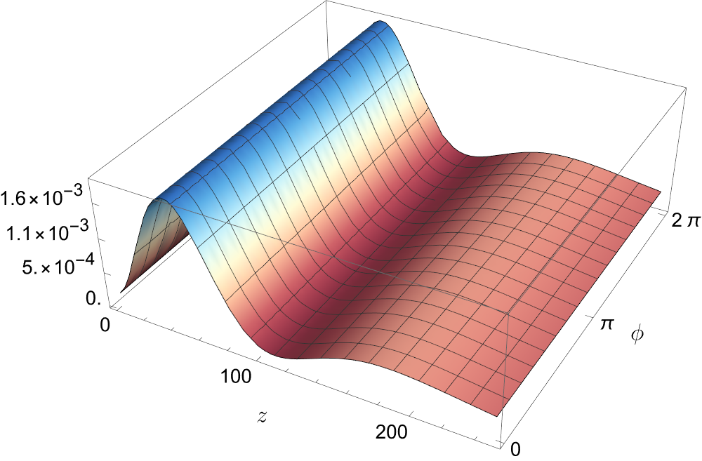
Figure 1: Normalized probability density $\mathcal{P}$ as a function of the coordinates $(\phi,\,z)$ for a nanoscroll geometry with parameters $N=4$,  $R=15$,  $D=100$,  $g=10^{-3}$,  $\alpha=1.5\times 10^{-2}$,  $v_{0}=50$,  $w_{0}=100$ .

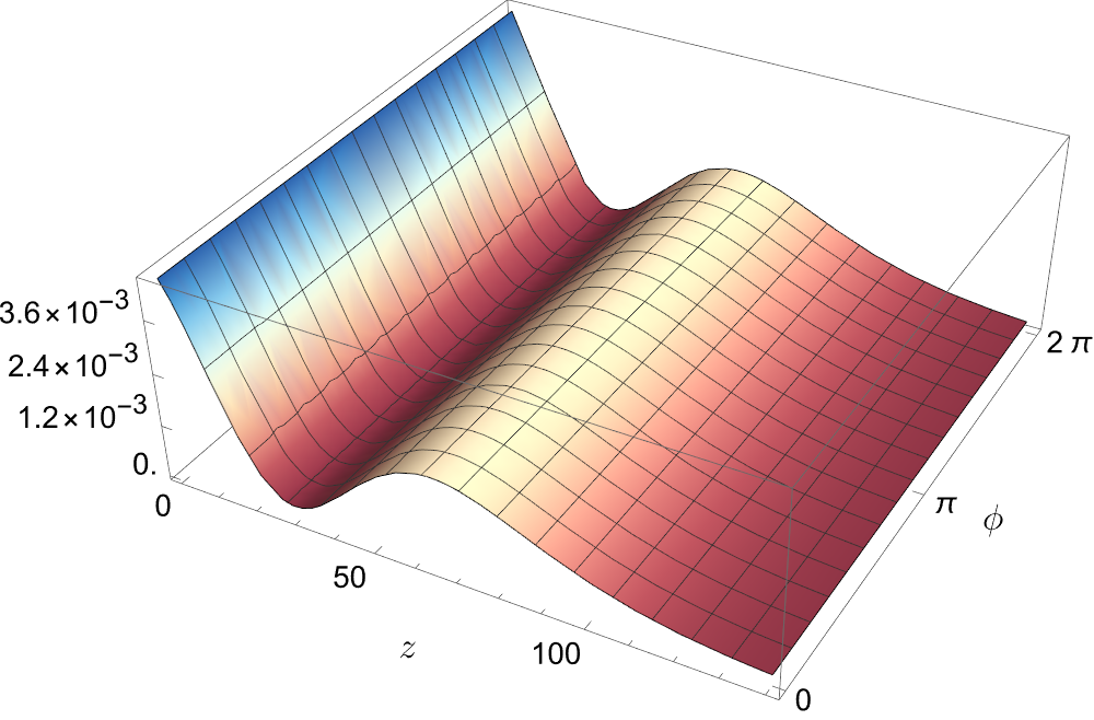
Figure 2: Normalized probability density $\mathcal{P}$ as a function of the coordinates $(\phi,\,z)$ for a nanoscroll geometry with parameters $N=5$,  $R=5$,  $D=100$,  $g=10^{-3}$,  $\alpha=2\times 10^{-2}$,  $v_{0}=200$,  $w_{0}=100$ .

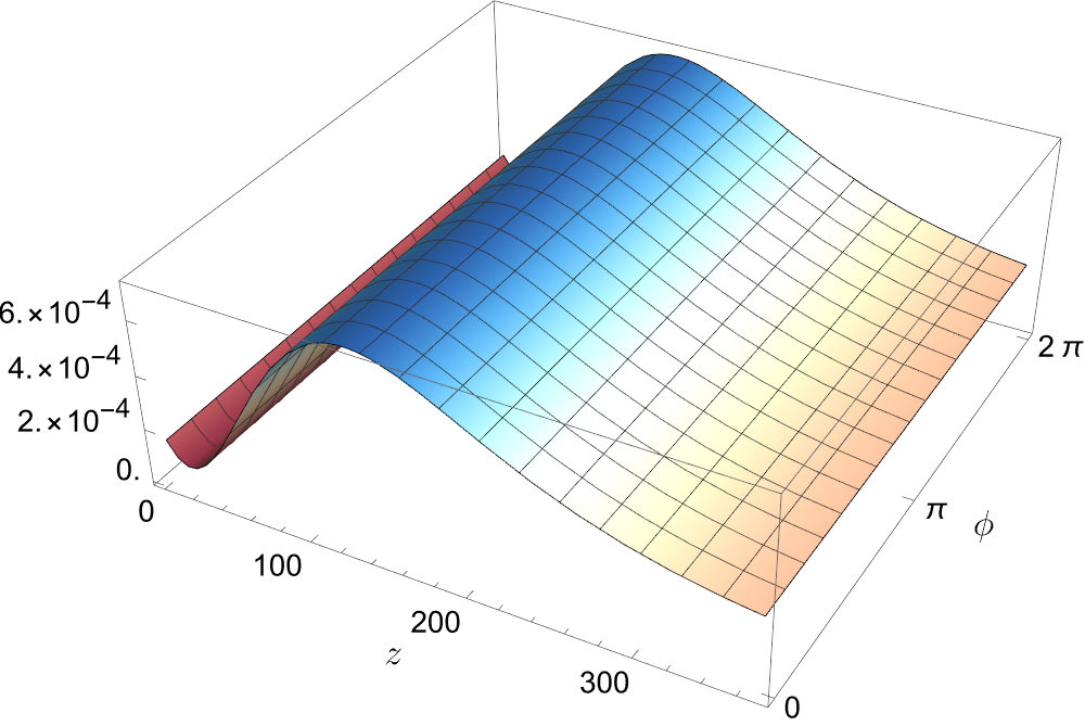
Figure 3: Normalized probability density $\mathcal{P}$ as a function of the coordinates $(\phi,\,z)$ for a nanoscroll geometry with parameters $N=3$,  $R=30$,  $D=100$,  $g=10^{-3}$,  $\alpha=10^{-2}$,  $v_{0}=90$,  $w_{0}=15$ .

We can see that the structure of the probability density function is weakly affected by displacements along the $\phi$ coordinate, while its variation is non-trivial along the $z$ direction, in agreement with our choice (28).

4.3  Local density of states

Given a location $X$ on the layer surface and an energy value $E$, the local density of states (LDOS) of the sample can be expressed in terms of the probability density as [110]

$$\rho_{{}_{\textsc{s}}}(E,X,0)=\frac{1}{\varepsilon}\>\sum_{E-\varepsilon}^{E}\mathcal{P}(X)\>,$$ (42)

for small values of $\varepsilon$, where the $0$–coordinate states that we are considering pseudoparticles on a two-dimensional space (zero-distance from the substrate surface). The LDOS then expresses the number of charge carriers per unit surface and unit energy range of size $\varepsilon$, at a given surface location $X$ and energy $E$. The sample LDOS is not only an interesting direct physical observable, but also a substrate feature of great importance for electronic applications, being the availability of empty valence and conduction states (states below and above the Fermi level) crucial for the transition rates.

Measurements.

The sample LDOS can be mapped using a scanning tunneling microscope (STM). The latter is an experimental device based on quantum mechanical tunneling, where the wave-like properties of charge carries allow them to penetrate, through a potential barrier, into regions that are forbidden to them in the classical picture. STM spectroscopy provides insight into the surface electronic properties of the substrate, being the tunneling current strongly affected by the local density of states $\rho_{{}_{\textsc{s}}}$. The latter is in turn related to the probability density $\mathcal{P}$ through definition (42).

A typical STM device consists of sharp conductive tip, brought within tunneling distance ($<\mathrm{nm}$) from a sample surface. A small voltage bias $V$ is then applied between the probe tip and the substrate, causing charge carriers to tunnel across the gap, resulting in a tunneling current between the sample and the tip.

In the STM–map setup, the density of states at some fixed energy is mapped as a function of the position $(\phi,\,z)$ on the sample surface. If we assume $\varepsilon=e\,V$ to be very small with respect to the work function $\Phi_{\textsc{w}}$ (minimum energy required to extract an electron from the surface), the sample states with energy lying between $E_{\textsc{f}}-\varepsilon$ and $E_{\textsc{f}}$ are very close to the Fermi level and have non-zero probability of tunneling into the tip. The resulting tunneling current $\mathcal{I}$ is directly proportional to the number of states on the substrate within our energy range of width $\varepsilon$, this number depending on the local properties of the surface. Including all the sample states in the chosen energy range, the measured tunneling current can be modeled, in first approximation, as [110]

$$\mathcal{I}~{}\propto\,\sum_{E_{\textsc{f}}-e\,V}^{E_{\textsc{f}}}\mathcal{P}\;e^{-2\,\Lambda\,d}\;,$$ (43)

where $\Lambda$ is some decay constant in the barrier separation depending on $\Phi_{\textsc{w}}$ . The exponential function gives the suppression for charge carriers tunneling in the classically forbidden region of width $d$ (sample-tip separation). The tunneling current can be then measured, for constant separation $d$, at different $X$ positions and, for sufficiently small $V$, it can be conveniently expressed in terms of the LDOS of the sample as [110]:

$$\mathcal{I}(X)~{}\propto~{}\,\rho_{{}_{\textsc{s}}}(E_{\textsc{f}},X,0)\;e^{-2\,\Lambda\,d}\;e\,V\;.$$ (44)

For finite bias voltage and different Fermi levels for the sample and tip, the tunneling current and its relation with the sample local density of states can be obtained from Bardeen time-dependent perturbation approach [110].

5  Summary

The study of graphene-like systems is a captivating and multidisciplinary field of research, combining notion and techniques from quantum mechanics, general relativity and condensed matter physics. These special materials realize the physics of Dirac fermions in a real laboratory framework, the substrate acting as a lower-dimensional curved spacetime for the charge carriers. This provides a direct connection between condensed matter and theoretical quantum models, with the possibility to explore the analogues of many high energy physics effects in a solid-state system [111, 112, 113, 114, 115, 116, 117, 118, 119, 120, 121, 122].

In this paper we studied the governing equations of the charge carriers in Dirac materials, in the presence of a local Fermi velocity and non-trivial energy-mass parameters. The curvature of the sample mimics a curved spacetime background for the Dirac pseudoparticles, whose dynamics is then governed by a suitably modified Dirac equation. The procedure led us to an analytic expression for the wave functions of the quasiparticle modes, which was then applied to an explicitly example involving a nanoscroll geometry. We also discussed the impact on the sample density of states as a simple and straightforward physical observable.

Acknowledgments.

BB thanks Shiv Nadar Institute of Eminence for the initial support of this work. BB also thanks Mr. Phalguni Mookhopadhayay, Chancellor Brainware University, for constant encouragement. RG thanks Shiv Nadar University for the grant of senior research fellowship. AG thanks prof. Francesco Laviano that supported these studies with his funds.

Data availability statement.

All data supporting this study are included in the article.

Conflict of interest.

The authors declare no conflict of interest.

References

- [1] B. Thaller, “The Dirac Equation”; Springer Verlag, Berlin, DE (1992).
- [2] J.D. Bjorken and S.D. Drell, “Relativistic quantum fields”; McGraw-Hill, New York, USA (1965).
- [3] M.E. Peskin and D.V. Schroeder, “An Introduction to quantum field theory”; Addison-Wesley, Reading, USA (1995).
- [4] K. Novoselov, A. Geim, S. Morozov, D. Jiang, Y. Zhang, S. Dubonos, I. Grigorieva and A. Firsov, “Electric Field Effect in Atomically Thin Carbon Films”, Science 306 (2004), n. 5696, 666–669.
- [5] K.S. Novoselov, A.K. Geim, S.V. Morozov, D. Jiang, M.I. Katsnelson, I.V. Grigorieva, S.V. Dubonos and A.A. Firsov, “Two-dimensional gas of massless Dirac fermions in graphene”, Nature 438 (2005) 197, [cond-mat/0509330].
- [6] V. Gusynin, S. Sharapov and J. Carbotte, “Unusual microwave response of Dirac quasiparticles in graphene”, Phys. Rev. Lett. 96 (2006) 256802, [cond-mat/0603267].
- [7] M. Katsnelson and K. Novoselov, “Graphene: New bridge between condensed matter physics and quantum electrodynamics”, Solid State Commun. 143 (2007), n. 1, 3–13.
- [8] A.H. Castro Neto, F. Guinea, N.M.R. Peres, K.S. Novoselov and A.K. Geim, “The electronic properties of graphene”, Rev. Mod. Phys. 81 (2009) 109–162, [arXiv:0709.1163].
- [9] A.K. Geim and K.S. Novoselov, “The rise of graphene”, Nat. Mater. 6 (2007), n. 3, 183.
- [10] A. Cortijo and M. Vozmediano, “Effects of topological defects and local curvature on the electronic properties of planar graphene”, Nucl. Phys. B 763 (2007) 293–308, [cond-mat/0612374].
- [11] A.K. Geim, “Graphene: status and prospects”, Science 324 (2009), n. 5934, 1530–1534.
- [12] M. Vozmediano, M. Katsnelson and F. Guinea, “Gauge fields in graphene”, Phys. Rept. 496 (2010) 109–148, [arXiv:1003.5179].
- [13] B. Amorim, A. Cortijo, F. De Juan, A. Grushin, F. Guinea, A. Gutiérrez-Rubio, H. Ochoa, V. Parente et al., “Novel effects of strains in graphene and other two dimensional materials”, Phys. Rept. 617 (2016) 1–54, [arXiv:1503.00747].
- [14] C. Downing and M. Portnoi, “Massless Dirac fermions in two dimensions: Confinement in nonuniform magnetic fields”, Phys. Rev. B 94 (2016), n. 16, 165407, [arXiv:1610.03032].
- [15] A. Gallerati, “Graphene properties from curved space Dirac equation”, Eur. Phys. J. Plus 134 (2019), n. 5, 202, [arXiv:1808.01187].
- [16] F. Fillion-Gourdeau, E. Lorin and S. MacLean, “Numerical quasiconformal transformations for electron dynamics on strained graphene surfaces”, Phys. Rev. E 103 (2021), n. 1, 013312.
- [17] A. Gallerati, “Negative-curvature spacetime solutions for graphene”, J. Phys. Condens. Matt. 33 (2021), n. 13, 135501, [arXiv:2101.03010].
- [18] B. Hamil and B.C. Lütfüoğlu, “Dunkl graphene in constant magnetic field”, Eur. Phys. J. Plus 137 (2022), n. 11, 1241, [arXiv:2208.11729].
- [19] M. De Oliveira, “Connecting the Dirac Equation in Flat and Curved Spacetimes via Unitary Transformation”, Few-Body Syst. 63 (2022), n. 2, 1–11.
- [20] O. Vafek and A. Vishwanath, “Dirac Fermions in Solids: From High-T cuprates and Graphene to Topological Insulators and Weyl Semimetals”, Ann. Rev. Condens. Matter Phys. 5 (2014) 83–112, [arXiv:1306.2272].
- [21] X. Li, X. Wang, L. Zhang, S. Lee and H. Dai, “Chemically derived, ultrasmooth graphene nanoribbon semiconductors”, Science 319 (2008), n. 5867, 1229–1232.
- [22] S. Stankovich, D. Dikin, G. Dommett, K. Kohlhaas, E. Zimney, E. Stach, R. Piner, S. Nguyen and R. Ruoff, “Graphene-based composite materials”, Nature 442 (2006), n. 7100, 282–286.
- [23] F. Bonaccorso, Z. Sun, T. Hasan and A. Ferrari, “Graphene photonics and optoelectronics”, Nature Phot. 4 (2010), n. 9, 611–622.
- [24] Z. Sun, T. Hasan, F. Torrisi, D. Popa, G. Privitera, F. Wang, F. Bonaccorso, D. Basko and A. Ferrari, “Graphene mode-locked ultrafast laser”, ACS Nano 4 (2010), n. 2, 803–810.
- [25] C. Lui, K. Mak, J. Shan, T. Heinz et al., “Ultrafast photoluminescence from graphene”, Phys. Rev. Lett. 105 (2010), n. 12, 127404.
- [26] E.Y. Andrei, G. Li and X. Du, “Electronic properties of graphene: a perspective from scanning tunneling microscopy and magneto-transport”, Rept. Prog. Phys. 75 (2012) 056501, [arXiv:1204.4532].
- [27] N.M.R. Peres, “Colloquium: The Transport properties of graphene: An Introduction”, Rev. Mod. Phys. 82 (2010) 2673–2700, [arXiv:1007.2849].
- [28] A. Cortijo and M. Vozmediano, “Electronic properties of curved graphene sheets”, EPL 77 (2007), n. 4, 47002, [cond-mat/0603717].
- [29] H. Kleinert, “Gauge fields in condensed matter”; World Scientific, Singapore (1989).
- [30] F. De Juan, M. Sturla and M. Vozmediano, “Space dependent Fermi velocity in strained graphene”, Phys. Rev. Lett. 108 (2012), n. 22, 227205, [arXiv:1201.2656].
- [31] Kim, K. and Lee, Z. and Malone, B.D. and Chan, K.T. and Alemán, B. and Regan, W. and Gannett, W. and Crommie, M.F. and Cohen, M.L. and Zettl, A., “Multiply folded graphene”, Phys. Rev. B 83 (2011), n. 24, 245433.
- [32] M. Fogler, A.C. Neto and F. Guinea, “Effect of external conditions on the structure of scrolled graphene edges”, Phys. Rev. B 81 (2010), n. 16, 161408.
- [33] A. Gallerati, “Graphene, Dirac equation and analogue gravity”, Phys. Scripta 97 (2022), n. 6, 064005, [arXiv:2205.08843].
- [34] F. de Juan, A. Cortijo and M.A. Vozmediano, “Charge inhomogeneities due to smooth ripples in graphene sheets”, Phys. Rev. B 76 (2007), n. 16, 165409.
- [35] G. Gui, J. Li and J. Zhong, “Band structure engineering of graphene by strain: First-principles calculations”, Phys. Rev. B 78 (2008), n. 7, 075435.
- [36] F. de Juan, J.L. Manes and M.A. Vozmediano, “Gauge fields from strain in graphene”, Phys. Rev. B 87 (2013), n. 16, 165131.
- [37] M. Oliva-Leyva and G.G. Naumis, “Generalizing the Fermi velocity of strained graphene from uniform to nonuniform strain”, Physics Letters A 379 (2015), n. 40-41, 2645–2651.
- [38] J.R. Lima and F. Moraes, “Indirect band gap in graphene from modulation of the Fermi velocity”, Solid State Communications 201 (2015) 82–87.
- [39] C. Downing and M. Portnoi, “Localization of massless Dirac particles via spatial modulations of the Fermi velocity”, J. Phys. Condens. Matt. 29 (2017), n. 31, 315301.
- [40] H. Yan, Z. Chu, W. Yan, M. Liu, L. Meng, M. Yang, Y. Fan, J. Wang, R. Dou, Y. Zhang et al., “Superlattice Dirac points and space-dependent Fermi velocity in a corrugated graphene monolayer”, Phys. Rev. B 87 (2013), n. 7, 075405.
- [41] C. Hwang, D.A. Siegel, S.K. Mo, W. Regan, A. Ismach, Y. Zhang, A. Zettl and A. Lanzara, “Fermi velocity engineering in graphene by substrate modification”, Sci. Rep. 2 (2012), n. 1, 590.
- [42] W. Jang, H. Kim, Y. Shin, M. Wang, S. Jang, M. Kim, S. Lee, S. Kim, Y. Song and S. Kahng, “Observation of spatially-varying Fermi velocity in strained-graphene directly grown on hexagonal boron nitride”, Carbon 74 (2014) 139–145.
- [43] A.L. Phan and D.N. Le, “Electronic transport in two-dimensional strained Dirac materials under multi-step Fermi velocity barrier: transfer matrix method for supersymmetric systems”, Eur. Phys. J. B 94 (2021), n. 8, 165, [arXiv:2106.10902].
- [44] M. Oliva-Leyva, J. Barrios-Vargas and C. Wang, “Fingerprints of a position-dependent Fermi velocity on scanning tunnelling spectra of strained graphene”, J. Phys. Condens. Matt. 30 (2018), n. 8, 085702.
- [45] M. Oliva-Leyva, J. Barrios-Vargas and G. De la Cruz, “Effective magnetic field induced by inhomogeneous Fermi velocity in strained honeycomb structures”, Phys. Rev. B 102 (2020), n. 3, 035447.
- [46] A. Ishkhanyan and V. Jakubský, “Two-dimensional Dirac fermion in presence of an asymmetric vector potential”, J. Phys. A 51 (2018), n. 49, 495205, [arXiv:1801.05045].
- [47] O. Mustafa, “(1+1)-Dirac bound states in one dimension, with position-dependent Fermi velocity and mass”, Open Physics 11 (2013), n. 4, 480–486.
- [48] R. Ghosh, “Position-dependent mass Dirac equation and local Fermi velocity”, J. Phys. A 55 (2022), n. 1, 015307, [arXiv:2107.01668].
- [49] B. Bagchi, R. Ghosh and C. Quesne, “so(2, 1) algebra, local Fermi velocity, and position-dependent mass Dirac equation”, J. Phys. A 55 (2022), n. 37, 375204, [arXiv:2205.02017].
- [50] R. Valencia-Torres, J. Avendaño, J. García-Ravelo and E. Choreño, “Position-dependent mass with modulated velocity in 1-D heterostructures”, Phys. Scripta 97 (2022), n. 10, 105306.
- [51] J.L. Manes, “Symmetry-based approach to electron-phonon interactions in graphene”, Phys. Rev. B 76 (2007), n. 4, 045430.
- [52] C.H. Park and S.G. Louie, “Making massless Dirac fermions from a patterned two-dimensional electron gas”, Nano Lett. 9 (2009), n. 5, 1793–1797.
- [53] N.M.R. Peres, “Scattering in one-dimensional heterostructures described by the Dirac equation”, J. Phys. Condens. Matter 21 (2009) 095501, [arXiv:0901.4857].
- [54] G. Giovannetti, P.A. Khomyakov, G. Brocks, P.J. Kelly and J. Van Den Brink, “Substrate-induced band gap in graphene on hexagonal boron nitride: Ab initio density functional calculations”, Phys. Rev. B 76 (2007), n. 7, 073103.
- [55] S.Y. Zhou, G.H. Gweon, A. Fedorov, d. First, P.N., W. De Heer, D.H. Lee, F. Guinea, A.C. Neto and A. Lanzara, “Substrate-induced bandgap opening in epitaxial graphene”, Nature materials 6 (2007), n. 10, 770.
- [56] B. Bagchi, P. Gorain, C. Quesne and R. Roychoudhury, “A general scheme for the effective-mass Schrödinger equation and the generation of the associated potentials”, Mod. Phys. Lett. A 19 (2004), n. 37, 2765–2775.
- [57] B. Bagchi, A. Banerjee, C. Quesne and V. Tkachuk, “Deformed shape invariance and exactly solvable Hamiltonians with position-dependent effective mass”, J. Phys. A Math. Theor. 38 (2005), n. 13, 2929.
- [58] N. Peres, A. Neto and F. Guinea, “Dirac fermion confinement in graphene”, Phys. Rev. B 73 (2006), n. 24, 241403.
- [59] R. Grassi, S. Poli, E. Gnani, A. Gnudi, S. Reggiani and G. Baccarani, “Tight-binding and effective mass modeling of armchair graphene nanoribbon FETs”, Solid State Electron. 53 (2009), n. 4, 462–467.
- [60] C. Yannouleas, I. Romanovsky and U. Landman, “Beyond the constant-mass Dirac physics: Solitons, charge fractionization, and the emergence of topological insulators in graphene rings”, Phys. Rev. B 89 (2014), n. 3, 035432.
- [61] K. Reijnders, D. Minenkov, M. Katsnelson and S. Dobrokhotov, “Electronic optics in graphene in the semiclassical approximation”, Ann. Phys. 397 (2018) 65–135.
- [62] R.R.S. Oliveira, A.A. Araújo Filho, R.V. Maluf and C.A.S. Almeida, “The relativistic Aharonov–Bohm–Coulomb system with position-dependent mass”, J. Phys. A 53 (2020), n. 4, 045304, [arXiv:1812.07756].
- [63] A. Contreras-Astorga, D.J. Fernández C and J. Negro, “Solutions of the Dirac equation in a magnetic field and intertwining operators”, Symm. Integr. Geom. 8 (2012) 082.
- [64] C. Downing and M. Portnoi, “Trapping charge carriers in low-dimensional Dirac materials”, Int. J. Nanosci. 18 (2019), n. 03n04, 1940001.
- [65] F. Serafim, F. Santos, J. Lima, C. Filgueiras and F. Moraes, “Position-dependent mass effects in the electronic transport of two-dimensional quantum systems: Applications to nanotubes”, Physica E 108 (2019) 139–146.
- [66] A. Schulze-Halberg, “Arbitrary-order Darboux transformations for two-dimensional Dirac equations with position-dependent mass”, Eur. Phys. J. Plus 135 (2020), n. 3, 1–13.
- [67] A. Schulze-Halberg, “Higher-order Darboux transformations for the Dirac equation with position-dependent mass at nonvanishing energy”, Eur. Phys. J. Plus 135 (2020), n. 10, 863.
- [68] A. Schulze-Halberg, “Darboux transformations for Dirac equations in polar coordinates with vector potential and position-dependent mass”, Eur. Phys. J. Plus 137 (2022), n. 7, 1–16.
- [69] C. Tezcan, R. Sever and O. Yesiltas, “A new approach to the exact solutions of the effective mass Schrodinger equation”, Int. J. Theor. Phys. 47 (2008) 1713.
- [70] S. Raghu and F. Haldane, “Analogs of quantum-Hall-effect edge states in photonic crystals”, Phys. Rev. A 78 (2008), n. 3, 033834.
- [71] B. Bernevig and T. Hughes, “Topological Insulators and Topological Superconductors”; Princeton University Press, Princeton, USA (2013).
- [72] P. Xie and Y. Zhu, “Wave packet dynamics in slowly modulated photonic graphene”, J. Differ. Equ. 267 (2019), n. 10, 5775–5808.
- [73] P. Hu, L. Hong and Y. Zhu, “Linear and nonlinear electromagnetic waves in modulated honeycomb media”, Stud. Appl. Math. 144 (2020), n. 1, 18–45.
- [74] O. von Roos, “Position-dependent effective masses in semiconductor theory”, Phys. Rev. B 27 (1983) 7547–7552.
- [75] Zhang, D.B. and Akatyeva, E. and Dumitrică, T., “Bending ultrathin graphene at the margins of continuum mechanics”, Phys. Rev. Lett. 106 (2011), n. 25, 255503.
- [76] Z. Xu and M.J. Buehler, “Geometry controls conformation of graphene sheets: membranes, ribbons, and scrolls”, ACS Nano 4 (2010), n. 7, 3869–3876.
- [77] P. Castro-Villarreal and R. Ruiz-Sánchez, “Pseudomagnetic field in curved graphene”, Phys. Rev. B 95 (2017), n. 12, 125432, [arXiv:1612.04305].
- [78] P.A. Morales and P. Copinger, “Curvature-induced pseudogauge fields from time-dependent geometries in graphene”, Phys. Rev. B 107 (2023), n. 7, 075432, [arXiv:2209.03378].
- [79] V. Fock, “Geometrization of the Dirac theory of electrons”, Zeitschrift für Physik 57 (1929), n. 3-4, 261–277.
- [80] L. Parker and D. Toms, “Quantum field theory in curved spacetime: quantized fields and gravity”; Cambridge University Press, Cambridge, UK (2009).
- [81] G.H. Liang, Y.L. Wang, M.Y. Lai, H. Liu, H.S. Zong and S.N. Zhu, “Pseudo-magnetic-field and effective spin-orbit interaction for a spin-1/2 particle confined to a curved surface”, Phys. Rev. A 98 (2018), n. 6, 062112.
- [82] Y.L. Wang, M.Y. Lai, F. Wang, H.S. Zong and Y.F. Chen, “Geometric effects resulting from square and circular confinements for a particle constrained to a space curve”, Phys. Rev. A 97 (2018), n. 4, 042108.
- [83] A. Concha and Z. Tešanović, “Effect of a velocity barrier on the ballistic transport of Dirac fermions”, Phys. Rev. B 82 (2010), n. 3, 033413.
- [84] O. Panella and P. Roy, “Bound state in continuum-like solutions in one-dimensional heterostructures”, Phys. Lett. A 376 (2012), n. 38-39, 2580–2583.
- [85] A. Raoux, M. Polini, R. Asgari, A. Hamilton, R. Fazio and A.H. MacDonald, “Velocity-modulation control of electron-wave propagation in graphene”, Phys. Rev. B 81 (2010), n. 7, 073407.
- [86] P. Krstajić and P. Vasilopoulos, “Ballistic transport through graphene nanostructures of velocity and potential barriers”, J. Phys. Condens. Matt. 23 (2011), n. 13, 135302.
- [87] G. Bastard, “Wave mechanics applied to semiconductor heterostructures”; John Wiley and Sons Inc., New York, USA (1990).
- [88] S. de-la Huerta-Sainz, A. Ballesteros and N.A. Cordero, “Gaussian Curvature Effects on Graphene Quantum Dots”, Nanomaterials 13 (2022), n. 1, 95.
- [89] P. Ring and P. Schuck, “The nuclear many-body problem”; Springer-Verlag, Berlin, DE (2004).
- [90] B. Bagchi and T. Tanaka, “A generalized non-Hermitian oscillator Hamiltonian, N-fold supersymmetry and position-dependent mass models”, Phys. Lett. A 372 (2008), n. 33, 5390–5393.
- [91] C. Quesne, “Infinite families of position-dependent mass Schrödinger equations with known ground and first excited states”, Annals Phys. 399 (2018) 270–288, [arXiv:1808.07367].
- [92] S. Cruz y Cruz and O. Rosas-Ortiz, “Position-dependent mass oscillators and coherent states”, J. Phys. A Math. Theor. 42 (2009), n. 18, 185205.
- [93] M. Znojil and G. Levai, “Schrödinger equations with indefinite effective mass”, Phys. Lett. A 376 (2012), n. 45, 3000–3005.
- [94] C. Quesne, “Point canonical transformation versus deformed shape invariance for position-dependent mass Schrödinger equations”, Symm. Integr. Geom. 5 (2009) 046.
- [95] F. de Juan, A. Cortijo and M. Vozmediano, “Charge inhomogeneities due to smooth ripples in graphene sheets”, Phys. Rev. B 76 (2007), n. 16, 165409.
- [96] M.A. dos Santos, I.S. Gomez, B.G. da Costa and O. Mustafa, “Probability density correlation for PDM-Hamiltonians and superstatistical PDM-partition functions”, Eur. Phys. J. Plus 136 (2021), n. 1, 96.
- [97] S.H. Dong, W.H. Huang, P. Sedaghatnia and H. Hassanabadi, “Exact solutions of an exponential type position dependent mass problem”, Results in Physics 34 (2022) 105294.
- [98] B. Gönül, O. Özer, B. GönüL and F. Üzgün, “Exact solutions of effective-mass Schrödinger equations”, Mod. Phys. Lett. A 17 (2002), n. 37, 2453–2465.
- [99] R. Valencia-Torres, J. Avendaño, J. García-Ravelo and E. Choreño, “Position-dependent mass with modulated velocity in 1-D heterostructures”, Phys. Scripta 97 (2022), n. 10, 105306.
- [100] X. Xie, L. Ju, X. Feng, Y. Sun, R. Zhou, K. Liu, S. Fan, Q. Li and K. Jiang, “Controlled fabrication of high-quality carbon nanoscrolls from monolayer graphene”, Nano Lett. 9 (2009), n. 7, 2565–2570.
- [101] Braga, S.F. and Coluci, V.R. and Legoas, S.B. and Giro, R. and Galvão, D.S. and Baughman, R.H., “Structure and dynamics of carbon nanoscrolls”, Nano Lett. 4 (2004), n. 5, 881–884.
- [102] Y. Chen, J. Lu and Z. Gao, “Structural and electronic study of nanoscrolls rolled up by a single graphene sheet”, J. Phys. Chem. C 111 (2007), n. 4, 1625–1630.
- [103] G. Mpourmpakis, E. Tylianakis and G. Froudakis, “Carbon nanoscrolls: a promising material for hydrogen storage”, Nano Lett. 7 (2007), n. 7, 1893–1897.
- [104] D. Berman, S. Deshmukh, S. Sankaranarayanan, A. Erdemir and A. Sumant, “Macroscale superlubricity enabled by graphene nanoscroll formation”, Science 348 (2015), n. 6239, 1118–1122.
- [105] H. Li, R. Papadakis, S. Jafri, T. Thersleff, J. Michler, H. Ottosson and K. Leifer, “Superior adhesion of graphene nanoscrolls”, Commun. Phys. 1 (2018), n. 1, 1–7.
- [106] S. Saini, S. Reshmi, G. Gouda, A. Kumar, K. Sriram and K. Bhattacharjee, “Low reflectance of carbon nanotube and nanoscroll-based thin film coatings: a case study”, Nanoscale Advances 3 (2021), n. 11, 3184–3198.
- [107] X. Chen, Q. Zhou, J. Wang and Q. Chen, “Formation of Graphene Nanoscrolls and Their Electronic Structures Based on Ab Initio Calculations”, J. Phys. Chem. Lett 13 (2022) 2500–2506.
- [108] M. Trushin and A. Neto, “Stability of a rolled-up conformation state for two-dimensional materials in aqueous solutions”, Phys. Rev. Lett. 127 (2021), n. 15, 156101.
- [109] M. Hassanzadazar, M. Ahmadi, R. Ismail and H. Goudarzi, “Electrical property analytical prediction on Archimedes chiral carbon nanoscrolls”, J. Electron. Mater. 45 (2016), n. 10, 5404–5411.
- [110] C.J. Chen, “Introduction to scanning tunneling microscopy”; Oxford University Press, 1 ed. (1993).
- [111] M. Cvetic and G. Gibbons, “Graphene and the Zermelo Optical Metric of the BTZ Black Hole”, Annals Phys. 327 (2012) 2617–2626, [arXiv:1202.2938].
- [112] T. Stegmann and N. Szpak, “Current flow paths in deformed graphene: from quantum transport to classical trajectories in curved space”, New J. Phys. 18 (2016), n. 5, 053016, [arXiv:1512.06750].
- [113] P.D. Alvarez, M. Valenzuela and J. Zanelli, “Supersymmetry of a different kind”, JHEP 04 (2012) 058, [arXiv:1109.3944].
- [114] A. Sepehri, R. Pincak and A.F. Ali, “Emergence of F(R) gravity-analogue due to defects in graphene”, Eur. Phys. J. B 89 (2016), n. 11, 250, [arXiv:1606.02039].
- [115] M. Franz and M. Rozali, “Mimicking black hole event horizons in atomic and solid-state systems”, Nature Rev. Mater. 3 (2018) 491–501, [arXiv:1808.00541].
- [116] S. Capozziello, R. Pincak and E.N. Saridakis, “Constructing superconductors by graphene Chern-Simons wormholes”, Annals Phys. 390 (2018) 303–333.
- [117] J.S. Pedernales, M. Beau, S.M. Pittman, I.L. Egusquiza, L. Lamata, E. Solano and A. del Campo, “Dirac Equation in (1+1)-Dimensional Curved Spacetime and the Multiphoton Quantum Rabi Model”, Phys. Rev. Lett. 120 (2018), n. 16, 160403, [arXiv:1707.07520].
- [118] B. Kandemir, “Hairy BTZ black hole and its analogue model in graphene”, Annals Phys. 413 (2020) 168064, [arXiv:1907.03509].
- [119] L. Andrianopoli, B.L. Cerchiai, R. D’Auria, A. Gallerati, R. Noris, M. Trigiante and J. Zanelli, “-extended supergravity, unconventional SUSY and graphene”, JHEP 01 (2020) 084, [arXiv:1910.03508].
- [120] A. Gallerati, “Supersymmetric theories and graphene”, PoS 390 (2021) 662, [arXiv:2104.07420].
- [121] T. Morresi, D. Binosi, S. Simonucci, R. Piergallini, S. Roche, N. Pugno and T. Simone, “Exploring event horizons and Hawking radiation through deformed graphene membranes”, 2D Materials 7 (2020), n. 4, 041006.
- [122] S. Capozziello, R. Pinčak and E. Bartoš, “Chern-Simons Current of Left and Right Chiral Superspace in Graphene Wormhole”, Symmetry 12 (2020), n. 5, 774.