Convergence of Allen–Cahn equations to De Giorgi’s multiphase mean curvature flow

Abstract

This paper presents a conditional convergence result of solutions to the Allen–Cahn equation with arbitrary potentials to a De Giorgi type $\operatorname{BV}$-solution to multiphase mean curvature flow. Moreover we show that De Giorgi type $\operatorname{BV}$-solutions are De Giorgi type varifold solutions, and thus our solution is unique in a weak-strong sense.
Keywords: Gradient flows, Mean curvature flow, Allen–Cahn equation
Mathematical Subject Classification: 35A15, 35K57, 35K93, 53E10, 74N20

1 Introduction

1.1 History and main results

Multiphase mean curvature flow is an important geometric evolution equation which has been studied for a long time, bearing not only mathematical importance, but also for the applied sciences. Originally it was proposed to study the evolution of grain boundaries in annealed recrystallized metal, as described by Mullins in [Mul56], who cites Beck in [Bec52] as already having observed such a behaviour in 1952.

Over the years numerous different solution concepts for multiphase mean curvature flow have been proposed. Classically we have smooth solutions, where we require the evolution of the interfaces to be smooth, for example described by Huisken in [Hui90]. Another description of smoothly evolving mean curvature flow can be found in the work of Gage and Hamilton [GH86], who proved the “shrinking conjecture” for convex planar curves. Brakke describes in his book [Bra78] the motion by mean curvature using varifolds, which yields a quite abstract and general notion for mean curvature flow and is based on the gradient flow structure of mean curvature flow. Luckhaus and Sturzenhecker introduced a distributional solution concept for mean curvature flow in their work [LS95]. Another approach is the viscosity solution concept presented in [CGG91] and [ES91], where it is shown that solutions of a certain parabolic equation have the property that if they are smooth, the corresponding level sets move by mean curvature.

For some smooth potential $W\colon\mathbb{R}^{N}\to[0,\infty)$ with finitely many zeros $\alpha_{1},\dotsc,\alpha_{P}$, the Allen–Cahn equation

$$\partial_{t}u_{\varepsilon}=\Delta u_{\varepsilon}-\frac{1}{\varepsilon^{2}}\nabla W(u_{\varepsilon})$$ (1)

is commonly used as a phase-field approximation for mean curvature flow and was first proposed by Allen and Cahn in their paper [AC79]. Since then it has been an extensively researched topic, both from a numerical and analytical standpoint.

If we consider the two-phase case, which corresponds to setting $N=1$ and $P=2$, then the behaviour of the solutions to (1) as $\varepsilon$ tends to zero are thoroughly researched. The authors Bronsard and Kohn showed in [BK91] the compactness of solutions and regularity for the limit by exploiting the gradient flow structure of (1), more precisely by mainly utilizing the corresponding energy dissipation inequality. Moreover they studied the behaviour for radially symmetric initial data and showed that the limit moves by mean curvature in this case. Chen has proven in [Che92] that as long as the interface of the limit evolves smoothly, we have convergence to (classical) mean curvature flow. A similar result has been shown by De Mottoni and Schatzmann in [DS95], where they showed short time convergence. Their strategy was to prove through a spectral estimate that the solution $u_{\varepsilon}$ already coincides with the formal asymptotic expansion up to an error. Similar strategies, but for nonlinear Robin boundary conditions with angle close to 90 degrees, can be found in the paper [AM22] by Abels and Moser.

Ilmanen made fundamental contributions in [Ilm93] by proving the convergence to Brakke’s mean curvature flow as long as the initial conditions are well-prepared by exploiting the equipartition of energies. However his methods seem to only work in the two-phase case since he uses a comparison principle whose generalization to the vectorial case is not clear.

The multiphase case for both the convergence of the Allen–Cahn equation and mean curvature flow is much more involved and a topic of current research. For the convergence of the Allen–Cahn equation, asymptotic expansions with Neumann boundary conditions have been studied by Keller, Rubinstein and Sternberg in [RSK89]. Even though they considered the vector-valued Allen–Cahn equation with a multiwell potential, their analysis restricts to the parts of the interfaces where no triple junctions appear. Bronsard and Reitich however considered in [BR93] a formal asymptotic expansion which also takes triple junctions into account for the three-phase case. Moreover they proved short-time existence for the three-phase boundary problem.

The analysis of multiphase mean curvature flow has been studied for example by Mantegazza, Novaga and Tortorelli in [MNT04], where they considered the planar case when only a single triple junction appears, and their work has been extended to several triple junctions in [Man+16]. Ilmanen, Neves and Schulze furthermore proved in [INS19] that even for non-regular initial data in the sense that Herring’s angle condition is not satisfied, we have short time existence by approximation through regular networks. For long time existence, it has been shown by Kim and Tonegawa in [KT17] through a modification of Brakke’s approximation scheme that one can obtain non-trivial mean curvature flow even with singular initial data. Recently Stuvard and Tonegawa improved this result in [ST22], where they extended their findings to more general initial data and also showed that their constructed Brakke flow is a $\operatorname{BV}$-solution to mean curvature flow.

The first main goal of this paper Theorem 4.5 is to prove a conditional convergence result of solutions to the vectorial Allen–Cahn equation (1) to a De Giorgi type $\operatorname{BV}$-solution of multiphase mean curvature flow in the sense of Definition 4.1. The proof is based mainly on a duality argument and the results of Laux and Simon in [LS18]. However the strong assumption we make here is that the Cahn–Hilliard energies of the solutions to the Allen-Cahn equation (1) converge to the perimeter functional (9) applied to the limit. This prevents that as $\varepsilon$ tends to zero, the approximate interfaces collapse, which corresponds to a loss of energy in the limit $\varepsilon\to 0$, see also the discussion in Section 4.4. In general we are inclined to believe that this assumption could fail. For example it has been shown by Bronsard and Stoth in [BS96] that for the volume preserving Allen–Cahn equation and for radial-symmetric initial data, we can have any number of higher multiplicity transition layers which are at most $C\varepsilon^{\alpha}$ apart, at least for times of order one. Here $\alpha$ is some exponent between zero and one third. However it has been proven that in some cases, the energy convergence automatically holds for suitable initial data. For example Nguyen and Wang proved in [NW20] that for mean convex initial data, we obtain the desired convergence of energies. In the context of the Almgren-Taylor-Wang scheme for mean curvature flow, this has also been done by De Philippis and Laux in [DL20].

The energy convergence assumption provides us with the important equipartition of energies, whose proof under milder assumption was the main obstacle of Ilmanen in [Ilm93]. Moreover it is the key for our localization estimates and lets us localize on the different phases of the limit. Lastly it assures that the differential $\nabla u_{\varepsilon}$ can locally up to an error be written as a rank-one matrix. In fact it is the tensor of the approximate frozen unit normal and the gradient of the geodesic distance function associated to the majority phase evaluated at $u_{\varepsilon}$, see the proof of [LS18, Prop. 3.1].

The second main goal is to compare De Giorgi type $\operatorname{BV}$-solutions to De Giorgi type varifold solutions. The latter were proposed by Hensel and Laux in [HL21]. We will show that the De Giorgi type $\operatorname{BV}$-solution concept is stronger in the sense that every $\operatorname{BV}$-solution is also a varifold solution. Since Hensel and Laux have shown weak-strong uniqueness for their varifold solution concept, it follows that we also obtain weak-strong uniqueness for our De Giorgi type $\operatorname{BV}$-solution concept, which is the best we can expect. In fact it has been shown on a numerical basis by Angenent, Chopp and Ilmanen in [AIC95] that even in three dimensions, there exists a smooth hypersurface whose evolution by mean curvature flow admits a singularity at a certain time after which we have nonuniqueness. A rigorous analysis of this phenomenon has been done in dimensions 4, 5, 6, 7 and 8 by Angenent, Ilmanen and Velázquez in [AIV02].

Let us also mention some of the closely related unanswered questions. For one Hensel and Laux have shown in [HL21] that in the two-phase case and under well prepared initial conditions, the solutions of the Allen–Cahn equation (1) converge to a De Giorgi type varifold solution. However their methods have no obvious generalization to the multiphase case without the energy convergence assumption, and one even struggles to find an approximate sequence which constructs the desired varifolds. And even then one would have to find suitable substitutions for localization which will be crucial for our proof. These localization estimates are based on De Giorgi’s structure theorem and thus only work for $\operatorname{BV}$-functions.

Another possible question would be how to generalize the results to the case of arbitrary mobilities: Throughout the paper, and also the main background papers [LS18], [HL21], it is always assumed that the mobilities are fixed through the relation $\mu_{ij}=1/\sigma_{ij}$. Here $\sigma_{ij}$ denotes the surface tension of the $(i,j)$-th interface and $\mu_{ij}$ its mobility. As proposed by Bretin, Danescu, Penuelas and Masnou in [Bre+18], passing to arbitrary mobilities should amount to multiplying an appropriate “mobility matrix” $M$ onto the right-hand side of (1) and changing the metric of the underlying space accordingly to $\langle u,v\rangle=\int\left\langle Mu\,,\,v\right\rangle\differential{x}$. The difference in their approach is to first uncouple their system so that they arrive at the scalar Allen–Cahn equation and then couple the components through a Lagrange-multiplier, which assures that the limit is a partition.

1.2 Structure of the paper

In Section 2 we first describe the concept of gradient flows in an easy setting. Moreover we derive De Giorgi’s optimal energy dissipation inequality in a simple example and discuss its usefulness for reformulating the gradient flow equation. Further we apply our observations to (multiphase) mean curvature flow.

Continuing with Section 3, we take a look at the Allen–Cahn equation and the convergence of its solutions as $\varepsilon$ tends to zero to an evolving partition by citing the results of [LS18].

Lastly in Section 4 we present new results building on the previous insights. We start off by presenting a De Giorgi type $\operatorname{BV}$-solution concept for multiphase mean curvature flow. This is followed by proving a similar conditional convergence result as in the previous section. In the final Section 4.4, we discuss the assumption of energy convergence. Moreover we show that every De Giorgi type $\operatorname{BV}$-solution is a De Giorgi type varifold solution in the sense of Hensel and Laux in [HL21], whose solution concept does not rely on the assumption of energy convergence.

1.3 Notation

• Let $u\colon\mathbb{R}^{d}\to\mathbb{R}^{N}$ be differentiable at a point $x\in\mathbb{R}^{d}$. We write $\mathrm{D}u(x)$ for the (total) derivative at $x$, which means that $\mathrm{D}u(x)\in\mathbb{R}^{N\times d}$ and $\left(\mathrm{D}u(x)\right)_{ij}=\partial_{x_{j}}u^{i}(x)$. We always use the notation $\nabla u(x)$ for the transpose of the total derivative.

• If $u\colon(0,T)\times\mathbb{R}^{d}\to\mathbb{R}^{N}$, then we denote by $\mathrm{D}u(t,x)$ respectively $\nabla u(t,x)$ only the derivatives in space, and we always write $\partial_{t}u$ for the derivative in time.

• We use the symbol $\lesssim$ if an inequality holds up to a positive constant on the right hand side. This constant must only depend on the dimensions, the chosen potential $W$ and possibly the given initial data.

• The bracket $\left\langle\>\cdot\>\,,\,\>\cdot\>\right\rangle$ is used as the Euclidean inner product. Depending on the situation, it acts on vectors or matrices. If we apply $\absolutevalue{\>\cdot\>}$ to a vector or matrix, then we always uses the norm induced by the Euclidean inner product.

• We denote by $\operatorname{C}_{\mathrm{c}}$ the compactly supported continuous functions. Note that for the flat torus $\operatorname{\mathbb{T}}$, we have $\operatorname{C}_{\mathrm{c}}(\operatorname{\mathbb{T}})=\operatorname{C}(\operatorname{\mathbb{T}})$.

• For a locally integrable function $u\colon(0,T)\times\Omega\to\mathbb{R}$ with $\Omega\subseteq\mathbb{R}^{d}$ being some open set or the flat torus, we denote the total variation in space for a time $t\in(0,T)$ by

  $$\absolutevalue{\nabla u(t,\cdot)}\coloneqq\sup\left\{\int_{\Omega}u(t,x)\operatorname{div}\xi(x)\differential{x}\,\colon\,\xi\in\operatorname{C}_{\mathrm{c}}^{1}(\Omega;\mathbb{R}^{d}),\absolutevalue{\xi}\leq 1\right\}$$

  and the total variation in space taken both over time and space by

  $$\absolutevalue{\nabla u}_{d+1}$$

  $$\coloneqq{} \left\{\int_{(0,T)\times\Omega}u(t,x)\operatorname{div}_{x}\xi(t,x)\differential{(t,x)}\,\colon\,\xi\in\operatorname{C}_{\mathrm{c}}^{1}((0,T)\times\Omega;\mathbb{R}^{d}),\absolutevalue{\xi}\leq 1\right\}.$$

• If $u\colon(0,T)\times\Omega\to\mathbb{R}^{N}$ is some map, then for a given time $t\in(0,T)$, we sometimes write $u(t)$ for the map $u(t)(x)\coloneqq u(t,x)$ by a slight abuse of notation.

• To shorten notation, we always write $\int\differential{x}=\int_{\operatorname{\mathbb{T}}}\differential{x}$, where $\operatorname{\mathbb{T}}$ is the flat torus.

2 Gradient flows and mean curvature flow

2.1 Gradient flows

In the simplest case, a gradient flow of a given energy $\operatorname{E}\colon\mathbb{R}^{N}\to\mathbb{R}$ with respect to the Euclidean inner product is a solution to the ordinary differential equation

$$\derivative{t}x(t)=-\nabla\operatorname{E}(x(t)),$$ (2)

where we usually prescribe some initial value $x(0)=x_{0}\in\mathbb{R}^{N}$. The central structure here is that on the right hand side of the equation, we do not have an arbitrary vector field, but the gradient of some continuously differentiable function. Remember that the gradient of a function always depends on the chosen metric of our space. In fact, the gradient $\nabla\operatorname{E}(x)$ is always the unique element of the tangent space at $x$ which satisfies

$$\left\langle\nabla\operatorname{E}(x)\,,\,y\right\rangle=\differential_{x}\operatorname{E}(y)$$

for all elements $y$ in the tangent space at $x$. In this simple setting, the tangent space at any point is exactly $\mathbb{R}^{N}$.

A solution $x$ moves in the direction of the steepest descent of the energy $\operatorname{E}$. Moreover this allows for the following computation given a continuously differentiable solution $x$ of (2):

$$\derivative{t}\operatorname{E}(x(t)) =\left\langle\nabla\operatorname{E}(x(t))\,,\,x^{\prime}(t)\right\rangle=-\absolutevalue{\nabla\operatorname{E}(x(t))}^{2}=-\absolutevalue{x^{\prime}(t)}^{2}$$

$$=-\frac{1}{2}\left(\absolutevalue{x^{\prime}(t)}^{2}+\absolutevalue{\nabla\operatorname{E}(x(t))}^{2}\right).$$

We especially obtain that the function $\operatorname{E}(x(t))$ is non-increasing, which coincides with our intuition of the steepest descent. But more precisely, we obtain from the fundamental theorem of calculus the energy dissipation identity

$$\operatorname{E}(x(T))+\frac{1}{2}\int_{0}^{T}\absolutevalue{x^{\prime}(t)}^{2}+\absolutevalue{\nabla\operatorname{E}(x(t))}^{2}\differential{t}=\operatorname{E}(x(0)).$$ (3)

One could now raise the question if this identity already characterizes equation (2). But as it turns out, we can go even one step further. Namely we only ask for De Giorgi’s optimal energy dissipation inequality given by

$$\operatorname{E}(x(T))+\frac{1}{2}\int_{0}^{T}\absolutevalue{x^{\prime}(t)}^{2}+\absolutevalue{\nabla\operatorname{E}(x(t))}^{2}\differential{t}\leq\operatorname{E}(x(0)).$$ (4)

We call this inequality optimal since as demonstrated before, we usually expect an equality to hold if $x$ is a solution to (2). Now let us assume that $x$ satisfies inequality (4) and is sufficiently regular. Then we can estimate again by the fundamental theorem of calculus that

$$\frac{1}{2}\int_{0}^{T}\absolutevalue{\nabla\operatorname{E}(x(t))+x^{\prime}(t)}^{2}\differential{t}$$

$$={} \int_{0}^{T}\left\langle\nabla\operatorname{E}(x(t))\,,\,x^{\prime}(t)\right\rangle\differential{t}+\frac{1}{2}\int_{0}^{T}\absolutevalue{x^{\prime}(t)}^{2}+\absolutevalue{\nabla\operatorname{E}(x(t))}^{2}\differential{t}$$

$$={} \operatorname{E}(x(T))-\operatorname{E}(x(0))+\frac{1}{2}\int_{0}^{T}\absolutevalue{x^{\prime}(t)}^{2}+\absolutevalue{\nabla\operatorname{E}(x(t))}^{2}\differential{t}$$

$$\leq{} 0.$$

Since we started with an integral over a non-negative function, this implies that for almost every time $t$, we have that $x^{\prime}(t)=-\nabla\operatorname{E}(x(t))$. But if $x$ and $E$ are sufficiently regular, this already implies that $x^{\prime}(t)=-\nabla\operatorname{E}(x(t))$ holds for all times $t$. Thus $x$ is a gradient flow of the energy $\operatorname{E}$.

The real strength of formulating the differential equation (2) via inequality (4) becomes clear if we want to consider gradient flows in a more complicated setting. In order to formulate equation (2), we need to have a notion of differentiation and a gradient in the target of $x$. Therefore we may use pre-Hilbert spaces or smooth Riemannian manifolds as suitable substitutes for $\mathbb{R}^{N}$.

Examples for such more complicated gradient flows include the heat equation, which can be written as the $\operatorname{L}^{2}$-gradient flow of the Dirichlet energy. Further examples include the Fokker-Planck equation, the Allen–Cahn equation and mean curvature flow. The two latter of course play a key role for us.

The observations in this section have been around for a long time and are credited to De Giorgi and his paper [De ̵93]. Sandier and Serfaty have also written an excellent paper [SS04] on this topic, as well as the book [AGS05] by Ambrosio, Gigli and Savaré, to which we refer the interested reader.

2.2 Mean curvature flow

Mean curvature flow describes the geometric evolution of a set $(\Omega(t))_{t\geq 0}$ respectively the evolution of its boundary $\Sigma(t)\coloneqq\partial\Omega(t)$. It is formulated through the equation

$$\frac{1}{\mu}V=-\sigma H\quad\text{on }\Sigma.$$ (5)

Here $\mu>0$ is a positive constant which is called the mobility and $\sigma>0$ is a positive constant as well which we define as the surface tension. By $V$ we denote the normal velocity of the set and by $H$ its mean curvature, which is defined as the sum of the principle curvatures at a given point. There are a lot of different notions of solutions to this equation as already mentioned in the introduction. For us the central structure of this equation is its gradient flow structure. Formally we want to consider the space

$$\mathcal{M}\coloneqq\left\{\text{hypersurfaces in}\operatorname{\mathbb{T}}\right\},$$

where the tangent space at a given $\Sigma\in\mathcal{M}$ consists of the normal velocities on $\Sigma$. The metric tensor at a surface $\Sigma$ of two normal velocities is then given by the rescaled $\operatorname{L}^{2}$-inner product on $\Sigma$

$$\left\langle V\,,\,W\right\rangle_{\Sigma}\coloneqq\frac{1}{\mu}\int_{\Sigma}VW\differential{\operatorname{\mathcal{H}}^{d-1}}$$ (6)

and our energy will simply be the rescaled perimeter functional

$$\operatorname{E}(\Sigma)\coloneqq\sigma\operatorname{\mathcal{H}}^{d-1}(\Sigma).$$

By [Mag12, Thm. 17.5] the first inner variation of the perimeter functional is given by the mean curvature vector. Remember moreover that by the definition of the metric (6) the gradient of the energy at a given hypersurface $\Sigma$ has to satisfy

$$\frac{1}{\mu}\int_{\Sigma}\left\langle\nabla_{\Sigma}\operatorname{E}\,,\,V\right\rangle\differential{\operatorname{\mathcal{H}}^{d-1}}=\differential_{\Sigma}\operatorname{E}(V)$$

for all normal vector fields $V$ on $\Sigma$. Combining these arguments the gradient of the energy should simply be the mean curvature vector multiplied by $\sigma\mu$. Thus the mean curvature flow equation (5) corresponds exactly to the gradient flow equation (2). Note however that this metric tensor induces a degenerate metric in the sense that the distance between any two hypersurfaces is zero, which has been shown by Michor and Mumford in [MM06].

In Section 2.1 we highlighted the importance of De Giorgi’s optimal energy dissipation inequality (4). In our setting this translates to the inequality

$$\operatorname{E}(\Sigma(T))+\frac{1}{2}\int_{0}^{T}\left\langle V(t)\,,\,V(t)\right\rangle_{\Sigma(t)}+\left\langle\nabla_{\Sigma(t)}E\,,\,\nabla_{\Sigma(t)}E\right\rangle_{\Sigma(t)}\differential{t}$$

$$={} \operatorname{E}(\Sigma(T))+\frac{1}{2}\int_{0}^{T}\int_{\Sigma(t)}\frac{1}{\mu}V(t)^{2}+\sigma^{2}\mu H(t)^{2}\differential{\operatorname{\mathcal{H}}^{d-1}}\differential{t}$$

$$\leq{} \operatorname{E}(\Sigma(0)).$$

This is the main motivation for the definition of De Giorgi type solutions to mean curvature flow in the two-phase case, see Definition 4.1 and Definition 4.6.

Far more important for us shall however be multiphase mean curvature flow, which is of high importance in the applied sciences and mathematically quite complex. Essentially instead of just considering the evolution of one single set, we look at the evolution of a partition of the flat torus and require that at each interface of the sets, the mean curvature flow equation (5) is satisfied. Moreover we require a stability condition at points where three interfaces meet.

More precisely we say that a partition $(\Omega_{i}(t))_{i=1,\dotsc,P}$ with $\Sigma_{ij}\coloneqq\partial\Omega_{i}\cap\partial\Omega_{j}$ satisfies multiphase mean curvature flow with mobilities $\mu_{ij}$ and surface tensions $\sigma_{ij}$ if

$$\frac{1}{\mu_{ij}}V_{ij} =-\sigma_{ij}H_{ij}\quad \text{on }\Sigma_{ij}\text{ for all }i\neq j\text{ and}$$ (7)

$$\sigma_{ij}\nu_{ij}+\sigma_{jk}\nu_{jk}+\sigma_{ki}\nu_{ki} =0 \text{at triple junctions}.$$ (8)

The second equation is a stability condition when more than two sets meet and is called Herring’s angle condition. Here $\nu_{ij}$ is the outer unit normal of $\Omega_{i}$ on $\Sigma_{ij}$ pointing towards $\Omega_{j}$. One could argue that we would also want stability conditions at for example quadruple junctions. In two dimensions though, such quadruple junctions are expected to immediately dissipate. In higher dimensions, quadruple junctions might become stable, but only on lower dimensional sets, and shall thus not be relevant for us.

As our space, we shall therefore now consider tuples of hypersurfaces in $\operatorname{\mathbb{T}}$. The energy and metric tensor are given by

$$\operatorname{E}(\Sigma) \coloneqq\sum_{i<j}\sigma_{ij}\operatorname{\mathcal{H}}^{d-1}(\Sigma_{ij})$$ (9)

and

$$\left\langle V\,,\,W\right\rangle_{\Sigma} \coloneqq\sum_{i<j}\frac{1}{\mu_{ij}}\int_{\Sigma_{ij}}V_{ij}W_{ij}\differential{\operatorname{\mathcal{H}}^{d-1}}.$$

Of course this again produces a degenerate metric. Using a variant of the divergence theorem on surfaces ([Mag12, Thm. 11.8]) and again the computation for the first variation of the perimeter ([Mag12, Thm. 17.5]), we see that multiphase mean curvature flow has the desired gradient flow structure. In this case De Giorgi’s inequality (4) translates to

$$\operatorname{E}(\Sigma(T))+\frac{1}{2}\sum_{i<j}\int_{0}^{T}\int_{\Sigma_{ij}}\frac{1}{\mu_{ij}}V_{ij}^{2}+\sigma_{ij}^{2}\mu_{ij}H_{ij}^{2}\differential{\operatorname{\mathcal{H}}^{d-1}}\differential{t}\leq\operatorname{E}(\Sigma(0)).$$

Furthermore if we make the simplifying assumption that the mobilities are already determined through the surface tensions by the relation $\mu_{ij}=1/\sigma_{ij}$, then this inequality becomes

$$\operatorname{E}(\Sigma(T))+\frac{1}{2}\sum_{i<j}\sigma_{ij}\int_{0}^{T}\int_{\Sigma_{ij}}V_{ij}^{2}+H_{ij}^{2}\differential{\operatorname{\mathcal{H}}^{d-1}}\differential{t}\leq\operatorname{E}(\Sigma(0)),$$

which motivates Definition 4.1 and Definition 4.7.

3 Convergence of the Allen-Cahn equation to an evolving partition

3.1 Allen-Cahn equation

This chapter follows [LS18]. Let $\Lambda>0$ and define the flat torus as the quotient $\operatorname{\mathbb{T}}\coloneqq[0,\Lambda)^{d}=\mathbb{R}^{d}/\Lambda\mathbb{Z}^{d}$, which means that we impose periodic boundary conditions on $[0,\Lambda)^{d}$. Then for $u\colon[0,\infty)\times\operatorname{\mathbb{T}}\to\mathbb{R}^{N}$ and some smooth potential $W\colon\mathbb{R}^{N}\to[0,\infty)$, the Allen–Cahn equation with parameter $\varepsilon>0$ is given by

$$\partial_{t}u=\Delta u-\frac{1}{\varepsilon^{2}}\nabla W(u).$$ (10)

To understand this equation better, we consider the Cahn–Hilliard energy, which assigns to $u$ for a fixed time the value

$$\operatorname{E}_{\varepsilon}(u)\coloneqq\int\frac{1}{\varepsilon}W(u)+\frac{\varepsilon}{2}\absolutevalue{\nabla u}^{2}\differential{x}.$$ (11)

As it turns out the partial differential equation (10) is the $\operatorname{L}^{2}$-gradient flow rescaled by $\sqrt{\varepsilon}$ of the Cahn–Hilliard energy. Thus a solution to (10) can be constructed via De Giorgi’s minimizing movements scheme ([De ̵93]).

But first we need to clarify what our potential $W$ should look like. Classical examples in the scalar case are given by $W(u)=\left(u^{2}-1\right)^{2}$ or $W(u)=u^{2}(u-1)^{2}$, and we call functions like these doublewell potentials, see also Figure 1.

Figure 1: Plot of the doublewell potential $W(u)=(u^{2}-1)^{2}$

In higher dimensions, we want to accept potentials $W\colon\mathbb{R}^{N}\to[0,\infty)$ which are smooth multiwell potentials, meaning that they have finitely many zeros at $u=\alpha_{1},\dotsc,\alpha_{P}\in\mathbb{R}^{N}$. Furthermore we ask for polynomial growth in the sense that there exists some $p\geq 2$ such that for all $u$ sufficiently large, we have

$$\absolutevalue{u}^{p}\lesssim W(u)\lesssim\absolutevalue{u}^{p}$$ (12)

and

$$\absolutevalue{\nabla W(u)}\lesssim\absolutevalue{u}^{p-1}.$$ (13)

Lastly we want $W$ to be convex up to a small perturbation in the sense that there exist smooth functions $W_{\mathrm{conv}}$, $W_{\mathrm{pert}}\colon\mathbb{R}^{N}\to[0,\infty)$ such that

$$W=W_{\mathrm{conv}}+W_{\mathrm{pert}}\,,$$ (14)

$W_{\mathrm{conv}}$ is convex and

$$\sup_{x\in\mathbb{R}^{N}}\absolutevalue{\nabla^{2}W_{\mathrm{pert}}}<\infty.$$ (15)

One can check that the above mentioned doublewell potentials satisfy these assumptions. In general one may consider potentials $W$ of the form

$$W(u)\coloneqq\absolutevalue{u-\alpha_{1}}^{2}\cdot\dotsc\cdot\absolutevalue{u-\alpha_{P}}^{2},$$

see also Figure 2 for the case $P=3$ in two dimensions.

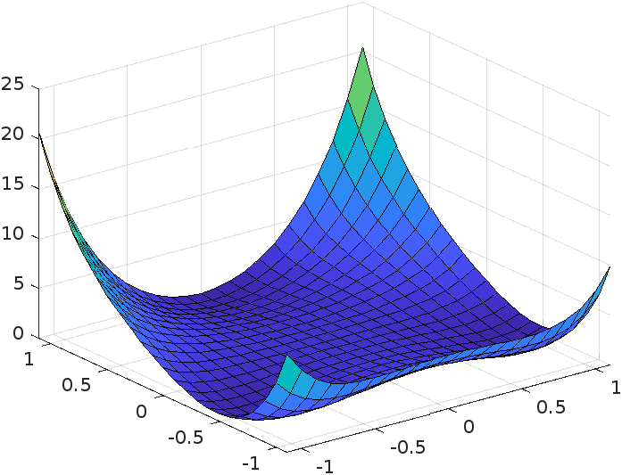
(a) Graph of the potential

(b) Contour lines of the potential

Figure 2: Graphics for the potential $W(u)=\absolutevalue{u-e^{i\pi\frac{3}{6}}}^{2}\absolutevalue{u-e^{i\pi\frac{7}{6}}}^{2}\absolutevalue{u-e^{i\pi\frac{11}{6}}}^{2}$

The existence of the function $W_{\mathrm{pert}}$ can then be seen by multiplying some suitable cutoff to $W$ which is equal to 1 on a sufficiently large ball.

As it is custom for parabolic partial differential equations, we view solutions of the Allen–Cahn equation (10) as maps from $[0,T]$ into some suitable function space and thus use the following definition.

Definition 3.1.

We say that a function

$$u_{\varepsilon}\in\mathrm{C}\left([0,T];\operatorname{L}^{2}\left(\operatorname{\mathbb{T}};\mathbb{R}^{N}\right)\right)\cap\operatorname{L}^{\infty}\left([0,T];\operatorname{W}^{1,2}(\operatorname{\mathbb{T}};\mathbb{R}^{N})\right)$$

is a weak solution of the Allen–Cahn equation (10) with parameter $\varepsilon>0$ and initial condition $u_{\varepsilon}^{0}\in\operatorname{L}^{2}(\operatorname{\mathbb{T}};\mathbb{R}^{N})$ if

1. the energy stays bounded, which means that

   $$\operatorname*{ess\,sup}_{0\leq t\leq T}\operatorname{E}_{\varepsilon}(u_{\varepsilon}(t))<\infty,$$ (16)

2. its weak time derivative satisfies

   $$\partial_{t}u_{\varepsilon}\in\operatorname{L}^{2}\left([0,T]\times\operatorname{\mathbb{T}};\mathbb{R}^{N}\right),$$ (17)

3. for almost every $t\in[0,T]$ and every

   $$\xi\in\operatorname{L}^{p}([0,T]\times\operatorname{\mathbb{T}};\mathbb{R}^{N})\cap\operatorname{W}^{1,2}([0,T]\times\operatorname{\mathbb{T}};\mathbb{R}^{N}),$$

   we have

   $$\int\left\langle\frac{1}{\varepsilon^{2}}\nabla W(u_{\varepsilon}(t))\,,\,\xi\right\rangle+\left\langle\nabla u_{\varepsilon}(t)\,,\,\nabla\xi\right\rangle+\left\langle\partial_{t}u_{\varepsilon}(t)\,,\,\xi\right\rangle\differential{x}=0,$$ (18)

4. the initial conditions are attained in the sense that $u_{\varepsilon}(0)=u_{\varepsilon}^{0}$.

Remark 3.2.

The exponent $p$ which appears in condition 3 is the same exponent as for the growth assumptions (12) and (13) of $W$. Moreover we note that given our setup, we automatically have $\nabla W(u_{\varepsilon})(t)\in\operatorname{L}^{p^{\prime}}(\operatorname{\mathbb{T}})$. In fact we can estimate

$$\absolutevalue{\nabla W(u_{\varepsilon})}^{p/(p-1)}\lesssim 1+\absolutevalue{u_{\varepsilon}}^{p}\lesssim 1+W(u),$$ (19)

which is integrable for almost every time $t$ since we assume that the energy stays bounded, thus the integral in equation (18) is well defined.

Moreover we already obtain $1/2$ Hölder-continuity in time from the embedding

$$\operatorname{W}^{1,2}\left([0,T];\operatorname{L}^{2}\left(\operatorname{\mathbb{T}};\mathbb{R}^{N}\right)\right)\hookrightarrow\operatorname{C}^{1/2}\left([0,T];\operatorname{L}^{2}\left(\operatorname{\mathbb{T}};\mathbb{R}^{N}\right)\right),$$ (20)

which follows from a generalized version of the fundamental theorem of calculus and Hölder’s inequality.

With Definition 3.1, we are able to state our existence result for a solution of the Allen–Cahn equation [LS18, Lemma 2.3] which uses De Giorgi’s minimizing movements scheme. Note moreover that one would expect even more regularity for a solution of the Allen–Cahn equation. In fact, it has been shown by De Mottoni and Schatzmann in [DS95] that in the scalar case, a solution u is smooth for positive times, at least for bounded initial data. Their Ansatz is a variation of parameters and the regularity then follows from the smoothing effect of the heat kernel.

Theorem 3.3.

Let $u^{0}\colon\operatorname{\mathbb{T}}\to\mathbb{R}^{N}$ be such that $\operatorname{E}_{\varepsilon}(u^{0})<\infty$. Then there exists a weak solution $u_{\varepsilon}$ to the Allen–Cahn equation (10) in the sense of Definition 3.1 with initial data $u^{0}$. Furthermore the solution satisfies the energy dissipation inequality

$$\operatorname{E}_{\varepsilon}(u_{\varepsilon}(t))+\int_{0}^{t}\int\varepsilon\absolutevalue{\partial_{t}u_{\varepsilon}}^{2}\differential{x}\differential{s}\leq\operatorname{E}_{\varepsilon}(u^{0})$$ (21)

for every $t\in[0,T]$. We additionally have $\partial_{i,j}^{2}u_{\varepsilon},\nabla W(u_{\varepsilon})\in\operatorname{L}^{2}([0,T]\times\operatorname{\mathbb{T}};\mathbb{R}^{N})$ for all $1\leq i,j\leq d$. In particular we can test the weak form (18) with $\partial_{i,j}^{2}u_{\varepsilon}$.

3.2 Convergence to an evolving partition

We now want to study of solutions to the Allen-Cahn equation (10) as $\varepsilon$ tends to zero. Let us first fix some notation. For a function $u=\sum_{i=1}^{P}\mathds{1}_{\Omega_{i}}\alpha_{i}$ with sets of finite perimeter $\Omega_{i}$ and the corresponding interfaces $\Sigma_{ij}\coloneqq\partial_{\ast}\Omega_{i}\cap\partial_{\ast}\Omega_{j}$, we define for a given continuous function $\varphi\in\operatorname{C}(\operatorname{\mathbb{T}})$ the energy measures by

$$\operatorname{E}_{\varepsilon}(u_{\varepsilon};\varphi) \coloneqq\int\varphi\left(\frac{1}{\varepsilon}W(u_{\varepsilon})+\frac{\varepsilon}{2}\absolutevalue{\nabla u_{\varepsilon}}^{2}\right)\differential{x}$$ (22)

and

$$\operatorname{E}(u;\varphi) \coloneqq\sum_{i<j}\sigma_{ij}\int_{\Sigma_{ij}}\varphi\differential{\operatorname{\mathcal{H}}^{d-1}}.$$ (23)

The latter is motivated through the perimeter functional introduced in Section 2.2.

One of the many difficulties in the vectorial case is that there is no easy choice of a primitive for $\sqrt{2W(u)}$ compared to the scalar case. This is crucial for the classic Modica–Mortola trick to obtain $\operatorname{BV}$-compactness. As a suitable replacement, we consider the geodesic distance defined as

$$\operatorname{\mathrm{d}_{\mathnormal{W}}}_{d}istance(u,v)$$

$$\coloneqq{} \inf\left\{\int_{0}^{1}\sqrt{2W(\gamma)}\absolutevalue{\dot{\gamma}}\differential{t}\,\colon\,\gamma\in\mathrm{C}^{1}\left([0,1];\mathbb{R}^{N}\right)\text{ with }\gamma(0)=u,\,\gamma(1)=v\right\}$$

motivated by Baldo in [Bal90]. This indeed defines a metric on $\mathbb{R}^{N}$: If we have $\operatorname{\mathrm{d}_{\mathnormal{W}}}_{d}istance(v,w)=0$, then by the continuity of $W$ and since it only has a discrete set of zeros, we may deduce that $v=w$. Symmetry can be seen by reversing a given path between two points and the triangle inequality follows from concatenation of two paths.

The surface tensions generated by $W$ are defined as

$$\sigma_{ij}\coloneqq\operatorname{\mathrm{d}_{\mathnormal{W}}}_{d}istance(\alpha_{i},\alpha_{j})$$ (24)

and as a consequence of $\operatorname{\mathrm{d}_{\mathnormal{W}}}_{d}istance$ being a metric satisfy the triangle inequality

$$\sigma_{ik}\leq\sigma_{ij}+\sigma_{jk}.$$

Furthermore $\sigma_{ij}$ is zero if and only if $i$ is equal to $j$ and by symmetry, $\sigma_{ij}$ is always the same as $\sigma_{ji}$.

Our replacement for the primitive of $\sqrt{2W}$ is given for $1\leq i\leq P$ by the geodesic distance function

$$\phi_{i}(u)\coloneqq\operatorname{\mathrm{d}_{\mathnormal{W}}}_{d}istance(\alpha_{i},u).$$

Our first obstacle is the regularity of the functions $\psi_{\varepsilon,i}\coloneqq\phi_{i}\circ u_{\varepsilon}$. A priori we only know that $\phi_{i}$ is locally Lipschitz continuous on $\mathbb{R}^{N}$ and thus differentiable almost everywhere. If $N=1$, this would already suffice to deduce that $\psi_{\varepsilon,i}$ is weakly differentiable. In higher dimensions however, $u$ could for example move along a hypersurface where $\phi_{i}$ could in theory be nowhere differentiable since the hypersurface is a Lebesgue nullset. This can be salvaged through the chain rule for distributional derivatives by Ambrosio and Dal Maso [AM90, Cor. 3.2]. Moreover we have the crucial inequality for its gradient given by

$$\absolutevalue{\nabla\psi_{i}(u)}\leq\sqrt{2W(u)}.$$ (25)

We then arrive at the following convergence result, see [LS18, Prop. 2.7].

Proposition 3.4.

Let $u_{\varepsilon}^{0}$ be well prepared initial data in the sense that

$$\lim_{\varepsilon\to 0}\operatorname{E}_{\varepsilon}(u_{\varepsilon}^{0})=\operatorname{E}(u^{0})\eqqcolon\operatorname{E}_{0}<\infty.$$

Then there exists for any sequence $\varepsilon\to 0$ some non-relabelled subsequence such that the solutions $u_{\varepsilon}$ of the Allen–Cahn equation (10) with initial conditions $u_{\varepsilon}^{0}$ converge in $\operatorname{L}^{1}\left((0,T)\times\operatorname{\mathbb{T}};\mathbb{R}^{N}\right)$ to some $u=\sum_{i=1}^{P}\chi_{i}\alpha_{i}$ with a partition

$$\chi\in\operatorname{BV}\left((0,T)\times\operatorname{\mathbb{T}};\{0,1\}^{P}\right).$$

Furthermore we have

$$\operatorname{E}(u(t))\leq\liminf_{\varepsilon\to 0}\operatorname{E}_{\varepsilon}(u_{\varepsilon}(t))\leq\operatorname{E}_{0}$$ (26)

for almost every time $0\leq t\leq T$ and $u$ attains the initial data $u^{0}$ continuously in $\operatorname{L}^{2}\left(\operatorname{\mathbb{T}};\mathbb{R}^{d}\right)$. Moreover for all $1\leq i\leq P$, the compositions $\psi_{\varepsilon,i}\coloneqq\phi_{i}\circ u_{\varepsilon}$ are uniformly bounded in $\operatorname{BV}((0,T)\times\operatorname{\mathbb{T}})$ and converge to $\psi_{i}\coloneqq\phi_{i}\circ u$ in $\operatorname{L}^{1}\left((0,T)\times\operatorname{\mathbb{T}}\right)$.

4 De Giorgi’s mean curvature flow

In this chapter, we build on the results of [LS18], but introduce a different solution concept for mean curvature flow, namely a De Giorgi type $\operatorname{BV}$-solution to mean curvature flow. A similar solution concept has been introduced in [LO16] and [LL21, Def. 1], but in the context of convergence of the thresholding scheme to mean curvature flow. Moreover, we will also compare it to the solution concept [HL21, Def. 1], which permits oriented varifolds to be solutions to mean curvature flow. This provides a more general notion of solution and is of use when the assumption of energy convergence falls away. See also the later discussion in Section 4.4.

4.1 Conditional convergence to De Giorgi’s mean curvature flow

In this section, we shall state our solution concept and prove convergence to the aforementioned.

Definition 4.1 (De Giorgi type $\operatorname{BV}$-solution to multiphase mean curvature flow).

Fix some finite time horizon $T<\infty$, a $(P\times P)$-matrix of surface tensions $\sigma$ and initial data $\chi^{0}\colon\operatorname{\mathbb{T}}\to\{0,1\}^{P}$ with $\operatorname{E}_{0}\coloneqq\operatorname{E}(\chi^{0})<\infty$ and $\sum_{i=1}^{P}\chi_{i}^{0}=1$ almost everywhere. We say that

$$\chi\in\operatorname{C}\left([0,T];\operatorname{L}^{2}\left(\operatorname{\mathbb{T}};\{0,1\}^{P}\right)\right)\cap\operatorname{BV}\left((0,T)\times\operatorname{\mathbb{T}};\{0,1\}^{P}\right)$$

with $\operatorname*{ess\,sup}_{0\leq t\leq T}\operatorname{E}(\chi)<\infty$ and $\sum_{i=1}^{P}\chi_{i}=\sum_{i=1}^{P}\mathds{1}_{\Omega_{i}}=1$ almost everywhere is a De Giorgi type $\operatorname{BV}$-solution to multiphase mean curvature flow with initial data $\chi^{0}$ and surface tensions $\sigma$ if the following holds.

1. For all $1\leq i\leq P$, there exists a normal velocity $V_{i}\in\operatorname{L}^{2}(\absolutevalue{\nabla\chi_{i}}\differential{t})$ such that

   $$\partial_{t}\chi_{i}=V_{i}\absolutevalue{\nabla\chi_{i}}\differential{t}$$

   holds in the distributional sense on $(0,T)\times\operatorname{\mathbb{T}}$.

2. There exist a mean curvature vector $H\in\operatorname{L}^{2}(\operatorname{E}(u;\cdot)\differential{t};\mathbb{R}^{d})$ which satisfies

   $$\sum_{1\leq i<j\leq P}\sigma_{ij}\int_{0}^{T}\int_{\Sigma_{ij}}\left\langle H\,,\,\xi\right\rangle\differential{\operatorname{\mathcal{H}}^{d-1}}\differential{t}$$

   $$={} -\sum_{1\leq i<j\leq P}\sigma_{ij}\int_{0}^{T}\int_{\Sigma_{ij}}\left\langle\mathrm{D}\xi\,,\,\mathrm{Id}-\nu_{i}\otimes\nu_{i}\right\rangle\differential{\operatorname{\mathcal{H}}^{d-1}}\differential{t}$$ (27)

   for all test vector fields $\xi\in\operatorname{C}_{\mathrm{c}}^{\infty}\left((0,T)\times\operatorname{\mathbb{T}};\mathbb{R}^{d}\right)$, where $\nu_{i}\coloneqq\nabla\chi_{i}/\absolutevalue{\nabla\chi_{i}}$ are the inner unit normals and $\Sigma_{ij}\coloneqq\partial_{\ast}\Omega_{i}\cap\partial_{\ast}\Omega_{j}$ is the $(i,j)$-th interface.

3. The partition $\chi$ satisfies a De Giorgi type optimal energy dissipation inequality in the sense that for almost every time $0<T^{\prime}<T$, we have

   $$\operatorname{E}(\chi(T^{\prime}))+\frac{1}{2}\sum_{1\leq i<j\leq P}\sigma_{ij}\int_{0}^{T^{\prime}}\int_{\Sigma_{ij}}V_{i}^{2}+\absolutevalue{H}^{2}\differential{\operatorname{\mathcal{H}}^{d-1}}\differential{t}\leq\operatorname{E}_{0}.$$ (28)

4. The initial data is attained in $\operatorname{C}\left([0,T];\operatorname{L}^{2}(\operatorname{\mathbb{T}})\right)$.

4.2 Localization estimates

Indeed, we obtain the existence of such solutions through a phase-field approximation with the Allen-Cahn equation as long as we assume the convergence of the integrated energies given by

$$\lim_{\varepsilon\to 0}\int_{0}^{T}\operatorname{E}_{\varepsilon}(u_{\varepsilon})\differential{t}=\int_{0}^{T}\operatorname{E}(u)\differential{t}.$$ (29)

A consequence of this is the equipartition of energies, already observed by Ilmanen in [Ilm93] for the scalar case under weaker assumptions using a comparison principle. The proof for the multiphase case can be found in [LS18, Lemma 2.11].

Lemma 4.2.

In the situation of Proposition 3.4 and under the energy convergence assumption (29), we have for any continuous function $\varphi\in\operatorname{C}(\operatorname{\mathbb{T}})$ that

$$\operatorname{E}(u;\varphi)=\lim_{\varepsilon\to 0}\operatorname{E}_{\varepsilon}(u_{\varepsilon};\varphi) =\lim_{\varepsilon\to 0}\int\varphi\sqrt{2W(u_{\varepsilon})}\absolutevalue{\nabla u_{\varepsilon}}\differential{x}$$

$$=\lim_{\varepsilon\to 0}\int\varphi\varepsilon\absolutevalue{\nabla u_{\varepsilon}}^{2}\differential{x}$$

$$=\lim_{\varepsilon\to 0}\int\varphi\frac{1}{\varepsilon}2W(u_{\varepsilon})\differential{x}$$

for almost every time $0\leq t\leq T$.

In order to prove convergence, we want to reduce the multiphase case to the two-phase case. The central idea here is to cover the flat torus with a suitable collection of balls. Then we argue that, up to a small error, we can choose for each ball a pair of majority phases $(i,j)$ such that the partition looks like a two-phase mean curvature flow on the ball, see Figure 3.

Figure 3: Localization of multiphase mean curvature flow. For the green balls, we choose the majority phase (2,3), for the blue ones (1,3) and for the yellow balls (3,4). The red balls however give us an error.

To formulate this rigorously let $r>0$ and define the covering $\mathcal{B}_{r}$ of the flat torus by

$$\mathcal{B}_{r}\coloneqq\left\{B_{r}(c)\,\colon\,c\in\mathcal{L}_{r}\right\},$$

where the set of centers $\mathcal{L}_{r}$ is given by $\mathcal{L}_{r}\coloneqq\operatorname{\mathbb{T}}\cap(r/\sqrt{d})\mathbb{Z}^{d}$. Moreover let $\rho_{B}$ be a smooth cutoff for the ball $B$ with support in the ball with the same center, but double the radius.

Additionally to choosing a majority phase, we can also argue that along the chosen majority phase, we have a local flatness. Thus we may approximate the inner unit normal up to an arbitrarily small error by a constant unit vector. This is captured by the following lemma found in [LO16]. The proof is based on De Giorgi’s structure theorem for sets of finite perimeter.

Lemma 4.3.

For every $\delta>0$ and every partition $\chi\colon\operatorname{\mathbb{T}}\to\{0,1\}^{P}$ such that $\chi_{i}\in\operatorname{BV}(\operatorname{\mathbb{T}})$ holds for all $1\leq i\leq P$, there exist some $r_{0}>0$ such that for all $0<r<r_{0}$, we find for every ball $B\in\mathcal{B}_{r}$ some unit vector $\nu_{B}$ such that

$$\sum_{B\in\mathcal{B}_{r}}\min_{i\neq j}\int\rho_{B}\absolutevalue{\nu_{i}-\nu_{B}}^{2}\absolutevalue{\nabla\chi_{i}}+\int\rho_{B}\absolutevalue{\nu_{j}+\nu_{B}}^{2}\absolutevalue{\nabla\chi_{j}}+\sum_{k\notin\{i,j\}}\int\rho_{B}\absolutevalue{\nabla\chi_{k}}$$

$$\lesssim{} \delta\operatorname{E}(\chi).$$

Note that summing $\absolutevalue{\nabla\chi_{k}}$ over all $k\notin\{i,j\}$ corresponds to summing over all interfaces which are not the $(i,j)$-th interface, see also [Bal90]. Moreover the second summand is redundant. In fact the last summand provides us with a localization on the $(i,j)$-th interface, on which we have $\nu_{i}=-\nu_{j}$. However it is convenient to keep it so that we do not have to repeat this argument.

Remark 4.4.

This localization estimate also implies the smallness of

$$\sum_{B\in\mathcal{B}_{r}}\min_{i}\absolutevalue{\operatorname{E}(\chi;\rho_{B})-\int\rho_{B}\absolutevalue{\nabla\psi_{i}}}=\sum_{B\in\mathcal{B}_{r}}\operatorname{E}(\chi;\rho_{B})-\max_{i}\int\rho_{B}\absolutevalue{\nabla\psi_{i}}$$ (30)

in the same sense as in the above Lemma 4.3. Notice that the equality (30) follows from

$$\absolutevalue{\nabla\psi_{i}}=\sum_{1\leq k<l\leq P}\absolutevalue{\sigma_{ik}-\sigma_{il}}\operatorname{\mathcal{H}}^{d-1}\llcorner_{\Sigma_{kl}}\leq\operatorname{E}(\chi;\cdot),$$ (31)

where we remind that $\psi_{i}\coloneqq\phi_{i}\circ u$. The smallness follows since we have for every $i\neq j$ that

$$\operatorname{E}(\chi;\rho_{B})-\int\rho_{B}\absolutevalue{\nabla\psi_{i}}$$

$$={} \sum_{1\leq k<l\leq P}\sigma_{kl}\int_{\Sigma_{kl}}\rho_{B}\differential{\operatorname{\mathcal{H}}^{d-1}}-\sum_{1\leq k<l\leq P}\absolutevalue{\sigma_{ik}-\sigma_{il}}\int_{\Sigma_{kl}}\rho_{B}\differential{\operatorname{\mathcal{H}}^{d-1}}$$

$$={} \sum_{\begin{subarray}{c}1\leq k<l\leq P\\ (k,l)\neq(i,j)\end{subarray}}\left(\sigma_{kl}-\absolutevalue{\sigma_{ik}-\sigma_{il}}\right)\int_{\Sigma_{kl}}\rho_{B}\differential{\operatorname{\mathcal{H}}^{d-1}}$$

$$\lesssim{} \sum_{k\notin\{i,j\}}\int\rho_{B}\absolutevalue{\nabla\chi_{k}}.$$

Thus we can estimate the error by the last summand of the error in Lemma 4.3.

4.3 Conditional convergence of Allen–Cahn equations to De Giorgi’s multiphase mean curvature flow

We are now in the position to prove the desired conditional convergence result.

Theorem 4.5.

Let $W\colon\mathbb{R}^{N}\to[0,\infty)$ be a smooth multiwell potential satisfying the assumptions (12)-(15). Let $T<\infty$ be an arbitrary finite time horizon. Let $u_{\varepsilon}^{0}\colon\operatorname{\mathbb{T}}\to\mathbb{R}^{N}$ be a sequence of initial data approximating a partition $\chi^{0}\in\operatorname{BV}\left(\operatorname{\mathbb{T}};\{0,1\}^{P}\right)$ in the sense that $u_{\varepsilon}^{0}\to u^{0}=\sum_{1\leq i\leq P}\chi_{i}^{0}\alpha_{i}$ holds pointwise almost everywhere and

$$\operatorname{E}_{0}\coloneqq\operatorname{E}(\chi^{0})=\lim_{\varepsilon\to 0}\operatorname{E}_{\varepsilon}(u_{\varepsilon}^{0})<\infty.$$

Then we have for some subsequence of solutions $u_{\varepsilon}$ to the Allen–Cahn equation (10) with initial datum $u_{\varepsilon}^{0}$ that there exists a time-dependent partition $\chi$ with

$$\chi\in\operatorname{BV}\left((0,T)\times\operatorname{\mathbb{T}};\{0,1\}^{P}\right)$$

and $\chi\in\operatorname{C}\left([0,T];\operatorname{L}^{2}\left(\operatorname{\mathbb{T}};\{0,1\}^{P}\right)\right)$ such that $u_{\varepsilon}$ converges to $u\coloneqq\sum_{1\leq i\leq P}\chi_{i}\alpha_{i}$ in $\operatorname{L}^{1}\left((0,T)\times\operatorname{\mathbb{T}};\mathbb{R}^{N}\right)$. Moreover $u$ attains the initial data $u^{0}$ continuously in $\operatorname{L}^{2}\left(\operatorname{\mathbb{T}};\mathbb{R}^{N}\right)$.

If we additionally assume that the time-integrated energies converge (29), then $\chi$ is a De Giorgi type $\operatorname{BV}$-solution to multiphase mean curvature flow in the sense of Definition 4.1.

Proof.

Proposition 3.4 already provides us with all claims except the last. The idea of the proof is that we already have an optimal energy dissipation inequality for the Allen–Cahn equation given by (21). If we additionally use the Allen–Cahn equation once, we arrive at the De Giorgi type optimal energy dissipation inequality given by

$$\operatorname{E}_{\varepsilon}(u_{\varepsilon}(T^{\prime}))+\frac{1}{2}\int_{0}^{T^{\prime}}\int\varepsilon\absolutevalue{\partial_{t}u_{\varepsilon}}^{2}+\frac{1}{\varepsilon}\absolutevalue{\varepsilon\Delta u_{\varepsilon}-\frac{1}{\varepsilon}\nabla W(u_{\varepsilon})}^{2}\differential{x}\differential{t}\leq\operatorname{E}_{\varepsilon}(u_{\varepsilon}^{0}).$$

Our hope is that as $\varepsilon$ tends to zero, we can pass to the optimal energy dissipation inequality (28) for $\chi$ through lower semicontinuity. Since we assume the convergence of the initial energies and energy convergence for almost every time, the only terms we have to care about are the velocity and curvature term. The desired lower semicontinuity of the velocity term reads

$$\liminf_{\varepsilon\to 0}\frac{1}{2}\int_{0}^{T^{\prime}}\int\varepsilon\absolutevalue{\partial_{t}u_{\varepsilon}}^{2}\differential{x}\differential{t}\geq\frac{1}{2}\sum_{i<j}\sigma_{ij}\int_{0}^{T^{\prime}}\int_{\Sigma_{ij}}V_{i}^{2}\differential{\operatorname{\mathcal{H}}^{d-1}}\differential{t}$$ (32)

and the lower semicontinuity of the curvature term is given by

$$\liminf_{\varepsilon\to 0}\frac{1}{2}\int_{0}^{T^{\prime}}\int\frac{1}{\varepsilon}\absolutevalue{\varepsilon\Delta u_{\varepsilon}-\frac{1}{\varepsilon}\nabla W(u_{\varepsilon})}^{2}\differential{x}\differential{t}$$

$$\geq{} \frac{1}{2}\sum_{i<j}\sigma_{ij}\int_{0}^{T^{\prime}}\int_{\Sigma_{ij}}\absolutevalue{H}^{2}\differential{\operatorname{\mathcal{H}}^{d-1}}\differential{t}.$$ (33)

The existence of square integrable distributional normal velocities has been proven in [LS18, Prop. 2.10]. Moreover we have to show the existence of the mean curvature vector $H$. We could cheat in this step and simply use that by the main result [LS18, Thm. 1.2], we already know that the tangential divergence applied to $\xi$ is given by the velocity. In other words, that we already have $V_{i}\nu_{i}=-H$ on $\Sigma_{ij}$. But we want to present a more direct approach.

Consider the linear functional

$$L(\xi)\coloneqq-\sum_{1\leq i<j\leq P}\sigma_{ij}\int_{0}^{T}\int_{\Sigma_{ij}}\left\langle\mathrm{D}\xi\,,\,\mathrm{Id}-\nu_{i}\otimes\nu_{i}\right\rangle\differential{\operatorname{\mathcal{H}}^{d-1}}\differential{t}$$

defined on test vector fields $\xi$. Then $L$ is bounded with respect to the $\operatorname{L}^{2}$-norm on $(0,T)\times\operatorname{\mathbb{T}}$ equipped with the measure $\operatorname{E}(u;\cdot)\differential{t}$ since by the convergence of the curvature term observed in [LS18, Prop. 3.1], we have

$$\absolutevalue{L(\xi)}$$

$$={} \lim_{\varepsilon\to 0}\absolutevalue{-\int_{0}^{T}\int\left\langle\varepsilon\Delta u_{\varepsilon}-\frac{1}{\varepsilon}\nabla W(u_{\varepsilon})\,,\,\mathrm{D}u_{\varepsilon}\xi\right\rangle\differential{x}\differential{t}}$$

$$\leq{} \liminf_{\varepsilon\to 0}\left(\int_{0}^{T}\int\frac{1}{\varepsilon}\absolutevalue{\varepsilon\Delta u_{\varepsilon}-\frac{1}{\varepsilon}\nabla W(u_{\varepsilon})}^{2}\differential{x}\differential{t}\right)^{1/2}\left(\int_{0}^{T}\int\varepsilon\absolutevalue{\mathrm{D}u_{\varepsilon}\xi}^{2}\differential{x}\differential{t}\right)^{1/2}$$

$$\leq{} \liminf_{\varepsilon\to 0}\left(\int_{0}^{T}\int\varepsilon\absolutevalue{\partial_{t}u_{\varepsilon}}^{2}\differential{x}\differential{t}\right)^{1/2}\left(\int_{0}^{T}\int\varepsilon\absolutevalue{\nabla u_{\varepsilon}}^{2}\absolutevalue{\xi}^{2}\differential{x}\differential{t}\right)^{1/2}.$$

The first factor stays uniformly bounded due to the energy dissipation inequality (21), and by the equipartition of energies (Lemma 4.2), the second factor converges to the $\operatorname{L}^{2}$-norm of $\xi$ with respect to the energy measure, proving our claim. Therefore we can extend the functional to the square integrable functions with respect to the energy measure. By Riesz representation theorem we obtain the existence of the desired mean curvature vector $H$.

Let us now consider the lower semicontinuity of the curvature term, which in particular yields a sharp version of the previous estimate. Let again $\xi$ be some test vector field. Then for all $\varepsilon>0$ and some fixed time, we have by Young’s inequality

$$\liminf_{\varepsilon\to 0}\frac{1}{2}\int\frac{1}{\varepsilon}\absolutevalue{\varepsilon\Delta u_{\varepsilon}-\frac{1}{\varepsilon}\nabla W(u_{\varepsilon})}^{2}\differential{x}$$

$$\geq{} \liminf_{\varepsilon\to 0}\int\left\langle\varepsilon\Delta u_{\varepsilon}-\frac{1}{\varepsilon}\nabla W(u_{\varepsilon})\,,\,\mathrm{D}u_{\varepsilon}\xi\right\rangle\differential{x}-\frac{1}{2}\int\varepsilon\absolutevalue{\mathrm{D}u_{\varepsilon}\xi}^{2}\differential{x}$$

$$\geq{} \liminf_{\varepsilon\to 0}\int\left\langle\varepsilon\Delta u_{\varepsilon}-\frac{1}{\varepsilon}\nabla W(u_{\varepsilon})\,,\,\mathrm{D}u_{\varepsilon}\xi\right\rangle\differential{x}-\limsup_{\varepsilon\to 0}\frac{1}{2}\int\varepsilon\absolutevalue{\mathrm{D}u_{\varepsilon}}^{2}\absolutevalue{\xi}^{2}$$

$$\geq{} -\operatorname{E}\left(\chi;\left\langle H\,,\,\xi\right\rangle\right)-\frac{1}{2}\operatorname{E}\left(\chi;\absolutevalue{\xi}^{2}\right).$$

Here the last inequality is due to the above mentioned convergence of the curvature term and the equipartition of energies Lemma 4.2. Since this inequality holds for any test vector field, we may take a sequence of test vector fields $\xi_{n}$ satisfying

$$\lim_{n\to\infty}\norm{\xi_{n}+H}_{\operatorname{L}^{2}\left(\operatorname{\mathbb{T}},\operatorname{E}(\chi;\cdot);\mathbb{R}^{d}\right)}=0.$$

This then yields the desired inequality (4.3) by applying Fatou’s lemma.

In principle the proof is now already done, since the main result by Laux and Simon already gives us that for almost every time $t$, we have $V_{i}\nu_{i}=-H$ on $\Sigma_{i,j}$ $\operatorname{\mathcal{H}}^{d-1}$-almost everywhere. We instead want to present another proof which directly proves the lower semicontinuity of the velocity term and may leave more room for future generalizations.

Let us first consider the two-phase case $N=1$ and $P=2$. By a similar duality argument as for the lower semicontinuity of the curvature term, we compute that for every test function $\varphi$, we have

$$\liminf_{\varepsilon\to 0}\frac{1}{2}\int_{0}^{T}\int\varepsilon\absolutevalue{\partial_{t}u_{\varepsilon}}^{2}\differential{x}\differential{t}$$

$$\geq{} \liminf_{\varepsilon\to 0}\int_{0}^{T}\int\partial_{t}u_{\varepsilon}\phi^{\prime}(u_{\varepsilon})\varphi\differential{x}\differential{t}-\frac{1}{2}\int_{0}^{T}\int\frac{1}{\varepsilon}\left(\phi^{\prime}(u_{\varepsilon})\varphi\right)^{2}\differential{x}\differential{t}$$

$$={} \liminf_{\varepsilon\to 0}\int_{0}^{T}\int\partial_{t}\psi_{\varepsilon}\varphi\differential{x}\differential{t}-\frac{1}{2}\int_{0}^{T}\int\frac{1}{\varepsilon}2W(u_{\varepsilon})\varphi^{2}\differential{x}\differential{t}$$

$$={} \sigma\int_{0}^{T}\int_{\Sigma}\varphi V\differential{\operatorname{\mathcal{H}}^{d-1}}\differential{t}-\frac{1}{2}\sigma\int_{0}^{T}\int_{\Sigma}\varphi^{2}\differential{\operatorname{\mathcal{H}}^{d-1}}\differential{t}.$$

Here the last equality uses the weak convergence of $\partial_{t}(\phi\circ u_{\varepsilon})=\partial_{t}\psi_{\varepsilon}$ to $\partial_{t}(\phi\circ u)=\partial_{t}\psi=\sigma V\absolutevalue{\nabla\chi}\differential{t}$ given by Proposition 3.4 for the first summand and the equipartition of energies (Lemma 4.2) for the second summand. Since the inequality holds for any test function $\varphi$, we may plug in a sequence of test functions $\varphi_{n}$ satisfying

$$\lim_{n\to\infty}\norm{\varphi_{n}-V}_{\operatorname{L}^{2}\left((0,T)\times\operatorname{\mathbb{T}},\operatorname{\mathcal{H}}^{d-1}\llcorner_{\Sigma}\differential{t}\right)}=0$$

and thereby obtain the desired inequality (32).

For the multiphase case, we do not find an immediate generalization of this proof, but rather have to work with a localization argument in order to obtain a reduction to the two-phase case.

For a localization in time, let $\delta>0$ and $0=T_{0}<T_{1}<\dotsc<T_{K}=T^{\prime}$ be a partition of $[0,T^{\prime}]$. Let $(g_{k})_{k=1,\dotsc,K}$ be a partition of unity with respect to the intervals $\left((T_{k-1}-\delta,T_{k}+\delta)\right)_{1\leq k\leq K}$, let $r>0$ and $\eta_{B}$ a partition of unity in space as in Lemma 4.3. Moreover we fix some $R>0$. Then we estimate by Young’s inequality

$$\liminf_{\varepsilon\to 0}\frac{1}{2}\int_{0}^{T}\int\varepsilon\absolutevalue{\partial_{t}u_{\varepsilon}}^{2}\differential{x}\differential{t}$$

$$={} \liminf_{\varepsilon\to 0}\sum_{k=1}^{K}\sum_{B\in\mathcal{B}_{r}}\frac{1}{2}\int_{0}^{T}\int g_{k}\eta_{B}\varepsilon\absolutevalue{\partial_{t}u_{\varepsilon}}^{2}\differential{x}\differential{t}$$

$$\geq{} \liminf_{\varepsilon\to 0}\sum_{k=1}^{K}\sum_{B\in\mathcal{B}_{r}}\max_{1\leq i\leq P}\sup_{\begin{subarray}{c}\varphi\in\operatorname{C}_{\mathrm{c}}^{\infty}\left((0,T)\times\operatorname{\mathbb{T}}\right)\\ \absolutevalue{\varphi}\leq R\end{subarray}}\int_{0}^{T}\int g_{k}\eta_{B}\left\langle\nabla\phi_{i}(u_{\varepsilon})\,,\,\partial_{t}u_{\varepsilon}\right\rangle\varphi\differential{x}\differential{t}$$

$$\qquad\qquad\qquad\qquad\qquad\qquad\qquad\quad-\frac{1}{2}\int_{0}^{T}\int g_{k}\eta_{B}\frac{1}{\varepsilon}\absolutevalue{\nabla\phi_{i}(u_{\varepsilon})}^{2}\varphi^{2}\differential{x}\differential{t}.$$

We identify via the chain rule that $\left\langle\nabla\phi_{i}(u_{\varepsilon})\,,\,\partial_{t}u_{\varepsilon}\right\rangle=\partial_{t}\psi_{\varepsilon,i}$ and moreover remember $\absolutevalue{\nabla\phi_{i}}\leq\sqrt{2W}$ from inequality (25). We pull the limit inferior inside the double sum and the suprema and thus obtain that this term can be estimated from below by

$$\sum_{k=1}^{K}\sum_{B\in\mathcal{B}_{r}}\max_{1\leq i\leq P}\sup_{\begin{subarray}{c}\varphi\in\operatorname{C}_{\mathrm{c}}^{\infty}\left((0,T)\times\operatorname{\mathbb{T}}\right)\\ \absolutevalue{\varphi}\leq R\end{subarray}}\liminf_{\varepsilon\to 0}\int_{0}^{T}\int g_{k}\eta_{B}\varphi\partial_{t}\psi_{\varepsilon,i}$$

$$\qquad\qquad\qquad\qquad\qquad\quad\;\;-\limsup_{\varepsilon\to 0}\frac{1}{2}\int_{0}^{T}\int g_{k}\eta_{B}\frac{2}{\varepsilon}W(u_{\varepsilon})\varphi^{2}\differential{x}\differential{t}$$

$$={} \sum_{k=1}^{K}\sum_{B\in\mathcal{B}_{r}}\max_{1\leq i\leq P}\sup_{\begin{subarray}{c}\varphi\in\operatorname{C}_{\mathrm{c}}^{\infty}\left((0,T)\times\operatorname{\mathbb{T}}\right)\\ \absolutevalue{\varphi}\leq R\end{subarray}}\int_{0}^{T}\int g_{k}\eta_{B}\varphi\partial_{t}\psi_{i}-\frac{1}{2}\int_{0}^{T}\operatorname{E}\left(\chi;g_{k}\eta_{B}\varphi^{2}\right)\differential{t}.$$

For the equality we used the equipartition of energies Lemma 4.2 and the $\operatorname{L}^{1}$-convergence of $\psi_{\varepsilon,i}$ to $\psi_{i}$ given by Proposition 3.4. By adding zero, we get

$$\int_{0}^{T}\int g_{k}\eta_{B}\varphi\partial_{t}\psi_{i}\differential{x}\differential{t}-\frac{1}{2}\int_{0}^{T}\operatorname{E}\left(\chi;g_{k}\eta_{B}\varphi^{2}\right)\differential{t}$$

$$={} \sum_{j=1}^{P}\left(\sigma_{ij}\int_{0}^{T}\int g_{k}\eta_{B}\varphi V_{j}\absolutevalue{\nabla\chi_{j}}\differential{t}-\frac{1}{2}\sigma_{ij}\int_{0}^{T}\int g_{k}\eta_{B}\varphi^{2}\absolutevalue{\nabla\chi_{j}}\differential{t}\right)$$

$$-\frac{1}{2}\int_{0}^{T}\left(\operatorname{E}\left(\chi;g_{k}\eta_{B}\varphi^{2}\right)-\int g_{k}\eta_{B}\varphi^{2}\absolutevalue{\nabla\psi_{i}}\right)\differential{t}.$$

Since no derivative has fallen on $g_{k}$, we may send $\delta$ to zero and obtain by the dominated convergence theorem that we can replace $g_{k}$ by $\mathds{1}_{(T_{k-1},T_{k})}$. We thus end up with a good summand consisting of

$$\sum_{k=1}^{K}\sum_{B\in\mathcal{B}_{r}}\max_{1\leq i\leq P}\sup_{\begin{subarray}{c}\varphi\in\operatorname{C}_{\mathrm{c}}^{\infty}\left((0,T)\times\operatorname{\mathbb{T}}\right)\\ \absolutevalue{\varphi}\leq R\end{subarray}}\sum_{j=1}^{P}\sigma_{ij}\int_{T_{k-1}}^{T_{k}}\int\eta_{B}\varphi\left(V_{j}-\frac{1}{2}\varphi\right)\absolutevalue{\nabla\chi_{j}}\differential{t}$$ (34)

and an error summand given by

$$\sum_{k=1}^{K}\sum_{B\in\mathcal{B}_{r}}\max_{1\leq i\leq P}\sup_{\begin{subarray}{c}\varphi\in\operatorname{C}_{\mathrm{c}}^{\infty}\left((0,T)\times\operatorname{\mathbb{T}}\right)\\ \absolutevalue{\varphi}\leq R\end{subarray}}-\frac{1}{2}\int_{T_{k-1}}^{T_{k}}\left(\operatorname{E}\left(\chi;\eta_{B}\varphi^{2}\right)-\int\eta_{B}\varphi^{2}\absolutevalue{\nabla\psi_{i}}\right)\differential{t}$$

$$\geq{} \sum_{k=1}^{K}\sum_{B\in\mathcal{B}_{r}}\max_{1\leq i\leq P}-\frac{R^{2}}{2}\int_{T_{k-1}}^{T_{k}}\left(\operatorname{E}\left(\chi;\eta_{B}\right)-\int\eta_{B}\absolutevalue{\nabla\psi_{i}}\right)\differential{t},$$ (35)

where we used $\absolutevalue{\nabla\psi_{i}}\leq\operatorname{E}(\chi,\cdot)$. We choose a majority phase $(i,j)$ and estimate the summands of (34) from below using

$$\max_{1\leq i\leq P}\sup_{\begin{subarray}{c}\varphi\in\operatorname{C}_{\mathrm{c}}^{\infty}\left((0,T)\times\operatorname{\mathbb{T}}\right)\\ \absolutevalue{\varphi}\leq R\end{subarray}}\sum_{j=1}^{P}\sigma_{ij}\int_{T_{k-1}}^{T_{k}}\int\eta_{B}\varphi\left(V_{j}-\frac{1}{2}\varphi\right)\absolutevalue{\nabla\chi_{j}}\differential{t}$$

$$\geq{} \max_{i<j}\sup_{\begin{subarray}{c}\varphi\in\operatorname{C}_{\mathrm{c}}^{\infty}\left((0,T)\times\operatorname{\mathbb{T}}\right)\\ \absolutevalue{\varphi}\leq R\end{subarray}}\sigma_{ij}\int_{T_{k-1}}^{T_{k}}\int\eta_{B}\varphi\left(V_{j}-\frac{1}{2}\varphi\right)\absolutevalue{\nabla\chi_{j}}\differential{t}$$

$$\qquad\qquad\qquad\qquad-C\sum_{l\notin\{i,j\}}\int_{T_{k-1}}^{T_{k}}\int\eta_{B}\left(R\absolutevalue{V_{l}}+R^{2}\right)\absolutevalue{\nabla\chi_{l}}\differential{t}.$$ (36)

Concerning the error term, we have by Remark 4.4 that

$$\frac{R^{2}}{2}\int_{T_{k-1}}^{T_{k}}\operatorname{E}\left(\chi;\eta_{B}\right)-\int\eta_{B}\absolutevalue{\nabla\psi_{i}}\differential{t}\lesssim R^{2}\sum_{l\notin\{i,j\}}\int_{T_{k-1}}^{T_{k}}\int\eta_{B}\absolutevalue{\nabla\chi_{l}}\differential{t},$$

which enables us to absorb the error (35) into the error term (36). By applying Young’s inequality, we get that for every parameter $\alpha\in(0,1)$, we have

$$\int_{T_{k-1}}^{T_{k}}\int\eta_{B}R\absolutevalue{V_{l}}\absolutevalue{\nabla\chi_{l}}\differential{t}\lesssim\alpha\int_{T_{k-1}}^{T_{k}}\int\eta_{B}V_{l}^{2}\absolutevalue{\nabla\chi_{l}}\differential{t}+\frac{R^{2}}{\alpha}\int_{T_{k-1}}^{T_{k}}\int\eta_{B}\absolutevalue{\nabla\chi_{l}}\differential{t}.$$

Collecting our estimates, we end up with an error term which can be estimated from below up to a constant by

$$-\alpha\sum_{l=1}^{P}\int_{0}^{T}\int V_{l}^{2}\absolutevalue{\nabla\chi_{l}}\differential{t}-\frac{R^{2}}{\alpha}\sum_{k=1}^{K}\sum_{B\in\mathcal{B}_{r}}\max_{i<j}\sum_{l\notin\{i,j\}}\int_{T_{k-1}}^{T_{k}}\int\eta_{B}\absolutevalue{\nabla\chi_{l}}\differential{t}.$$

Moreover, we can choose for fixed $k,B$ and tuple $(i,j)$ a sequence of test functions $\varphi_{n}$ with $\absolutevalue{\varphi_{n}}\leq R$ which converge to $V_{j}\mathds{1}_{\absolutevalue{V_{j}\leq R}}$ in the sense that

$$\lim_{n\to\infty}\norm{\varphi_{n}-V_{j}\mathds{1}_{\absolutevalue{V_{j}}\leq R}}_{\operatorname{L}^{2}\left((T_{k-1},T_{k})\times\operatorname{\mathbb{T}},\absolutevalue{\nabla\chi_{j}}\differential{t}\right)}=0.$$

Combining these three arguments, we arrive at the estimate

$$\liminf_{\varepsilon\to 0}\frac{1}{2}\int_{0}^{T}\int\varepsilon\absolutevalue{\partial_{t}u_{\varepsilon}}^{2}\differential{x}\differential{t}$$

$$\geq{} -C\alpha\sum_{1\leq l\leq P}\int_{0}^{T}\int V_{l}^{2}\absolutevalue{\nabla\chi_{l}}\differential{t}$$

$$+\sum_{k=1}^{K}\sum_{B\in\mathcal{B}_{r}}\max_{i<j}\int_{T_{k-1}}^{T_{k}}\frac{\sigma_{ij}}{2}\int\eta_{B}\absolutevalue{V_{j}\mathds{1}_{\absolutevalue{V_{j}}\leq R}}^{2}\absolutevalue{\nabla\chi_{j}}-C\frac{R^{2}}{\alpha}\sum_{l\notin\{i,j\}}\int\eta_{B}\absolutevalue{\nabla\chi_{l}}\differential{t}$$

for every parameter $\alpha\in(0,1)$. We choose partitions whose width tends to zero and which are contained in each other. By the monotone convergence theorem and using Lebesgue points, we can pull the maximum inside the time integral to obtain

$$\liminf_{\varepsilon\to 0}\frac{1}{2}\int_{0}^{T}\int\varepsilon\absolutevalue{\partial_{t}u_{\varepsilon}}^{2}\differential{x}\differential{t}$$

$$\geq{} -\alpha C\sum_{1\leq l\leq P}\int_{0}^{T}\int V_{l}^{2}\absolutevalue{\nabla\chi_{l}}\differential{t}$$

$$+\int_{0}^{T}\sum_{B\in\mathcal{B}_{r}}\max_{i<j}\frac{\sigma_{ij}}{2}\int\eta_{B}\absolutevalue{V_{j}\mathds{1}_{\absolutevalue{V_{j}}\leq R}}^{2}\absolutevalue{\nabla\chi_{j}}-C\frac{R^{2}}{\alpha}\sum_{l\notin\{i,j\}}\int\eta_{B}\absolutevalue{\nabla\chi_{l}}\differential{t}$$

$$\geq{} \frac{1}{2}\sum_{1\leq i<j\leq P}\sigma_{ij}\int_{0}^{T}\int_{\Sigma_{ij}}V_{i}^{2}\mathds{1}_{\absolutevalue{V_{i}}\leq R}\differential{\operatorname{\mathcal{H}}^{d-1}}\differential{t}$$

$$-C\left(\alpha\sum_{1\leq l\leq P}\int_{0}^{T}\int V_{l}^{2}\absolutevalue{\nabla\chi_{l}}\differential{t}+\frac{R^{2}}{\alpha}\int_{0}^{T}\sum_{B\in\mathcal{B}_{r}}\min_{i\neq j}\sum_{k\notin\{i,j\}}\int\eta_{B}\absolutevalue{\nabla\chi_{k}}\differential{t}\right).$$

We first send $r\to 0$ and then $\alpha\to 0$ . By the localization result Lemma 4.3 we thus obtain that for all $R>0$

$$\liminf_{\varepsilon\to 0}\frac{1}{2}\int_{0}^{T}\int\varepsilon\absolutevalue{\partial_{t}u_{\varepsilon}}^{2}\differential{x}\differential{t}\geq\frac{1}{2}\sum_{1\leq i<j\leq P}\sigma_{ij}\int_{0}^{T}\int_{\Sigma_{ij}}V_{i}^{2}\mathds{1}_{\absolutevalue{V_{i}}\leq R}\differential{\operatorname{\mathcal{H}}^{d-1}}\differential{t}.$$

Therefore the lower semicontinuity of the velocity term now follows from the monotone convergence theorem. ∎

4.4 De Giorgi type varifold solutions for mean curvature flow

Up until this point, we have always made the crucial assumption of energy convergence (29) for our proofs. However this is usually a very strong assumption. One thing which could go wrong is for example illustrated in Figure 4. There we see that two approximate interfaces of the first and second phase collapse as $\varepsilon$ tends to zero. This results in a loss of energy since the measure theoretic boundary of a set with finite perimeter does not see such lines.

(a) $1>\varepsilon>0$

(b) $1\gg\varepsilon>0$

(c) $\varepsilon=0$

Figure 4: Profile of the solution $u_{\varepsilon}$ as $\varepsilon$ tends to zero.

We now introduce the solution concept by Hensel and Laux in [HL21] which tackles this issue. For the two-phase case, the definition is as follows.

Definition 4.6 (De Giorgi type varifold solution for two-phase mean curvature flow).

Let $T<\infty$ be an arbitrary finite time horizon and let $\mu=\operatorname{\mathcal{L}}^{1}\otimes(\mu_{t})_{t\in(0,T)}$ be a family of oriented varifolds $\mu_{t}\in\mathcal{M}\left(\operatorname{\mathbb{T}}\times\mathbb{S}^{d-1}\right)$ for $t\in(0,T)$ such that $t\mapsto\int_{\operatorname{\mathbb{T}}\times\mathbb{S}^{d-1}}\eta(t,x,p)\differential\mu_{t}(x,p)$ is measurable for all $\eta\in\operatorname{L}^{1}\left((0,T);\operatorname{C}\left(\operatorname{\mathbb{T}},\mathbb{S}^{d-1}\right)\right)$. Consider also a family $A=(A_{t})_{t\in(0,T)}$ of subsets of $\operatorname{\mathbb{T}}$ with finite perimeter such that the associated indicator function $\chi(x,t)\coloneqq\chi_{A_{t}}(x)$ is in the space $\operatorname{L}^{\infty}\left((0,T);\operatorname{BV}(\operatorname{\mathbb{T}};\{0,1\})\right)$. Let $\sigma>0$ be a surface tension constant.

Given an initial energy $\omega^{0}\in\mathcal{M}\left(\operatorname{\mathbb{T}}\right)$ and initial data $\chi^{0}\in\operatorname{BV}\left(\operatorname{\mathbb{T}};\{0,1\}\right)$, we call the pair $(\mu,\chi)$ a De Giorgi type varifold solution to two-phase mean curvature flow with initial data $(\omega^{0},\chi^{0})$ if the following holds.

1. (Existence of a normal speed) Writing $\mu_{t}=\omega_{t}\otimes(\lambda_{t,x})_{x\in\operatorname{\mathbb{T}}}$ for the disintegration of $\mu_{t}$, we require the existence of some $V\in\operatorname{L}^{2}\left((0,T)\times\operatorname{\mathbb{T}},\omega_{t}\right)$ encoding a normal velocity in the sense of

   $$\sigma\int\chi(T^{\prime},x)\varphi(T^{\prime},x)-\chi^{0}(x)\varphi(0,x)\differential{x}$$

   $$={} \sigma\int_{0}^{T^{\prime}}\int\chi\partial_{t}\varphi\differential{x}\differential{t}+\int_{0}^{T^{\prime}}\int V\varphi\differential{\omega_{t}}\differential{t}$$ (37)

   for almost every $T^{\prime}\in(0,T)$ and all $\varphi\in\operatorname{C}_{\mathrm{c}}^{\infty}\left([0,T)\times\operatorname{\mathbb{T}}\right)$.

2. (Existence of a generalized mean curvature vector) We require the existence of some $H\in\operatorname{L}^{2}\left((0,T)\times\operatorname{\mathbb{T}},\omega_{t};\mathbb{R}^{d}\right)$ encoding a generalized mean curvature vector by

   $$\int_{0}^{T}\int\left\langle H\,,\,\xi\right\rangle\differential{\omega_{t}}\differential{t}=-\int_{0}^{T}\int_{\operatorname{\mathbb{T}}\times\mathbb{S}^{d-1}}\left\langle\xi\,,\,\mathrm{Id}-p\otimes p\right\rangle\differential{\mu_{t}(x,p)}\differential{t}$$ (38)

   for all $\xi\in\operatorname{C}_{\mathrm{c}}^{\infty}\left([0,T)\times\operatorname{\mathbb{T}};\mathbb{R}^{d}\right)$.

3. (De Giorgi type optimal energy dissipation inequality) A sharp energy dissipation inequality holds in form of

   $$\omega_{T^{\prime}}(\operatorname{\mathbb{T}})+\frac{1}{2}\int_{0}^{T^{\prime}}\int V^{2}+\absolutevalue{H}^{2}\differential{\omega_{t}}\differential{t}\leq\omega^{0}(\operatorname{\mathbb{T}})$$ (39)

   for almost every $T^{\prime}\in(0,T)$.

4. (Compatibility) For almost every $t\in(0,T)$ and all $\xi\in\operatorname{C}^{\infty}\left(\operatorname{\mathbb{T}};\mathbb{R}^{d}\right)$, it holds that

   $$\sigma\int\left\langle\xi\,,\,\nabla\chi(t,\cdot)\right\rangle=\int_{\operatorname{\mathbb{T}}\times\mathbb{S}^{d-1}}\left\langle\xi\,,\,p\right\rangle\differential{\mu_{t}(x,p)}.$$ (40)

We firstly want to discuss this definition. If we have a De Giorgi type $\operatorname{BV}$-solution $\chi$ to two-phase mean curvature flow in the sense of Definition 4.1, we can think of the oriented varifold $\mu$ as the measure

$$\mu=\sigma\operatorname{\mathcal{L}}^{1}|_{(0,T)}\otimes(\absolutevalue{\nabla\chi(t)})_{t\in(0,T)}\otimes(\delta_{\nu(t,x)})_{t\in(0,T),x\in\operatorname{\mathbb{T}}}$$ (41)

and therefore the measure $\omega_{t}$ becomes the energy measure $\operatorname{E}(\chi(t),\cdot)$. The advantage of the varifold formulation is that our new energy measure $\omega_{t}$ is not restricted to only seeing the measure theoretic boundary of $\chi$, but can actually capture phenomena as described in Figure 4. For example in such a scenario we would expect the measure $\mu_{t}$ to be defined by

$$\mu_{t}\coloneqq 2\sigma\operatorname{\mathcal{H}}^{1}|_{l}\otimes\left(\frac{1}{2}\delta_{e_{1}}+\frac{1}{2}\delta_{-e_{1}}\right)_{x\in\operatorname{\mathbb{T}}},$$ (42)

where $l$ is the red line to which the phase of $\alpha_{2}$ shrank down as $\varepsilon$ approached zero and $e_{1}=(1,0)^{\top}$. The factor 2 comes from the fact that we obtain energy from both of the collapsing interfaces.

The equation (37) for the normal speed is simply motivated through the fundamental theorem of calculus. Assuming that everything is nice and smooth, we can compute that

$$\sigma\int\chi(T,x)\varphi(T,x)-\chi^{0}(x)\varphi(0,x)\differential{x}$$

$$={} \sigma\int_{0}^{T}\int\partial_{t}\left(\chi(t,x)\varphi(t,x)\right)\differential{x}\differential{t}$$

$$={} \sigma\int_{0}^{T}\int\partial_{t}\chi(t,x)\varphi(t,x)+\chi(t,x)\partial_{t}\varphi(t,x)\differential{x}\differential{t}$$

$$={} \int_{0}^{T}\int V\varphi\differential{\omega_{t}}\differential{t}+\sigma\int_{0}^{T}\int\chi(t,x)\partial_{t}\varphi(t,x)\differential{x}\differential{t},$$

where for the last equality, we used $\partial_{t}\chi=V\absolutevalue{\nabla\chi}\differential{t}$ and $\omega_{t}=\sigma\absolutevalue{\nabla\chi(t)}$.

The equation (38) for the generalized mean curvature is straightforward. In fact if we assume that the varifold is given through equation (41), then we have that the right hand side of equation (38) reads for a fixed time $t$

$$\int_{\operatorname{\mathbb{T}}\times\mathbb{S}^{d-1}}\left\langle\xi\,,\,\mathrm{Id}-p\otimes p\right\rangle\differential{\omega_{t}}=\sigma\int\left\langle\xi\,,\,\mathrm{Id}-\nu\otimes\nu\right\rangle\absolutevalue{\nabla\chi}.$$

This is exactly the distributional formulation for the mean curvature vector.

De Giorgis inequality (39) is self-explanatory since $\omega_{t}$ is the energy measure. The compatibility condition (40) is necessary to couple the evolving set $A_{t}$ to the varifold. Notice that in our above example (42), this condition is still satisfied. Even though the energy measure $\omega_{t}$ sees the red strip and the measure theoretic boundary of the corresponding indicator function does not, the term on the right hand side of (40) is zero since

$$\int_{\operatorname{\mathbb{T}}\times\mathbb{S}^{d-1}}\left\langle\xi\,,\,p\right\rangle\differential{\mu_{t}}=\sigma\int_{l}\left\langle\xi\,,\,e_{1}-e_{1}\right\rangle\differential{\operatorname{\mathcal{H}}^{1}}=0.$$

For the multiphase case, we propose the following solution concept, which generalizes [HL21, Def. 2] to the case of arbitrary surface tensions.

Definition 4.7 (De Giorgi type varifold solution to multiphase mean curvature flow).

Let $T<\infty$ be an arbitrary finite time horizon and let $P\in\mathbb{N}_{\geq 2}$ be the number of phases. For each pair of phases $(i,j)\in\{1,\dotsc,P\}^{2}$, let $\mu_{ij}=\operatorname{\mathcal{L}}^{1}|_{(0,T)}\otimes(\mu_{t,ij})_{t\in(0,T)}$ be a family of oriented varifolds $\mu_{t,ij}\in\mathcal{M}\left(\operatorname{\mathbb{T}}\times\mathbb{S}^{d-1}\right)$ for $t\in(0,T)$ such that the map $t\mapsto\int_{\operatorname{\mathbb{T}}\times\mathbb{S}^{d-1}}\eta(t,x,p)\differential{\mu_{t,ij}(x,p)}$ is measurable for all $\eta\in\operatorname{L}^{1}\left((0,T);\operatorname{C}\left(\operatorname{\mathbb{T}}\times\mathbb{S}^{d-1}\right)\right)$. Define the evolving oriented varifolds $\mu_{i}=\operatorname{\mathcal{L}}^{1}|_{(0,T)}\otimes(\mu_{t,i})_{t\in(0,T)}$ for $i\in\{1,\dotsc,P\}$ and $\mu=\operatorname{\mathcal{L}}^{1}|_{(0,T)}\otimes(\mu_{t})_{t\in(0,T)}$ by

$$\mu_{t,i}\coloneqq 2\mu_{t,ii}+\sum_{j=1,j\neq i}^{P}\mu_{t,ij}\quad\text{and}\quad\mu_{t}\coloneqq\frac{1}{2}\sum_{i=1}^{P}\mu_{t,i}.$$ (43)

The disintegration of $\mu_{t,ij}$ is expressed in form of $\mu_{t,ij}=\omega_{t,ij}\otimes\left(\lambda_{t,x,ij}\right)_{x\in\operatorname{\mathbb{T}}}$ with expected value $\langle\lambda_{t,x,ij}\rangle\coloneqq\int_{\mathbb{S}^{d-1}}p\differential{\lambda_{t,x,ij}(p)}$. Analogous expressions are introduced for the disintegrations of $\mu_{t,i}$ and $\mu_{t}$.

Furthermore consider a tuple $A=\left(A_{1},\dotsc,A_{P}\right)$ such that for each phase $1\leq i\leq P$, we have a family $A_{i}=(A_{i}(t))_{t\in(0,T)}$ of subsets of $\operatorname{\mathbb{T}}$ with finite perimeter. We also require $\left(A_{1}(t),\dotsc,A_{P}(t)\right)$ to be a partition of $\operatorname{\mathbb{T}}$ for all $t\in(0,T)$ and that for each $1\leq i\leq P$, the associated indicator function satisfies $\chi_{i}\in\operatorname{L}^{\infty}\left((0,T);\operatorname{BV}\left(\operatorname{\mathbb{T}};\{0,1\}\right)\right)$. We shortly write $\chi=\left(\chi_{1},\dotsc,\chi_{P}\right)$.

Given initial data $(\omega^{0},(\chi_{i}^{0})_{1\leq i\leq P})$ of the above form and a $(P\times P)$-matrix of surface tensions $\sigma$ such that $\sigma_{ij}>0$ for $i\neq j$, we call the pair $\left(\mu,\chi\right)$ a De Giorgi type varifold solution to multiphase mean curvature flow with initial data $(\omega^{0},\chi^{0})$ and surface tensions $\sigma$ if the following requirements hold true.

1. (Existence of normal speeds) For each phase $1\leq i\leq P$, there exists a normal speed $V_{i}\in\operatorname{L}^{2}\left((0,T)\times\operatorname{\mathbb{T}},\omega_{i}\right)$ in the sense that

   $$\int\chi_{i}(T^{\prime},x)\varphi(T^{\prime},x)-\chi_{i}^{0}(x)\varphi(0,x)\differential{x}$$

   $$={} \int_{0}^{T^{\prime}}\int\chi_{i}\partial_{t}\varphi\differential{x}\differential{t}+\sum_{j=1,j\neq i}^{P}\frac{1}{\sigma_{ij}}\int_{0}^{T^{\prime}}\int V_{i}\varphi\differential{\omega_{t,ij}}\differential{t}$$ (44)

   for almost every $T^{\prime}\in(0,T)$ and all $\varphi\in\operatorname{C}_{\mathrm{c}}^{\infty}\left([0,T)\times\operatorname{\mathbb{T}}\right)$.

2. (Existence of a generalized mean curvature vector) There exists a generalized mean curvature vector $H\in\operatorname{L}^{2}\left((0,T)\times\operatorname{\mathbb{T}},\omega;\mathbb{R}^{d}\right)$ in the sense that

   $$\int_{0}^{T}\int\left\langle H\,,\,\xi\right\rangle\differential{\omega_{t}}\differential{t}=-\int_{0}^{T}\int_{\operatorname{\mathbb{T}}\times\mathbb{S}^{d-1}}\left\langle\mathrm{D}\xi\,,\,\mathrm{Id}-p\otimes p\right\rangle\differential{\mu_{t}(x,p)}\differential{t}$$ (45)

   holds for all $\xi\in\operatorname{C}_{\mathrm{c}}^{\infty}\left([0,T)\times\operatorname{\mathbb{T}};\mathbb{R}^{d}\right)$.

3. (De Giorgi type optimal energy dissipation inequality) A sharp energy dissipation inequality holds in form of

   $$\omega_{T^{\prime}}(\operatorname{\mathbb{T}})+\frac{1}{2}\sum_{i=1}^{P}\int_{0}^{T^{\prime}}\int V_{i}^{2}\frac{1}{2}\differential{\omega_{t,i}}\differential{t}+\frac{1}{2}\int_{0}^{T^{\prime}}\int\absolutevalue{H}^{2}\differential{\omega_{t}}\differential{t}\leq\omega^{0}(\operatorname{\mathbb{T}})$$ (46)

   for almost every $T^{\prime}\in(0,T)$.

4. (Compatibility conditions) For all $1\leq i,j\leq P$, we require

   $$\omega_{t,ij}=\omega_{t,ji}$$ (47)

   for almost every $t\in(0,T)$ and

   $$\langle\lambda_{t,x,ij}\rangle =-\langle\lambda_{t,x,ji}\rangle,$$ (48)

   $$V_{i}(t,x) =-V_{j}(t,x),$$ (49)

   $$\absolutevalue{\langle\lambda_{t,x,ij}\rangle}^{2}H(t,x) =\left\langle H(t,x)\,,\,\langle\lambda_{t,x,ij}\rangle\right\rangle\langle\lambda_{t,x}^{ij}\rangle$$ (50)

   for almost every $t\in(0,T)$ and $\omega_{t,ij}$ almost every $x\in\operatorname{\mathbb{T}}$. Finally for all $1\leq i\leq P$, we have

   $$\int\left\langle\xi\,,\,\nabla\chi_{i}(t,\cdot)\right\rangle=\sum_{j=1,j\neq i}^{P}\frac{1}{\sigma_{ij}}\int_{\operatorname{\mathbb{T}}\times\mathbb{S}^{d-1}}\left\langle\xi\,,\,p\right\rangle\differential{\mu_{t,ij}}$$ (51)

   for almost every $t\in(0,T)$ and every $\xi\in\operatorname{C}^{\infty}\left(\operatorname{\mathbb{T}};\mathbb{R}^{d}\right)$.

As before, we first want to motivate this definition. If we have a De Giorgi type $\operatorname{BV}$-solution to multiphase mean curvature flow in the sense of Definition 4.1, we can think of the varifold $\mu_{t,ij}$ for $i\neq j$ as

$$\mu_{t,ij}=\sigma_{ij}\operatorname{\mathcal{H}}^{d-1}\llcorner_{\Sigma_{ij}}\otimes(\delta_{\nu_{i}})_{x\in\operatorname{\mathbb{T}}}$$ (52)

and $\mu_{t,ii}=0$. But if the approximate interfaces collapse as in Figure 4, then this will be captured by the varifolds $\mu_{t,ii}$, which will be described by

$$\mu_{t,11}=2\operatorname{\mathcal{H}}^{1}\llcorner_{l}\otimes\left(\frac{1}{2}\delta_{e_{1}}+\frac{1}{2}\delta_{-e_{1}}\right)_{x\in\operatorname{\mathbb{T}}}$$ (53)

as in the two-phase case.

Considering the definition of $\mu_{t}$ by equality (43), the factor $1/2$ is present since every interface $\mu_{t,ij}$, $i\neq j$, is counted twice. Thus we need the factor 2 in front of $\mu_{t,ii}$ in the definition of $\mu_{t,i}$ since this interface is not counted twice.

The equation (44) is similar to the two-phase case. Note however that we only consider the energy measures $\omega_{t,ij}$ for $i\neq j$ since we do not expect $\omega_{t,ii}$ to be relevant for the motion of the $i$-th phase. Equation (45) is as in the two-phase case. For the energy dissipation inequality, we note again that we need the factor $1/2$ in front of $\omega_{t,i}$ since each interface will be counted twice.

The first compatibility condition (47) follows simply from $\sigma_{ij}=\sigma_{ji}$ and $\Sigma_{ij}=\Sigma_{ji}$ if we have a De Giorgi type $\operatorname{BV}$-solution. But it should even hold true in situations like Figure 4, since the equation (47) becomes trivial for $i=j$. In the same situation, the second compatibility condition (48) states that even if approximate interfaces collapse, we have $\nu_{i}=-\nu_{j}$ on $\Sigma_{ij}$ $\operatorname{\mathcal{H}}^{d-1}$-almost everywhere. Indeed, for $i=j$, the equation states that $\langle\lambda_{t,x,ii}\rangle=0$, which is satisfied by equation (53). Similarly we explain the anti-symmetry of the velocities (49). The compatibility condition (50) encodes that the mean curvature vector should always point in direction of the inner unit normal, which is not necessarily the case for varifolds, as demonstrated in Example 4.9. Nevertheless this can always be assured if we have a De Giorgi type $\operatorname{BV}$-solution, see the proof of Theorem 4.8. For the last compatibility condition (51), we again notice that it behaves similarly to its two-phase equivalent.

Theorem 4.8.

Every De Giorgi type $\operatorname{BV}$-solution to multiphase mean curvature flow in the sense of Definition 4.1 is also a De Giorgi type varifold solutions for multiphase mean curvature flow in the sense of Definition 4.7. The varifold $\mu$ is given by

$$\mu_{t,ij} \coloneqq\sigma_{ij}\operatorname{\mathcal{H}}^{d-1}\llcorner_{\Sigma_{ij}(t)}\otimes(\delta_{\nu_{i}(t,x)})_{x\in\operatorname{\mathbb{T}}}$$

for $i\neq j$, $\mu_{t,ii}=0$ and the initial energy is $\omega^{0}=\operatorname{E}(\chi^{0},\cdot)$.

Proof.

We first note that

$$\mu_{t,i} =\sum_{j\neq i}\sigma_{ij}\operatorname{\mathcal{H}}^{d-1}\llcorner_{\Sigma_{ij}}\otimes(\delta_{\nu_{i}})_{x\in\operatorname{\mathbb{T}}}$$

and

$$\mu_{t} =\sum_{1\leq i<j\leq P}\sigma_{ij}\operatorname{\mathcal{H}}^{d-1}\llcorner_{\Sigma_{ij}}\otimes\left(\frac{1}{2}\delta_{\nu_{i}}+\frac{1}{2}\delta_{\nu_{j}}\right)_{x\in\operatorname{\mathbb{T}}}.$$

Thus the energy measures are given by

$$\omega_{t,i} =\sum_{j\neq i}\sigma_{ij}\operatorname{\mathcal{H}}^{d-1}\llcorner_{\Sigma_{ij}(t)}$$

and

$$\omega_{t} =\sum_{1\leq i<j\leq P}\sigma_{ij}\operatorname{\mathcal{H}}^{d-1}\llcorner_{\Sigma_{ij}(t)}=\operatorname{E}(\chi(t);\cdot).$$

The requirement $\chi_{i}\in\operatorname{L}^{\infty}\left((0,T);\operatorname{BV}(\operatorname{\mathbb{T}};\{0,1\})\right)$ is an immediate consequence of the energy dissipation inequality (28). The existence of normal velocities is given, but we need to check that equation (44) holds. If we assume that $\varphi$ is compactly supported in $(0,T)\times\operatorname{\mathbb{T}}$, then the equation follows by approximating $\chi_{i}$ with $\rho_{n}\ast\chi_{i}$, where $\rho_{n}$ is a sequence of radial symmetric standard mollifiers. In general, we have the problem that $\partial_{t}\chi_{i}=V_{i}\absolutevalue{\nabla\chi_{i}}\differential{t}$ holds only tested against functions supported in $(0,T)\times\operatorname{\mathbb{T}}$. Therefore we take a sequence $\eta_{n}$ of non-decreasing smooth functions with compact support in $(0,T]$ which are equal to $1$ on $(1/n,T]$. Then we have

$$\int\chi_{i}(T^{\prime},x)\varphi(T^{\prime},x)\differential{x}$$

$$={} \lim_{n\to\infty}\int\chi_{i}(T^{\prime},x)\eta_{n}(T^{\prime})\varphi(T^{\prime},x)\differential{x}$$

$$={} \lim_{n\to\infty}\int_{0}^{T^{\prime}}\int\eta_{n}\varphi V_{i}\absolutevalue{\nabla\chi^{i}}\differential{t}+\int_{0}^{T^{\prime}}\int\chi_{i}\eta_{n}\partial_{t}\varphi\differential{x}\differential{t}+\int_{0}^{T^{\prime}}\int\chi_{i}\partial_{t}\eta_{n}\varphi\differential{x}\differential{t}$$

for almost every $0<T^{\prime}<T$. Using the dominated convergence theorem, we see that the first two summands converge to the right hand side of the velocity equation (44). For the third summand, we compute that since $\int_{0}^{T}\eta^{\prime}\differential{t}=1$, we have

$$\absolutevalue{\int_{0}^{T^{\prime}}\partial_{t}\eta_{n}\int\chi_{i}\varphi\differential{x}\differential{t}-\int\chi^{0}_{i}(x)\varphi(0,x)\differential{x}}$$

$$={} \absolutevalue{\int_{0}^{T^{\prime}}\partial_{t}\eta_{n}\int\chi_{i}\varphi-\chi^{0}_{i}\varphi(0,x)\differential{x}\differential{t}}$$

$$\lesssim{} \int_{0}^{T^{\prime}}\partial_{t}\eta_{n}\left(\int\absolutevalue{\chi^{i}\varphi-\chi^{0}_{i}\varphi(0,x)}^{2}\differential{x}\right)^{1/2}\differential{t}$$

$$\leq{} \sup_{t\in(0,\frac{1}{n})}\left(\int\absolutevalue{\chi_{i}\varphi-\chi_{i}^{0}\varphi(0,x)}^{2}\differential{x}\right)^{1/2}.$$

This converges to zero since $\chi_{i}$ attains the initial data continuously with respect to the $\operatorname{L}^{2}$-norm. Therefore the velocity equation (44) follows.

The curvature equation (45) follows immediately from equation (27) since

$$\int_{\operatorname{\mathbb{T}}\times\mathbb{S}^{d-1}}\left\langle\mathrm{D}\xi\,,\,\mathrm{Id}-p\otimes p\right\rangle\differential{\mu_{t}}=\sum_{1\leq i<j\leq P}\sigma_{ij}\int_{\Sigma_{ij}}\left\langle\mathrm{D}\xi\,,\,\mathrm{Id}-\nu_{i}\otimes\nu_{i}\right\rangle\differential{\operatorname{\mathcal{H}}^{d-1}}.$$

We used here that on $\Sigma_{ij}$, we have $\nu_{i}\otimes\nu_{i}=\nu_{j}\otimes\nu_{j}$ since $\nu_{i}=-\nu_{j}$. De Giorgi’s optimal energy dissipation inequality is also identical.

The compatibility conditions (47)-(49) all hold restricted to $\Sigma_{ij}$ $\operatorname{\mathcal{H}}^{d-1}$-almost everywhere and are therefore satisfied. For the compatibility condition (50), we have to prove that the mean curvature vector $H$ points in the direction of $\nu_{i}$ $\operatorname{\mathcal{H}}^{d-1}$-almost everywhere since $\langle\lambda_{t,x,ij}\rangle=\nu_{i}(t,x)$ holds for $\operatorname{\mathcal{H}}^{d-1}$-almost every $x$ on $\Sigma_{ij}$. But this has been proven by Brakke in [Bra78, Thm. 5.8]. Note that we apply it for a fixed time t to the varifold $V=\mu_{t}$, which is strictly speaking no integer varifold. But all results still hold since

$$V=\sum_{1\leq i<j\leq P}\sigma_{ij}v(\Sigma_{ij})$$

is a finite sum. Here $v(\Sigma_{ij})$ is the naturally associated varifold to $\Sigma_{ij}$ as defined by Brakke. The last compatibility condition (51) is a consequence of

$$\absolutevalue{\nabla\chi_{i}}=\sum_{i\neq j}\operatorname{\mathcal{H}}^{d-1}\llcorner_{\Sigma_{ij}},$$

which holds since the sets $\Omega_{j}$ are a partition of the flat torus. Thus we have collected all necessary claims and the proof is finished. ∎

Example 4.9.

We want to present an example of a varifold where the mean curvature does not point in normal direction. Let $\operatorname{\mathbb{T}}=[0,\Lambda)^{2}$ be the flat torus in two dimensions and let $\rho\colon\mathbb{R}\to(-\infty,\infty)$ be some positive smooth $\Lambda$-periodic function which is not constant. Then we consider the varifold given by

$$\mu=\rho(x_{1})\operatorname{\mathcal{H}}^{1}|_{[0,\Lambda)\times\{0\}}\otimes\delta_{e_{2}},$$

where $e_{2}=(0,1)^{\top}$. We compute that for a given test vector field $\xi$, we have

$$\int\left\langle\mathrm{D}\xi\,,\,\mathrm{Id}-p\otimes p\right\rangle\differential{\mu} =\int_{0}^{\Lambda}\left\langle\mathrm{D}\xi(x_{1},0)\,,\,e_{1}\otimes e_{1}\right\rangle\rho(x_{1})\differential{x_{1}}$$

$$=\int_{0}^{\Lambda}\partial_{x_{1}}\xi^{1}\rho(x_{1})\differential{x_{1}}$$

$$=-\int_{0}^{\Lambda}\xi^{1}\rho^{\prime}(x_{1})\differential{x_{1}}.$$

If a mean curvature vector $H$ would exist, then this integral would have to be equal to

$$-\int_{0}^{\Lambda}\left\langle H(x_{1},0)\,,\,\xi(x_{1},0)\right\rangle\rho(x_{1})\differential{x_{1}}.$$

This implies that $H$ would be given on $[0,\Lambda)\times\{0\}$ $\operatorname{\mathcal{H}}^{1}$-almost everywhere by

$$H(x)=\frac{\rho^{\prime}(x_{1})}{\rho(x_{1})}e_{1},$$

which does not lie in the normal space of the varifold at points where $\rho^{\prime}(x_{1})\neq 0$.

References

- [AC79] Samuel M. Allen and John W. Cahn “A microscopic theory for antiphase boundary motion and its application to antiphase domain coarsening” In Acta Metallurgica 27.6, 1979, pp. 1085–1095 DOI: https://doi.org/10.1016/0001-6160(79)90196-2
- [AGS05] Luigi Ambrosio, Nicola Gigli and Giuseppe Savaré “Gradient flows in metric spaces and in the space of probability measures”, Lectures in Mathematics ETH Zürich Birkhäuser Verlag, Basel, 2005, pp. viii+333
- [AIC95] Sigurd B. Angenent, Tom Ilmanen and David L. Chopp “A computed example of nonuniqueness of mean curvature flow in ” In Communications in Partial Differential Equations 20.11-12, 1995, pp. 1937–1958 DOI: 10.1080/03605309508821158
- [AIV02] Sigurd B. Angenent, Tom Ilmanen and Juan J.L. Velázquez “Fattening from smooth initial data in mean curvature flow” In preprint, 2002
- [AM22] Helmut Abels and Maximilian Moser “Convergence of the Allen-Cahn equation with a nonlinear Robin boundary condition to mean curvature flow with contact angle close to ” In SIAM Journal on Mathematical Analysis 54.1, 2022, pp. 114–172 DOI: 10.1137/21M1424925
- [AM90] Luigi Ambrosio and Gianni Dal Maso “A General Chain Rule for Distributional Derivatives” In Proceedings of the American Mathematical Society 108.3 American Mathematical Society, 1990, pp. 691–702 URL: http://www.jstor.org/stable/2047789
- [Bal90] Sisto Baldo “Minimal interface criterion for phase transitions in mixtures of Cahn-Hilliard fluids” In Annales de l’Institut Henri Poincaré Analyse non linéaire 7.2 Gauthier-Villars, 1990, pp. 67–90 URL: http://www.numdam.org/item/AIHPC_1990__7_2_67_0/
- [Bec52] P.. Beck “Metal Interfaces” In Cleveland, Ohio: American Society for Testing Materials, 1952, pp. 208
- [BK91] Lia Bronsard and Robert V. Kohn “Motion by mean curvature as the singular limit of Ginzburg-Landau dynamics” In Journal of Differential Equations 90.2, 1991, pp. 211–237 DOI: 10.1016/0022-0396(91)90147-2
- [BR93] Lia Bronsard and Fernando Reitich “On three-phase boundary motion and the singular limit of a vector-valued Ginzburg-Landau equation” In Archive for Rational Mechanics and Analysis 124.4, 1993, pp. 355–379 DOI: 10.1007/BF00375607
- [Bra78] Kenneth A. Brakke “The motion of a surface by its mean curvature” 20, Mathematical Notes Princeton University Press, Princeton, N.J., 1978, pp. i+252
- [Bre+18] Elie Bretin, Alexandre Danescu, José Penuelas and Simon Masnou “A metric-based approach to multiphase mean curvature flows with mobilities” In Geometric Flows 3.1, 2018, pp. 97–113 DOI: 10.1515/geofl-2018-0008
- [BS96] Lia Bronsard and Barbara Stoth “On the existence of high multiplicity interfaces” In Mathematical Research Letters 3.1, 1996, pp. 41–50 DOI: 10.4310/MRL.1996.v3.n1.a4
- [CGG91] Yun Gang Chen, Yoshikazu Giga and Shun’ichi Goto “Uniqueness and existence of viscosity solutions of generalized mean curvature flow equations” In Journal of Differential Geometry 33.3, 1991, pp. 749–786 URL: http://projecteuclid.org/euclid.jdg/1214446564
- [Che92] Xinfu Chen “Generation and propagation of interfaces for reaction-diffusion equations” In Journal of Differential Equations 96.1, 1992, pp. 116–141 DOI: 10.1016/0022-0396(92)90146-E
- [De ̵93] Ennio De Giorgi “New problems on minimizing movements” In Boundary value problems for partial differential equations and applications 29, Recherches en mathématiques appliquées Masson, Paris, 1993, pp. 81–98
- [DL20] Guido De Philippis and Tim Laux “Implicit time discretization for the mean curvature flow of mean convex sets” In Annali della Scuola Normale Superiore di Pisa. Classe di Scienze. Serie V 21, 2020, pp. 911–930
- [DS95] Piero De Mottoni and Michelle Schatzman “Geometrical evolution of developed interfaces” In Transactions of the American Mathematical Society 347.5, 1995, pp. 1533–1589 DOI: 10.2307/2154960
- [ES91] Lawrence C. Evans and Joel Spruck “Motion of level sets by mean curvature. I” In Journal of Differential Geometry 33.3, 1991, pp. 635–681 URL: http://projecteuclid.org/euclid.jdg/1214446559
- [GH86] Michael Gage and Richard S. Hamilton “The heat equation shrinking convex plane curves” In Journal of Differential Geometry 23.1, 1986, pp. 69–96 URL: http://projecteuclid.org/euclid.jdg/1214439902
- [HL21] Sebastian Hensel and Tim Laux “A new varifold solution concept for mean curvature flow: Convergence of the Allen-Cahn equation and weak-strong uniqueness” arXiv, 2021 DOI: 10.48550/ARXIV.2109.04233
- [Hui90] Gerhard Huisken “Asymptotic behavior for singularities of the mean curvature flow” In Journal of Differential Geometry 31.1, 1990, pp. 285–299 URL: http://projecteuclid.org/euclid.jdg/1214444099
- [Ilm93] Tom Ilmanen “Convergence of the Allen–Cahn equation to Brakke’s motion by mean curvature” In Journal of Differential Geometry 38.2, 1993, pp. 417–461 URL: http://projecteuclid.org/euclid.jdg/1214454300
- [INS19] Tom Ilmanen, André Neves and Felix Schulze “On short time existence for the planar network flow” In Journal of Differential Geometry 111.1, 2019, pp. 39–89 DOI: 10.4310/jdg/1547607687
- [KT17] Lami Kim and Yoshihiro Tonegawa “On the mean curvature flow of grain boundaries” In Université de Grenoble. Annales de l’Institut Fourier 67.1, 2017, pp. 43–142 URL: http://aif.cedram.org/item?id=AIF_2017__67_1_43_0
- [LL21] Tim Laux and Jona Lelmi “De Giorgi’s inequality for the thresholding scheme with arbitrary mobilities and surface tensions” arXiv, 2021 DOI: 10.48550/ARXIV.2101.11663
- [LO16] Tim Laux and Felix Otto “Convergence of the thresholding scheme for multi-phase mean-curvature flow” In Calculus of Variations and Partial Differential Equations 55.5, 2016, pp. Art. 129\bibrangessep74 DOI: 10.1007/s00526-016-1053-0
- [LS18] Tim Laux and Theresa Simon “Convergence of the Allen-Cahn equation to multiphase mean curvature flow” In Communications on Pure and Applied Mathematics 71.8, 2018, pp. 1597–1647 DOI: 10.1002/cpa.21747
- [LS95] Stephan Luckhaus and Thomas Sturzenhecker “Implicit time discretization for the mean curvature flow equation” In Calculus of Variations and Partial Differential Equations 3.2, 1995, pp. 253–271 DOI: 10.1007/BF01205007
- [Mag12] Francesco Maggi “Sets of Finite Perimeter and Geometric Variational Problems: An Introduction to Geometric Measure Theory”, Cambridge Studies in Advanced Mathematics Cambridge University Press, 2012 DOI: 10.1017/CBO9781139108133
- [Man+16] Carlo Mantegazza, Matteo Novaga, Alessandra Pluda and Felix Schulze “Evolution of networks with multiple junctions” In preprint arXiv, 2016 DOI: 10.48550/ARXIV.1611.08254
- [MM06] Peter W. Michor and David Mumford “Riemannian geometries on spaces of plane curves” In Journal of the European Mathematical Society (JEMS) 8.1, 2006, pp. 1–48 DOI: 10.4171/JEMS/37
- [MNT04] Carlo Mantegazza, Matteo Novaga and Vincenzo M. Tortorelli “Motion by curvature of planar networks” In Annali della Scuola Normale Superiore di Pisa. Classe di Scienze. Serie V 3.2, 2004, pp. 235–324
- [Mul56] William W. Mullins “Two-dimensional motion of idealized grain boundaries” In Journal of Applied Physics 27, 1956, pp. 900–904
- [NW20] Huy The Nguyen and Shengwen Wang “Brakke Regularity for the Allen-Cahn Flow” arXiv, 2020 DOI: 10.48550/ARXIV.2010.12378
- [RSK89] Jacob Rubinstein, Peter Sternberg and Joseph B. Keller “Fast reaction, slow diffusion, and curve shortening” In SIAM Journal on Applied Mathematics 49.1, 1989, pp. 116–133 DOI: 10.1137/0149007
- [SS04] Etienne Sandier and Sylvia Serfaty “Gamma-convergence of gradient flows with applications to Ginzburg-Landau” In Communications on Pure and Applied Mathematics 57.12, 2004, pp. 1627–1672 DOI: 10.1002/cpa.20046
- [ST22] Salvatore Stuvard and Yoshihiro Tonegawa “On the existence of canonical multi-phase Brakke flows” In Advances in Calculus of Variations 0.0 Walter de Gruyter GmbH, 2022 DOI: 10.1515/acv-2021-0093