Ideal Bose Gas and Blackbody Radiation in the Dunkl Formalism

Abstract

Recently, deformed quantum systems gather lots of attention in the literature. Dunkl formalism differs from others by containing the difference-differential and reflection operator. It is one of the most interesting deformations since it let us discuss the solutions according to the even and odd solutions. In this work, we studied the ideal Bose gas and the blackbody radiation via the Dunkl formalism. To this end, we made a liaison between the coordinate and momentum operators with the creation and annihilation operators which allowed us to obtain the expressions of the partition function, the condensation temperature, and the ground state population of the Bose gas. We found that Dunkl-condensation temperature increases with increasing $\theta$ value. In the blackbody radiation phenomena, we found how the Dunkl formalism modifies total radiated energy. Then, we examined the thermal quantities of the system. We found that the Dunkl deformation causes an increase in entropy and specific heat functions as well as in the total radiation energy. However, we observed a decrease in the Dunk-corrected Helmholtz free energy in this scenario. Finally, we found that the equation of state is invariant even in the considered formalism.

1 Introduction

It would not be wrong to say that the foundations of Dunkl formalism are based on an article, which was published in the middle of the last century [1]. In this article, Wigner handled two systems, namely the free case and the classical harmonic oscillator, and he tried to derive commutation relations from the equation of motion. Surprisingly, his calculations ended with an extra free constant which meant that the commutation relations cannot be obtained uniquely in the examined systems. In 1951, Yang reworked this issue by considering the quantum harmonic oscillator problem instead of the classical one under more precise definitions of Hilbert space and series expansions [2]. He found that adding a reflection operator to the momentum operator would remove the arbitrariness of the commutation relations. A few decades later, via a purely mathematical point of view, Dunkl contributed to the ongoing discussion on the relations between differential-difference and reflection operators by describing a new derivative operator that could be used instead of the usual partial derivative [3]. It is noteworthy that if the Dunkl momentum operator is defined using the Dunkl derivative, an operator similar to Yang’s momentum operator is obtained. Therefore, Dunkl’s derivative achieved great attention not only in mathematics [4], but also in physics [5, 6, 7, 8, 9, 10, 11, 12, 14, 16, 17, 18, 19, 20, 21, 13, 22, 23, 15, 24, 25, 26, 27, 28, 29, 30, 31, 32, 33, 34, 35, 36, 37, 38, 39]. Initially, the interest of physicists was mainly based on the applicability of the formalism in the Calogero-Sutherland-Moser models [5, 6]. In the last decade, relativistic and non-relativistic systems are being examined within Dunkl-formalism. The main motivation in these studies is the simultaneous derivation of the wave function solutions as odd and even functions, thanks to the reflection operator. For example, in 2013, Genest et al. studied the isotropic and anisotropic Dunkl-oscillator systems in the plane, respectively in [9] and [10]. The next year, the same authors discussed the Dunkl-isotropic system with algebraic methods in [11], and they investigated solutions to the Dunkl-anisotropic system in three dimensions [12]. In 2018, Sargolzaeipor et al. studied the Dirac oscillator within the Dunkl formalism [18]. The next year, Mota et al. solved the Dunkl-Dirac oscillator problem in two dimensions [21]. Recently, the Dunkl-Klein Gordon oscillator is examined in two and three dimensions in [25, 26, 32]. The Duffin-Kemmer-Petiau oscillator is also studied in the Dunkl formalism in [27].

The use of Dunkl’s formalism in physics is not limited to these fields. For instance, two of the authors of this manuscript investigated the thermal properties of a graphene layer that is located in an external magnetic field within the Dunkl formalism in[33]. The nonrelativistic solution of a position-dependent mass model is examined with a Lie algebraic method in [34]. Recently, we observe papers that consider different generalization forms of Dunkl derivative in the literature [35, 36, 37]. Dunkl formalism is also employed in noncommutative phase space in [38].

In a quite interesting paper, Ubriaco studied the thermodynamics of bosonic systems associated with the Dunkl derivative from the statistical mechanical point of view [13]. He formulated a bosonic model on a Hamiltonian that is defined in terms of Dunkl-creation and annihilation operators with the help of $su(1,1)$ algebra and investigated the effect of the Wigner parameter on the thermodynamic properties. He observed that the Dunkl-critical temperature, the Dunkl-entropy, and the Dunkl-heat capacity differ from the ordinary ones. Moreover, these differences alter according to parity.

In this paper, we intend to investigate ideal Bose gas and blackbody radiation with the Dunkl formalism. Both phenomena are of great importance in the observation of quantum effects in nature, and so it is clear that it should work in the Dunkl formalism as well. To this end we prepare the manuscript as follows: In sect. 2, we introduce the Dunkl formalism which will be used throughout the manuscript. Sect. 3 is devoted to the study of the ideal Bose gas in the Dunkl formalism, where we construct the partition function in the grand canonical ensemble and discuss the modifications to the critical temperature as compared to the non-deformed case. In sect. 4, we investigate several thermal quantities of blackbody radiation within the Dunkl formalism. Finally, we briefly summarize our findings.

2 Dunkl Formalism

In Dunkl-quantum mechanics, the momentum operators are substituted with the Dunkl-momentum operators [32, 33],

$$\frac{\hbar}{i}D_{j}=\frac{\hbar}{i}\left[\frac{d}{dx_{j}}+\frac{\theta}{x_{j}}(1-R_{j})\right],\text{ \ \ }j=1,2,3.$$ (1)

where $\theta$ is the Wigner parameter, and $\mathbf{R}_{i}$ is the reflection operator, $\mathbf{R}_{i}\mathbf{=(-1)}^{x_{i}\frac{d}{dx_{i}}}$, that obeys

$$R_{i}f\left(x_{j}\right)=\delta_{ij}f\left(-x_{j}\right),\quad\quad R_{i}\frac{d}{dx_{j}}=-\delta_{ij}\frac{d}{dx_{j}}R_{i},\quad\quad R_{i}R_{j}=R_{j}R_{i}.$$ (2)

These substitutions lead to a modification of the Heisenberg algebra and commutation relations

$$\left[D_{i},D_{j}\right]=0,\quad\quad\left[x_{i},D_{j}\right]=\delta_{ij}(1+2\mathbf{\theta}R_{\delta_{ij}}).$$ (3)

Upon introducing the following operators [13]

$$\overline{\phi}_{i}\leftrightarrow x_{i}=a_{i}^{+},\quad\text{and}\quad\phi_{i}\leftrightarrow D_{x_{i}}=a_{i}+\frac{\theta}{a_{i}^{+}}\left(1-R_{i}\right),$$ (4)

where $\hat{a}_{i}^{+}$ and $\hat{a}_{i}$ are the ordinary creation and annihilation operators, we find that they satisfy the following commutation relations

$$\left[\phi_{i},\bar{\phi_{j}}\right]=\delta_{ij}(1+2\theta R_{i}).$$ (5)

One can therefore express the action of the modified operators on the occupation states $\left|n\right\rangle\equiv\left|n_{1},n_{2},n_{3},..\right\rangle$ as follows:

$$\bar{\phi}_{i}\left|n_{i}\right\rangle = \sqrt{n_{i}+1}\left|n_{i}+1\right\rangle,$$ (6)

$$\phi_{i}\left|n_{i}\right\rangle = \left[\sqrt{n_{i}}+\frac{\theta}{\sqrt{n_{i}}}\left(1-(-1)^{n_{i}}\right)\right]\left|n_{i}\right\rangle.$$ (7)

Using Eqs. (4) and (6), (7), the occupation number operator $\mathcal{\hat{N}}_{i}$ can be written

$$\bar{\phi}_{i}\phi_{i}=\mathcal{\hat{N}}_{i},$$ (8)

with

$$\mathcal{\hat{N}}_{i}\left|n_{i}\right\rangle=\left[n_{i}+\theta\left(1-(-1)^{n_{i}}\right)\right]\left|n_{i}\right\rangle.$$ (9)

It is worth noting that, the eigenvalue of the modifid number operator admits two cases ($n_{i}$: even or odd). For the even case, we get

$$\mathcal{\hat{N}}_{i}\left|n_{i}\right\rangle=n_{i}\left|n_{i}\right\rangle,$$ (10)

while for the odd case, we have

$$\mathcal{\hat{N}}_{i}\left|n_{i}\right\rangle=\left(n_{i}+2\theta\right)\left|n_{i}\right\rangle.$$ (11)

It’s worthwhile to mention that the eigenvalues of the occupation number operator $\mathcal{\hat{N}}_{i}$ separate into two sub-spaces according to their parity. The even parity sub-space is the standard case. The notable result is that only the odd eigenvalues are affected by the Wigner parameter.

3 Ideal Bose gas in the Dunkl formalism

Let us now consider the ideal Bose gas in the grand canonical ensemble. The partition function of the system in the Dunkl formalism is given by

$$Z^{D}=\sum_{\left\{\mathcal{N}_{i}\right\}}e^{-\beta\sum_{\mathbf{i=0}}\mathcal{N}_{i}\left(\varepsilon_{i}-\mu\right)},$$ (12)

where $\mu$ is the chemical potential of the gas supposed at a temperature $T$. Here, $1/\beta=k_{B}T$, where $k_{B}$ denotes Boltzmann constant, and $\varepsilon_{i}$ represents the single-particle eigenenergy of the state "$i$". Using the definitions given in Eqs. (9) and (12), the partition function of the ideal Bose gas in the Dunkl formalism reads

$$Z^{D}={\prod\limits_{i=0}^{\mathbf{\infty}}}\sum_{n_{i}=0}^{\mathbf{\infty}}\left\{e^{-\beta\left(\varepsilon_{i}-\mu\right)}\right\}^{{}^{\left[n_{i}+\theta\left(1-(-1)^{n_{i}}\right)\right]}}.$$ (13)

After some algebra, equation (13) simplifies to the following expression

$$Z^{D}={\prod\limits_{i=0}^{\mathbf{\infty}}}\frac{1+e^{-\beta\left(1+2\theta\right)\left(\varepsilon_{i}-\mu\right)}}{1-e^{-2\beta\left(\varepsilon_{i}-\mu\right)}}$$ (14)

where the limit $\theta\longrightarrow 0$ is evidently the well-known partition function of the ideal Bose gas

$$Z={\prod\limits_{i=0}^{\mathbf{\infty}}}\frac{1}{1-ze^{-\beta\varepsilon_{i}}},$$ (15)

where $z=e^{\beta\mu}$ is the fugacity.

With the partition function (14) in hand, let us investigate the total particle number. To this end, we use the thermodynamic definition:

$$N=\frac{1}{\beta}\frac{\partial}{\partial\mu}\log Z^{D}{\bigg{|}_{T,V}}.$$ (16)

By substituting Eq. (14) into Eq. (16), we may write the total number of particles as

$$N=N_{0}^{D}+N_{e}^{D},$$ (17)

where

$$N_{0}^{D}=\frac{2}{z^{-2}-1}+\frac{(1+2\theta)}{z^{-(1+2\theta)}+1},$$ (18)

denotes the occupation number of the ground state, and

$$N_{e}^{D}={\sum_{i=1}^{\infty}}\left(\frac{2}{e^{2\beta\varepsilon_{i}}z^{-2}-1}+\frac{(1+2\theta)}{e^{\beta(1+2\theta)\varepsilon_{i}}z^{-(1+2\theta)}+1}\right),$$ (19)

specifies the occupation number of the excited states. In the thermodynamic limit, where in a large volume ($V\rightarrow\infty$) the number of particles in the system is assumed to be large ($N\rightarrow\infty$) in such a way that the density is a constant $\left(\frac{N}{V}=\text{const.}\right)$ [40, 41, 42], we use the conversion relation

$$\sum_{\mathbf{i=1}}^{\infty}\rightarrow\frac{2\pi V}{h}\left(2m\right)^{3/2}\int_{0}^{+\infty}\sqrt{\varepsilon}d\varepsilon,$$ (20)

to transform Eq. (19) into

$$\frac{N_{e}^{D}}{V}=\frac{2\pi}{h}\left(2m\right)^{3/2}\int\sqrt{\varepsilon}d\varepsilon\left(\frac{2}{e^{2\beta\varepsilon}z^{-2}-1}+\frac{(1+2\theta)}{e^{\beta(1+2\theta)\varepsilon}z^{-(1+2\theta)}+1}\right),$$ (21)

where $h$ is the Planck constant, $m$ is the particle mass, and $V$ is the volume of the system. A straightforward calculation yields

$$\frac{N_{e}^{D}}{V}=\frac{1}{\lambda^{3}\sqrt{2}}\left[g_{3/2}\left(z^{2}\right)-\sqrt{\frac{2}{1+2\theta}}g_{3/2}\left(-z^{1+2\theta}\right)\right],$$ (22)

where $\lambda=\left(\frac{2\pi\hbar^{2}\beta}{m}\right)^{1/2}$ is the de Broglie thermal wavelength, and

$$g_{s}(z)=\frac{1}{\Gamma\left(s\right)}\int_{0}^{+\infty}\frac{x^{s-1}}{e^{x}z^{-1}-1}dx.$$ (23)

Thus, we can write the total number of particles as

$$N=\frac{2}{z^{-2}-1}+\frac{(1+2\theta)}{z^{-(1+2\theta)}+1}+\frac{V}{\lambda^{3}\sqrt{2}}\left[g_{3/2}\left(z^{2}\right)-\sqrt{\frac{2}{1+2\theta}}g_{3/2}\left(-z^{1+2\theta}\right)\right].$$ (24)

By utilizing the following property

$$g_{s}(z)+g_{s}(-z)=2^{1-s}g_{s}(z^{2}),$$ (25)

we rewrite Eq. (24) as

$$\frac{N}{V}=\frac{N_{0}^{D}}{V}+\frac{g_{3/2}\left(z,\theta\right)}{\lambda^{3}},$$ (26)

where

$$g_{3/2}\left(z,\theta\right)=g_{3/2}(z)+g_{3/2}(-z)-\frac{1}{\sqrt{1+2\theta}}g_{3/2}\left(-z^{1+2\theta}\right).$$ (27)

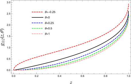
Figure 1: The variation of $g_{3/2}\left(z,\theta\right)$ via $z$ for different values of $\theta.$

We notice on (22) that $N_{0}^{D}$ would be complex for $1+2\theta<0$. This non-physical behavior imposes a strong condition on the Wigner parameter $\theta>-1/2$ which in turn means that the Dunkl formalism can only describe ideal Bose gases in these regimes. Considering this condition, we depict $g_{3/2}\left(z,\theta\right)$ versus $z$ via different Wigner parameters in Fig. 1. We observe that the function takes greater values when the Wigner parameter takes negative values, and smaller values when it takes positive values.

We also note that, in the limit of $\theta\rightarrow 0$, Eq. (26) reduces to the standard result:

$$\frac{N}{V}=\frac{N_{0}}{V}+\frac{g_{3/2}\left(z\right)}{\lambda^{3}}.$$ (28)

To our best knowledge, two methods exist to compute the condensation (or critical) temperature. The first method is to take $N_{0}^{D}=0$ in Eq. (26), and then, to work out $T_{c}^{D}$ [43, 44, 45, 46]. The second method is to calculate the temperature at which the specific heat of the system reaches its maximum value [47, 48]. In this manuscript, we use the fist method. We get

$$\frac{N}{V}=\frac{g_{3/2}(1)}{\lambda_{c}^{3}}\left[1+\frac{g_{3/2}(-1)}{g_{3/2}(1)}\left(1-\frac{1}{\sqrt{1+2\theta}}\right)\right],$$ (29)

where $N$ is the actual total particle number. Hence, the Dunkl-condensation temperature writes

$$\frac{T_{c}^{D}}{T_{c}^{0}}=\left[1+\frac{g_{3/2}(-1)}{g_{3/2}(1)}\left(1-\frac{1}{\sqrt{1+2\theta}}\right)\right]^{-2/3},$$ (30)

which clearly shows that the critical temperature is drastically modified by the Wigner parameter. Indeed, only in the limit $\theta\rightarrow 0$, do we obtain the standard condensation temperature $T_{c}^{0}=\frac{2\pi\hbar^{2}}{mk_{B}}\left(\frac{N}{Vg_{3/2}\left(1\right)}\right)^{2/3}.$ This effect is better visualized by plotting the temperature ratio versus the Wigner parameter (Fig. 2). We observe that the transition temperature is smaller than $T_{c}^{0}$ when $-1/2<\theta<0$. On the other hand, when $\theta$ takes on positive values, $T_{c}^{D}$ becomes greater than $T_{c}^{0}$.

Figure 2: Critical temperature ratio versus the Wigner parameter.

Finally, below the transition temperature, one may use Eqs. (26) and (29) to derive the ground state population $\frac{N_{0}^{D}}{N}$

$$\frac{N_{0}^{D}}{N}=1-\left(\frac{T}{T_{c}^{D}}\right)^{3/2},$$ (31)

In Fig. 3, we plot the ground state population $\frac{N_{0}^{D}}{N}$ as a function of $T/T_{c}^{0}$ for various $\theta$.

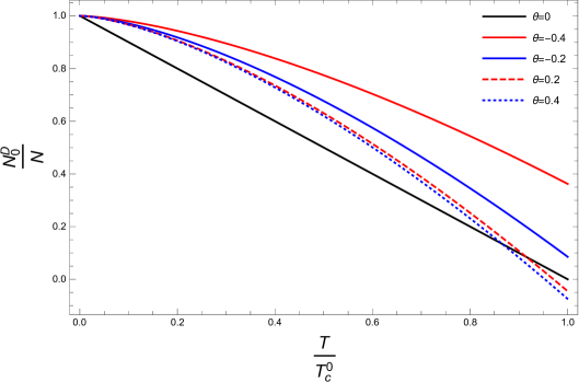
Figure 3: Ground state population vs. the temperature ratio $T/T_{c}^{0}$ for varying $\theta$.

4 Blackbody radiation

In this section, we examine the blackbody radiation phenomena within the Dunkl formalism. We start by expressing the mean occupation number of energy state of photons, $N_{\varepsilon}$, in the Dunkl formalism for the particular case of $\mu=0$.

$$N_{\varepsilon}=\frac{2}{e^{2\beta\varepsilon}z^{-2}-1}+\frac{(1+2\theta)}{e^{\beta(1+2\theta)\varepsilon}z^{-(1+2\theta)}+1}.$$ (32)

By assuming $\varepsilon=\hbar\omega$, where $\omega$ is the frequency of the photon, we write the number of photons within the frequency range of $\omega$ and $\omega+d\omega$ via:

$$dN_{\varepsilon}=\frac{V}{\pi^{2}c^{3}}\frac{\omega^{2}d\omega}{e^{2\beta\hbar\omega}-1}+\frac{V(1+2\theta)}{2\pi^{2}c^{3}}\frac{\omega^{2}d\omega}{e^{\beta(1+2\theta)\hbar\omega}+1}.$$ (33)

Hence, the corresponding energy density to this radiation reads:

$$\frac{dE^{D}}{V}=\frac{\hbar}{2\pi^{2}c^{3}}\left[\frac{2\omega^{3}}{e^{\frac{2\hbar\omega}{\mathbf{k}_{B}T}}-1}+\frac{(1+2\theta)\omega^{3}}{e^{\frac{(1+2\theta)\hbar\omega}{\mathbf{k}_{B}T}}+1}\right]d\omega.$$ (34)

After obtaining the generalized Planck radiation law in the framework of Dunkl-statistics we integrate it over all frequencies. We find the deformed total energy radiated by the cavity in the form of

$$\frac{E^{D}}{V}=\frac{\sigma}{2c}T^{4}\left[1+\frac{7}{\left(1+2\theta\right)^{3}}\right],$$ (35)

where $\sigma$ is the Stefan-Boltzmann constant. We observe that the Dunkl-correction to the standard energy radiation arises with the second term of Eq. (35). We note that for $\theta=0$ the Dunkl-corrected energy reduces to its conventional form, $\frac{E}{V}=\frac{4\sigma}{c}T^{4}$. In order to observe the effect of the Dunkl formalism, we depict the radiated Dunkl energy by the cavity, $\frac{E^{D}}{V}$, versus the temperature according to different deformation parameters in Fig. 4.

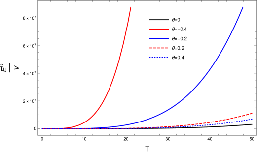
Figure 4: Dunkl-corrected energy radiation per unit volume versus the temperature for different values of $\theta$.

We see that the radiated energy increases with the increasing temperature as in the ordinary case. We also note that for a fixed value of temperature, the energy radiation decreases when the deformation parameter grows.

Next, we investigate several thermal quantities of the blackbody. First, we study Dunkl-corrected Helmholtz free energy by employing

$$F^{D}=-T\int\frac{E^{D}}{T^{2}}dT.$$ (36)

After we substitute Eq. (35) into Eq. (36), we arrive at,

$$\frac{F^{D}}{V}=-\frac{\sigma}{6c}T^{4}\left[1+\frac{7}{(1+2\theta)^{3}}\right].$$ (37)

In the limit of $\theta\rightarrow 0$, we get the ordinary case result, $F=-\frac{4V}{3c}\sigma T^{4}$. In Fig. 5, we demonstrate the Dunkl-Helmholtz free energy versus temperature.

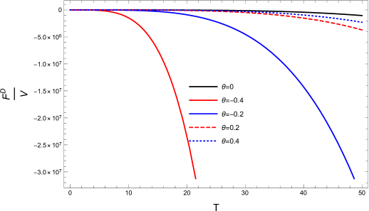
Figure 5: Dunkl Helmholtz free energy per unit volume versus temperature for different values of $\theta$.

We observe that in all cases the Dunkl-Helmholtz free energy decreases monotonically versus the increasing temperature. We also see that, for a fixed value of $T$, the free energy function increases when the deformation parameter $\theta$ grows.

The Dunkl-corrected entropy $S=-\left(\frac{\partial F}{\partial T}\right)$ is also of great interest. We indeed find the expression

$$\frac{S^{D}}{V}=\frac{2}{3c}\sigma T^{3}\left[1+\frac{7}{(1+2\theta)^{3}}\right],$$ (38)

which shows, upon gathering (37) and (35) that the thermodynamic functions satisfy the standard relation

$$F^{D}=E^{D}-TS^{D}.$$ (39)

The behavior of the Dunkl-corrected entropy versus temperature is depicted in Fig.

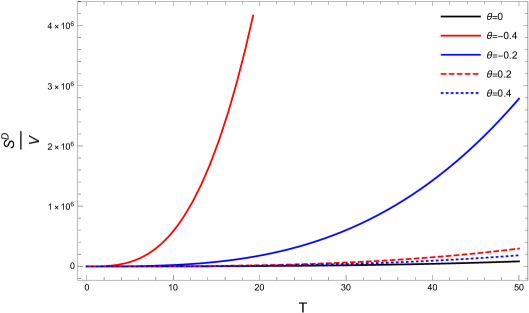
Figure 6: The Dunkl entropy per unit volume as a function of temperature for different values of $\theta$.

We see that at low temperatures the effect of Dunkl formalism is not observable. At high temperatures, this effect not only becomes significant but there is also a saturation point for $\theta$ growing to infinity, where one recovers the standard $T^{3}$ law with a different coefficient.

Next, we study the Dunkl-corrected specific heat function at constant volume, given by

$$C_{V}^{D}=-\left(\frac{\partial E^{D}}{\partial T}\right)_{V}=\frac{2V}{c}\sigma T^{4}\left[1+\frac{7}{(1+2\theta)^{3}}\right].$$ (40)

In the limit of $\theta\rightarrow 0$, Eq. (40) gives the standard result. We depict the behavior of the Dunkl-corrected specific heat versus temperature in Fig. 7.

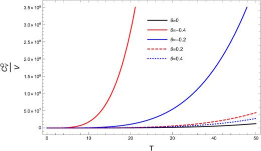
Figure 7: Dunkl specific heat per unit volume as a function of temperature for different values of $\theta$.

We notice that the deformed specific heat function increases with increasing temperature. This increase is greater for negative Wigner parameter.

Finally, we calculate the Dunkl-corrected pressure function of the model:

$$P=-\left(\frac{\partial F}{\partial V}\right)_{T}.$$ (41)

After substituting (37) into (41), we obtain

$$P^{D}=\frac{\sigma}{6c}T^{4}\left[1+\frac{7}{\left(1+2\theta\right)^{3}}\right].$$ (42)

This yields the equation of state (EOS) in the form

$$P^{D}V=\frac{E^{D}}{3},$$ (43)

which shows that the EOS is invariant within Dunkl formalism.

5 Conclusion

In this manuscript, we employed Dunkl formalism to investigate two important phenomena in physics. The ideal Bose gas in the grand canonical ensemble, where we construct the partition function and derive the total number of particles and the condensation temperature. A rigorous constraint appears on the Wigner parameter, namely $\theta>-1/2$. Moreover, we found that the deformed critical temperature becomes smaller or greater than the non-deformed one according to the negative and positive values of the deformation parameter.

In a second illustration, we examined the blackbody radiation within the Dunkl formalism. We derived the total energy radiated and studied various thermodynamic functions such as the Helmholtz free energy, the entropy, the specific heat, and the pressure of the system. We observed first that the Dunkl formalism leads to the same temperature dependence laws as the non-deformed case but with coefficients depending on the deformation parameter. These coefficients show a characteristic dependence on $\theta$. Finally, we noticed that the equation of state is invariant in the Dunkl formalism.

Finally, it’s worthwhile to mention that the occurrence of Bose-Einstein condensation in an ideal gas is an elementary illustration of a phase transition. A rigorous development of this phenomenon was given in Refs [53, 50, 51, 49, 52]. M. van den Berg et al. studied the Bose-Einstein condensation in the perfect boson gas due to the standard saturation mechanism in a prism of volume $V$ with sides $V^{\alpha}$, $V^{\gamma}$, $V^{\delta}$ with $\alpha\geq\gamma\geq\delta>0$ and $\alpha+\gamma+\delta=1$ in [53] and showed that:

$I$

: if $\alpha<1/2$, above the critical density $\rho_{c}$, the condensation is formed only in the ground states.

$II$

: if $\alpha=1/2$, the condensation is formed in an infinite number of single-particle states in a band with $\rho>\rho_{c}$.

$III$

: if $\alpha>1/2$, non-extensive occupation is formed where $\rho_{0}=\rho-\rho_{c}.$

Within the Dunkl formalism, the boson gas in rectangular parallelepiped of volume $V$ with sides of length $V^{\alpha}$, $V^{\gamma}$, $V^{\delta}$ may follow from a finite critical density the same way as in the conventional ideal Bose gas case. This case requires a thorough discussion which is currently under consideration and will be the subject of another study.

Data Availability Statements

The authors declare that the data supporting the findings of this study are available within the article.

References

- [1] E. P. Wigner, Phys. Rev. 77, 711 (1950).
- [2] L. M. Yang, Phys. Rev. 84, 788 (1951).
- [3] C. F. Dunkl, T. Am. Math. Soc. 311(1), 167 (1989).
- [4] M. Rösler, Lecture Notes in Mathematics 1817, 93 (Springer, Berlin) 2003.
- [5] L. Lapointe, L. Vinet, Commun. Math. Phys. 178(2), 425 (1996).
- [6] S. Kakei, J. Phys. A 29, L619 (1996).
- [7] S. M. Klishevich, M. S. Plyushchay, M. Rausch de Traubenberg, Nucl. Phys. B 616, 419 (2001).
- [8] P. A. Hortváthy, M. Plyushchay, M. Valenzuela, Ann. Phys. 325, 1931 (2010).
- [9] V. Genest, M. Ismail, L. Vinet, A. Zhedanov, J. Phys. A 46, 145201 (2013).
- [10] V. Genest, L. Vinet, A. Zhedanov, J. Phys. A 46, 325201 (2013).
- [11] V. Genest, M. Ismail, L. Vinet, A. Zhedanov, Commun. Math. Phys. 329, 999 (2014).
- [12] V. Genest, L. Vinet, A. Zhedanov, J. Phys. Conf. Ser. 512, 012010 (2014).
- [13] M. R. Ubriaco, Physica A 414, 128 (2014).
- [14] V. Genest, A. Lapointe, L. Vinet, Phys. Lett. A 379, 923 (2015).
- [15] E. J. Jan, S. Park, W. S. Chung, J. Kor. Phys. Soc. 68(3), 379 (2016).
- [16] M. Salazar-Ramirez, D. Ojeda-Guillén, V. D. Granados, Eur. Phys. J. Plus 132, 39 (2017).
- [17] M. Salazar-Ramirez, D. Ojeda-Guillén, R. D. Mota, V. D. Granados, Mod. Phys. Lett. A 33(20), 1850112 (2018).
- [18] S. Sargolzaeipor, H. Hassanabadi, W. S. Chung, Mod. Phys. Lett. A 33(25), 1850146 (2018).
- [19] W. S. Chung, H. Hassanabadi, Mod. Phys. Lett. A 34(24), 1950190 (2019).
- [20] S. Ghazouani, I. Sboui, M. A. Amdouni, M. B. El Hadj Rhouma, J. Phys. A: Math. Theor. 52, 225202 (2019).
- [21] R. D. Mota, D. Ojeda-Guillén, M. Salazar-Ramírez, V. D. Granados, Ann. Phys. 411, 167964 (2019).
- [22] W. S. Chung, H. Hassanabadi, Rev. Mex. Fis. 66(3), 308 (2020).
- [23] Y. Kim, W. S. Chung, H. Hassanabadi, Rev. Mex. Fis. 66(4), 411 (2020).
- [24] D. Ojeda-Guillén, R. D. Mota, M. Salazar-Ramírez, V. D. Granados, Mod. Phys. Lett. A 35(31), 2050255 (2020).
- [25] R. D. Mota, D. Ojeda-Guillén, M. Salazar-Ramírez, V. D. Granados, Mod. Phys. Lett. A 36(10), 2150066 (2021).
- [26] R. D. Mota, D. Ojeda-Guillén, M. Salazar-Ramírez, V. D. Granados, Mod. Phys. Lett. A 36(23), 2150171 (2021).
- [27] A. Merad, M. Merad, Few-Body Syst. 62, 98 (2021).
- [28] W. S. Chung, H. Hassanabadi, Mod. Phys. Lett. A 36(18), 2150127 (2021).
- [29] W. S. Chung, H. Hassanabadi, Eur. Phys. J. Plus. 136, 239 (2021).
- [30] H. Hassanabadi, M. de Montigny, W. S. Chung, Physica A 580, 126154 (2021).
- [31] S. H. Dong, W. H. Huang, W. S. Chung, P. Sedaghatnia, H. Hassanabadi, EPL 135, 30006 (2021).
- [32] B. Hamil, B. C. Lütfüoğlu, Few-Body Syst, 63, 74 (2022).
- [33] B. Hamil, B. C. Lütfüoğlu, Eur. Phys. J. Plus 137, 812 (2022).
- [34] P. Sedaghatnia, H. Hassanabadi, W. S. Chung, B. C. Lütfüoğlu, S. Hassanabadi, J. Kriz, arxiv:2208.12416 [quanth-ph].
- [35] R. D. Mota, D. Ojeda-Guillén, Mod. Phys. Lett. A 37(01), 2250006 (2022).
- [36] S. Hassanabadi, J. Kriz, B. C. Lütfüoğlu, H. Hassanabadi, Phys. Scr. 97, 125305 (2022).
- [37] N. Rouabhia, M. Merad, B. Hamil. Under review in EPL.
- [38] S. Hassanabadi, P. Sedaghatnia, W. S. Chung, B. C. Lütfüoğlu, J. Kriz, H. Hassanabadi, Eur. Phys. J. Plus 138, 331 (2023).
- [39] L. Vinet, A. Zhedanov, Rev. Math. Phys. 34(08), 2250025, (2022).
- [40] W. Greiner, L. Neise and H. Stocker, Thermodynamics and Statistical Mechanics (SpringerVerlag, New York, 1995).
- [41] A. Lavagno, P. Narayana Swamy, Phys. Rev. E 65, 036101 (2002).
- [42] E. H. Lieb, R. Seiringer, J. P/ Solovej, J. Yngvason, arXiv:cond-mat/0610117.
- [43] S. Grossmann, M. Holthaus, Phys. Lett. A 208, 188 (1995).
- [44] S. Grossmann, M. Holthaus, Z. Naturforsch. A 50, 921 (1995).
- [45] Q. -J. Zeng, Y. -S. Luo, Y. -G. Xu, H. Luo, Physica A 398, 116 (2014).
- [46] Q. -J. Zeng, Z. Cheng, J. -H. Yuan, Physica A 391, 563 (2012).
- [47] K. Kirsten, D. J. Toms, Phys. Rev. A 54, 4188 (1996).
- [48] K. Kirsten, D. J. Toms, Phys. Lett. A 222, 148 (1996).
- [49] F. Rocca, M. Sirugue, D. Testard, Commun. Math. Phys. 19, 119 (1970).
- [50] J. T. Lewis, J. V. Pule, Commun. Math. Phys. 36, 1 (1974).
- [51] D. W. Robinson, Commun. Math. Phys. 50, 53 (1976).
- [52] L. J. Landau, I. F. Wilde, Commun. Math. Phys. 70, 43 (1979).
- [53] M. van den Berg, J. T. Lewis, Physica A 110, 550 (1982).