Hadronic structure on the light-front VI.
Generalized parton distributions of unpolarized hadrons

Abstract

We discuss the generalized parton distributions (GPDs) for unpolarized hadrons, as a continuation of our recent work on hadronic structure on the light front. We analyze the unpolarized GPDs for the light nucleon and delta, as well as generic mesons, using the lowest Fock states. We use these GPDs to reconstruct the charge and gravitational form factors, and discuss their relative sizes. The results are also compared to reported QCD lattice results.

I Introduction

Light cone distributions are central to the description of hard inclusive and exclusive processes. Thanks to factorization, a hard process factors into a perturbatively calculable contribution times pertinent parton distribution and fragmentation functions. Standard examples can be found in deep inelastic scattering, Drell-Yan process and jet production to cite a few.

The parton distribution functions (PDF) are forward matrix elements of the leading twist operators of pertinent light front wave functions. They are valued time-like and as such not readily amenable to lattice simulations. As a result, only few moments of the PDF have been accessible to numerical simulations. To overcome this difficulty, space-like quasi-parton distrribution functions (qPDF) for fixed hadron momentum have been suggested by Ji Ji (2013), which are perturbatively matched to the light front PDF in the large momentum limit.

The generalized parton distributions (GPD) are off-forward matrix elements of the leading quark and gluon operators on the light front. They capture more aspects of the partonic content of the light front wavefunctions. They provide a more comprehensive description of the partons in a hadron on the light front, that range from its longitudinal momentum distribution (PDF), to its spatial charge and current distributions as captured by form factors (FF). GPDs are accessible by semi-inclusive processes through deeply virtual Compton scattering (DVCS), and deeply virtual meson production Ji (1997a); Radyushkin (1997). DVCS has been pursued by the CLAS collaboration at JLab and the COMPASS collaboration at CERN, with more planned experiments at the future electron ion colliders (EIC, EIcC) Abdul Khalek et al. (2022); Anderle et al. (2021).

Throughout, we will only discuss the GPDs in the DGLAP or large-x region $\xi\leq x\leq 1$, with $x$ the parton fraction of the struck quark, and $\xi$ its longitudinal skewness, i.e. the fraction of light cone momentum transfer to the nucleon, with the total 4-momentum transfer $\Delta$ and $\Delta^{2}=t<0$ Belitsky and Radyushkin (2005) (and references therein). This regime corresponds to the quark bag diagram in DIS kinematics. The GPDs in the ERBL or low-x region $0\leq x\leq\xi$ are not accessible with our LF wavefunctions. This regime corresponds to a particle changing diagram, with different in-out Fock states. Because of this kinematical limitation, the important concept of Polynomiality cannot be checked from our results. In the forward limit with $\xi=0$ and $\Delta=0$, the GDPs reduce to pertinent PDFs, and integrate along $x$ to form factors irrespective of $\xi$, bringing together the concepts of parton densities and form factors.

The outline of this paper is as follows. In section II we recall the leading twist-2 definitions of the unpolarized and polarized GPDs for generic mesons, and summarize the pertinent kinematics. We also make explicit the unpolarized GPDs for the light and heavy mesons, using the generic form of the LF wavefunctions established in our earlier work . construct the leading and unpolarized GPD. In esction III we also detail the unpolarized and polarized GPDs for generic and non-exotic baryons, with their relevant kinematics. We carry the numerical analysis of the unpolarized GPD for the nucleon and $\Delta$-isobar, using the LF wavefunctions in Shuryak and Zahed (2021a, b). We show that the nucleon shape at various parton-x scans on the light front, is substantially different from the rest frame, especially for large-x. In section IV we show that the electromagnetic Dirac form factor of both the nucleon and $\Delta$-isobar, are recovered from the GPD for zero skewness. We make explicit the A-gravitational formfactor, with a comparison to the Dirac formfactor. The results are also compared to available QCD lattice results. Our conclusions are in section V.

II Twist-2 GPDs of mesons

The GPDs provide a complete description of the leading twist-2 quark and gluon substructure in QCD of a hadron. They interpolate between the partonic densities and hadronic form factors, and as such provide a richer access to the hadronic structure Belitsky and Radyushkin (2005) (and references therein). More specifically, the GPDs are the twist-2 spin-j matrix elements of local quark- and gluon-operators, measured using LFWFs. At the resolution of about $\mu_{0}=1$ GeV, the LFWFs are composed of constituent quarks, with the non-perturbative gluons giving rise to the constituent masses, string tension and non-perturbative spin forces.

With this in mind, the leading and unpolarized GPD as a matrix element of solely the quark twist-2 spin-2 local operator, in a generic meson state on the LF, is Belitsky and Radyushkin (2005)

$${H}(x,\xi,t)=\int\frac{dz^{-}}{4\pi}e^{i\frac{x}{2}P^{+}z^{-}}$$

$$\times\langle M(p_{+})|\bar{q}(0)\gamma^{+}[0,z^{-}]q(z^{-})|M(p_{-})\rangle$$ (1)

with $z^{-}$ a time-like separation, for fixed $z^{+}=z_{\perp}=0$. The leading and polarized twist-2 meson GPD is defined as Belitsky and Radyushkin (2005)

$$\frac{iq_{\perp}^{i}\epsilon_{\perp}^{ij}}{2m_{M}}{E}(x,\xi,t)=\int\frac{dz^{-}}{4\pi}e^{i\frac{x}{2}P^{+}z^{-}}$$

$$\times\langle M(p_{+})|\bar{q}(0)i\sigma^{j+}\gamma^{5}[0,z^{-}]q(z^{-})|M(p_{-})\rangle$$ (2)

with $\epsilon_{\perp}^{ij}$ the antisymmetric tensor in the transverse plane with $i,j=1,2$, and $\sigma^{j+}=\frac{i}{2}[\gamma^{j},\gamma^{+}]$. $H$ is chirally even and $E$ is chirally odd. The latter probes the spatial distribution of a transversely polarized quark in the boosted meson state. The GPD kinematics in the symmetric frame, is fixed as follows

$$p_{\pm}=P\pm\Delta/2,\qquad P=(P^{0},0_{\perp},P^{z}),$$

$$P\cdot\Delta=0,\qquad t=-\Delta^{2},\qquad P^{2}=-m_{M}^{2}+\frac{1}{4}t,$$

$$x=\frac{k^{+}}{P^{+}},\qquad\xi=\frac{p_{+}^{+}-p_{-}^{+}}{p^{+}_{+}+p_{-}^{+}}=-\frac{\Delta^{+}}{2P^{+}}\,.$$ (3)

Note that we use the mostly-plus metric convention, so on-shell squared momenta are negative, and $t<0$. The light-front longitudinal skewness is referred to as $\xi$. The Wilson link will be set as $[0,z^{-}]\rightarrow 1$ throughout.

II.1 Mesons

Any meson is characterized by three leading Fock state wavefunctions, that mix under $L_{z},S_{z}$ on the LF. The classification of the states is done using $\Lambda=(S_{1}+S_{2})_{z}+L_{z}$, so the labelling $\Lambda=0,\pm 1$. Although $\Lambda=\pm 1$ are tied by symmetry modulo a trivial azimuthal phase, we will keep the three-label assignment. For the net $\Lambda=0$ meson pseudoscalar ($P$) and vector ($V$) states we have Ji et al. (2004)

$$|P\rangle = \int d[1]d[2]{\delta_{ij}\over\sqrt{N_{c}}}\ \big{[}\psi_{0}^{P}(x,k_{\perp})\big{(}Q_{i\uparrow}^{\dagger}(1)\bar{Q}_{j\downarrow}^{\dagger}(2)-Q_{i\downarrow}^{\dagger}(1)\bar{Q}_{j\uparrow}^{\dagger}(2)\big{)}$$ (4)

$$\qquad\qquad\qquad+\psi_{-1}^{P}(x,\vec{k}_{\perp})Q_{i\uparrow}^{\dagger}(1)\bar{Q}_{j\uparrow}^{\dagger}(2)+\psi_{+1}^{P}(x,\vec{k}_{\perp})Q_{i\downarrow}^{\dagger}(1)\bar{Q}_{j\downarrow}^{\dagger}(2)\big{]}|0\rangle$$

$$|V\rangle = \int d[1]d[2]{\delta_{ij}\over\sqrt{N_{c}}}\ \big{[}\psi_{0}^{V}(x,k_{\perp})\big{(}Q_{i\uparrow}^{\dagger}(1)\bar{Q}_{j\downarrow}^{\dagger}(2)+Q_{i\downarrow}^{\dagger}(1)\bar{Q}_{j\uparrow}^{\dagger}(2)\big{)}$$ (5)

$$\qquad\qquad\qquad+\psi_{-1}^{V}(x,\vec{k}_{\perp})Q_{i\uparrow}^{\dagger}(1)\bar{Q}_{j\uparrow}^{\dagger}(2)-\psi_{+1}^{V}(x,\vec{k}_{\perp})Q_{i\downarrow}^{\dagger}(1)\bar{Q}_{j\downarrow}^{\dagger}(2)\big{]}|0\rangle$$

with $N_{c}=3$, for the pseudoscalar and vector respectively. The subscripts $0$ and $\pm 1$ on the wave-functions, refer to $L_{z}$, the z-projections of the orbital momentum. Note that compared to the notations in Ji et al. (2004), there are no explicit factors of $k_{\perp}^{\pm}=k_{1}\pm ik_{2}$ here because they naturally belong to our wave functions, consistently defined not only for $m=L_{z}=1$, but for any $m$ value. Inserting (4) into (II-II) and carrying the contractions yields for the pseudoscalar P-state and unpolarized GPD, at zero skewness

$$H(x,0,t)=\sum_{\Lambda=0,\pm 1}\int\frac{dk_{\perp}}{(2\pi)^{3}}\psi_{\Lambda}^{P*}(x,k_{\perp}^{\prime})\psi_{\Lambda}^{P}(x,k_{\perp})$$

while for the polarized P-state and zero skewness ($j=1,2$)

$$\frac{i\Delta^{j}_{\perp}}{2m_{M}}E(x,0,t)=\int\frac{dk_{\perp}}{(2\pi)^{3}}$$

$$\bigg{(}(-i)^{j}\bigg{(}\psi^{P*}_{-1}(x,k_{\perp}^{\prime})\psi^{P}_{0}(x,k_{\perp})+\psi^{P*}_{0}(x,k^{\prime}_{\perp})\psi^{P}_{+1}(x,k_{\perp})\bigg{)}+(+i)^{j}\bigg{(}\psi^{P*}_{+1}(x,k^{\prime}_{\perp})\psi^{P}_{0}(x,k_{\perp})+\psi^{P*}_{0}(x,k_{\perp}^{\prime})\psi^{P}_{-1}(x,k_{\perp})\bigg{)}\bigg{)}$$

The kinematical arrangement is as follows: a/ active quark: $k_{\perp}^{\prime}=k_{\perp}+(1-x)\Delta_{\perp}$; b/ passive quark: $k_{\perp}^{\prime}=k_{\perp}-x\Delta_{\perp}$. The transferred momentum to the meson state is $t=-\Delta_{\perp}^{2}$.

More specifically, we will assume that the struck quark is the one with momentum fraction $x$, and that the kick momentum $\vec{\Delta}_{\perp}$ is in transverse 1-direction. Then after the kick, the the longitudinal and transverse momenta in the 1-direction (in primed notations) are

$$x_{1}^{\prime}={x-\xi\over 1-\xi},\,\,\,x_{2}^{\prime}=1-x$$

$$k_{1}^{\prime}=k+\Delta_{\perp}{1-x\over 1-\xi},\,\,k_{2}^{\prime}=k-\Delta_{\perp}{x\over 1-\xi}$$ (8)

Our detailed analyses in Shuryak and Zahed (2021a, b) show that the mesonic LF wavefunctions can be well approximated by a Gaussian $\psi(k,x)\sim e^{-A(x)(k_{1}^{2}+k_{2}^{2})}$, where $A(x)$ depends on the specific nature of the meson. As a result, the meson LF wavefunction after the kick $\psi(k^{\prime},x^{\prime})$ follows through the substitution $(k_{1}^{2}+k_{2}^{2})\rightarrow(k_{1}^{\prime 2}+k_{2}^{\prime 2})$. Using (II.1) to calculate the unpolarized GPD $H(x,0,-\Delta_{\perp}^{2})$ at zero skewness, yields

$$H(x,0,-\Delta_{\perp}^{2})\sim e^{-A(x)\big{(}3/4-x(1-x)\big{)}\Delta_{\perp}^{2}}$$ (9)

III Twist-2 spin-2 GPDs of the nucleon

The leading nucleon GPDs are also driven by the leading twist-2 and spin-2 vector and axial-vector currents on the light front. As we noted earlier for the mesons, our construction of the nucleon LFWFs restricts our analysis of the GPDs to the DGLAP region, with particle preserving in-out Fock states. Also at the resolution of $\mu_{0}=1$ GeV, the nucleon is limited to the lowest 3-quark Fock state, where the GPDs are limited to their constituent quark content. In this section, we will quote the general results for the unpolarized and polarised GPDs for generic baryons. The unpolarized GPD for the nucleon and $\Delta$-isobar will be made more explicit using our LFWFs in Shuryak and Zahed (2022a, b).

III.1 General expressions and kinematics

The quark GPDs of the nucleon are captured by the off-diagonal formfactors Belitsky and Radyushkin (2005)

$$\int\frac{P^{+}dz^{-}}{4\pi}e^{\frac{1}{2}ixz^{-}P^{+}}\langle p_{+}\Lambda_{+}|\overline{q}(0)\gamma^{+}[0,z^{-}]q(z^{-})|p_{-}\Lambda_{-}\rangle=$$

$$\overline{N}(p_{+},\Lambda_{+})\bigg{(}H(x,\xi,t)\gamma^{+}+E(x,\xi,t)\frac{i\sigma^{+j}\Delta_{j}}{2m_{N}}\bigg{)}N(p_{-},\Lambda_{-})$$

$$\int\frac{P^{+}dz^{-}}{4\pi}e^{\frac{1}{2}ixz^{-}P^{+}}\langle p_{+}\Lambda_{+}|\overline{q}(0)\gamma^{+}\gamma_{5}[0,z^{-}]q(z^{-})|p_{-}\Lambda_{-}\rangle=$$

$$\overline{N}(p_{+},\Lambda_{+})\bigg{(}\tilde{H}(x,\xi,t)\gamma^{+}\gamma_{5}+\tilde{E}(x,\xi,t)\frac{\Delta^{+}\gamma_{5}}{2m_{N}}\bigg{)}N(p_{-},\Lambda_{-})$$ (10)

Here $H,E$ are the unpolarized quark GPDs, and $\tilde{H},\tilde{E}$ their polarized counterparts. Note that for $\xi=0$, we have $t=-\Delta_{\perp}^{2}$, and $\tilde{E}$ drops out. The generic form of the nucleon wavefunction is

$$|p\Lambda\rangle=\int\prod_{i=1}^{3}\frac{dx_{i}dk_{i\perp}}{\sqrt{x_{i}}}\delta\bigg{(}1-\sum_{i=1}^{3}x_{i}\bigg{)}\,\delta\bigg{(}\sum_{i=1}^{3}k_{i\perp}\bigg{)}\psi^{\Lambda}([x_{i},k_{i\perp},\lambda_{i}])|[x_{i}p^{+},k_{i\lambda}+x_{i}p_{i\perp},\lambda_{i}]\rangle$$ (11)

for a nucleon of total momentum $p^{\mu}$ and helicity $\Lambda=\pm 1$. The conversion to the Jacobi coordinates is subsumed, with the delta-functions readily enforced. At low resolution, the nucleon state $\psi^{\Lambda}$ is a quark-diquark $q[qq]_{0}$ Fock state.

To proceed, we note the identities for the matrix elements of the nucleon spinors in (III.1) on the right-hand-side,

$$\overline{N}(p_{+},\Lambda_{+})\gamma^{+}N(p_{-}\Lambda_{-}) = 2P^{+}\frac{\sqrt{1-\xi}}{1-\frac{1}{2}\xi}\,\delta_{\Lambda_{+}\Lambda_{-}}$$

$$\overline{N}(p_{+},\Lambda_{+})\frac{i\sigma^{+j}\Delta_{j}}{2m_{N}}N(p_{-}\Lambda_{-}) = 2P^{+}\bigg{(}-\frac{1}{4}\frac{\xi^{2}}{(1-\frac{1}{2}\xi)\sqrt{1-\xi}}\delta_{\Lambda_{+}\Lambda_{-}}+\frac{\Lambda_{-}q^{1}+iq^{2}}{2m_{N}}\frac{1}{\sqrt{1-\xi}}\delta_{(-\Lambda_{+})\Lambda_{-}}\bigg{)}$$ (12)

Inserting the free field decomposition of the good component of the quark field in (III.1), and carrying the contractions yield the respective GPDs.

Zero skewness:

$$H(x,0,t) = \int_{P}\delta(x-x_{1})\,\psi^{+*}([x^{\prime}_{i},k^{\prime}_{i\perp},\lambda_{i}])\psi^{+}([x_{i},k_{i\perp},\lambda_{i}])$$

$$E(x,0,t) = \frac{-2m_{N}}{q_{L}}\int_{P}\delta(x-x_{1})\,\psi^{+*}([x^{\prime}_{i},k^{\prime}_{i\perp},\lambda_{i}])\psi^{-}([x_{i},k_{i\perp},\lambda_{i}])$$

$$\tilde{H}(x,0,t) = \int_{P}\lambda_{1}\,\delta(x-x_{1})\,\psi^{+*}([x^{\prime}_{i},k^{\prime}_{i\perp},\lambda_{i}])\psi^{+}([x_{i},k_{i\perp},\lambda_{i}])$$

with $q_{L}=q^{1}-iq^{2}$, and the phase space helicity sum and integration

$$\int_{P}=\sum_{[\lambda_{i}]}\int\prod_{i=1}^{3}dx_{i}d^{2}k_{i\perp}\,\delta\bigg{(}1-\sum_{i=1}^{3}x_{i}\bigg{)}\,\delta\bigg{(}\sum_{i=1}^{3}k_{i\perp}\bigg{)}$$ (14)

The kinematical arrangement is as follows: a/ active quark $i=1$: $x_{1}^{\prime}=x_{1}$ and $k_{1\perp}^{\prime}=k_{1\perp}+(1-x_{1})\Delta_{\perp}$ and $\lambda_{1}=\pm 1$; b/ passive quarks $i=2,3$: and $x_{i}^{\prime}=x_{i}$ and $k_{i\perp}^{\prime}=k_{1\perp}-x_{i}\Delta_{\perp}$.

Finite skewness:

$$\frac{\sqrt{1-\xi}}{1-\frac{1}{2}\xi}H(x,\xi,t)-\frac{1}{4}\frac{\xi^{2}}{(1-\frac{1}{2}\xi)\sqrt{1-\xi}}E(x,\xi,t)=\int_{P}\delta(x-x_{1})\,\psi^{+*}([x^{\prime}_{i},k^{\prime}_{i\perp},\lambda_{i}])\psi^{+}([x_{i},k_{i\perp},\lambda_{i}])$$ (15)

and

$$-\frac{q_{L}}{2m_{N}}\frac{1}{\sqrt{1-\xi}}E(x,\xi,t)=\int_{P}\delta(x-x_{1})\,\psi^{+*}([x^{\prime}_{i},k^{\prime}_{i\perp},\lambda_{i}])\psi^{-}([x_{i},k_{i\perp},\lambda_{i}])$$ (16)

The kinematical arrangement is as follows: a/ active quark $i=1$: $x_{1}^{\prime}=(x_{1}-\xi)/(1-\xi)$ and $k_{1\perp}^{\prime}=k_{1\perp}+((1-x_{1})/(1-\xi))\Delta_{\perp}$ and $\lambda_{1}=\pm 1$; b/ passive quarks $i=2,3$: and $x_{i}^{\prime}=x_{i}$ and $k_{i\perp}^{\prime}=k_{1\perp}-(x_{i}/(1-\xi))\Delta_{\perp}$.

III.2 $N,\Delta$ GPDs from the LFWFs with $\xi=0$

The unpolarized GPDs for the nucleon and $\Delta$-isobar can be explicitly evaluated using the the explicit LFWFs developed in Shuryak and Zahed (2022b), to which we refer for most of the details. Here, we briefly recall for the flavor and spin symmetric isobar $\Delta^{++}=uuu$, the LF Hamiltonian is the sum of the kinetic energies of three u-constituents, plus their confining potentials (the hyperfine spin forces are smal and can be added in perturbation). The proton $uud$ is composed of a flavor-spin asymmetric $[ud]$ diquark paired by the instanton-induced ^′t Hooft interaction, treated in the quasi-local approximation. This diquark pairing is responsible for the mass splitting between the nucleon and the $\Delta$-isobar, and the difference between thei respective LFWFs.

For the proton with quark assignment $uud$, we assume that the struck quark is $d$, with longitudinal momentum fraction $x_{3}$. In our (modified) Jacobi coordinates, this momentum fraction is directly related to the longitudinal variable $\lambda$. For the unpolarized d-quark GPD in (15), this amounts to integrating the off-forward LFWFs over 5 variables, the transverse momenta $\vec{p}_{\rho},\vec{p}_{\lambda}$ and $\rho$ for the nucleon. To proceed, we approximate the dependence on the transverse momenta $\vec{p}_{\rho},\vec{p}_{\lambda}$ by Gaussians, which is quite accurate, and carry the integrals analytically. The remaining integration over $\rho$ is performed numerically. We recall that the LFWFs are generated at a low renormalization scale, say $\mu_{0}=1$ GeV, with a nucleon composed of three constituent quarks, without constituent gluons. (The nonperturbative vacuum gluonic fields and hard gluons are all repackaged in the constituent quark mass and chiral condensate on the LF).

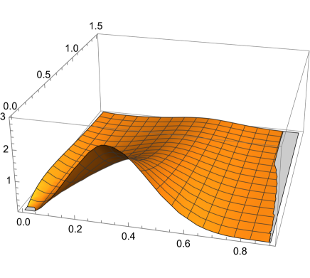
Figure 1: The nucleon GPD function $H_{d}^{N}(x,\xi=0,Q^{2})$ for a struck d-quark.

In Fig.1 we show the unpolarized nucleon GPD for the struck d-quark, as a function of $x,Q^{2}$ and zero skewness. At small $Q^{2}$, the dependence on the longitunal parton momentum $x$, is that expected for a PDF with a maximum at $x=\frac{1}{3}$. At larger $Q^{2}$, the maximum of the GPD clearly shifts towards larger values of $x$. The GDP is not simply factorizable into the PDF times the form factor, which are separable in $x$ and $Q^{2}$. The right shift in Fig.1 shows that the nucleon shape changes with $x$. This is a key point of interest to us, as we now proceed to detail these shape modifications.

Theoretical considerations Guidal et al. (2005) have suggested that the GPDs can be approximated generically, by a “Gaussian ansatz" in the momentum transfer $Q^{2}$, with a width and a pre-exponent that are x-dependent

$${\rm GPDs}(x,Q^{2})\sim f_{1}(x)\,e^{-Q^{2}f_{2}(x)}$$ (17)

We recall that the standard nucleon formfactors are dipole-like at low $Q^{2}$ (say lower than 10 GeV²) with $F(Q^{2})\sim 1/(m^{2}+Q^{2})^{2}$. At very large $Q^{2}$ it asymptotes to a constant $Q^{4}F(Q^{2})\rightarrow const$ which is fixed by the perturbative QCD scattering rule. In between, the $Q^{2}$ dependence remains an open issue.

Our LF formfactors were found to be consistent with these observations (see below), and our GPDs at fixed $x$ are indeed numerically consistent with the exponent

$$e^{-\frac{Q^{2}f_{s}(x)}{\sqrt{1-\xi^{2}}}}$$ (18)

with no dependence of the pre-expont on the skewness, for $x>\xi$. We have checked that the x-integration of this exponent with $\xi=0$, returns the expected rational formfactor.

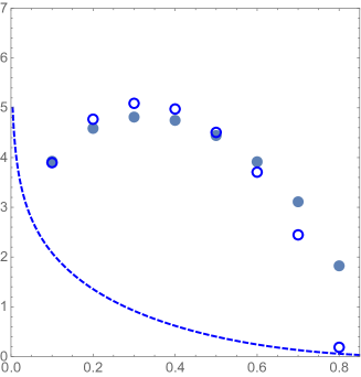
Figure 2: Closed and open points correspond to slopes $-dlog[{\rm GPD}]/dQ^{2}$ (at $Q^{2}\approx 1\,{\rm GeV}^{2}$) calculated from our LFWF for the nucleon and Delta baryons, respectively. The dashed line shown for comparison is the ansatz (20) .

The GPDs calculated from our LFWFs is well described by (17). In particular, the r.m.s. spatial size of the struck d-quark for fixed $x$ is

$$R_{r.m.s.}(x)=\sqrt{2f_{2}(x)}$$ (19)

In Fig.2 we show the effective Q-slope of the unpolarized d-quark GPD, for the nucleon (filled-points) and $\Delta$-isobar (open-points). The r.m.s. size $R_{r.m.s.}(x)$ is maximal at $x\sim\frac{1}{3}$, and is numerically about $0.6$ fm. It decreases sharply for $x\sim 1$, and moderatly for $x\sim 0$. This can be explained by the fact that for $x\sim\frac{1}{3}$, all three quarks carry about the same longitudinal momentum on the LH, which corresponds to three quarks at rest in the CM or rest frame. Semiclassically, this means a configuration in which a struck quark is near a “turning points" of the wave function, with their QCD strings maximally streched. In contrast, $x$ away from $\frac{1}{3}$, corresponds to a struck quark rapidly moving in the CM frame, which must happen near the hadron center, The corresponding size is therefore small. Note that for $x\rightarrow 1$, the distribution of the struck d-quark becomes nearly pointlike, with slopes close to zero. Our LFWFs show that the magnitude of this effect is different for nucleon and $\Delta$-isobar, sensitive to the the diquark substructure of the former.

The behavior of the GPDs near the edges $x\sim 0,1$, can be gleaned from general QCD considerations. The small x-region of the GPD is dominated by Regge physics Guidal et al. (2005), while the large x-region of the GDP is fixed by the Drell-Yan-West relation. A particular functional form for the GPD that abides by these two limits, was suggested in de Teramond et al. (2018)

$$H(x,0,t) \sim e^{tf(x)}$$ (20)

with $t=-Q^{2}$, and

$$f(x)={1\over 4\lambda}\bigg{(}(1-x)\,{\rm ln}\bigg{(}{1\over x}\bigg{)}+a(1-x)^{2}\bigg{)}$$

with the parameters $a=.53$ and $\lambda=(0.548\,{\rm GeV})^{2}$. In Fig.2 we show (20) (dashed-line) for comparison. The sharp rise at small $x$ is due to the parametrized Reggeon in (20), a multi-parton cloud around a baryon. It is absent in our approach, which is limited to the lowest Fock state. The decrease at large $x$ is in qualitative agreement with our results. However, at intermediate $x$ there is a significant disagreement, with our baryon r.m.s. size $R_{r.m.s.}(x)$, which is significantly larger.

IV Electromagnetic and gravitational form factors

On the LF the GPDs are related to various form factors of the nucleon. In particular, the n-Mellin moments of the GDP is a polynomial of degree $\xi^{n}$, a property known as polynomiality Belitsky and Radyushkin (2005). However, since the Mellin moments sum over both the ERBL region ($0<x<\xi$) and the DGLAP region ($\xi<x<1$), the polynomiality cannot be checked, as the ERBL region falls outside the scope of our analysis.

IV.1 Electromagnetic formfactors

This notwithstanding, a number of electromagnetic and gravitational formfactors of the nucleon, can be extracted from the present GPDs, allowing also for estimates of the spin and mass sum rules. More specifically, the Dirac $F_{1}$, the Pauli $F_{2}$ electromagnetic formfactors and the axial formfactor $G_{A}$, are all tied to the zeroth moment of the GPDs on the LF, at zero skewness Belitsky and Radyushkin (2005) (and references therein)

$$F_{1}(t) = \int dxH(x,0,t)$$

$$F_{2}(t) = \int dxE(x,0,t)$$

$$G_{A}(t) = \int dx\tilde{H}(x,0,t)$$ (21)

In Fig.3 we show the numerical results for $Q^{4}F^{d}_{1}$ versus $Q^{2}$ in ${\rm GeV}^{2}$, for a struck d-quark, following from the integration of the unpolarized d-quark $H$ GPD, for the nucleon (filled-point) and $\Delta$-isobar (open-point). The standard dipole-form factor with the rho mass is depicted by the solid-curve, using $Q^{4}/(1+Q^{2}/m_{\rho}^{2})^{2}$ and $m_{\rho}=780$ MeV. The results follow the dipole curve below 1 GeV², and deviate substantially above, to asymptote a constant at much larger $Q^{2}$, as expected from the QCD counting rules for both nucleons. The rescaled formfactor for the isobar is found to fall faster than the nucleon at large $Q^{2}$, which indicates that the nucleon is more compact electromagnetically than the isobar, with a smaller electromagnetic radius.

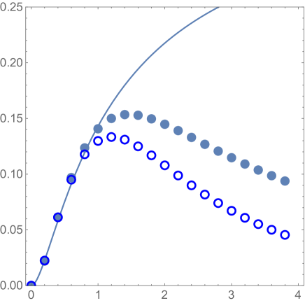
Figure 3: Scaled Dirac form factor $Q^{4}F_{1}^{d}(Q^{2})$ in GeV⁴ versus $Q^{2}$ in GeV², for the nucleon (filled-point) and $\Delta$ (open-point), obtained by integrating the unpolarized d-quark-H GDP. For comparison we show a “dipole fit" curve $Q^{4}/(1+Q^{2}/m_{\rho}^{2})^{2}$ (solid-line).

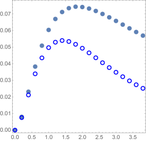
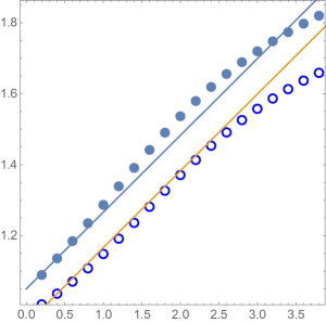
Figure 4: Scaled gravitational form factor $Q^{4}A_{d}(Q^{2})$ in GeV⁴ versus $Q^{2}$ in GeV² (top), for the struck d-quark in a nucleon (closed-points) and the isobar (open-points). Ratio of the gravitational to electromagnetic formfactors $3A^{d}(Q^{2})/F_{1}^{d}(Q^{2})$ versus $Q^{2}$ in GeV² (bottom), for the nucleon (closed-points) and the isobar (open points).

IV.2 Gravitational formfactors

As we noted earlier, our low-resolution LFWFs are dominated by the lowest Fock state of three constituent quarks. Hence, the GPD is mostly that of the constituent quarks. The first moment of the unpolarized GPDs at zero skewness, is tied to the quark $A,B$ form factors of the energy-momentum tensor Belitsky and Radyushkin (2005)

$$A(t) = \int dx\,xH(x,0,t)$$

$$B(t) = \int dx\,xE(x,0,t)$$ (22)

They can be used to quantify the distribution of momentum, angular momentum and pressure-like stress, inside the nucleon Polyakov and Schweitzer (2018) (and references therein). More specifically, the total nucleon angular momentum at this low-resolution, is given by Ji^′s sum rule Ji (1997b)

$$J=\frac{1}{2}=A(0)+B(0)$$ (23)

with the non-perturbative gluons implicit in the balance, as they enter implicitly in the composition of the LF Hamiltonian (mass, string tension, …) for the constituent quarks. Since our LFWFs are so far unpolarized, we do not have acces to the B-formfactor, as it involves the overlap between spin flipped LFWFs. The polarized GPDs together with the role of the spin forces, will be discussed elsewhere.

In Fig.4 (top) we show the numerical results for $Q^{4}A^{d}$ versus $Q^{2}$ in ${\rm GeV}^{2}$, for a struck d-quark, following from the integration of the unpolarized d-quark-A GPD, for the nucleon (filled-point) and $\Delta$-isobar (open-point). Again, we observe that the isobar form factor falls faster than the mucleon form factor, an indication that the nucleon is more compact gravitationally than the isobar, with a smaller gravitational radius. In Fig.4 (top) we plot the ratio of the gravitational formfactor relative to the electromagnetic form factor, for the struck d-quark in the nucleon (filled-points) and isobar (open-points). The decrease in $Q^{2}$ of the gravitational form factor, is slower than the electromagnetic form factor for both hadrons. This means that the spatial mass distribution of the struck d-quark, is more compact than the spatial charge distribution. More specifically, we find

$${3A_{d}(Q^{2})\over F^{d}_{1}(Q^{2})}=C_{0}+{Q^{2}\over M^{2}_{fit}},$$ (24)

with slopes close to one $C_{0}^{N}=1.05$, $C_{0}^{\Delta}=0.95$, $M_{fit}^{N}=M_{fit}^{\Delta}=2.15$ GeV. We have multiplied $A^{d}$ by a factor of 3, which accounts for the mean momentum $\langle x\rangle=1/3$, to bring the ratio close to 1.

IV.3 Comparison to lattice simulations

The moments of the GPDs at different momentum transfer $t$, were evaluated on the lattice. Here, we will follow the detailed analysis by the LHPC collaboration Hagler et al. (2008), where detailed numerical tables for the moments of the GPDs are given. More specifically, the longitudinal moments of the unpolarized nucleon GPD are defined as

$$H^{n}(\xi,t)=\int dxx^{n-1}H(x,\xi,t)$$ (25)

In their notations, the Dirac and gravitational formfactors at zero skewness $\xi=0$, are denoted by $A_{1}(0,t)$ and $A_{2}(0,t)$ respectively. Before we start comparing their results to ours, several warnings are in order.
(1) Although the simulations are done with domain wall fermions, they are still done with large quark masses. The pion mass varies between $m_{\pi}=760$ and $350\,{\rm MeV}$ for different datasets. The chiral extrapolation to a small physical mass is clearly nonlinear, and produce significant uncertainties.
(2) All reported results are quoted at a normalization scale $\mu^{2}=4\,{\rm GeV}^{2}$, a standard value used for internal and external comparison. As we repeatedly emphasized in the previous papers of this set, our LF wave functions and GPDs should correpond to a much lower normalization point, and even with “chiral evolution" are only taken up to $\mu^{2}_{\chi}=1\,{\rm GeV}^{2}$. The difference between them is significant: if at $\mu_{\chi}$ there are no gluons and the quark fraction of momentum is 1, at $\mu^{2}=4\,{\rm GeV}^{2}$ it is about twice smaller, and comparable to the gluon momentum fraction. As the famous “spin crisis" shows, a similar observation holds for the spin fractions carried by the quarks and gluons.
(3) The lattice spacing $a$ strongly limits the value of the largest momentum transfer which can be used, to roughly $|t|<1.2\,{\rm GeV}^{2}$. As one can see from our previous plots, interesting deviations from simple dipole fits only are visible at larger values.

With these issues in mind, we now address the main qualitative findings. Perhaps the most important observation is that the Dirac formfactor $A_{1}(0,t)$ decreases faster with $|t|$, than the gravitational formfactor $A_{2}(0,t)$. This implies that spatial distribution of quarks in the nucleon is wider than that of the stress tensor. While this qualitative phenomenon is by now established empirically Duran et al. (2022), the lattice data Hagler et al. (2008) quantify it. In Fig.5 we compare $t$-dependence for the ratio $A_{2}(0,|t|)/A_{1}(0,|t|)$, for our isoscalar $u+d$ nucleon GPD (filled points), with the lattice dataset 1 from Hagler et al. (2008) (open points).

The main take from this comparison is that the ratio grows with the momentum transfer, and the growth slope is similar for both results. However, the values of the ratio itself are not the same. This is expected, since the evolution of our results (filled points) to higher chiral scale $\mu^{2}_{\chi}=1\,{\rm GeV}^{2}$ should cause the quark PDFs to shift to smaller $x$, therefore lowering down our curve towards the reported lattice data points (open points).

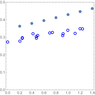
Figure 5: The ratio $A_{2}(0,|t|)/A_{1}(0,|t|)$ as a function of $|t|\,(GeV^{2})$ for our isoscalar $u+d$ nucleon GPD (filled points), and the lattice dataset 1 (open points) from Hagler et al. (2008).

A more recent lattice study in Bhattacharya et al. (2022), extracts the full GPDs from quasi-GPDs using the lattice momentum effective theory (LaMET) Ji (2013); Ji et al. (2021). Their result for the unpolarized nucleon GPD $H(x,\xi,t)$ with symmetric momentum assignment (their Fig. 18), is shown in Fig. 6 (black-solid line), for zero skewness $\xi=0$ and fixed $t=-0.69\,{\rm GeV}^{2}$. Note that we have only show the quark part of the lattice GPD, and only for $x>0.05$ (the validity of LaMET may even require a larger lower bound, say $x>0.1$ for current lattice nucleon momentum, see discussion in Ji et al. (2021)). Note also that the reported lattice data were evolved to the standard normalization scale $\mu^{2}=4\,GeV^{2}$.

Our current baryonic LFWFs are limited tho the 3-quark sector, and therefore to a low normalization point, where there are no gluons and $\bar{q}q$ sea. As explained in our previous works, after “chiral evolution" we used, the ensuing DAs, PDFs, GPDs can be evolved to the chiral normalization scale $\mu_{\chi}^{2}=1\,GeV^{2}$, and then by DGLAP, to any higher scales, such as $\mu^{2}=4\,{\rm GeV}^{2}$. We have not carried out any of this in the present comparison. Our results are also shown in Fig. 6 for the unpolarized GPD $H(x,\xi=0,t=-0.69\,{\rm GeV}^{2})$ (black-dashed line). For comparison, we also show our GPD $H(x,\xi=0,t=0)$ (dashed-blue line), which is effectively the PDF. The agreement between the lattice GPD and our GPD for $x>0.4$ is quite reasonable, modulo all the reservations. This is nontrivial, as the underlying $t$ dependence is rather strong, as seen from comparison to the $t=0$ GPD curve.

Figure 6: We show the lattice baryonic GPD $H(x,\xi=0,t=-0.69\,{\rm GeV}^{2}$) versus $x$following from LaMET in Bhattacharya et al. (2022) (black-solid line), and our result (dashed-black line). Our result for the GPD $H(x,\xi=0,t=0)$ which is the PDF (dashed-blue line), is shown for comparison.

IV.4 Nucleon tomography

The Fourier transform of the H GPD in the transverse part of the momentum transfer $\Delta_{T}$ with $\Delta_{T}^{2}=-t$, yields to a map for the spatial distribution of the partons (mostly constituent quarks here), with a fixed longitudinal momentum $x$

$$q(x,\xi,b)=\int\frac{d\Delta_{\perp}}{(2\pi)^{2}}e^{-i\Delta_{\perp}\cdot b}H(x,\xi,t=-\Delta_{T}^{2})$$ (26)

For an estimate, we use the approximate form (18), to obtain

$$q(x,\xi,b)\sim\frac{\sqrt{1-\xi^{2}}}{f_{s}(x)}e^{-\frac{b^{2}\sqrt{1-\xi^{2}}}{4f_{s}(x)}}$$ (27)

in the DGLAP regime with $x>\xi$. This impact-parameter-like representation of the GDP in transverse space, provides a 1+2 tomographic description of the partons inside the nucleon. In general, (26-27) allows for the characterization of the x-dependence of the parton distribution in a hadron. At large $b$ it reflects on the chiral physics (pion cloud), while at very low-x it is sensitive to the diffusion of wee partons.

V Conclusions

The interest in GPDs stems from their characterization of the partonic substructure of hadrons, in terms of parton longitudinal momentum, transverse position and spin. They can be related to certain hard processes, allowing their possible extraction from experiment. As such, they are important tools for the understanding hadronic structures in QCD.

The present work is a modest attempt along these directions, to try to understand how the spatial distribution of a struck quark in a hadron, depends on its longitudinal momentum $x$. For that, we made use of some of the results for the LFWFs, we have developed recently Shuryak and Zahed (2022a, b). We recall that these LFWFs are not just some parameterizations: they diagonalize certain LF Hamiltonians of increasing complexity, subject to the strictures of non-perturbative lattice QCD at low resolution (instantons, P-vortices, …).

In its simplest form, our LF Hamiltonian consists of the kinetic and confining contributions for flavor-symmetric (the $\Delta$-isobar) LFWF, plus a diiquark pairing term between flavor-asymmetric (light $ud$) quarks for the nucleon. So, for the $\Delta$-isobar, the LFWF exhibits triangular symmetry in the longitudinal parton fractions, while for the nucleon this symmetry is broken by diquark pairing.

Remarkably, our calculated GPDS for both the nucleon and the $\Delta$-isobar, are found to be numerically well described by a proposed Gaussian ansatz (17), with $x,\xi$ dependent width. However, the width is substantially different from that reported by other model calculations.

The GPDs integrated over $x$ give rise to the electromagnetic and gravitational formfactors. We have used our GPDs with our LFWFs, to recover the electromagnetic fom factors from our earlier results Shuryak and Zahed (2022b). We also derived anew, the nucleon A-gravitational formfactor. While both the electromagnetic and gravitational form factors appear similar and dipole-like, their ratio shows differences, an indication that the charge and mass composition are spatially distinct.

The GPDs encapsulate a vast amount of dynamical information regarding the partonic substructure of hadrons, with fixed $x,\xi,t$ kinematics. However, it is usually challenging to tie the theoretical insights and results for the GDPs, such as the ones based on the LFWFs we have detailed, with their extraction from semi-inclusive data. DIS probes the GPDs at the boundary $x=\xi$ of the finite $x-\xi$-domain, and the convolution integrals of the empirical GPDs are limited to the $\xi>0$ region. The sum rules require integrating over the longitudinal momentum $x$ for fixed $\xi$, while the tomography is carried at $\xi=0$. To relate these separate kinematic regimes, requires the use of the GDP global analytical properties, and models constrained by these properties, as well as lattice physics, as we have pursued.

Acknowledgements

We thank the members of the QGT collaboration for triggering our motivation for this work. This work is supported by the Office of Science, U.S. Department of Energy under Contract No. DE-FG-88ER40388.

References

- Ji (2013) X. Ji, Phys. Rev. Lett. 110, 262002 (2013), arXiv:1305.1539 [hep-ph] .
- Ji (1997a) X.-D. Ji, Phys. Rev. D 55, 7114 (1997a), arXiv:hep-ph/9609381 .
- Radyushkin (1997) A. V. Radyushkin, Phys. Rev. D 56, 5524 (1997), arXiv:hep-ph/9704207 .
- Abdul Khalek et al. (2022) R. Abdul Khalek et al., Nucl. Phys. A 1026, 122447 (2022), arXiv:2103.05419 [physics.ins-det] .
- Anderle et al. (2021) D. P. Anderle et al., Front. Phys. (Beijing) 16, 64701 (2021), arXiv:2102.09222 [nucl-ex] .
- Belitsky and Radyushkin (2005) A. V. Belitsky and A. V. Radyushkin, Phys. Rept. 418, 1 (2005), arXiv:hep-ph/0504030 .
- Shuryak and Zahed (2021a) E. Shuryak and I. Zahed, (2021a), arXiv:2111.01775 [hep-ph] .
- Shuryak and Zahed (2021b) E. Shuryak and I. Zahed, (2021b), arXiv:2112.15586 [hep-ph] .
- Ji et al. (2004) X.-d. Ji, J.-P. Ma, and F. Yuan, Eur. Phys. J. C 33, 75 (2004), arXiv:hep-ph/0304107 .
- Shuryak and Zahed (2022a) E. Shuryak and I. Zahed, (2022a), arXiv:2202.00167 [hep-ph] .
- Shuryak and Zahed (2022b) E. Shuryak and I. Zahed, (2022b), arXiv:2208.04428 [hep-ph] .
- Guidal et al. (2005) M. Guidal, M. V. Polyakov, A. V. Radyushkin, and M. Vanderhaeghen, Phys. Rev. D 72, 054013 (2005), arXiv:hep-ph/0410251 .
- de Teramond et al. (2018) G. F. de Teramond, T. Liu, R. S. Sufian, H. G. Dosch, S. J. Brodsky, and A. Deur (HLFHS), Phys. Rev. Lett. 120, 182001 (2018), arXiv:1801.09154 [hep-ph] .
- Polyakov and Schweitzer (2018) M. V. Polyakov and P. Schweitzer, Int. J. Mod. Phys. A 33, 1830025 (2018), arXiv:1805.06596 [hep-ph] .
- Ji (1997b) X.-D. Ji, Phys. Rev. Lett. 78, 610 (1997b), arXiv:hep-ph/9603249 .
- Hagler et al. (2008) P. Hagler et al. (LHPC), Phys. Rev. D 77, 094502 (2008), arXiv:0705.4295 [hep-lat] .
- Duran et al. (2022) B. Duran et al., (2022), arXiv:2207.05212 [nucl-ex] .
- Bhattacharya et al. (2022) S. Bhattacharya, K. Cichy, M. Constantinou, J. Dodson, X. Gao, A. Metz, S. Mukherjee, A. Scapellato, F. Steffens, and Y. Zhao, Phys. Rev. D 106, 114512 (2022), arXiv:2209.05373 [hep-lat] .
- Ji et al. (2021) X. Ji, Y.-S. Liu, Y. Liu, J.-H. Zhang, and Y. Zhao, Rev. Mod. Phys. 93, 035005 (2021), arXiv:2004.03543 [hep-ph] .