Practical Sketching Algorithms for Low-Rank Tucker Approximation of Large Tensors

Abstract

Low-rank approximation of tensors has been widely used in high-dimensional data analysis. It usually involves singular value decomposition (SVD) of large-scale matrices with high computational complexity. Sketching is an effective data compression and dimensionality reduction technique applied to the low-rank approximation of large matrices. This paper presents two practical randomized algorithms for low-rank Tucker approximation of large tensors based on sketching and power scheme, with a rigorous error-bound analysis. Numerical experiments on synthetic and real-world tensor data demonstrate the competitive performance of the proposed algorithms.

MSC Classification]68W20, 15A18, 15A69

1 Introduction

In practical applications, high-dimensional data, such as color images, hyperspectral images and videos, often exhibit a low-rank structure. Low-rank approximation of tensors has become a general tool for compressing and approximating high-dimensional data and has been widely used in scientific computing, machine learning, signal/image processing, data mining, and many other fields Comon2014 . The classical low-rank tensor factorization models include, e.g., Canonical Polyadic decomposition (CP) Hitchcock1928 ; Kiers2000 , Tucker decomposition Tucker1963 ; Tucker1966 ; De Lathauwer et al2000 , Hierarchical Tucker (HT) Hackbusch and Kuhn2009 ; Grasedyck2010 , and Tensor Train decomposition (TT) Oseledets2011 . This paper focuses on low-rank Tucker decomposition, also known as the low multilinear rank approximation of tensors. When the target rank of Tucker decomposition is much smaller than the original dimensions, it will have good compression performance. For a given $N$th-order tensor $\mathcal{X}\in\mathbb{R}^{I_{1}\times I_{2}\times\ldots\times I_{N}}$, the low-rank Tucker decomposition can be formulated as the following optimization problem, i.e.,

$$\min_{\mathcal{Y}}\|\mathcal{X}-\mathcal{Y}\|_{F}^{2},$$ (1)

where $\mathcal{Y}\in\mathbb{R}^{I_{1}\times I_{2}\times\ldots\times I_{N}}$, with $\text{rank}(Y_{(n)})\leq r_{n}$ for $n=1,2,\ldots,N$, $Y_{(n)}$ is the mode-$n$ unfolding matrix of $\mathcal{Y}$, and $r_{n}$ is the rank of the mode-$n$ unfolding matrix of $\mathcal{X}$.

For the Tucker approximation of higher-order tensors, the most frequently used non-iterative algorithms are the improved algorithms for the higher-order singular value decomposition (HOSVD) Tucker1966 , the truncated higher-order SVD (THOSVD) De Lathauwer2000 and the sequentially truncated higher-order SVD (STHOSVD) Vannieuwenhoven et al2012 . Although the results of THOSVD and STHOSVD are usually sub-optimal, they can use as reasonable initial solutions for iterative methods such as higher-order orthogonal iteration (HOOI) De Lathauwer2000 . However, both algorithms rely directly on SVD when computing the singular vectors of intermediate matrices, requiring large memory and high computational complexity when the size of tensors is large.

Strikingly, randomized algorithms can reduce the communication among different levels of memories and are parallelizable. In recent years, many scholars have become increasingly interested in randomized algorithms for finding approximation Tucker decomposition of large-scale data tensors Zhou et al2014 ; Che and Wei2019 ; Minster et al2020 ; Che et al2020 ; Che et al2021 ; sun2020 ; Malik and Becker2018 ; Ahmadi-Asl et al2021 . For example, Zhou et al. Zhou et al2014 proposed a randomized version of the HOOI algorithm for Tucker decomposition. Che and Wei Che and Wei2019 proposed an adaptive randomized algorithm to solve the multilinear rank of tensors. Minster et al. Minster et al2020 designed randomized versions of the THOSVD and STHOSVD algorithms, i.e., R-STHOSVD. Sun et al. sun2020 presented a single-pass randomized algorithm to compute the low-rank Tucker approximation of tensors based on a practical matrix sketching algorithm for streaming data, see also Tropp et al2019 for more details. Regarding more randomized algorithms proposed for Tucker decomposition, please refer to Che et al2021 ; Che et al2020 ; Malik and Becker2018 ; Ahmadi-Asl et al2021 for a detailed review of randomized algorithms for solving Tucker decomposition of tensors in recent years involving, e.g., random projection, sampling, count-sketch, random least-squares, single-pass, and multi-pass algorithms.

This paper presents two efficient randomized algorithms for finding the low-rank Tucker approximation of tensors, i.e., Sketch-STHOSVD and sub-Sketch-STHOSVD summarized in Algorithms 6 and 8, respectively. The main contributions of this paper are threefold. Firstly, we propose a new one-pass sketching algorithm (i.e., Algorithm 6) for low-rank Tucker approximation, which can significantly improve the computational efficiency of STHOSVD. Secondly, we present a new matrix sketching algorithm (i.e., Algorithm 7) by combining the two-sided sketching algorithm proposed by Tropp et al. Tropp et al2019 with subspace power iteration. Algorithm 7 can accurately and efficiently compute the low-rank approximation of large-scale matrices. Thirdly, the proposed Algorithm 8 can deliver a more accurate Tucker approximation than simpler randomized algorithms by combining the subspace power iteration. More importantly, sub-Sketch-STHOSVD can converge quickly for any data tensors and independently of singular value gaps.

The rest of this paper is organized as follows. Section 2 briefly introduces some basic notations, definitions, and tensor-matrix operations used in this paper and recalls some classical algorithms, including THOSVD, STHOSVD, and R-STHOSVD, for low-rank Tucker approximation. Our proposed two-sided sketching algorithm for STHOSVD is given in Section 3. In Section 4, we present an improved algorithm with subspace power iteration. The effectiveness of the proposed algorithms is validated thoroughly in Section 5 by numerical experiments on synthetic and real-world data tensors. We conclude in Section 6.

2 Preliminary

2.1 Notations and basic operations

Some common symbols used in this paper are shown in the following Table 1.

Table 1: Common symbols used in this paper.

Symbols	Notations
$a$	scalar
${A}$	matrix
$\mathcal{X}$	tensor
${X}_{(n)}$	mode-$n$ unfolding matrix of $\mathcal{X}$
$\times_{n}$	mode-$n$ product of tensor and matrix
${I}_{n}$	identity matrix with size $n\times n$
$\sigma_{i}({A})$	the $i$th largest singular value of ${A}$
${A}^{\top}$	transpose of ${A}$
${A}^{\dagger}$	pseudo-inverse of ${A}$

We denote an $N$th-order tensor $\mathcal{X}\in\mathbb{R}^{I_{1}\times I_{2}\times\ldots\times I_{N}}$ with entries given by $x_{i_{1},i_{2},...,i_{N}},1\leq i_{n}\leq I_{n},n=1,2,...,N.$ The Frobenius norm of $\mathcal{X}$ is defined as

$$\|\mathcal{X}\|_{F}=\sqrt{\sum_{i_{1},i_{2},...,i_{N}}^{I_{1},I_{2},...,I_{N}}x_{i_{1},i_{2},...,i_{N}}^{2}}\ .$$

The mode-$n$ tensor-matrix multiplication is a frequently encountered operation in tensor computation. The mode-$n$ product of a tensor $\mathcal{X}\in\mathbb{R}^{I_{1}\times I_{2}\times\ldots\times I_{N}}$ by a matrix $A\in\mathbb{R}^{K\times I_{n}}$ (with entries $a_{k,i_{n}}$) is denoted as $\mathcal{Y}=\mathcal{X}\times_{n}A\in\mathbb{R}^{I_{1}\times...\times I_{n-1}\times K\times I_{n+1}\times...\times I_{N}}$, with entries

$$y_{i_{1},...,i_{n-1},k,i_{n+1},...,i_{N}}=\sum_{i_{n}=1}^{I_{n}}x_{i_{1},...,i_{n-1},i_{n},i_{n+1},...,i_{N}}a_{k,i_{n}}.$$

The mode-$n$ matricization of higher-order tensors is the reordering of tensor elements into a matrix. The columns of mode-$n$ unfolding matrix $X_{(n)}\in\mathbb{R}^{I_{n}\times(\prod_{N\neq n}I_{N})}$ are the mode-$n$ fibers of $\mathcal{X}$. More specifically, a element $(i_{1},i_{2},...,i_{N})$ of $\mathcal{X}$ is maps on a element $(i_{n},j)$ of $X_{(n)}$, where

$$j=1+\sum_{k=1,k\neq n}^{N}[(i_{k}-1)\prod_{m=1,m\neq n}^{k-1}I_{m}].$$

Let the rank of mode-$n$ unfolding matrix $X_{(n)}$ is $r_{n}$, the integer array $(r_{1},r_{2},...,r_{N})$ is Tucker-rank of $N$th-order tensor $\mathcal{X}$, also known as the multilinear rank. The Tucker decomposition of $\mathcal{X}$ with rank $(r_{1},r_{2},...,r_{N})$ is expressed as

$$\mathcal{X}=\mathcal{G}\times_{1}{U}^{(1)}\times_{2}{U}^{(2)}\ldots\times_{N}{U}^{(N)},$$ (2)

where $\mathcal{G}\in\mathbb{R}^{r_{1}\times r_{2}\times\ldots\times r_{N}}$ is the core tensor, and $\{{U}^{(n)}\}_{n=1}^{N}$ with ${U}^{(n)}\in\mathbb{R}^{I_{n}\times r_{n}}$ is the mode-$n$ factor matrices. The graphical illustration of Tucker decomposition for a third-order tensor shows in Figure 1. We denote an optimal rank-$(r_{1},r_{2},...,r_{N})$ approximation of a tensor $\mathcal{X}$ as $\hat{\mathcal{X}}_{\rm opt}$, which is the optimal Tucker approximation by solving the minimization problem in (1).

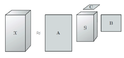
Figure 1: Tucker decomposition of a third-order tensor.

Below we present the definitions of some concepts used in this paper.

Definition 1.

(Kronecker products) The Kronecker product of matrices $A\in\mathbb{R}^{m\times n}$ and $B\in\mathbb{R}^{k\times l}$ is defined as

$$A\otimes B=\begin{bmatrix}a_{11}B&a_{12}B&...&a_{1n}B\\ a_{21}B&a_{22}B&...&a_{2n}B\\ \colon&\colon&\ddots&\colon\\ a_{m1}B&a_{m2}B&...&a_{mn}B\end{bmatrix}\in\mathbb{R}^{mk\times nl}.$$

The Kronecker product helps express Tucker decomposition. The Tucker decomposition in (2) implies

$$X_{(n)}=U^{(n)}G_{(n)}(U^{(N)}\otimes...\otimes U^{(n+1)}\otimes U^{(n-1)}\otimes...\otimes U^{(1)})^{\top}.$$

Definition 2 (Standard normal matrix).

The elements of a standard normal matrix follow the real standard normal distribution (i.e., Gaussian with mean zero and variance one) form an independent family of standard normal random variables.

Definition 3.

(Standard Gaussian tensor) The elements of a standard Gaussian tensor follow the standard Gaussian distribution.

Definition 4 (Tail energy).

The $j$th tail energy of a matrix $X$ is defined as

$$\tau_{j}^{2}({X}):=\min_{{\rm rank}({Y})<j}\|{X}-{Y}\|_{F}^{2}=\sum_{i\geq j}\sigma_{i}^{2}({X}).$$

2.2 Truncated higher-order SVD

Since the actual Tucker rank of large-scale higher-order tensor is hard to compute, the truncated Tucker decomposition with a pre-determined truncation $(r_{1},r_{2},...,r_{N})$ is widely used in practice. THOSVD is a popular approach to computing the truncated Tucker approximation, also known as the best low multilinear rank-$(r_{1},r_{2},...,r_{N})$ approximation, which reads

$$\min_{\mathcal{G}\mathchar 24635\relax\;{U}^{(1)},{U}^{(2)},\cdots,{U}^{(N)}}\|\mathcal{X}-\mathcal{G}\times_{1}{U}^{(1)}\times_{2}{U}^{(2)}\cdots\times_{N}{U}^{(N)}\|_{F}^{2}$$

$${\rm s.t.}\quad{U}^{(n)\top}{U}^{(n)}={I}_{r_{n}},n\in\{1,2,...,N\}.$$

Algorithm 1 THOSVD

1:tensor $\mathcal{X}\in\mathbb{R}^{I_{1}\times I_{2}\times\ldots\times I_{N}}$ and target rank $(r_{1},r_{2},\ldots,r_{N})$

2:Tucker approximation $\hat{\mathcal{X}}=\mathcal{G}\times_{1}{U}^{\left(1\right)}\times_{1}{U}^{\left(2\right)}\cdots\times_{N}{U}^{\left(N\right)}$

3:for $n=1,2,\ldots,N$ do

4:     $(U^{(n)},\sim,\sim)\leftarrow{\tt truncatedSVD}({X}_{(n)},r_{n})$

5:end for

6:$\mathcal{G}\leftarrow{\mathcal{X}\times}_{1}{U}^{\left(1\right)\top}\times_{2}{U}^{\left(2\right)\top}\cdots\times_{N}{U}^{\left(N\right)\top}$

Algorithm 1 summarizes the THOSVD approach. Each mode is processed individually in Algorithm 1. The low-rank factor matrices of mode-$n$ unfolding matrix $X_{(n)}$ are computed through the truncated SVD, i.e.,

$${X}_{(n)}=\begin{bmatrix}{U}^{(n)}&\tilde{{U}^{(n)}}\end{bmatrix}\begin{bmatrix}S^{(n)}&\\ &\tilde{S^{(n)}}\end{bmatrix}\begin{bmatrix}{V}^{(n)\top}\\ \tilde{{V}^{(n)\top}}\end{bmatrix}\cong{U}^{(n)}S^{(n)}{V}^{(n)\top},$$

where ${U}^{(n)}S^{(n)}{V}^{(n)\top}$ is a rank-$r_{n}$ approximation of $X_{(n)}$, the orthogonal matrix ${U}^{(n)}\in\mathbb{R}^{I_{n}\times r_{n}}$ is the mode-${n}$ factor matrix of $\mathcal{X}$ in Tucker decomposition, $S^{(n)}\in\mathbb{R}^{r_{n}\times r_{n}}$ and ${V}^{(n)}\in\mathbb{R}^{I_{1}...I_{n-1}I_{n+1}...I_{N}\times r_{n}}$. Once all factor matrices have been computed, the core tensor $\mathcal{G}$ can be computed as

$$\mathcal{G}={\mathcal{X}\times}_{1}{U}^{\left(1\right)\top}\times_{2}{U}^{\left(2\right)\top}\cdots\times_{N}{U}^{\left(N\right)\top}\in\mathbb{R}^{r_{1}\times r_{2}\times...\times r_{N}}.$$

Then, the Tucker approximation $\hat{\mathcal{X}}$ of $\mathcal{X}$ can be computed as

$$\begin{split}\hat{\mathcal{X}}=&\ \mathcal{G}\times_{1}{U}^{(1)}\times_{2}{U}^{(2)}\cdots\times_{N}{U}^{(N)}\\ =&\ \mathcal{X}\times_{1}(U^{(1)}U^{(1)\top})\times_{2}(U^{(2)}U^{(2)\top})\cdots\times_{N}(U^{(N)}U^{(N)\top}).\end{split}$$

With the notation $\Delta_{n}^{2}(\mathcal{X})\triangleq\sum_{i=r_{n}+1}^{I_{n}}\sigma_{i}^{2}({X}_{(n)})$ and $\Delta_{n}^{2}{(\mathcal{X})\leq\|\mathcal{X}-\hat{\mathcal{X}}_{\rm opt}\|_{F}^{2}}$ Minster et al2020 , the error-bound for Algorithm 1 can be stated in the following Theorem 1.

Theorem 1 (Vannieuwenhoven et al2012 , Theorem 5.1).

Let $\hat{\mathcal{X}}=\mathcal{G}\times_{1}U^{(1)}\times_{2}U^{(2)}\cdots\times_{N}U^{(N)}$ be the low multilinear rank-$(r_{1},r_{2},...,r_{N})$ approximation of a tensor $\mathcal{X}\in\mathbb{R}^{I_{1}\times I_{2}\times\ldots\times I_{N}}$ by THOSVD. Then

$$\|\mathcal{X}-\hat{\mathcal{X}}\|_{F}^{2} \leq\sum_{n=1}^{N}\|\mathcal{X}\times_{n}({I}_{I_{n}}-{U}^{(n)}{U}^{(n)\top})\|_{F}^{2}=\sum_{n=1}^{N}\sum_{i=r_{n}+1}^{I_{n}}\sigma_{i}^{2}({X}_{(n)})$$

$$=\sum_{n=1}^{N}\Delta_{n}^{2}(\mathcal{X})\leq N\|\mathcal{X}-\hat{\mathcal{X}}_{\rm opt}\|_{F}^{2}.$$

2.3 Sequentially truncated higher-order SVD

Vannieuwenhoven et al.Vannieuwenhoven et al2012 proposed one more efficient and less computationally complex approach for computing approximate Tucker decomposition of tensors, called STHOSVD. Unlike THOSVD algorithm, STHOSVD updates the core tensor simultaneously whenever a factor matrix has computed.

Given the target rank $(r_{1},r_{2},\ldots,r_{N})$ and a processing order $s_{p}:\{1,2,...,N\}$, the minimization problem (1) can be formulated as the following optimization problem

$$\min_{{U}^{(1)},\cdots,{U}^{(N)}}\|\mathcal{X}-\mathcal{X}\times_{1}(U^{(1)}U^{(1)\top})\times_{2}(U^{(2)}U^{(2)\top})\cdots\times_{N}(U^{(N)}U^{(N)\top})\|_{F}^{2}$$ (3)

$$= \min_{{U}^{(1)},\cdots,{U}^{(N)}}(\|\mathcal{X}\times_{1}(I_{1}-U^{(1)}U^{(1)\top})\|_{F}^{2}+\|\hat{\mathcal{X}}^{(1)}\times_{2}(I_{2}-U^{(2)}U^{(2)\top})\|_{F}^{2}+$$

$$\quad\quad\cdots+\|\hat{\mathcal{X}}^{(N-1)}\times_{N}(I_{N}-U^{(N)}U^{(N)\top})\|_{F}^{2})$$

$$= \min_{U^{(1)}}(\|\mathcal{X}\times_{1}(I_{1}-U^{(1)}U^{(1)\top})\|_{F}^{2}+\min_{U^{(2)}}(\|\hat{\mathcal{X}}^{(1)}\times_{2}(I_{2}-U^{(2)}U^{(2)\top})\|_{F}^{2}+$$

$$\quad\quad\min_{U^{(3)}}(\cdots+\min_{U^{(N)}}\|\hat{\mathcal{X}}^{(N-1)}\times_{N}(I_{N}-U^{(N)}U^{(N)\top})\|_{F}^{2}))),$$

where $\hat{\mathcal{X}}^{(n)}=\mathcal{X}\times_{1}(U^{(1)}U^{(1)\top})\times_{2}(U^{(2)}U^{(2)\top})\cdots\times_{n}(U^{(n)}U^{(n)\top}),n=1,2,...,N-1$, denote the intermediate approximation tensors.

Algorithm 2 STHOSVD

1:tensor $\mathcal{X}\in\mathbb{R}^{I_{1}\times I_{2}\times\ldots\times I_{N}}$, target rank $(r_{1},r_{2},\ldots,r_{N})$, and processing order $s_{p}:\{i_{1},i_{2},\ldots,i_{N}\}$

2:Tucker approximation $\hat{\mathcal{X}}=\mathcal{G}\times_{1}{U}^{(1)}\times_{2}{U}^{(2)}\ldots\times_{N}{U}^{(N)}$

3:$\mathcal{G}\leftarrow\mathcal{X}$

4:for $n=i_{1},i_{2},\ldots,i_{N}$ do

5:     $(U^{(n)},S^{(n)},V^{(n)\top})\leftarrow{\tt truncatedSVD}({G}_{(n)},r_{n})$

6:     $\mathcal{G}\leftarrow{\tt fold_{n}}(S^{(n)}V^{(n)\top})$ (% forming the updated tensor from its mode-$n$ unfolding)

7:end for

In Algorithm 2, the solution $U^{(n)}$ of problem (LABEL:pro3) can be obtained via ${\tt truncatedSVD}(G_{(n)},r_{n})$, where $G_{(n)}$ is mode-$n$ unfolding matrix of the $(n-1)$-th intermediate core tensor $\mathcal{G}=\mathcal{X}\times_{i=1}^{n-1}U^{(i)\top}\in\mathbb{R}^{r_{1}\times r_{2}\times...\times r_{n-1}\times I_{n}\times...\times I_{N}}$, i.e.,

$$G_{(n)}=\begin{bmatrix}{U}^{(n)}&\tilde{{U}^{(n)}}\end{bmatrix}\begin{bmatrix}S^{(n)}&\\ &\tilde{S^{(n)}}\end{bmatrix}\begin{bmatrix}{V}^{(n)\top}\\ \tilde{{V}^{(n)\top}}\end{bmatrix}\cong{U}^{(n)}S^{(n)}{V}^{(n)\top},$$

where the orthogonal matrix ${U}^{(n)}$ is the mode-${n}$ factor matrix, and $S^{(n)}{V}^{(n)\top}\in\mathbb{R}^{r_{n}\times r_{1}...r_{n-1}I_{n+1}...I_{N}}$ is used to update the $n$-th intermediate core tensor $\mathcal{G}$. Function ${\tt fold_{n}}(S^{(n)}V^{(n)\top})$ tensorizes matrix $S^{(n)}{V}^{(n)\top}$ into tensor $\mathcal{G}\in\mathbb{R}^{r_{1}\times r_{2}\times...\times r_{n}\times I_{n+1}\times...\times I_{N}}$. When the target rank $r_{n}$ is much smaller than $I_{n}$, the size of the updated intermediate core tensor $\mathcal{G}$ is much smaller than original tensor. This method can significantly improve computational performance. STHOSVD algorithm possesses the following error-bound.

Theorem 2 (Vannieuwenhoven et al2012 , Theorem 6.5).

Let $\hat{\mathcal{X}}=\mathcal{G}\times_{1}U^{(1)}\times_{2}U^{(2)}\ldots\times_{N}U^{(N)}$ be the low multilinear rank-$(r_{1},r_{2},...,r_{N})$ approximation of a tensor $\mathcal{X}\in\mathbb{R}^{I_{1}\times I_{2}\times\ldots\times I_{N}}$ by STHOSVD with processsing order $s_{p}:\{1,2,\ldots,N\}$. Then

$$\|\mathcal{X}-\hat{\mathcal{X}}\|_{F}^{2} =\sum_{n=1}^{N}\|\hat{\mathcal{X}}^{(n-1)}-\hat{\mathcal{X}}^{(n)}\|_{F}^{2}\leq\sum_{n=1}^{N}\|\mathcal{X}\times_{n}({I}_{I_{n}}-{U}^{(n)}{U}^{(n)\top})\|_{F}^{2}$$

$$=\sum_{n=1}^{N}\Delta_{n}^{2}(\mathcal{X})\leq N\|\mathcal{X}-\hat{\mathcal{X}}_{\rm opt}\|_{F}^{2}.$$

Although STHOSVD has the same error-bound as THOSVD, it is less computationally complex and requires less storage. As shown in Section 5 for the numerical experiment, the running (CPU) time of the STHOSVD algorithm is significantly reduced, and the approximation error has slightly better than that of THOSVD in some cases.

2.4 Randomized STHOSVD

When the dimensions of data tensors are enormous, the computational cost of the classical deterministic algorithm TSVD for finding a low-rank approximation of mode-$n$ unfolding matrix can be expensive. Randomized low-rank matrix algorithms replace original large-scale matrix with a new one through a preprocessing step. The new matrix contains as much information as possible about the rows or columns of original data matrix. Its size is smaller than original matrix, allowing the data matrix to be processed efficiently and thus reducing the memory requirements for solving low-rank approximation of large matrix.

Algorithm 3 R-SVD

1:matrix ${A}\in\mathbb{R}^{m\times n}$, target rank $r$, and oversampling parameter $p\geq 0$

2:low-rank approximation matrix $\hat{A}=\hat{U}\hat{S}\hat{V}^{\top}$ of $A$

3:$\Omega\leftarrow{\tt randn}(n,r+p)$

4:${Y}\leftarrow{A}\Omega$

5:$({Q},\sim)\leftarrow{\tt thinQR}({Y})$

6:${B}\leftarrow Q^{\top}A$

7:(${U},S,{V}^{\top})\leftarrow{\tt thinSVD}(B)$

8:$\hat{U}\leftarrow QU(:,1:r)$

9:$\hat{S}\leftarrow S(1:r,1:r),\hat{V}\leftarrow V(:,1:r)$

N. Halko et al. Halko et al2011 proposed a randomized SVD (R-SVD) for matrices. The preprocessing stage of the algorithm is performed by right multiplying original data matrix ${A}\in\mathbb{R}^{m\times n}$ with a random Gaussian matrix $\Omega\in\mathbb{R}^{n\times r}$. Each column of the resulting new matrix $Y=A\Omega\in\mathbb{R}^{m\times r}$ is a linear combination of the columns of original data matrix. When $r<n$, the size of matrix $Y$ is smaller than $A$. The oversampling technique can improve the accuracy of solutions. Subsequent computations are summarised in Algorithm 3, where randn generates a Gaussian random matrix, thinQR produces an economy-size of the QR decomposition, and thinSVD is the thin SVD decomposition. When $A$ is dense, the arithmetic cost of Algorithm 3 is $\mathcal{O}(2(r+p)mn+r^{2}(m+n))$ flops, where $p>0$ is the oversampling parameter satisfying $r+p\leq\min\{m,n\}$.

Algorithm 3 is an efficient randomized algorithm for computing rank-$r$ approximations to matrices. Minster et al. Minster et al2020 applied Algorithm 3 directly to the STHOSVD algorithm and then presented a randomized version of STHOSVD (i.e., R-STHOSVD), see Algorithm 4.

Algorithm 4 R-STHOSVD

1:tensor $\mathcal{X}\in\mathbb{R}^{I_{1}\times I_{2}\times\ldots\times I_{N}}$, targer rank $(r_{1},r_{2},\ldots,r_{N})$, processing order $s_{p}:\{i_{1},i_{2},\ldots,i_{N}\}$, and oversampling parameter $p\geq 0$

2:Tucker approximation $\hat{\mathcal{X}}=\mathcal{G}\times_{1}{U}^{\left(1\right)}\times_{2}{U}^{\left(2\right)}\ldots\times_{N}{U}^{\left(N\right)}$

3:$\mathcal{G}\leftarrow\mathcal{X}$

4:for $n=i_{1},i_{2},\ldots,i_{N}$ do

5:     $(\hat{U},\hat{S},\hat{V}^{\top})\leftarrow$ R-SVD$({G}_{(n)},r_{n},p)$ (cf. Algorithm 3)

6:     ${U}^{\left(n\right)}\leftarrow{\hat{U}}$

7:     $\mathcal{G}\leftarrow{\tt fold_{n}}(\hat{S}\hat{V}^{\top})$

8:end for

3 Sketching algorithm for STHOSVD

A drawback of R-SVD algorithm is that when both dimensions of the intermediate matrices are enormous, the computational cost can still be high. To resolve this problem, we could resort to the two-sided sketching algorithm for low-rank matrix approximation proposed by Joel A. Tropp et al. Tropp et al2017 . The preprocessing of sketching algorithm needs two sketch matrices to contain information regarding the rows and columns of input matrix ${A}\in\mathbb{R}^{m\times n}$. Thus we should choose two sketch size parameters $k$ and $l$, s.t. , $r\leq k\leq\min\{l,n\}$, $0<l\leq m$. The random matrices $\Omega\in\mathbb{R}^{n\times k}$ and $\Psi\in\mathbb{R}^{l\times m}$ are fixed independent standard normal matrices. Then we can multiply matrix ${A}$ left and right respectively to obtain random sketch matrices ${Y}\in\ \mathbb{R}^{m\times k}$ and ${W}\in\mathbb{R}^{l\times n}$, which collect sufficient data about the input matrix to compute the low-rank approximation. The dimensionality and distribution of the random sketch matrices determine the approximation’s potential accuracy, with larger values of $k$ and $l$ resulting in better approximations but also requiring more storage and computational cost.

Algorithm 5 Sketch for low-rank approximation

1:matrix ${A}\in\mathbb{R}^{m\times n}$, and sketch size parameters $k,l$

2:rank-$k$ approximation $\hat{{A}}={Q}{X}$ of $A$

3:$\Omega\leftarrow{\tt randn}(n,k),\Psi\leftarrow{\tt randn}(l,m)$

4:$\Omega\leftarrow{\tt orth}(\Omega),{\Psi^{\top}\leftarrow{\tt orth}(\Psi^{\top})}$

5:${Y}\leftarrow{A}\Omega$

6:${W}\leftarrow\Psi{A}$

7:$({Q},\sim)\leftarrow{\tt thinQR}({Y})$

8:${X}\leftarrow(\Psi{Q})^{\dagger}{W}$

The sketching algorithm for low-rank approximation is given in Algorithm 5. Function ${\tt orth}(A)$ in Step 2 produces an orthonormal basis of A. Using orthogonalization matrices will achieve smaller errors and better numerical stability than directly using the randomly generated Gaussian matrices. In particular, when $A$ is dense, the arithmetic cost of Algorithm 5 is $\mathcal{O}((k+l)mn+kl(m+n))$ flops. Algorithm 5 is simple, practical, and possesses the sub-optimal error-bound as stated in the following Theorem 3. In Theorem 3, function $f(s,t):=s/(t-s-1)(t>s+1>1)$. The minimum in Theorem 3 reveals that the low rank approximation of given matrix $A$ automatically exploits the decay of tail energy.

Theorem 3 (Tropp et al2017 , Theorem 4.3).

Assume that the sketch size parameters satisfy $l>k+1$, and draw random test matrices $\Omega\in\mathbb{R}^{n\times k}$ and $\Psi{\in\mathbb{R}}^{l\times m}$ independently forming the standard normal distribution. Then the rank-$k$ approximation $\hat{{A}}$ obtained from Algorithm 5 satisfies

$$\mathbb{E}\parallel{A}-\hat{{A}}\parallel_{F}^{2} \leq(1+f(k,l))\cdot\min_{\varrho<k-1}(1+f(\varrho,k))\cdot\tau_{\varrho+1}^{2}({A})$$

$$=\frac{k}{l-k-1}\cdot\min_{\varrho<k-1}\frac{k}{k-\varrho-1}\cdot\tau_{\varrho+1}^{2}({A}).$$

Using the two-sided sketching algorithm to leverage STHOSVD algorithm, we propose a practical sketching algorithm for STHOSVD named Sketch-STHOSVD. We summarize the procedures of Sketch-STHOSVD algorithm in Algorithm 6, with its error analysis stated in Theorem 4.

Algorithm 6 Sketch-STHOSVD

1:tensor $\mathcal{X}\in\mathbb{R}^{I_{1}\times I_{2}\times\ldots\times I_{N}}$, targer rank $(r_{1},r_{2},\ldots,r_{N})$, processing order $s_{p}:\{i_{1},i_{2},\ldots,i_{N}\}$, and sketch size parameters $\{l_{1},l_{2},...,l_{N}\}$

2:Tucker approximation $\hat{\mathcal{X}}=\mathcal{G}\times_{1}{U}^{\left(1\right)}\times_{2}{U}^{\left(2\right)}\ldots\times_{N}{U}^{\left(N\right)}$

3:$\mathcal{G}\leftarrow\mathcal{X}$

4:for  $n=i_{1},i_{2},\ldots,i_{N}$  do

5:     $({Q},{X})\leftarrow$ Sketch$({G}_{(n)},r_{n},l_{n})$ (cf. Algorithm 5)

6:     ${U}^{\left(n\right)}\leftarrow{Q}$

7:     $\mathcal{G}\leftarrow{\tt fold_{n}}(X)$

8:end for

Theorem 4.

Let $\hat{\mathcal{X}}=\mathcal{G}\times_{1}{U}^{(1)}\times_{2}{U}^{(2)}\ldots\times_{N}{U}^{(N)}$ be the Tucker approximation of a tensor $\mathcal{X}\in\mathbb{R}^{I_{1}\times I_{2}\times\ldots\times I_{N}}$ by the Sketch-STHOSVD algorithm (i.e., Algorithm 6) with target rank $r_{n}<I_{n},n=1,2,...,N$, sketch size parameters $\{l_{1},l_{2},...,l_{N}\}$ and processing order $s_{p}:\{1,2,\ldots,N\}$. Then

$$\mathbb{E}_{\{\Omega_{j}\}_{j=1}^{N}}\|\mathcal{X}-\widehat{\mathcal{X}}\|_{F}^{2} \leq{\sum\limits_{n=1}^{N}\frac{r_{n}}{l_{n}-r_{n}-1}\min_{\varrho_{n}<r_{n}-1}\frac{r_{n}}{r_{n}-\varrho_{n}-1}\Delta_{n}^{2}({\cal X})}$$

$$\leq\sum\limits_{n=1}^{N}\frac{r_{n}}{l_{n}-r_{n}-1}\min_{\varrho_{n}<r_{n}-1}\frac{r_{n}}{r_{n}-\varrho_{n}-1}\|\mathcal{X}-\hat{\mathcal{X}}_{\rm opt}\|_{F}^{2}.$$

Proof: Combining Theorem 2 and Theorem 3, we have

$$\ \mathbb{E}_{\{\Omega_{j}\}_{j=1}^{N}}\|\mathcal{X}-\widehat{\mathcal{X}}\|_{F}^{2}$$

$$= \sum\limits_{n=1}^{N}\mathbb{E}_{\{\Omega_{j}\}_{j=1}^{N}}\|\hat{\mathcal{X}}^{(n-1)}-\hat{\mathcal{X}}^{(n)}\|_{F}^{2}$$

$$= \sum\limits_{n=1}^{N}\mathbb{E}_{\{\Omega_{j}\}_{j=1}^{n-1}}\left\{\mathbb{E}_{\Omega_{n}}\|\hat{\mathcal{X}}^{(n-1)}-\hat{\mathcal{X}}^{(n)}\|_{F}^{2}\right\}$$

$$= \sum\limits_{n=1}^{N}\mathbb{E}_{\{\Omega_{j}\}_{j=1}^{n-1}}\left\{\mathbb{E}_{\Omega_{n}}\|\mathcal{G}^{(n-1)}\times_{i=1}^{n-1}{{U}^{(i)}}{\times_{n}}({I}-{{U}^{(n)}}{U}^{(n)\top})\|_{F}^{2}\right\}$$

$$\leq \sum\limits_{n=1}^{N}\mathbb{E}_{\{\Omega_{j}\}_{j=1}^{n-1}}\left\{\mathbb{E}_{\Omega_{n}}\|({I}-{{U}^{(n)}}{U}^{(n)\top}){G}_{n}^{n-1})\|_{F}^{2}\right\}$$

$$\leq \sum\limits_{n=1}^{N}\mathbb{E}_{\{\Omega_{j}\}_{j=1}^{n-1}}\frac{r_{n}}{l_{n}-r_{n}-1}\min_{\varrho_{n}<r_{n}-1}\frac{r_{n}}{r_{n}-\varrho_{n}-1}\sum\limits_{i=r_{n}+1}^{I_{n}}\sigma_{i}^{2}({G}_{(n)}^{(n-1)})$$

$$\leq \sum\limits_{n=1}^{N}\mathbb{E}_{\{\Omega_{j}\}_{j=1}^{n-1}}\frac{r_{n}}{l_{n}-r_{n}-1}\min_{\varrho_{n}<r_{n}-1}\frac{r_{n}}{r_{n}-\varrho_{n}-1}\Delta_{n}^{2}({\cal X})$$

$$= \sum\limits_{n=1}^{N}\frac{r_{n}}{l_{n}-r_{n}-1}\min_{\varrho_{n}<r_{n}-1}\frac{r_{n}}{r_{n}-\varrho_{n}-1}\Delta_{n}^{2}({\cal X})$$

$$\leq {\sum\limits_{n=1}^{N}\frac{r_{n}}{l_{n}-r_{n}-1}\min_{\varrho_{n}<r_{n}-1}\frac{r_{n}}{r_{n}-\varrho_{n}-1}}\|\mathcal{X}-\hat{\mathcal{X}}_{\rm opt}\|_{F}^{2}.$$

We assume the processing order for STHOSVD, R-STHOSVD, and Sketch-STHOSVD algorithms is $s_{p}:\{1,2,...,N\}$. Table 2 summarises the arithmetic cost of different algorithms for the cases related to the general higher-order tensor $\mathcal{X}\in\mathbb{R}^{I_{1}\times I_{2}\times...\times I_{N}}$ with target rank $(r_{1},r_{2},\ldots,r_{N})$ and the special cubic tensor $\mathcal{X}\in\mathbb{R}^{I\times I\times...\times I}$ with target rank $(r,r,...,r)$. Here the tensors are dense and the target ranks $r_{j}\ll I_{j},j=1,2,\ldots,N$.

Table 2: Arithmetic cost for the algorithms THOSVD, STHOSVD, R-STHOSVD, and the proposed Sketch-STHOSVD.

Algorithm	$\mathcal{X}\in\mathbb{R}^{I_{1}\times I_{2}\times...\times I_{N}}$	$\mathcal{X}\in\mathbb{R}^{I\times I\times...\times I}$
THOSVD	$\mathcal{O}(\sum\limits_{j=1}^{N}I_{j}I_{1:N}+\sum_{j=1}^{N}r_{1:j}I_{j:N})$	$\mathcal{O}(NI^{N+1}+\sum\limits_{j=1}^{N}r^{j}I^{N-j+1})$
STHOSVD	$\mathcal{O}(\sum\limits_{j=1}^{N}I_{j}r_{1:j-1}I_{j:N}+\sum\limits_{j=1}^{N}r_{1:j}I_{j+1:N})$	$\mathcal{O}(\sum\limits_{j=1}^{N}r^{j-1}I^{N-j+2}+r^{j}I^{N-j})$
R-STHOSVD	$\mathcal{O}(\sum\limits_{j=1}^{N}r_{1:j}I_{j:N}+\sum\limits_{j=1}^{N}r_{1:j}I_{j+1:N})$	$\mathcal{O}(\sum\limits_{j=1}^{N}r^{j}I^{N-j+1}+r^{j}I^{N-j})$
Sketch-STHOSVD	$\mathcal{O}(\sum\limits_{j=1}^{N}r_{j}l_{j}(I_{j}+r_{1:j-1}I_{j+1:N})+\sum\limits_{j=1}^{N}r_{1:j}I_{j+1:N})$	$\mathcal{O}(\sum\limits_{j=1}^{N}rl(I+r^{j-1}I^{N-j})+r^{j}I^{N-j})$

4 Sketching algorithm with subspace power iteration

When the size of original matrix is very large or the singular spectrum of original matrix decays slowly, Algorithm 5 may produce a poor basis in many applications. Inspired by Rokhlin et al2009 , we suggest using the power iteration technique to enhance the sketching algorithm by replacing ${A}$ with $({A}{A}^{\top})^{q}{A}$, where $q$ is a positive integer. According to the SVD decomposition of matrix ${A}$, i.e., ${A}={U}{S}{V}^{\top}$, we know that $({A}{A}^{\top})^{q}{A}={U}{S}^{2q+1}{V}^{\top}$. It can see that ${A}$ and $({A}{A}^{\top})^{q}{A}$ have the same left and right singular vectors, but the latter has a faster decay rate of singular values, making its tail energy much smaller.

Algorithm 7 Sketching algorithm with subspace power iteration (sub-Sketch)

1:matrix ${A}\in\mathbb{R}^{m\times n}$, sketch size parameters $k,l$, and integer $q>0$

2:rank-$k$ approximation $\hat{{A}}={Q}{X}$ of $A$

3:$\Omega\leftarrow{\tt randn}(n,k),\Psi\leftarrow{\tt randn}(l,m)$

4:$\Omega\leftarrow{\tt orth}(\Omega),\Psi^{\top}\leftarrow{\tt orth}(\Psi^{\top})$

5:${Y}={A}\Omega$, ${W}=\Psi{A}$

6:$Q_{0}\leftarrow{\tt thinQR}(Y)$

7:for $j=1,\ldots,q$ do

8:     $\hat{{Y}}_{j}={A}^{\top}{Q_{j-1}}$

9:     $(\hat{{Q}}_{j},\sim)\leftarrow{\tt thinQR}(\hat{{Y}}_{j})$

10:     ${Y}_{j}={A}\hat{{Q}}_{j}$

11:     $({Q}_{j},\sim)\leftarrow{\tt thinQR}({Y}_{j})$

12:end for

13:${Q}={Q}_{q}$

14:$X\leftarrow(\Psi Q)^{\dagger}W$

Although power iteration can improve the accuracy of Algorithm 5 to some extent, it still suffers from a problem, i.e., during the execution with power iteration, the rounding errors will eliminate all information about the singular modes associated with the singular values. To address this issue, we propose an improved sketching algorithm by orthonormalizing the columns of the sample matrix between each application of $A$ and $A^{\top}$, see Algorithm 7. When $A$ is dense, the arithmetic cost of Algorithm 7 is $\mathcal{O}((q+1)(k+l)mn+kl(m+n))$ flops. Numerical experiments show that a good approximation can achieve with a choice of 1 or 2 for subspace power iteration parameter Halko et al2011 .

Algorithm 8 sub-Sketch-STHOSVD

1:tensor $\mathcal{X}\in\mathbb{R}^{I_{1}\times I_{2}\times\ldots\times I_{N}}$, targer rank $(r_{1},r_{2},\ldots,r_{N})$, processing order $s_{p}:\{i_{1},i_{2},\ldots,i_{N}\}$, sketch size parameters $\{l_{1},l_{2},...,l_{N}\}$, and integer $q>0$

2:Tucker approximation $\hat{\mathcal{X}}=\mathcal{G}\times_{1}{U}^{\left(1\right)}\times_{2}{U}^{\left(2\right)}\ldots\times_{N}{U}^{\left(N\right)}$

3:$\mathcal{G}\leftarrow\mathcal{X}$

4:for  $n=i_{1},i_{2},\ldots,i_{N}$ do

5:     $({Q},{X})\leftarrow$ sub-Sketch$({G}_{(n)},r_{n},l_{n},q)$ (cf. Algorithm 7)

6:     ${U}^{\left(n\right)}\leftarrow{Q}$

7:     $\mathcal{G}\leftarrow{\tt fold_{n}}(X)$

8:end for

Using Algorithm 7 to compute the low-rank approximations of intermediate matrices, we can obtain an improved sketching algorithm for STHOSVD, called sub-Sketch-STHOSVD, see Algorithm 8. The error-bound for Algorithm 8 states in the following Theorem 5. Its proof is deferred in Appendix.

Theorem 5.

Let $\hat{\mathcal{X}}=\mathcal{G}\times_{1}{U}^{(1)}\times_{2}{U}^{(2)}\ldots\times_{N}{U}^{(N)}$ be the Tucker approximation of a tensor $\mathcal{X}\in\mathbb{R}^{I_{1}\times I_{2}\times\ldots\times I_{N}}$ obtained by the sub-Sketch-STHOSVD algorithm (i.e., Algorithm 8) with target rank $r_{n}<I_{n},n=1,2,...,N$, sketch size parameters $\{l_{1},l_{2},...,l_{N}\}$ and processing order $p:\{1,2,\ldots,N\}$. Let ${\varpi_{k}}\equiv\frac{\sigma_{k+1}}{\sigma_{k}}$ denote the singular value gap, then

$$\mathbb{E}_{\{\Omega_{j}\}_{j=1}^{N}}\|\mathcal{X}-\widehat{\mathcal{X}}\|_{F}^{2} \leq{\sum\limits_{n=1}^{N}(1+f(r_{n},l_{n}))\cdot\min_{\varrho_{n}<r_{n}-1}(1+f(\varrho_{n},r_{n}){\varpi_{r}}^{4q})\cdot\tau_{\varrho+1}^{2}({X_{(n)}})}$$

$$\leq\sum\limits_{n=1}^{N}(1+f(r_{n},l_{n}))\cdot\min_{\varrho_{n}<r_{n}-1}(1+f(\varrho_{n},r_{n}){\varpi_{r}}^{4q})\|\mathcal{X}-\hat{\mathcal{X}}_{\rm opt}\|_{F}^{2}.$$

Proof: See Appendix.

5 Numerical experiments

This section conducts numerical experiments with synthetic data and real-world data, including comparisons between the traditional THOSVD, STHOSVD algorithms, the R-STHOSVD algorithm proposed in Minster et al2020 , and our proposed algorithms Sketch-STHOSVD and sub-Sketch-STHOSVD. Regarding the numerical settings, the oversampling parameter $p=5$ is used in Algorithm 3, the sketch parameters $l_{n}=r_{n}+2,n=1,2,\ldots,N$, are used in Algorithms 6 and 8, and the power iteration parameter $q=1$ is used in Algorithm 8.

5.1 Hilbert tensor

Hilbert tensor is a synthetic and supersymmetric tensor, with each entry defined as

$$\mathcal{X}_{{i_{1}}{i_{2}}...{i_{n}}}=\frac{1}{{{i_{1}}+{i_{2}}+...+{i_{n}}}},1\leq{i_{n}}\leq{I_{n}},n=1,2,...,N.$$

In the first experiment, we set $N=5$ and $I_{n}=25,n=1,2,\ldots,N$. The target rank is chosen as $(r,r,r,r,r)$, where $r\in[1,25]$. Due to the supersymmetry of the Hilbert tensor, the processing order in the algorithms does not affect the final experimental results, and thus the processing order can be directly chosen as $s_{p}:\{1,2,3,4,5\}$.

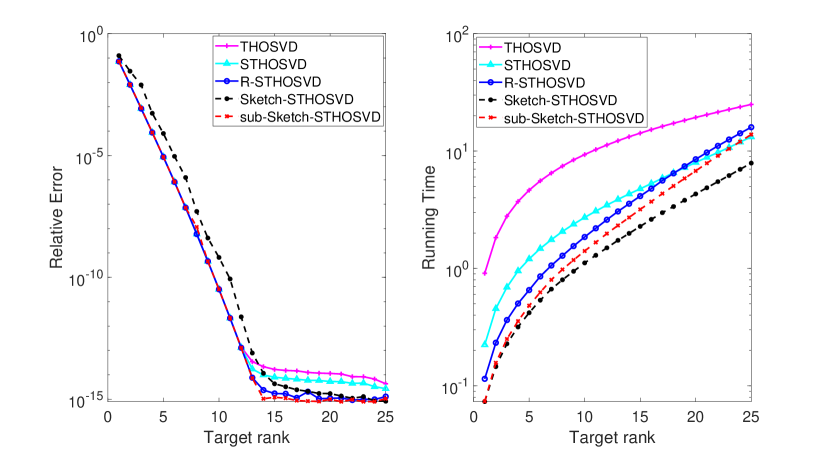
Figure 2: Results comparison on the Hilbert tensor with a size of $25\times 25\times 25\times 25\times 25$ in terms of numerical error (left) and CPU time (right).

The results of different algorithms are given in Figure 2. It shows that our proposed algorithms (i.e., Sketch-STHOSVD and sub-Sketch-STHOSVD) and algorithm R-STHOSVD outperform the algorithms THOSVD and STHOSVD. In particular, the error of the proposed algorithms Sketch-STHOSVD and sub-Sketch-STHOSVD is comparable to R-STHOSVD (see the left plot in Figure 2), while they both use less CPU time than R-STHOSVD (see the right plot in Figure 2). This result demonstrates the excellent performance of the proposed algorithms and indicates that the two-sided sketching method and the subspace power iteration used in our algorithms can indeed improve the performance of STHOSVD algorithm.

For a large-scale test, we use a Hilbert tensor with a size of $500\times 500\times 500$ and conduct experiments using ten different approximate multilinear ranks. We perform the tests ten times and report the algorithms’ average running time and relative error in Table 3 and Table 4, respectively. The results show that the randomized algorithms can achieve higher accuracy than the deterministic algorithms. The proposed Sketch-STHOSVD algorithm is the fastest, and the sub-Sketch-STHOSVD algorithm achieves the highest accuracy efficiently.

Table 3: Results comparison in terms of the CPU time (in second) on the Hilbert tensor with a size of $500\times 500\times 500$ as the target rank increases.

Target rank	THOSVD	STHOSVD	R-STHOSVD	Sketch-STHOSVD	sub-Sketch-STHOSVD
(10,10,10)	17.18	7.49	0.92	0.86	0.98
(20,20,20)	23.13	8.87	1.25	1.05	1.48
(30,30,30)	24.91	9.35	1.66	1.53	2.16
(40,40,40)	28.05	10.41	1.94	1.44	2.11
(50,50,50)	29.44	11.39	2.07	1.67	2.43
(60,60,60)	30.14	11.07	2.37	1.90	2.77
(70,70,70)	29.44	11.18	2.57	2.10	3.02
(80,80,80)	29.65	12.30	3.05	2.54	3.75
(90,90,90)	31.11	12.80	3.80	2.80	4.33
(100,100,100)	32.22	13.51	4.04	3.07	4.61

Table 4: Results comparison in terms of the relative error on the Hilbert tensor with a size of $500\times 500\times 500$ as the target rank increases.

Target rank	THOSVD	STHOSVD	R-STHOSVD	Sketch-STHOSVD	sub-Sketch-STHOSVD
(10,10,10)	2.7354e-06	2.7347e-06	2.7347e-06	1.1178e-05	2.7568e-06
(20,20,20)	1.1794e-12	1.1793e-12	1.1794e-12	7.1408e-12	1.2677e-12
(30,30,30)	4.6574e-15	3.2739e-15	3.2201e-15	4.0641e-15	2.0182e-15
(40,40,40)	4.4282e-15	3.4249e-15	2.8212e-15	2.1562e-15	1.7860e-15
(50,50,50)	4.1628e-15	3.2342e-15	2.6823e-15	2.3205e-15	1.8625e-15
(60,60,60)	4.1214e-15	3.1271e-15	2.3652e-15	2.2920e-15	1.7472e-15
(70,70,70)	4.1085e-15	3.0000e-15	2.1761e-15	2.0499e-15	1.6370e-15
(80,80,80)	4.0956e-15	3.1350e-15	1.8382e-15	1.8209e-15	1.6424e-15
(90,90,90)	4.0792e-15	3.3742e-15	1.8102e-15	1.7193e-15	1.5264e-15
(100,100,100)	4.0390e-15	3.0571e-15	1.7323e-15	1.6304e-15	1.4957e-15

5.2 Sparse tensor

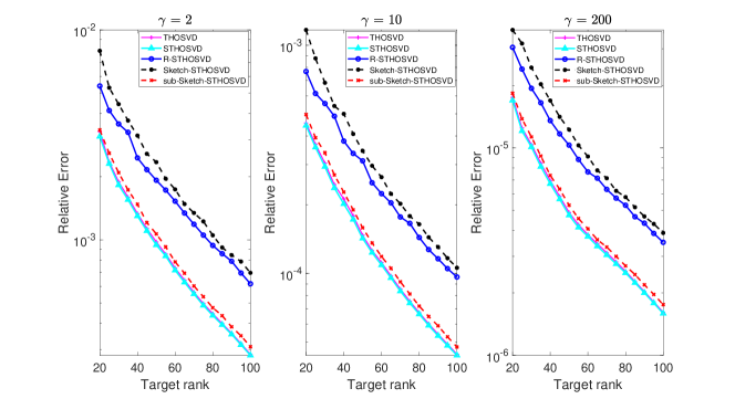
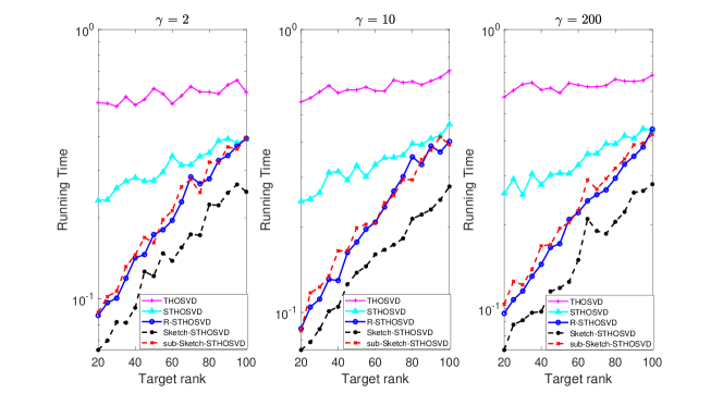
Figure 3: Results comparison on a sparse tensor with a size of $200\times 200\times 200$ in terms of numerical error (first row) and CPU time (second row).

In this experiment, we test the performance of different algorithms on a sparse tensor $\mathcal{X}\in\mathbb{R}^{200\times 200\times 200}$, i.e.,

$$\mathcal{X}=\sum\limits_{i=1}^{10}{\frac{\gamma}{{{i^{2}}}}}{{\bf{x}}_{i}}\circ{{\bf{y}}_{i}}\circ{{\bf{z}}_{i}}+\sum\limits_{i=11}^{200}{\frac{1}{{{i^{2}}}}}{{\bf{x}}_{i}}\circ{{\bf{y}}_{i}}\circ{{\bf{z}}_{i}}.$$

Where ${\bf{x}}_{i},{{\bf{y}}_{i}},{{\bf{z}}_{i}}\in\mathbb{R}^{n}$ are sparse vectors all generated using the sprand command in MATLAB with $5\%$ nonzeros each, and $\gamma$ is a user-defined parameter which determines the strength of the gap between the first ten terms and the rest terms. The target rank is chosen as $(r,r,r)$, where $r\in[20,100]$. The experimental results show in Figure 3, in which three different values $\gamma=2,10,200$ are tested. The increase of gap means that the tail energy will be reduced, and the accuracy of the algorithms will be improved. Our numerical experiments also verified this result.

Figure 3 demonstrates the superiority of the proposed sketching algorithms. In particular, we see that the proposed Sketch-STHOSVD is the fastest algorithm, with a comparable error against R-STHOSVD; the proposed sub-Sketch-STHOSVD can reach the same accuracy as the STHOSVD algorithm but in much less CPU time; and the proposed sub-Sketch-STHOSVD achieves much better low-rank approximation than R-STHOSVD with similar CPU time.

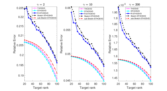
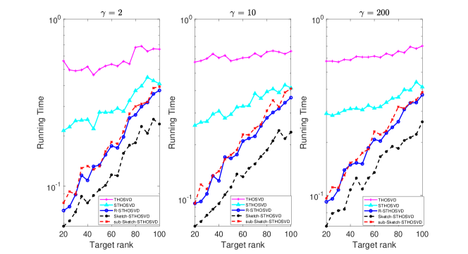
Figure 4: Results comparison on a $200\times 200\times 200$ sparse tensor with noise in terms of numerical error (first row) and CPU time (second row).

Now we consider the influence of noise on algorithms’ performance. Specifically, the sparse tensor $\mathcal{X}$ with noise is designed in the same manner as in Xiao et al2021 , i.e.,

$$\hat{\mathcal{X}}=\mathcal{X}+\delta\mathcal{K},$$

where $\mathcal{K}$ is a standard Gaussian tensor and $\delta$ is used to control the noise level. Let $\delta=10^{-3}$ and keep the rest parameters the same as the settings in the previous experiment. The relative error and running time of different algorithms are shown in Figure 4. In Figure 4, we see that noise indeed affects the accuracy of the low-rank approximation, especially when the gap is small. However, the influence of noise does not change the conclusion obtained on the case without noise. The accuracy of our sub-Sketch-STHOSVD algorithm is the highest among the randomized algorithms. As $\gamma$ increases, sub-Sketch-STHOSVD can achieve almost the same accuracy as that of THOSVD and STHOSVD in a comparable CPU time against R-STHOSVD.

5.3 Real-world data tensor

In this experiment, we test the performance of different algorithms on a colour image, called HDU picture, with a size of $1200\times 1800\times 3$. We also evaluate the proposed sketching algorithms on the widely used YUV Video Sequences. Taking the ‘hall monitor’ video as an example and using the first 30 frames, a three order tensor with a size of $144\times 176\times 30$ is then formed for this test.

Firstly, we conduct an experiment on the HDU picture with target rank $(500,500,3)$, and compare the PSNR and CPU time of different algorithms. The experimental result is shown in Figure 5, which shows that the PSNR of sub-Sketch-STHOSVD, THOSVD and STHOSVD is very similar (i.e., $\sim$ 40) and that sub-Sketch-STHOSVD is more efficient in terms of CPU time. R-STHOSVD and Sketch-STHOSVD are also very efficient compared to sub-Sketch-STHOSVD; however, the PSNR they achieve is 5 dB less than sub-Sketch-STHOSVD. Then we conduct separate numerical experiments on the HDU picture and the ‘hall monitor’ video clip as the target rank increases, and compare these algorithms in terms of the relative error, CPU time and PSNR, see Figure 6 and Figure 7. These experimental results again demonstrate the superiority (i.e., low error and good approximation with high efficiency) of the proposed sub-Sketch-STHOSVD algorithm in computing the Tucker decomposition approximation.

Original	THOSVD (2.62; 40.61)	STHOSVD (1.89; 40.65)
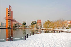
R-STHOSVD	Sketch-STHOSVD	sub-Sketch-STHOSVD
(0.61; 34.72)	(0.55; 34.63)	(0.84; 39.97)

Figure 5: Results comparison on a HDU picture with a size of $1200\times 1800\times 3$ in terms of PSNR (i.e., peak signal-to-noise ratio) and CPU time. The target rank is (500,500,3). The two values in e.g. (2.62; 40.61) represent the CPU time and the PSNR, respectively.

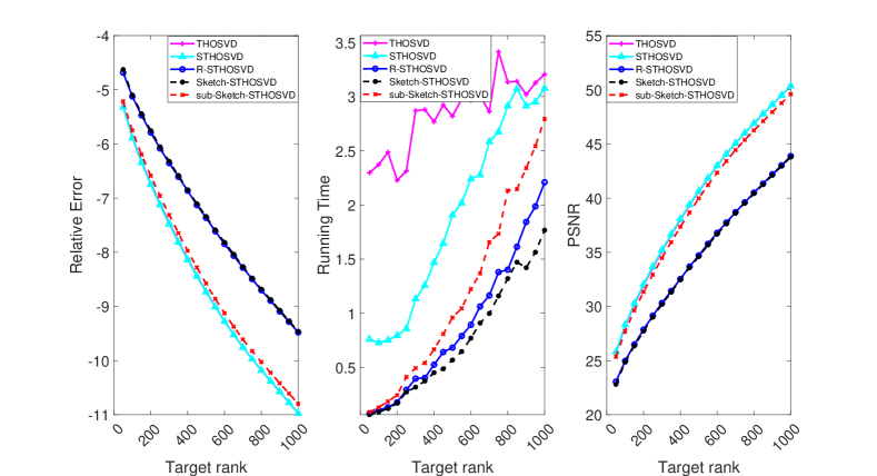
Figure 6: Results comparison on a HDU picture with size of $1200\times 1800\times 3$ in terms of numerical error (left), CPU time (middle) and PSNR (right). The HDU picture is with target rank $(r,r,3),r\in[50,1000]$.

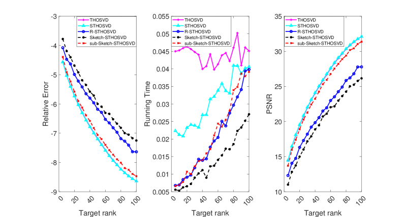
Figure 7: Results comparison on the ‘hall monitor’ grey video with size of $144\times 176\times 30$ in terms of numerical error (left), CPU time (middle) and PSNR (right). The ‘hall monitor’ grey video is with target rank $(r,r,10)$, $r\in[5,100]$.

In the last experiment, a larger-scale real-world tensor data is used. We choose a color image (called the LONDON picture) with a size of $4775\times 7155\times 3$ as the test image and consider the influence of noise. The LONDON picture with white Gaussian noise is generated using the awgn(X,SNR) built-in function in MATLAB. We set the target rank as (50,50,3) and SNR to 20. The results comparisons without and with white Gaussian noise are respectively shown in Figure 8 and Figure 9 in terms of the CPU time and PSNR. Moreover, we also test the algorithms on the LONDON picture as the target rank increases. The results regarding the relative error, the CPU time and the PSNR are reported in Tables 5, 6 and 7, respectively. On the whole, the results again show the consistent performance of the proposed methods.

Original	THOSVD (154.95; 24.07)	STHOSVD (49.34; 24.09)
R-STHOSVD	Sketch-STHOSVD	sub-Sketch-STHOSVD
(1.29; 21.27)	(1.17; 21.09)	(1.29; 23.65)

Figure 8: Results comparison on LONDON picture with a size of $4775\times 7155\times 3$ in terms of CPU time and PSNR. The target rank is (50,50,3).

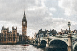
Noisy picture(PSNR=16.92)	THOSVD (160.59; 20.54)	STHOSVD (50.16; 20.54)
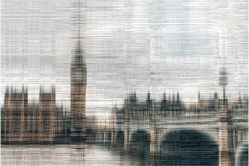
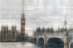
R-STHOSVD	Sketch-STHOSVD	sub-Sketch-STHOSVD
(1,25; 19.37)	(1.15; 19.25)	(1.45; 20.45)

Figure 9: Results comparison on LONDON picture with a size of $4775\times 7155\times 3$ and white Gaussian noise in terms of CPU time and PSNR. The target rank is (50,50,3).

Table 5: Results comparison in terms of the relative error on the LONDON picture with a size of $4775\times 7155\times 3$ as the target rank increases.

Target rank	THOSVD	STHOSVD	R-STHOSVD	Sketch-STHOSVD	sub-Sketch-STHOSVD
(10,10,10)	0.019037	0.019025	0.031000	0.040006	0.020756
(20,20,20)	0.012669	0.012644	0.023467	0.027398	0.013703
(30,30,30)	0.010168	0.010124	0.018354	0.020451	0.010965
(40,40,40)	0.008630	0.008599	0.015792	0.017029	0.009443
(50,50,50)	0.007576	0.007532	0.013917	0.015333	0.008286
(60,60,60)	0.006778	0.006710	0.012967	0.013589	0.007359
(70,70,70)	0.006119	0.006049	0.011813	0.011886	0.006687
(80,80,80)	0.005532	0.005491	0.010658	0.011148	0.006123
(90,90,90)	0.005076	0.005023	0.010018	0.010378	0.005602
(100,100,100)	0.004669	0.004619	0.009249	0.009578	0.005172

Table 6: Results comparison in terms of the CPU time (in second) on the LONDON picture with a size of $4775\times 7155\times 3$ as the target rank increases.

Target rank	THOSVD	STHOSVD	R-STHOSVD	Sketch-STHOSVD	sub-Sketch-STHOSVD
(10,10,10)	156.13	49.22	0.94	0.99	1.12
(20,20,20)	165.22	77.64	1.24	1.48	1.56
(30,30,30)	241.11	76.57	1.69	1.39	1.69
(40,40,40)	242.08	74.25	1.57	1.45	1.68
(50,50,50)	268.71	72.85	1.51	1.45	1.80
(60,60,60)	265.52	77.80	1.75	1.51	2.26
(70,70,70)	241.95	77.82	1.93	1.78	2.24
(80,80,80)	264.86	73.53	1.86	1.74	2.31
(90,90,90)	274.73	72.67	1.93	1.83	2.16
(100,100,100)	283.88	86.42	2.24	2.20	2.46

Table 7: Results comparison in terms of the PSNR on the LONDON picture with a size of $4775\times 7155\times 3$ as the target rank increases.

Target rank	THOSVD	STHOSVD	R-STHOSVD	Sketch-STHOSVD	sub-Sketch-STHOSVD
(10,10,10)	20.06	20.07	17.96	16.86	19.70
(20,20,20)	21.84	21.84	19.18	18.51	21.50
(30,30,30)	22.79	22.81	20.25	19.78	22.46
(40,40,40)	23.50	23.52	20.90	20.57	23.11
(50,50,50)	24.07	24.09	21.45	21.03	23.68
(60,60,60)	24.55	24.60	21.76	21.55	24.20
(70,70,70)	25.00	25.05	22.16	22.13	24.61
(80,80,80)	25.43	25.47	22.61	22.41	25.00
(90,90,90)	25.81	25.85	22.87	22.72	25.38
(100,100,100)	26.17	26.22	23.22	23.07	25.73

In summary, the numerical results show the superiority of the sub-sketch STHOSVD algorithm for large-scale tensors with or without noise. We can see that sub-Sketch-STHOSVD could achieve close approximations to that of the deterministic algorithms in a time similar to other randomized algorithms.

6 Conclusion

In this paper we proposed efficient sketching algorithms, i.e., Sketch-STHOSVD and sub-Sketch-STHOSVD, to calculate the low-rank Tucker approximation of tensors by combining the two-sided sketching technique with the STHOSVD algorithm and using the subspace power iteration. Detailed error analysis is also conducted. Numerical results on both synthetic and real-world data tensors demonstrate the competitive performance of the proposed algorithms in comparison to the state-of-the-art algorithms.

Appendix

Lemma 1.

[Zhang et al2016 , Theorem 2] Let $\varrho<k-1$ be a positive natural number and $\Omega\in\mathbb{R}^{k\times n}$ be a Gaussian random matrix. Suppose $Q$ is obtained from Algorithm 7. Then $\forall A\in\mathbb{R}^{m\times n}$, we have

$$\mathbb{E}_{\Omega}\|A-QQ^{\top}A\|_{F}^{2}\leq(1+f(\varrho,k)\varpi_{k}^{4q})\cdot\tau_{\varrho+1}^{2}({A}).$$ (4)

Lemma 2.

[Tropp et al2017 , Lemma A.3] Let $A\in\mathbb{R}^{m\times n}$ be an input matrix and $\hat{{A}}=QX$ be the approximation obtained from Algorithm 7. The approximation error can be decomposed as

$$\|A-\hat{A}\|_{F}^{2}=\|A-QQ^{\top}A\|_{F}^{2}+\|X-Q^{\top}A\|_{F}^{2}.$$ (5)

Lemma 3.

[Tropp et al2017 , Lemma A.5] Assume $\Psi\in\mathbb{R}^{l\times n}$ is a standard normal matrix independent from $\Omega$. Then

$$\mathbb{E}_{\Psi}\|X-Q^{\top}A\|_{F}^{2}=f(k,l)\cdot\|A-QQ^{\top}A\|_{F}^{2}.$$ (6)

The error-bound for Algorithm 7 can be shown in Lemma 4 below.

Lemma 4.

Assume the sketch size parameter satisfies $l>k+1$. Draw random test matrices $\Omega\in\mathbb{R}^{n\times k}$ and $\Psi{\in\mathbb{R}}^{l\times m}$ independently from the standard normal distribution. Then the rank-$k$ approximation $\hat{{A}}$ obtained from Algorithm 7 satisfies

$$\mathbb{E}\parallel{A}-\hat{{A}}\parallel_{F}^{2} \leq(1+f(k,l))\cdot\min_{\varrho<k-1}(1+f(\varrho,k){\varpi_{k}}^{4q})\cdot\tau_{\varrho+1}^{2}({A}).$$

Proof: Using equations (4), (5) and (6), we have

$$\mathbb{E}\parallel A-\hat{{A}}\parallel_{F}^{2} =\mathbb{E}_{\Omega}\|A-QQ^{\top}A\|_{F}^{2}+\mathbb{E}_{\Omega}\mathbb{E}_{\Psi}\|X-Q^{\top}A\|_{F}^{2}$$

$$=(1+f(k,l))\cdot\mathbb{E}_{\Omega}\|A-QQ^{\top}A\|_{F}^{2}$$

$$\leq(1+f(k,l))\cdot(1+f(\varrho,k){\varpi_{k}}^{4q})\cdot\tau_{\varrho+1}^{2}({A}).$$

After minimizing over eligible index $\varrho<k-1$, the proof is completed.

We are now in the position to prove Theorem 5. Combining Theorem 2 and Lemma 4, we have

$$\ \mathbb{E}_{\{\Omega_{j}\}_{j=1}^{N}}\|\mathcal{X}-\widehat{\mathcal{X}}\|_{F}^{2}$$

$$= \sum\limits_{n=1}^{N}\mathbb{E}_{\{\Omega_{j}\}_{j=1}^{N}}\|\hat{\mathcal{X}}^{(n-1)}-\hat{\mathcal{X}}^{(n)}\|_{F}^{2}$$

$$= \sum\limits_{n=1}^{N}\mathbb{E}_{\{\Omega_{j}\}_{j=1}^{n-1}}\left\{\mathbb{E}_{\Omega_{n}}\|\hat{\mathcal{X}}^{(n-1)}-\hat{\mathcal{X}}^{(n)}\|_{F}^{2}\right\}$$

$$= \sum\limits_{n=1}^{N}\mathbb{E}_{\{\Omega_{j}\}_{j=1}^{n-1}}\left\{\mathbb{E}_{\Omega_{n}}\|\mathcal{G}^{(n-1)}\times_{i=1}^{n-1}{{U}^{(i)}}{\times_{n}}({I}-{{U}^{(n)}}{U}^{(n)\top})\|_{F}^{2}\right\}$$

$$\leq \sum\limits_{n=1}^{N}\mathbb{E}_{\{\Omega_{j}\}_{j=1}^{n-1}}\left\{\mathbb{E}_{\Omega_{n}}\|({I}-{{U}^{(n)}}{U}^{(n)\top}){G}_{(n)}^{(n-1)})\|_{F}^{2}\right\}$$

$$\leq \sum\limits_{n=1}^{N}\mathbb{E}_{\{\Omega_{j}\}_{j=1}^{n-1}}(1+f(r_{n},l_{n}))\cdot\min_{\varrho_{n}<r_{n}-1}(1+f(\varrho_{n},r_{n}){\varpi_{r}}^{4q})\sum\limits_{i=r_{n}+1}^{I_{n}}\sigma_{i}^{2}({G}_{(n)}^{(n-1)})$$

$$\leq \sum\limits_{n=1}^{N}\mathbb{E}_{\{\Omega_{j}\}_{j=1}^{n-1}}(1+f(r_{n},l_{n}))\cdot\min_{\varrho_{n}<r_{n}-1}(1+f(\varrho_{n},r_{n}){\varpi_{r}}^{4q})\Delta_{n}^{2}({\cal X})$$

$$= \sum\limits_{n=1}^{N}(1+f(r_{n},l_{n}))\cdot\min_{\varrho_{n}<r_{n}-1}(1+f(\varrho_{n},r_{n}){\varpi_{r}}^{4q})\Delta_{n}^{2}({\cal X})$$

$$\leq \sum\limits_{n=1}^{N}(1+f(r_{n},l_{n}))\cdot\min_{\varrho_{n}<r_{n}-1}(1+f(\varrho_{n},r_{n}){\varpi_{r}}^{4q})\|\mathcal{X}-\hat{\mathcal{X}}_{\rm opt}\|_{F}^{2}\ ,$$

which completes the proof of Theorem 5.

References

- (1) Comon, P.: Tensors: A brief introduction. IEEE Signal Processing Magazine. 31(3), 44-53(2014)
- (2) Hitchcock, F. L.: Multiple Invariants and Generalized Rank of a P-Way Matrix or Tensor. Journal of Mathematics and Physics. 7(1-4), 39-79(1928)
- (3) Kiers, H. A. L.: Towards a standardized notation and terminology in multiway analysis. Journal of Chemometrics Society. 14(3), 105-122(2000)
- (4) Tucker, L. R.: Implications of factor analysis of three-way matrices for measurement of change. Problems in measuring change. 15, 122-137(1963)
- (5) Tucker, L. R.: Some mathematical notes on three-mode factor analysis. Psychometrika. 31(3), 279-311(1966)
- (6) De Lathauwer, L., De Moor, B., Vandewalle, J.: A multilinear singular value decomposition. SIAM journal on Matrix Analysis Applications. 21(4), 1253-1278(2000)
- (7) Hackbusch, W., Kühn, S.: A new scheme for the tensor representation. Journal of Fourier analysis applications. 15(5), 706-722(2009)
- (8) Grasedyck, L.: Hierarchical Singular Value Decomposition of Tensors. SIAM journal on Matrix Analysis Applications. 31(4), 2029-2054 (2010)
- (9) Oseledets, I. V.: Tensor-train decomposition. SIAM Journal on Scientific Computing. 33(5), 2295-2317(2011)
- (10) De Lathauwer, L., De Moor, B., Vandewalle, J.: On the best rank-1 and rank-(r1, r2,…,rn) approximation of higher-order tensors. SIAM journal on Matrix Analysis Applications. 21(4), 1324-1342(2000)
- (11) Vannieuwenhoven, N., Vandebril, R., Meerbergen, K.: A new truncation strategy for the higher-order singular value decomposition. SIAM Journal on Scientific Computing. 34(2), A1027-A1052(2012)
- (12) Zhou, G., Cichocki, A., Xie, S.: Decomposition of big tensors with low multilinear rank. arXiv preprint, arXiv:1412.1885(2014)
- (13) Che, M., Wei, Y.: Randomized algorithms for the approximations of Tucker and the tensor train decompositions. Advances in Computational Mathematics. 45(1), 395-428(2019)
- (14) Minster, R., Saibaba, A. K., Kilmer, M. E.: Randomized algorithms for low-rank tensor decompositions in the Tucker format. SIAM Journal on Mathematics of Data Science. 2(1), 189-215 (2020)
- (15) Che, M., Wei, Y., Yan, H.: The computation of low multilinear rank approximations of tensors via power scheme and random projection. SIAM Journal on Matrix Analysis Applications. 41(2), 605-636 (2020)
- (16) Che, M., Wei, Y., Yan, H.: Randomized algorithms for the low multilinear rank approximations of tensors. Journal of Computational Applied Mathematics. 390(2), 113380(2021)
- (17) Sun, Y., Guo, Y., Luo, C., Tropp, J., Udell, M.: Low-rank tucker approximation of a tensor from streaming data. SIAM Journal on Mathematics of Data Science. 2(4), 1123-1150(2020)
- (18) Tropp, J. A., Yurtsever, A., Udell, M., Cevher, V.: Streaming low-rank matrix approximation with an application to scientific simulation. SIAM Journal on Scientific Computing. 41(4), A2430-A2463(2019)
- (19) Malik, O. A., Becker, S.: Low-rank tucker decomposition of large tensors using tensorsketch. Advances in neural information processing systems. 31, 10116-10126 (2018)
- (20) Ahmadi-Asl, S., Abukhovich, S., Asante-Mensah, M. G., Cichocki, A., Phan, A. H., Tanaka, T.: Randomized algorithms for computation of Tucker decomposition and higher order SVD (HOSVD). IEEE Access. 9, 28684-28706(2021)
- (21) Halko, N., Martinsson, P.-G., Tropp, J. A.: Finding structure with randomness: Probabilistic algorithms for constructing approximate matrix decompositions. SIAM review. 53(2), 217-288 (2011)
- (22) Tropp, J. A., Yurtsever, A., Udell, M., Cevher, V.: Practical sketching algorithms for low-rank matrix approximation. SIAM Journal on Matrix Analysis Applications. 38(4), 1454-1485(2017)
- (23) Rokhlin, V., Szlam, A., Tygert, M.: A randomized algorithm for principal component analysis. SIAM Journal on Matrix Analysis Applications, 31(3), 1100-1124(2009)
- (24) Xiao, C., Yang, C., Li, M.: Efficient Alternating Least Squares Algorithms for Low Multilinear Rank Approximation of Tensors. Journal of Scientific Computing. 87(3), 1-25(2021)
- (25) Zhang, J., Saibaba, A. K., Kilmer, M. E., Aeron, S.: A randomized tensor singular value decomposition based on the t-product. Numerical Linear Algebra with Applications. 25(5), e2179(2018)