Unpolarized transverse-momentum dependent distribution functions of a quark in a pion with Minkowskian dynamics

Abstract

The unpolarized twist-2 (leading) and twist-3 (subleading), T-even, transverse-momentum dependent quark distributions in the pion are evaluated for the first time by using the actual solution of a dynamical equation in Minkowski space. The adopted theoretical framework is based on the homogeneous Bethe-Salpeter integral equation with an interaction kernel given by a one-gluon exchange, featuring an extended quark-gluon vertex. The masses of quark and gluon as well as the interaction-vertex scale have been chosen in a range suggested by lattice-QCD calculations, and calibrated to reproduce both pion mass and decay constant. The sum rules to be fulfilled by the transverse-momentum dependent distributions are carefully investigated, particularly the leading-twist one, that has to match the collinear parton distribution function, and hence can be scrutinized in terms of existing data as well as theoretical predictions. Noteworthy, the joint use of the Fock expansion of the pion state facilitates a more in-depth analysis of the content of the pion Bethe-Salpeter amplitude, allowing for the first time to determine the gluon contribution to the quark average longitudinal fraction, that results to be $\sim 6\%$. The current analysis highlights the role of the gluon exchanges through quantitative analysis of collinear and transverse-momentum distributions, showing, e.g. for both leading and subleading-twists, an early departure from the widely adopted exponential fall-off, for $|{\bf k}_{\perp}|^{2}>m^{2}$, with the quark mass $\sim\Lambda_{QCD}$.

I Introduction

Quark transverse-momentum dependent distribution functions (TMDs for short) are the basic ingredients for parametrizing the hadronic quark-quark correlator (see the seminal Ref. [1] and for the complete parametrization Ref. [2], while Refs. [3, 4] for correlators involving gluons), and represent direct generalization of the parton distribution functions (PDFs), so that both longitudinal and transverse degrees of freedom (dof) can be addressed (see, e.g., Refs. [5, 6] for an extensive introduction to the transverse dof and related distribution functions). Clearly, the access to the 3D imaging of hadrons allows us to achieve a deeper and deeper understanding of the non-perturbative regime of QCD, also exploiting the non-trivial coupling to the spin dof (see, e.g., Refs. [7, 8] and references therein). Hence, by means of TMDs, one can gather unique information on QCD at work in hard semi-inclusive reactions (both unpolarized and polarized) at low transverse-momentum, like low-$q_{\perp}$ Drell-Yan (DY) processes, vector/scalar boson productions or semi-inclusive deep inelastic scattering (SIDIS) (see, e.g., Refs. [9, 10, 11, 8] for a status-report on the experimental measurements). Indeed, the extraction of TMDs from the experimental cross-section is a highly challenging task, as shown by the intense theoretical work on the factorization of the cross sections into transverse-momentum dependent matrix elements (see, e.g., Refs. [12, 13, 14, 15, 13, 16]) and the TMDs evolution that becomes a two-scale problem, since the rapidity $\zeta$ comes into play in addition to the renormalization scale $\mu$ (see, e.g., Ref. [12, 17, 18, 19] and Ref. [20] for a recent review that covers also the factorization). Noteworthy, one has to mention the efforts for obtaining reliable global fits (see, e.g., Refs. [21, 22, 23, 24] and also Ref. [8] for a general discussion), early-stage lattice calculations (see, e.g., Refs. [25, 26, 27, 28, 29] and also Refs. [30, 8, 31, 32]) and, finally, the broad set of phenomenological models, that we can only partially list: the bag model (see, e.g., Ref. [33] and references therein), covariant model (see, e.g., Ref. [34] and references therein), light-front (LF) constituent quark models (see, e.g., Refs. [35, 36]) and the basis LF quantization framework [37], the approaches based on the Nambu-Jona-Lasinio interaction (see, e.g., Refs. [38, 39]), the holographic models (see,e.g., Refs. [40, 41]), etc. In view of our study, one has to separately mention the approaches developed within the so-called continuum-QCD, that are based on solutions (actually in Euclidean space) of dynamical equations like the homogeneous 4D Bethe-Salpeter equation (BSE) [42, 43] in combination or not with the quark gap-equation (see, e.g. Refs. [44, 45, 46, 47]).

It should be recalled that the proton is the elective target of much experimental (see, e.g., Refs. [9, 10, 11]) and theoretical research (see, e.g., Refs. [48, 49, 50] and references therein). While the pion, given the experimental challenges its study poses, has surely attracted less efforts in spite of its intriguing double-nature, being both a Goldstone boson (and hence fundamental for investigating the dynamical chiral-symmetry breaking) and a quark-antiquark bound system (i.e. the simplest bound system in QCD). In particular, a first extraction of the pion unpolarized leading-twist TMD from Drell-Yan data can be found in Ref. [51], where the results of the E615 Collaboration [52] has been used, and in Ref. [53], where both the previous data and the E537 Collaboration cross-sections [54] have been included. As to the phenomenological calculations, a broad overview, embracing different approaches, can be gained from Refs. [44, 46, 45, 47, 55, 56, 38, 35, 57, 40, 41, 58] (see also Ref. [59] for the generalized TMDs in a spin-0 hadron).

As a conclusion to the above schematic introduction, it has to be emphasized that the vast amount of nowadays theoretical studies on TMDs finds its strong motivation in the very accurate measurements that will come from forthcoming electron-ion colliders, that promise to achieve greatly expected milestones in the experimental investigation of non-perturbative QCD, given the planned high energy and luminosity [60, 61].

Our aim is to obtain, for the first time, T-even leading- and subleading-twist unpolarized TMDs (uTMDs) of the pion, by solving a dynamical equation directly in Minkowski space, namely relying on a genuinely quantum-field theory framework based on the 4D homogeneous BSE [42, 43]. The homogeneous BSE is an integral equation and therefore suitable for dealing with the fundamentally non-perturbative nature of bound states. One should not get confused by the use of an interaction kernel expressed in a perturbative series, since an integral equation has a peculiar feature of infinitely many times iterating the boson exchanges contained in each term of the kernel, just what one needs for obtaining a pole in the relevant Green’s function. In our approach (see Ref. [62] for details and references therein), based on the 4D homogeneous BSE in Minkowski space and the Nakanishi integral representation (NIR) of the BS-amplitude [63, 64], the interaction kernel is given by the exchange of a massive vector boson in the Feynman gauge, with three input parameters, inferred from lattice QCD (LQCD) calculations (see, e.g. Refs. [65, 66, 67]): (i) the constituent-quark and gluon masses, and (ii) a scale parameter featuring the extended quark-gluon vertex. It should be pointed out that the ladder kernel, i.e. the first term in a perturbative series, can be a reliable approximation to evaluate the pion bound state, as suggested by the suppression of the non-planar contributions for $N_{c}=3$ within the BS approach in a scalar QCD model [68], and the presence of massive quarks and gluons, featuring the confinement effects in a relatively large system ($r_{ch}\sim 0.66~{}$fm). There is another important consequence stemming from the use of the BS-amplitude. Although in the definition of the $q\bar{q}$-pair BS-amplitude there is a simple dependence upon two interacting fermionic fields, one ends up dealing with an infinite content of Fock states (the use of the Fock space allows one to recover a probabilistic language within the BS framework). In particular, by exploiting the Fock expansion of the pion state, one can establish a formal link between the LF-projected BS-amplitude (see, e.g., Refs. [69, 70, 71]), and the amplitude of the Fock component of the pion state with the lowest number of constituents. Therefore, in our approach, it is natural to call the LF-projected BS-amplitude LF valence wave function (LFWF), to be distinguished from the valence wave function, when a $SU(3)$-flavor language is adopted. In the latter case, the pion is composed by only two fermionic constituents, suitably dressed. One should keep in mind that within our framework, the pion LFWF contributes only with 70% [62] of the normalization, and consequently a significant role of the higher Fock components has to be highlighted, and possibly analyzed in-depth, as illustrated in what follows. Finally, we would emphasize that the first evaluation of the uTMDs strengthens the reliability of our approach and makes sound the ground for the next step, already in progress, i.e. taking into account the self-energy of the quarks (see Refs. [72] and  [73, 74]).

Indeed, in spirit, our approach is similar to the one developed in Ref. [45] for evaluating the leading-twist uTMD, where it was also taken into account the self-energy of the quark propagator (solving the gap equation) and a confining interaction, but in Euclidean space. In this case, one resorts to a suitable method (based on the moments and a parametrization of the Euclidean BS-amplitude) to get the Minkowski-space distribution function. Differently, in our approach the NIR of the BS-amplitude allows one to successfully deal with the analytic structure of the BS-amplitude itself, obtaining an integral equation formally equivalent to the initial 4D homogeneous BSE, but more suitable for the numerical treatment. Many and relevant applications of our approach to the pion, such as the electromagnetic form factor [75], the PDF [76] and the 3D imaging [62], have confirmed its reliability and encouraged to broad the scope of our investigation. It should be pointed out that (it will become clear in what follows) the evaluation of quantities that depend not only upon the longitudinal dof but also the transverse ones leads to sharply increase the sensitivity to the dynamical content of a given phenomenological description of the pion, namely to increase its predictive power. Furthermore, the joint use of the Fock expansion, meaningful in the Minkowski space, allows one to resolve the gluonic content of the pion state.

The paper outline is as follows. In Sect. II, the general formalism and the notations are introduced, highlighting the ingredients of our dynamical approach, namely i) the Bethe-Salpeter amplitude, solution of the 4D homogeneous Bethe-Salpeter equation, and ii) the Nakanishi integral representation of the BS-amplitude. In Sect. III, the expressions of leading- and subleading-twist uTMDs are given in terms of the Bethe-Salpeter amplitude of the pion. In Sec. IV and V, the leading and subleading-twist uTMDs are shown and compared with outcomes from other approaches. Finally, in Sect. VI, the conclusions are drawn, and the perspectives of our approach are presented.

II Generalities

For a pion with four-momentum $P\equiv\{P^{-},P^{+},{\bf P}_{\perp}\}$ (where $P^{2}=P^{+}P^{-}-|{\bf P}_{\perp}|^{2}=M^{2}$ and the LF coordinates are $a^{\pm}=a^{0}\pm a^{3}$), and by adopting both i) a frame where ${\bf P}_{\perp}=0$ and ii) the light-cone gauge $A^{+}_{g}=0$, the quark leading-twist uTMD, $f^{q}_{1}(\gamma,\xi)$, is defined as follows (for a general introduction see, e.g., Ref. [1, 6])

$$f^{q}_{1}(\gamma,\xi)=~{}{N_{c}\over 4}\int d\phi_{\hat{\bf k}_{\perp}}\int_{-\infty}^{\infty}{dy^{-}d{\bf y}_{\perp}\over 2(2\pi)^{3}}\\ \times e^{i[\xi P^{+}\frac{y^{-}}{2}-{\bf k}_{\perp}\cdot{\bf y}_{\perp}]}\langle P|\bar{\psi}_{q}(-\tfrac{y}{2})\gamma^{+}\psi_{q}(\tfrac{y}{2})|P\rangle\big{|}_{y^{+}=0}\,,$$ (1)

where $N_{c}$ is the number of colors, $\psi_{q}$ is the fermionic field, and the quark four-momentum is given in terms of LF coordinate by $p_{q}\equiv\{p^{-}_{q},\xi P^{+},{\bf k}_{\perp}+{\bf P}_{\perp}/2\}$, with $\gamma=|{\bf k}_{\perp}|^{2}$. The antiquark uTMD is obtained by using the proper four-momentum $p_{\bar{q}}\equiv\{p^{-}_{\bar{q}},(1-\xi)P^{+},-{\bf k}_{\perp}+{\bf P}_{\perp}/2\}$, recalling that $P=p_{q}+p_{\bar{q}}$ and $k=(p_{q}-p_{\bar{q}})/2$.

The normalization of $f^{q}_{1}(\gamma,\xi)$ is given by

$$\int_{-\infty}^{\infty}d\xi\int_{0}^{\infty}d\gamma~{}f^{q}_{1}(\gamma,\xi)={N_{c}\over 2}\int d{\bf p}_{q\perp}\int_{-\infty}^{\infty}{dp^{+}_{q}\over P^{+}}\\ \times\int_{-\infty}^{\infty}{dp^{-}_{q}\over 2}\int_{-\infty}^{\infty}{d^{4}y\over(2\pi)^{4}}e^{i\,p_{q}\cdot y}\langle P|\bar{\psi}_{q}(-\tfrac{y}{2})\gamma^{+}\psi_{q}(\tfrac{y}{2})|P\rangle\\ =N_{c}~{}{\langle P|\bar{\psi}_{q}(0)\gamma^{+}\psi_{q}(0)|P\rangle\over 2P^{+}}=F^{q}_{\pi}(0)=1\,,$$ (2)

where $F^{q}_{\pi}(t)$ is the quark contribution to the electromagnetic (em) form factor of the pion. The latter results to be equal to $F_{\pi}(t)=e_{q}F^{q}_{\pi}(t)+e_{\bar{q}}F^{\bar{q}}_{\pi}(t)$, with $t=(P^{\prime}-P)^{2}$, and is related to the matrix element of the four-current by $N_{c}~{}\langle P|\bar{\psi}_{q}(0)\gamma^{\mu}\psi_{q}(0)|P\rangle=2P^{\mu}~{}F_{\pi}(t=0)$. Finally, it should be pointed that inserting a complete basis in Eq. (1) and exploiting the good and bad components of the fermionic field one can easily demonstrate that $f^{q}_{1}(\gamma,\xi)\geq 0$ (see Ref. [77]).

In order to describe the pion by taking into account at some extent the QCD dynamics in the non-perturbative regime, it is useful to resort to the Mandelstam framework [78], where the interacting quark-pion vertex is expressed in terms of the (reduced) BS-amplitude, i.e. the solution of the 4D homogeneous BSE, and defined by

$$\Phi(k,P)=\int d^{4}x~{}e^{ik\cdot x}\,\langle 0|T\bigl{\{}\psi(\tfrac{x}{2})\,\bar{\psi}(-\tfrac{x}{2})\bigr{\}}|P\rangle\,,$$ (3)

where the fermionc field fulfills the Poincaré translation $\psi(x)=e^{i\hat{P}\cdot x}\psi(0)e^{-i\hat{P}\cdot x}$ (recall that only the component $\hat{P}^{-}$ is interacting in the LF dynamics, see, e.g., Ref. [79]).

Thus, by using the Feynman-like diagrammatic picture inherent to the Mandelstam framework (see, e.g., Ref. [75] for the application to the em form factor), one can write the following expression for $f^{q}_{1}(\gamma,\xi)$

$$f^{q}_{1}(\gamma,\xi)={N_{c}\over 4(2\pi)^{3}}\int_{-\infty}^{\infty}{dk^{+}\over 2(2\pi)}\delta\Big{(}k^{+}+\frac{P^{+}}{2}-\xi P^{+}\Big{)}\\ \times\int_{-\infty}^{\infty}dk^{-}\int_{0}^{2\pi}d\phi_{\hat{\bf k}_{\perp}}\text{Tr}\left[S^{-1}(-p_{\bar{q}})\bar{\Phi}(k,P)\,\gamma^{+}\,\Phi(k,P)\right]\,,$$ (4)

where

$$p_{q(\bar{q})}\,=\,\pm\,k+\frac{P}{2}\,.$$ (5)

For the sake of completeness, let us write the BSE in ladder approximation, i.e. the one we are adopting for the numerical calculations, viz.

$$\Phi(k;P)=S\bigl{(}p_{q}\bigr{)}\int\frac{d^{4}k^{\prime}}{(2\pi)^{4}}S^{\mu\nu}(q)\Gamma_{\mu}(q)\\ \times~{}\Phi(k^{\prime};P)\widehat{\Gamma}_{\nu}(q)S\bigl{(}-p_{\bar{q}}\bigr{)},$$ (6)

where quark and antiquark momenta are off-shell, i.e. $p^{2}_{q(\bar{q})}=(\pm k+\tfrac{P}{2})^{2}\neq m^{2}$, and $q=k-k^{\prime}$ is the gluon four-momentum. In Eq. (6), the fermion propagator, the gluon propagator in the Feynman gauge and the quark-gluon vertex, dressed through a simple form factor, are

$$S(p)={i\over/\!\!\!{p}-m+i\epsilon}~{},\qquad S^{\mu\nu}(q)=-i\frac{g^{\mu\nu}}{q^{2}-\mu^{2}+i\epsilon}~{},$$

$$\Gamma^{\mu}=ig\gamma^{\mu}~{}\frac{\mu^{2}-\Lambda^{2}}{q^{2}-\Lambda^{2}+i\epsilon},$$ (7)

where $g$ is the coupling constant, $\mu$ the mass of the exchanged vector-boson and $\Lambda$ is a scale parameter, featuring the extension of the color distribution in the interaction vertex of the dressed constituents. Moreover, in Eq. (6), one has $\widehat{\Gamma}_{\nu}(q)=C~{}\Gamma^{T}_{\nu}(q)~{}C^{-1}$, where $C=i\gamma^{2}\gamma^{0}$ is the charge-conjugation operator. The normalization of the BS-amplitude reads (cf. Refs. [80] and [62] for details)

$$N_{c}~{}\text{Tr}\Biggl{[}\int{d^{4}k\over(2\pi)^{4}}~{}{\partial\over\partial P^{\prime\mu}}\Biggl{\{}S^{-1}\Big{(}k-\tfrac{P^{\prime}}{2}\Big{)}\,\bar{\Phi}(k,P)$$

$$\times\,S^{-1}\Big{(}k+\tfrac{P^{\prime}}{2}\Big{)}~{}\Phi(k,P)\Biggr{\}}\Biggr{]}_{P^{\prime}=P}=-2iP_{\mu}\,.$$ (8)

The antiquark uTMD is given by

$$f^{\bar{q}}_{1}(\gamma,1-\xi)=-{N_{c}\over 4(2\pi)^{3}}\int_{-\infty}^{\infty}{dk^{+}\over 2(2\pi)}\delta(k^{+}+\tfrac{P^{+}}{2}-\xi P^{+})\\ \times\int_{-\infty}^{\infty}dk^{-}\int_{0}^{2\pi}d\phi_{\hat{\bf k}_{\perp}}\text{Tr}\left[S^{-1}(p_{q})\Phi(k,P)\gamma^{+}\bar{\Phi}(k,P)\right]\,,$$ (9)

where the minus sign results from the property of the normal-ordered em current to be odd under the action of the charge conjugation operator. It is noteworthy that in Appendix C.1, it is proven the identity of the normalization condition, Eq. (8), and the half sum of Eqs. (1) and (9).

Within a $SU(3)$-flavor symmetry framework, one describes a pion as a bound system of a massive $q\bar{q}$ pair. This leads to introduce the so-called valence-quark PDF in the pion, that is charge symmetric (once the isospin breaking is disregarded [81]) as well as fulfills the charge conjugation. From those properties one deduces that the $SU(3)$-valence PDFs in the charged pions must verify: $u^{v}_{\pi^{+}}(\xi)=d^{v}_{\pi^{-}}(\xi)=\bar{d}^{v}_{\pi^{+}}(\xi)$. In our BS framework, in addition to the fermionic dof (still massive) one introduces also gluonic dof, by adding an explicit dynamical description of the binding. This amounts to the ladder exchange of infinite number of massive gluons. Therefore, at the initial scale, the quark and anti-quark longitudinal-momentum fraction distributions are not expected to be symmetric with respect to $\xi=1/2$ (as it follows from the charge symmetry), given the gluon-momentum flow in the composite pion (see Sect. IV). The symmetric combination of quark and anti-quark contribution allows one to fulfill the charge symmetry, and hence it is relevant in the comparison with experimental data (see Ref. [76]). In what follows, in addition to the quark distributions, symmetric and anti-symmetric combinations are introduced for all the uTMDs we are going to analyze.

The half sum (difference) of the quark and anti-quark contributions, Eqs. (1) and (9), yields the following charge-symmetric (anti-symmetric) expression for the leading-twist uTMD inside a $\pi^{+}$ meson

$$f^{S(AS)}_{1}(\gamma,\xi)={f^{q}_{1}(\gamma,\xi)\pm f^{\bar{q}}_{1}(\gamma,1-\xi)\over 2}$$

$$={N_{c}\over 8(2\pi)^{3}}\int_{-\infty}^{\infty}{dk^{+}\over 2(2\pi)}\delta\left(p^{+}_{q}-\xi P^{+}\right)\int_{-\infty}^{\infty}dk^{-}$$

$$\times\int_{0}^{2\pi}d\phi_{\hat{\bf k}_{\perp}}\text{Tr}\Big{[}S^{-1}(-p_{\bar{q}})\bar{\Phi}(k,P)~{}\gamma^{+}~{}\Phi(k,P)$$

$$\mp\,S^{-1}(p_{q})\Phi(k,P)~{}\gamma^{+}~{}\bar{\Phi}(k,P)\Big{]}~{}.$$ (10)

Analogously to Eq. (1), one can define the T-even subleading quark uTMDs, starting from the decomposition of the pion correlator [82, 6]. To be specific, one has two twist-3 uTMDs (see, e.g., Ref. [35] for the pion case)

$${M\over P^{+}}~{}e^{q}(\gamma,\xi)={N_{c}\over 4}\int d\phi_{\hat{\bf k}_{\perp}}\int_{-\infty}^{\infty}{dy^{-}d{\bf y}_{\perp}\over 2(2\pi)^{3}}$$ (11)

$$\times e^{i[\xi P^{+}\frac{y^{-}}{2}-{\bf k}_{\perp}\cdot{\bf y}_{\perp}]}\langle P|\bar{\psi}_{q}(-\tfrac{y}{2})\,\mathbb{1}\,\psi_{q}(\tfrac{y}{2})|P\rangle\big{|}_{y^{+}=0}\,,$$

$${M\over P^{+}}~{}f^{\perp q}(\gamma,\xi)={M\over\gamma}~{}{N_{c}\over 4}\int d\phi_{\hat{\bf k}_{\perp}}\int_{-\infty}^{\infty}{dy^{-}d{\bf y}_{\perp}\over 2(2\pi)^{3}}$$ (12)

$$\times e^{i[\xi P^{+}\frac{y^{-}}{2}-{\bf k}_{\perp}\cdot{\bf y}_{\perp}]}\,\langle P|\bar{\psi}_{q}(-\tfrac{y}{2})\,{\bf k}_{\perp}\cdot{\mbox{\boldmath$\gamma$}}_{\perp}\,\psi_{q}(\tfrac{y}{2})|P\rangle\big{|}_{y^{+}=0}~{}.$$

In analogy to Eq. (2), one gets for the twist-3 $e^{q}(\xi)$ (see Refs. [82, 77] and Ref. [35] for the pion in phenomenological models)

$$\int_{-\infty}^{\infty}d\xi\int_{0}^{\infty}d\gamma~{}e^{q}(\gamma,\xi)={N_{c}\over 2}\int d{\bf p}_{q\perp}\int_{-\infty}^{\infty}{dp^{+}_{q}\over P^{+}}$$

$$\times\int_{-\infty}^{\infty}{dp^{-}_{q}\over 2}\int_{-\infty}^{\infty}{d^{4}y\over(2\pi)^{4}}e^{i\,p_{q}\cdot y}~{}\langle P|\bar{\psi}_{q}(-\tfrac{y}{2})\,\mathbb{1}\,\psi_{q}(\tfrac{y}{2})|P\rangle$$

$$=N_{c}~{}{\langle P|\bar{\psi}_{q}(0)~{}\mathbb{1}~{}\psi_{q}(0)|P\rangle\over 2P^{+}}~{}~{},$$ (13)

where the matrix element $\langle P|\bar{\psi}_{q}(0)~{}\mathbb{1}~{}\psi_{q}(0)|P\rangle$ has to be proportional to the pion sigma term, once a QCD framework is adopted. As a matter of fact, one gets

$$\int_{0}^{1}d\xi\int_{0}^{\infty}d\gamma~{}e^{q}(\gamma,\xi)={\sigma_{\pi}\over m_{cur}}$$ (14)

where $m_{cur}$ is the quark current mass and $\sigma_{\pi}$ is the pion sigma term, that becomes $\sigma_{\pi}=M/2$, in the leading order of the chiral expansion, i.e. the Gell-Mann-Oakes-Renner relation [83]. It should be pointed that recent LQCD calculations [84] confirm, with high accuracy, the Gell-Mann-Oakes-Renner relation in the range of the explored pion masses. Indeed, the QCD equations of motion gives a decomposition of the collinear PDF $e(\xi)=\int d\gamma~{}e(\gamma,\xi)$ in three terms. Among them, there is a singular term proportional to the pion sigma term, that reads (see, e.g., Ref. [85])

$$e_{sing}(\xi)=\delta(\xi)~{}{\langle P|\bar{\psi}_{q}(0)~{}\mathbb{1}~{}\psi_{q}(0)|P\rangle/2P^{+}}\,,$$ (15)

while the other two terms, one is due to quark-antiquark-gluon correlations and the other is proportional to the quark mass, do not contribute to Eq. (14) (see Ref. [85], where the issue is analyzed, taking the nucleon as actual case). In our phenomenological model the strength is distributed over the whole range of $\xi$ (as in Ref. [35]), without the singularity at $\xi=0$, as it will be shown in Sect. V. Moreover, one has for the first moment [85]

$$\int_{0}^{1}d\xi\int_{0}^{\infty}d\gamma~{}\xi~{}e^{q}(\gamma,\xi)={m_{cur}\over M}~{}~{},$$ (16)

where the singular term and the gluonic contribution vanish, and only the term proportional to the quark mass contributes.

From the equations of motion of a free-quark model, one deduces the following relations between the above uTMDs (see,e.g., Ref [86, 85, 35])

$$\xi~{}e^{q}_{EoM}(\gamma,\xi)=\xi~{}\tilde{e}^{q}(\gamma,\xi)+{m\over M}~{}f^{q}_{1;EoM}(\gamma,\xi)$$

$$\xi~{}f^{q\perp}_{EoM}(\gamma,\xi)=\xi~{}\tilde{f}^{q\perp}(\gamma,\xi)+f^{q}_{1;EoM}(\gamma,\xi)~{},$$ (17)

where the uTMDs with a tilde are the gluonic contributions. The relevant point is the dependence of all the subleading-twist uTMDs from only the leading one, modulo the gluonic terms. In our fully interacting framework, one can anticipate that the relations are not recovered, and rather heavily broken. For a derivation of the first line of Eq. (17), fully consistent with QCD, one could apply the formalism presented in Ref. [85].

Following Eq. (10), one readily writes down charge-symmetric and the anti-symmetric combinations for the subleading TMDs. One has to take care how the scalar and vector operators behave under the charge conjugation that impose a different combination of signs (cf. below Eq. (9)). Namely, one gets

$${M\over P^{+}}~{}e^{S(AS)}(\gamma,\xi)={N_{c}\over 8(2\pi)^{3}}\int_{-\infty}^{\infty}{dk^{+}\over 2(2\pi)}\delta(p^{+}_{q}-\xi P^{+})\\ \times\int_{-\infty}^{\infty}dk^{-}\int_{0}^{2\pi}d\phi_{\hat{\bf k}_{\perp}}\text{Tr}\Big{[}S^{-1}(-p_{\bar{q}})\bar{\Phi}(k,P)~{}\mathbb{1}~{}\Phi(k,P)\\ \pm\,S^{-1}(p_{q})\Phi(k,P)~{}\mathbb{1}~{}\bar{\Phi}(k,P)\Big{]}~{}.$$ (18)

$${M\over P^{+}}~{}f^{\perp S(AS)}(\gamma,\xi)={N_{c}M\over 8(2\pi)^{3}\gamma}\int_{-\infty}^{\infty}{dk^{+}\over 2(2\pi)}\delta(p^{+}_{q}-\xi P^{+})\\ \int_{-\infty}^{\infty}dk^{-}\int_{0}^{2\pi}d\phi_{\hat{\bf k}_{\perp}}\text{Tr}\Big{[}S^{-1}(-p_{\bar{q}})\bar{\Phi}(k,P)\,{\mbox{\boldmath$\gamma$}}_{\perp}\,\Phi(k,P)\\ \pm\,S^{-1}(p_{q})\Phi(k,P)\,{\mbox{\boldmath$\gamma$}}_{\perp}\,\bar{\Phi}(k,P)\Big{]}\cdot{\bf k}_{\perp}~{}.$$ (19)

II.1 The BS-amplitude and its Nakanishi integral representation

It is useful to briefly recall some features of our approach for obtaining the actual solution of the ladder BSE given in Eq. (6). The basic ingredient is the NIR of the BS-amplitude (see Ref. [64] for the general introduction, and Refs. [87, 88, 89, 62, 76] for the application to a two-fermion case), but let us first introduce the general decomposition of the BS-amplitude, $\Phi(k;P)$, for a $0^{-}$ bound state, viz. [90, 87]

$$\Phi(k;P)=S_{1}(k;P)\phi_{1}(k;P)+S_{2}(k;P)\phi_{2}(k;P)$$

$$+S_{3}(k;P)\phi_{3}(k;P)+S_{4}(k;P)\phi_{4}(k;P)~{}~{},$$ (20)

where $\phi_{i}$’s are unknown scalar functions, that depend upon the kinematical scalars at disposal ($k^{2}$, $k\cdot P$ and $P^{2}$), and $S_{i}$’s are suitable Dirac structures, given by

$$S_{1}(k;P)=\gamma_{5},\,\,S_{2}(k;P)=\frac{/\!\!\!\!{P}}{M}{\gamma_{5}},$$

$$S_{3}(k;P)=\frac{k\cdot P}{M^{3}}/\!\!\!\!{P}\gamma_{5}-\frac{1}{M}/\!\!\!{k}\gamma_{5},$$

$$S_{4}(k;P)=\frac{i}{M^{2}}\sigma^{\mu\nu}P_{\mu}k_{\nu}\gamma_{5}\,.$$ (21)

The functions $\phi_{i}$ must be even for $i=1,2,4$ and odd for $i=3$, under the change $k\rightarrow-k$, as dictated by the anti-commutation rules of the fermionic fields, and they can be written in terms of the NIR as follows

$$\phi_{i}(k;P)=\int_{-1}^{1}dz^{\prime}\int_{0}^{\infty}d\gamma^{\prime}\\ \times\frac{g_{i}(\gamma^{\prime},z^{\prime};\kappa^{2})}{[k^{2}+z^{\prime}(P\cdot k)-\gamma^{\prime}-\kappa^{2}+i\epsilon]^{3}},$$ (22)

where $\kappa^{2}=m^{2}-{M^{2}/4}$. The real functions $g_{i}(\gamma^{\prime},z^{\prime};\kappa^{2})$, the unknowns of the problem under scrutiny, are the Nakanishi weight functions (NWFs), and assumed to be unique, following the uniqueness theorem from Ref. [64]. The properties of the scalar functions $\phi_{i}$ under the exchange $k\to-k$ translate to properties of the NWFs, but under the exchange $z^{\prime}\to-z^{\prime}$.

Finally, it should be mentioned that NWFs are determined by solving a system of integral equation, so that one is able to non-perturbatively embed dynamical information that characterize the BS interaction kernel. The system of integral equations is formally deduced from the initial BSE, by exploiting the analytic structure of the scalar functions $\phi_{i}$, made explicit by means of the NIR. In fact, after inserting Eqs. (II.1) and (22) in the BSE, Eq. (6), and performing both the Dirac traces and a LF projection, i.e. the integration over the $k^{-}=k^{0}-k^{3}$ component of the relative momentum, one gets a coupled system of integral equations for the NWFs (see details in Ref. [89]). Once the NWFs are known, the BS-amplitude can be fully reconstructed through an inverse path, i.e. Eqs. (22) and (II.1).

III The unpolarized TMDs and the pion BS-amplitude

The evaluation of the leading- and subleading-twist uTMDs, given in Eqs. (10), (18) and (19), can be performed by inserting the decomposition of the BS-amplitude in Eq. (II.1), obtaining

$${\cal T}^{S(AS)}_{i}(\gamma,\xi)={N_{c}\over 8(2\pi)^{3}}\int_{-\infty}^{\infty}{dk^{+}\over 2}\delta(p^{+}_{q}-\xi P^{+})\\ \times\int_{-\infty}^{\infty}{dk^{-}\over 2\pi}\int_{0}^{2\pi}d\phi_{\hat{\bf k}_{\perp}}\text{Tr}\Big{[}S^{-1}(-p_{\bar{q}})\,{\cal A}_{i}(k,P)\\ +\eta^{S(AS)}_{i}\,S^{-1}(p_{q})\,\bar{\cal A}_{i}(k,P)\Big{]}\\ ={i\,N_{c}\over 8(2\pi)^{2}}\sum_{\ell j}\int_{-1}^{1}dz\,\delta(z-\left(1-2\xi\right))\,F^{i}_{\ell j}(\gamma,z;{S(AS)})~{},$$ (23)

where

$${\cal A}_{i}(k,P)=\bar{\Phi}(k,P)\,{\cal O}_{i}\,\Phi(k,P)\,$$

$$\bar{\cal A}_{i}(k,P)=\Phi(k,P)\,{\cal O}_{i}\,\bar{\Phi}(k,P)\,.$$ (24)

A new variable $z$ is defined as $z=-2k^{+}/P^{+}$ and the three quantities: i) the functions ${\cal T}_{i}(\gamma,\xi)$, ii) the operators ${\cal O}_{i}$ and iii) the phase $\eta^{S(AS)}_{i}$ are given by

$$\begin{array}[]{lll}{\cal T}^{S(AS)}_{0}(\gamma,\xi)\equiv~{}f^{S(AS)}_{1}(\gamma,\xi)~{},&\quad{\cal O}_{0}=\gamma^{+}~{},&\quad\eta^{S(AS)}_{0}=\mp 1~{},\\ {}&{}&{}\\ {\cal T}^{S(AS)}_{1}(\gamma,\xi)\equiv{M\over P^{+}}~{}e^{S(AS)}(\gamma,\xi)~{},&\quad{\cal O}_{1}=\mathbb{1}~{},&\quad\eta^{S(AS)}_{1}=\pm 1~{},\\ {}&{}&{}\\ {\cal T}^{S(AS)}_{2}(\gamma,\xi)\equiv{M\over P^{+}}~{}f^{\perp S(AS)}(\gamma,\xi)~{},&\quad{\cal O}_{2}={M\over|{\bf k}_{\perp}|^{2}}~{}{\bf k}_{\perp}\cdot{\mbox{\boldmath$\gamma$}}_{\perp}~{},&\quad\eta^{S(AS)}_{2}=\pm 1~{}.\end{array}$$ (30)

Finally, the integrand $F^{i}_{\ell j}$ in Eq. (23) reads

$$F^{i}_{\ell j}(\gamma,z;{S(AS)})=\int_{-\infty}^{\infty}{dk^{-}\over 2\pi}~{}a^{i}_{\ell j}(k^{-},\gamma,z;{S(AS)})\\ \times~{}\phi_{\ell}(k,P)\,\phi_{j}(k,P)~{}.$$ (31)

where $a^{i}_{\ell j}(k^{-},\gamma,;S(AS))$ are polynomial in $k^{-}$ (up to the cubic power) and can be found in Appendix A for each uTMDs, we are considering.

By exploiting the NIR, Eq. (22), one can perform the integration on $k^{-}$. This integration amounts to restrict the LF-time to $x^{+}=0$, and it is also known as LF-projection (see, e.g., Refs. [91, 70, 71]). After carrying out the $k^{-}$-integration, the expression of each ${\cal T}^{S(AS)}_{i}(\gamma,\xi)$ can be decomposed as follows (the details of this formal step can be found in Appendix B)

$${\cal T}^{S(AS)}_{i}(\gamma,\xi)={3N_{c}\over(2\pi)^{2}}~{}\sum_{\ell j}~{}\Bigl{[}{\cal F}^{i}_{0;\ell j}(\gamma,z;S(AS))\\ +{\cal F}^{i}_{1;\ell j}(\gamma,z;S(AS))+{\cal F}^{i}_{2;\ell j}(\gamma,z;S(AS))\\ +{\cal F}^{i}_{3;\ell j}(\gamma,z;S(AS))\Bigr{]}~{},$$ (32)

where $\xi=(1-z)/2$ and the functions ${\cal F}^{i}_{n;\ell j}(\gamma,z;S(AS))$ $(n=1,2,3,4)$ are given in Eqs. (85), (86), (87) and (88), respectively.

IV The leading-twist $f_{1}^{S(AS)}(\gamma,\xi)$

The symmetric and anti-symmetric combinations of the T-even leading-twist uTMD, $f_{1}^{S(AS)}(\gamma,\xi)$, allow us to address the evaluation of both quark and anti-quark contributions, $f_{1}^{q(\bar{q})}(\gamma,\xi)$, that in the BS framework plus the Fock expansion of the pion state have interesting features, distinct from the ones of $f_{1}^{S(AS)}(\gamma,\xi)$.

After integrating the leading-twist $f_{1}^{q(\bar{q})}(\gamma,\xi)$ on $\gamma$, one gets the quark PDF $u^{q}(\xi)$, while the symmetric combination provides the charge-symmetric PDF $u^{S}(\xi)$, i.e. the one is expected to have relevance at the valence scale (see, e.g., Ref. [81]). Indeed, in the Mandelstam approach the quark and antiquark PDFs do not have in general a symmetry with respect to $\xi=1/2$, since each receives contributions from states containing an infinite number of gluons, as a consequence of the ladder-interaction kernel. But if we restrict to the contribution from the first Fock component in the expansion of the pion state, one gets the LF-valence $u^{LF}_{val}(\xi)$, that is given by the BS-amplitude projected onto the null plane [79] and is fully compliant with the charge symmetry (see below the discussion on the differences among $u^{q}(\xi)$, $u^{S}(\xi)$ and $u^{LF}_{val}(\xi)$).

To illustrate general features and relations, in this Section we give some details, referring to Appendix C for a more complete discussion.

The symmetric and anti-symmetric leading-twist uTMDs, can be decomposed as follow

$$f^{S(AS)}_{1}(\gamma,\xi)={\cal I}_{N}(\gamma,\xi;S(AS))+{\cal I}_{d}(\gamma,\xi;S(AS))$$

$$+{\cal I}_{2d}(\gamma,\xi;S(AS))+{\cal I}_{3d}(\gamma,\xi;S(AS))\,,$$ (33)

where the non-vanishing symmetric contributions are given by Eqs. (92), (93), (94) and ${\cal I}_{3d}(\gamma,\xi;S)=0$, respectively. The anti-symmetric quantities are shown in Eqs. (95), (96), (97) and (98), respectively.

Two comments are in order. The symmetry properties of the above quantities with respect to the transformation $z\to-z$ are demonstrated in Appendix C, and can be translated into the symmetry with respect to $\xi\to 1-\xi$ (that implements the charge-symmetry). A relevant feature is given by the presence in the expressions of ${\cal I}_{d,2d,3d}$ of the partial derivatives $\partial^{n}/\partial z^{n}$, that should be considered dual of the $n$-th moment in $k^{-}$ of the relevant functions, generated by the formal step of the LF-projection (cf Eq. (31)). This is not a surprise since the variable $z$ is proportional to $k^{+}$.

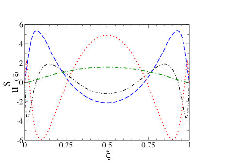
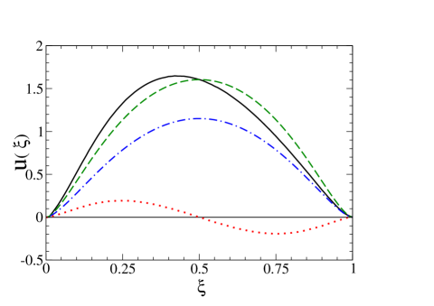
Figure 1: (Color online). Left panel: the symmetric pion PDF, $u^{S}(\xi)$, with its contributions $u^{S}_{N}(\xi)$, $u^{S}_{d}(\xi)$ and $u^{S}_{2d}(\xi)$ (cf Eq. (IV.1)). Dash-dotted line: $u^{S}(\xi)$. Dashed line: $u^{S}_{N}(\xi)$. Dotted line: $u^{S}_{d}(\xi)$. Dash-double-dotted line: $u^{S}_{2d}(\xi)$. Right panel: $u^{q}(\xi)$, $u^{S}(\xi)$, $u^{AS}(\xi)$ and the LF-valence PDF of the pion, $u^{LF}_{val}(\xi)$. Solid line: quark PDF, Eq. (36). Dashed line: $u^{S}(\xi)$. Dotted line: $u^{AS}(\xi)$. Dash-dotted line: $u^{LF}_{val}(\xi)$ (see Ref. [76]), with normalization equal to $P_{val}=0.7$ (see text).

A first consistency check of our formalism has been carried out in Appendix C.1, where it is shown that, within the Mandelstam approach, $f^{S}_{1}(\gamma,\xi)$ and in turn $f^{q}_{1}(\gamma,\xi)$ are normalized to $1$, as naturally follows from the canonical BS-amplitude normalization [80, 92], performed according to Eq. (8) (see also Ref. [62]). In particular, the integral on $\gamma$ and $\xi$ of ${\cal I}_{N}(\gamma,\xi;S)$ saturates the normalization, while the other two terms provide vanishing contributions. Hence, one gets

$$\int_{0}^{1}d\xi\int_{0}^{\infty}d\gamma~{}f^{S}_{1}(\gamma,\xi)$$

$$=\int_{0}^{1}d\xi\int_{0}^{\infty}d\gamma~{}{\cal I}_{N}(\gamma,\xi;S)$$

$$=\int_{0}^{1}d\xi\int_{0}^{\infty}d\gamma~{}f^{q}_{1}(\gamma,\xi)=1.$$ (34)

It should be recalled that all the calculated uTMDs vanish outside the interval $0\leq\xi\leq 1$, as dictated by the conservation of the plus components of the four-momenta of both pion and constituents (cf. Eq. (10)). It is understood that the integral of $f^{AS}_{1}(\gamma,\xi)$ is vanishing, given the antisymmetry with respect to $\xi\to 1-\xi$.

IV.1 Longitudinal degree of freedom

The symmetric and the anti-symmetric PDFs, $u^{S(AS)}(\xi)$ (for the explicit expressions see Appendix D) are defined by

$$u^{S(AS)}(\xi)=\int_{0}^{\infty}d\gamma~{}f^{S(AS)}_{1}(\gamma,\xi)$$ (35)

$$=u^{S(AS)}_{N}(\xi)+u^{S(AS)}_{d}(\xi)+u^{S(AS)}_{2d}(\xi)+u^{S(AS)}_{3d}(\xi)~{},$$

with the normalization that follows from Eq. (34) and the vanishing result of the double integration of $f^{AS}_{1}(\gamma,\xi)$. Finally, the quark and anti-quark PDFs are evaluated through

$$u^{q(\bar{q})}(\xi)=u^{S}(\xi)\pm u^{AS}(\xi)~{},$$ (36)

with the normalization still given by Eq. (34). Within the SU(3)-flavor symmetry, one has to implement the charge symmetry (see, e.g. Ref. [81]) at the initial scale, and therefore $u^{S}(\xi)$ is the PDF to be compared, after the proper evolution, with the experimental data, as it has been shown in Ref. [76].

In the left panel of Fig. 1, $u^{S}(\xi)$ and its three contributions (see Eqs. (111), (112) and (113)) are shown. The calculation has been carried out by adopting the BS-amplitude obtained by using the solution of the BSE as described in Ref. [62], using the following values of the three input parameters: $m=255$ MeV, $\mu=637.5$ MeV and $\Lambda=306$ MeV, able to reproduce the pion decay constant $f^{PDG}_{\pi}=130.50(1)(3)(13)\,$MeV [93] (recall that the pion charge radius results to be $r_{ch}=0.663\,$fm [75], in excellent agreement with $r^{PDG}_{ch}=0.659\pm 0.004\,$fm [94]). A remarkable cancellation among the contributions takes place, and this represents a common feature for all the integrated quantities generated by the uTMDs we are considering. In the right panel, one can see the comparison between the quark PDF, $u^{S(AS)}(\xi)$ and the LF-valence PDF, resulting from the one-to-one relation between the LF-projected BS amplitude and the valence amplitude of the Fock expansion of the pion state. In particular, the LF-valence PDF (see Refs. [62, 76]), is given by

$$u^{LF}_{val}(\xi)=\int_{0}^{\infty}{d\gamma\over(4\pi)^{2}}~{}\Bigl{[}|\psi_{\uparrow\downarrow}(\gamma,z)|^{2}+|\psi_{\uparrow\uparrow}(\gamma,z)|^{2}\Bigr{]}\,,$$ (37)

where $\xi=(1-z)/2$, $\psi_{\uparrow\downarrow}(\gamma,z)$ is the anti-aligned component of the LF-valence amplitude and $\psi_{\uparrow\uparrow}(\gamma,z)$ the aligned one (of purely relativistic nature having an orbital angular momentum equal to $1$). These amplitudes are suitable combinations of the LF-projected scalar functions $\phi_{i}(k;P)$, Eq. (22). The integral on $\xi$ of LF-valence PDF gives the probability of the valence state in the Fock expansion and amounts to

$$P_{val}=\int_{0}^{1}d\xi~{}u^{LF}_{val}(\xi)=0.7\,.$$ (38)

The striking feature shown in the left panel is the shift toward low $\xi$ of the quark PDF, so that for this quantity the symmetry $\xi\to 1-\xi$ is slightly violated.

IV.2 Analysing the shift and the gluon content

The PDF calculations based on the BS-amplitude are able to capture an explicit gluonic effect, to be taken distinct from the one responsible for the effective mass of the constituents. In particular, the difference between the two symmetric PDFs, i.e. $u^{S}(\xi)$ and $u^{LF}_{val}(\xi)$ (recall that has $P_{val}=0.7$), can be traced back to the non negligible probability of the higher Fock states (HFS), where a $q\bar{q}$ pair interacts by exchanging any number of gluons. Interestingly, the difference can be effectively described only by a factor, since it turns out that $u^{LF}_{val}(\xi)/P_{val}$ largely overlaps $u^{S}(\xi)$. Finally, also the small, but relevant, shift of the quark PDF with respect to $u^{S}(\xi)$ has to be ascribed to the presence of HFS, as discussed in what follows.

To get a qualitative view, we remind that the pion state can be, in principle, decomposed in Fock-components, which are schematically written in ladder approximation as

$$|\pi\rangle=|q\bar{q}\rangle+|q\bar{q}g\rangle+|q\bar{q}\,2g\rangle+\cdots$$ (39)

Due to the charge symmetry, each Fock-component is invariant by $q\leftrightarrow\bar{q}$, and hence the valence state $|q\bar{q}\rangle$ provides a symmetric contribution to $u^{q}(\xi)$, identified with $u_{val}^{LF}(\xi)$. The following terms contain gluons up to infinity. In our model, the gluon has an effective mass about twice the quark mass, so that the HFS cumulative effect results in a small shift of the $u^{q}(\xi)$ peak at $\xi<1/2$, as shown in the right panel of Fig. 1. Actually, a similar effect, related to the increasing mass of the remnant, can be also recognized in the nucleon, where one has a valence parton distribution with a peak around 1/3 due to the presence of the other two constituent quarks. In the case of the pion, the effect is small since the valence component $|q\bar{q}\rangle$ has 70% of probability (as generated by our dynamical calculation), and hence is largely dominant.

To become more quantitative and illustrate this effect, we schematically write the quark PDF by using the Fock expansion of the pion state, Eq. (39), and inserting LF variables [79], one has

$$u^{q}(\xi)=\sum_{n=2}^{\infty}\,\Bigg{\{}\prod_{i}^{n}\int\frac{d^{2}k_{i\perp}}{(2\pi)^{2}}\int^{1}_{0}d\xi_{i}\Bigg{\}}\,$$

$$\times\delta\left(\xi-\xi_{1}\right)\delta\left(1-\sum_{i=1}^{n}\xi_{i}\right)\,\delta\left(\sum_{i=1}^{n}{\bf k}_{i\perp}\right)$$

$$\times\big{|}\Psi_{n}(\xi_{1},{\bf k}_{1\perp},\xi_{2},{\bf k}_{2\perp},...)\big{|}^{2}\,,$$ (40)

where $\xi_{1(2)}$ is the longitudinal-momentum fraction of the quark (antiquark) in each Fock state, composed by a $q\bar{q}$ pair and $n-2$ gluons, generated by the iteration of the one-gluon exchange. Moreover, $\Psi_{n}(\xi_{1},{\bf k}_{1\perp},\xi_{2},{\bf k}_{2\perp},...)$ is the probability amplitude of the corresponding Fock component and fulfills a normalization condition that follows from the one of the pion state. In the $n$-th state one has

$$\xi_{1}=1-\xi_{2}-\sum_{g=3}^{n}\xi_{g}~{}~{}.$$ (41)

Since $\xi_{i}>0$ for massive particles, the average value of $\xi_{1}$ starts to decreases while the number of gluons increases, as quantitatively shown in what follows.

Looking at the right panel of Fig. 1, one can realize that while the valence term, with probability $P_{val}=0.7$, has a peak at $\xi_{1}=\xi_{2}=1/2$, given the symmetry of $|\Psi_{2}(\xi_{1},{\bf k}_{1\perp},\xi_{2},{\bf k}_{2\perp})|^{2}$ all the HFS shift the peak to $\xi_{1}<1/2$, and decrease the tail, due to the constraint of the overall normalization. This is reflected in the evaluation of the first moment (recall $\xi_{q}\equiv\xi_{1}$)

$$\langle\xi_{q}\rangle=P_{val}~{}\langle\xi_{q}\rangle_{val}+\sum_{n>2}P_{n}~{}\langle\xi_{q}\rangle_{n}$$

$$=P_{val}~{}\langle\xi_{q}\rangle_{val}+(1-P_{val})~{}\langle\xi_{q}\rangle_{HFS}~{},$$ (42)

where $P_{n}$ is the probability of the $n$-th Fock state beyond the valence one. The first term in Eq. (42) is equal to $0.35$, since $1/2$ is weighted by $P_{val}$, and the rest is weighted by $0.3$. Notice that for each HFS, normalized to 1, one has

$$\langle\xi_{q}\rangle_{n} = 1-\langle\xi_{\bar{q}}\rangle_{n}-\sum_{i=3}^{n}\langle\xi_{g_{i}}\rangle_{n}$$ (43)

$$= 1-\langle\xi_{\bar{q}}\rangle_{n}-(n-2)\langle\xi_{g}\rangle_{n}\,,$$

where the gluon bosonic nature leads to the factor $n-2$.

The actual value of the first moment of $u^{q}(\xi)$ is

$$\langle\xi_{q}\rangle=\int_{0}^{1}d\xi\int_{0}^{\infty}d\gamma~{}\xi~{}f^{q}_{1}(\gamma,\xi)=0.471~{},$$ (44)

that amounts to an average of $\langle\xi_{q}\rangle_{HFS}$ equal to $0.40$.

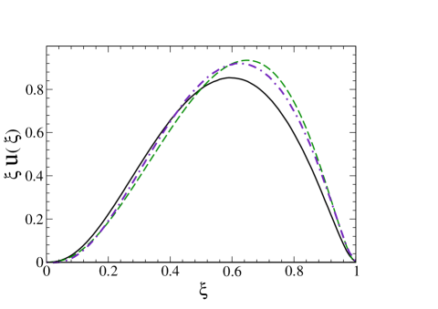
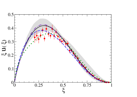
Figure 2: (Color online). Left panel. Pion longitudinal distributions, with different scales (see text for details). Dashed line: $\xi\,u^{S}(\xi)$, with an assigned initial scale equal to $360\,$MeV, and first moment equal to $0.5$. Solid line: $\xi\,u^{q}(\xi)$, with a deduced scale equal $389\,$MeV, obtained by using a backward evolution of the first moment $\langle\xi_{q}\rangle=0.471$. Dot-dashed line $\xi~{}u^{q}(\xi)$ backward-evolved from $389\,$MeV to $360\,$MeV. Right panel. Comparison with the experimental data at the scale $5.2\,$GeV. Solid line: evolved $u^{S}(\xi)$ starting from $360\,$MeV. Dot-dashed line: evolved $u^{q}(\xi)$, starting from $389\,$MeV. Dashed line: DSE calculation from Fig. 5 of Ref. [95]. Dotted line: BLFQ result at $4.0$ GeV [96]. Shaded area: LQCD calculation extracted via Mellin moments from Ref. [97]. Full squares: reanalyzed data by using the ratio between the fit 3 of Ref. [98], evolved to $5.2\,$GeV, and the experimental data [52], at each data point (see Ref. [76] for details).

We can further analyse $\langle\xi_{q}\rangle_{HFS}$, aiming at extracting a quantitative estimate of the exchanged-gluon contribution, $\langle\xi_{g}\rangle$. From the momentum sum rule Eq. (42), and recalling Eq. (41), we get

$$\langle\xi_{q}\rangle_{HFS} = {1\over 1-P_{val}}\sum_{n>2}P_{n}~{}\langle\xi_{q}\rangle_{n}$$ (45)

$$= 1-\langle\xi_{\bar{q}}\rangle_{HFS}-\langle\xi_{g}\rangle\,,$$

where

$$\langle\xi_{g}\rangle={1\over 1-P_{val}}\sum_{n\geq 3}P_{n}(n-2)~{}\langle\xi_{g}\rangle_{n}~{}.$$ (46)

Moreover, since each Fock component fulfills the charge symmetry, i.e. $q\leftrightarrow\bar{q}$, the corresponding quark and antiquark momentum densities are equal and hence for the Mellin moments one has $\langle\xi_{q}^{k}\rangle_{HFS}=\langle\xi_{\bar{q}}^{k}\rangle_{HFS}$ (this property does not imply the charge symmetry of the total density, given the presence of the gluon contribution, cf. Eq. (42)). From Eq. (45), it follows that the gluon contribution reads

$$\langle\xi_{g}\rangle=1-2~{}\langle\xi_{q}\rangle_{HFS}\,.$$ (47)

Then, in our model one has $\langle\xi_{g}\rangle=0.2$. We should note that i) $\langle\xi_{q}\rangle>\langle\xi_{q}\rangle_{HFS}$, as it should be, and ii) the massive gluons carry 20% of the HFS momentum fraction and contribute to the total longitudinal fraction by 6% (recalling that $P_{HFS}=0.3$). This result indicates that the exchanged gluons in the pion are not soft (differently from the ones considered in Ref. [99] where the subtraction of the effect due to soft gluons is advocated for getting a symmetric PDF from the LF projected BS amplitude).

It has to be emphasized that the above analysis, made transparent by the adopted LF variables, is valid in any gauge (both covariant gauges or the light-cone one), and the only difference is the amount of the shift one gets. The possibility to regain the full gauge-invariance by taking into account the additional gluon exchanges that could affect the interaction between the knocked-out quark and the spectator one (see, e.g., the analysis of the gauge-invariance and the hand-bag contribution in Ref. [100, 14]) will be explored elsewhere.

The real test of the longitudinal dof is obviously the comparison between the PDF and the experimental data [52]. As it is shown in Ref. [76], after evolving $u^{S}(\xi)$ from an assigned initial scale of $360\,$ MeV (suggested by the inflection point of the effective running charge $\alpha_{s}(Q^{2})$) to the scale of $5.2\,$GeV, as given by the reanalysis in Ref. [101], the result compares very satisfactorily with the experimental data extracted by taking into account logarithmic resummation effects in the hard part of the Drell-Yan cross-section, as performed in Ref. [98]. Moreover, we have achieved a nice agreement with other dynamical calculations, such as the Dyson-Schwinger result of Ref. [95], the basis light-front quantization calculation of Refs. [102, 103], and also the recent LQCD outcomes of Ref. [97]. In particular, both the overall shape and, importantly, the tail for $\xi\to 1$, gives great confidence in our formalism, and encourages the further steps we have undertaken in this work.

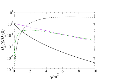
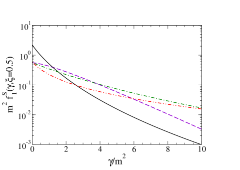
Figure 3: (Color online) Left panel. Normalized pion transverse distribution function, Eq. (48), vs $\gamma/m^{2}$. The normalization is given by $D_{\perp}(0)=22.945\,{\rm GeV^{-2}}$. Thick solid line: full calculation. Dashed line: the same as the full line, but times $(\gamma/m^{2})^{4}$. Dash-dotted line: the same as the full line, but times $(\gamma/m^{2})^{2}$. Dash-double-dotted line: exponential form $e^{-\gamma/(m~{}0.42)^{2}}$, with the parameter from Table 1 of Ref. [35], corresponding to a Gaussian Ansatz for $f_{1}(\gamma,\xi)$ (see text). Right Panel. Pion unpolarized transverse-momentum distribution $f^{S}_{1}(\gamma,\xi)$, Eq. (10), for $\xi=0.5$. Solid line: full calculation as in Fig. 4. Dashed line: LF constituent quark model [56, 35]. Dash-dotted line: LF wave function from DSE calculations [45]. Dash-Double-dotted line: NJL model [38]. The adopted quark mass $m=255\,$MeV.

In Fig. 2, one can observe a further comparison, involving the product $\xi\,u(\xi)$, that sheds more light on the link between the shift of the peak and the gluon dynamics taken explicitly into account in the ladder kernel of the BSE. In particular, we get a scale of $389$ MeV for $u^{q}(\xi)$, the solid line in the left panel of Fig. 1, by backward-evolving its first moment, $\langle\xi_{q}\rangle=0.471$ (cf. Eq. (44)), to $0.5$, the first moment of $u^{S}(\xi)$, that has an assigned hadronic scale of $360$ MeV, as above mentioned and thoroughly discussed in Ref. [76]. In the right panel, the comparison at 360 MeV between $\xi\,u^{S}(\xi)$ and the backward-evolved $\xi\,u^{q}(\xi)$ shows that the effect of the interaction taken into account in the ladder BSE is reproduced at large extent by applying a leading-order DGLAP evolution with an effective running charge as suggested in Ref. [104] and already applied to our PDF in Ref. [76]. This is not surprising once we remind that the dressing of the quark-gluon vertex, as expressed by the effective charge, is governed by the same interaction kernel present in the BSE (i.e. the $q\bar{q}$ amputated T-matrix). The left panel shows the comparison at $5.2\,$GeV between the evolved $u^{S}(\xi)$, starting from the scale of $360\,$MeV, and the evolved $u^{q}(\xi)$, starting from the scale of $389\,$MeV. Nicely, the difference is even smaller.

IV.3 Transverse degree of freedom

In the left panel of Fig. 3, it is shown the transverse distribution defined by

$${\cal D}_{\perp}(\gamma)=\int_{0}^{1}d\xi~{}f^{S}_{1}(\gamma,\xi)=\int_{0}^{1}d\xi~{}f^{q}_{1}(\gamma,\xi)~{}.$$ (48)

It has to be pointed out that the integration on $\xi$ eliminates the anti-symmetric term $f^{AS}_{1}(\gamma,\xi)$, and therefore one gets the same transverse distribution also by using $f^{q}_{1}(\gamma,\xi)$. In order to emphasize the analysis of the general pattern, we have presented ${\cal D}_{\perp}(\gamma)/{\cal D}_{\perp}(0)$, so that the widely adopted exponential or power-like fall-off can be readily compared to our result.

In addition, in the left panel of Fig. 3 one can find: i) an exponential form ${\cal D}_{\perp}(\gamma)/{\cal D}_{\perp}(0)=e^{-\gamma/(m\,0.42)^{2}}$, with the parameter given in Table 1 of Ref. [35], corresponding to the so-called Gaussian Ansätz (recall $\gamma=|{\bf k}_{\perp}|^{2}$), amounting to a factorized form for $f^{S}_{1}(\gamma,\xi)\sim u^{S}(\xi)e^{-\gamma/(0.42^{2})}$ very often adopted in phenomenological studies; ii) our full results multiplied by $(\gamma/m^{2})^{2}$ and iii) our full results multiplied by $(\gamma/m^{2})^{4}$. Not surprisingly, a power-like shape provides a better approximation to the dynamically calculated $D_{\perp}(\gamma)$, but the proper power is different from the one expected by the action of only a one-gluon exchange, that should govern the ultraviolet behavior and lead to a $(\gamma/m^{2})^{2}$ (as suggested by a generalized counting rule in Ref. [105]). Indeed, the adopted form-factor featuring the extension of the quark-gluon interaction vertex (cf. Eq. (7)) generates a different power-like fall-off, namely $(\gamma/m^{2})^{4}$, as already pointed out in Refs. [88, 89]. Finally, it is worth noticing that, unlike the PDF, the two terms in $f^{S}_{1}(\gamma,\xi)$ containing derivatives of the delta-function do not contribute, as it is discussed at the end of Appendix C.1.

In the right panel of Fig. 3, it is presented the quantitative comparison between $f^{S}_{1}(\gamma,\xi)$ at $\xi=0.5$ and some phenomenological outcomes from i) the approach based on the LF wave function obtained by using the DSE calculation in Ref. [45]; ii) the LF constituent quark-model of Ref. [56, 35]; iii) the NJL model with Pauli-Villars regulator as given in Ref. [38]. For $\gamma/m^{2}\to 0$, there are remarkable differences that, indeed, are present also on the tails. This last feature impacts the value of $\langle\gamma/m^{2}\rangle^{\frac{1}{2}}$, as shown in Table 1, where, for the sake of completeness, the value of $u^{S}(\xi=0.5)$ and the pion charge radius are also presented. As can be expected, the larger the average transverse moment, the smaller the radius of charge. The current model has the smaller $\langle\gamma/m^{2}\rangle^{\frac{1}{2}}$ (of the order of the infrared scale $\Lambda_{QCD}$, effectively incorporated in the QCD-inspired choice of our parameters) which in turn leads to a larger charge radius, in agreement with the experimental value.

Table 1: The average value $\langle\gamma/m^{2}\rangle$ (with $m=0.255\,$MeV), $u^{S}(\xi=0.5)$ and the pion charge radius are presented for: i) $f^{S}_{1}(\gamma,\xi=0.5)$ from the present approach (NIR+BSE); ii) the outcome from the LF wave function obtained by using DSE calculation [45] (LFDSE); iii) the LF constituent quark-model of Ref. [56, 35] (LFCQM) and iv) the NJL with Pauli-Villars regulator [38]. (Recall that the most recent PDG value of the charge radius is $r^{PDG}_{ch}=0.659\pm 0.004$ fm [94]).

	$\langle\gamma/m^{2}\rangle^{\frac{1}{2}}$	$u^{S}(\xi=0.5)$	$r_{ch}$ [fm]
NIR+BSE	1.25	1.60	0.663
LFDSE	1.94	1.36	0.590
LFCQM	1.65	1.37	0.572
NJL	2.02	1.01	0.557

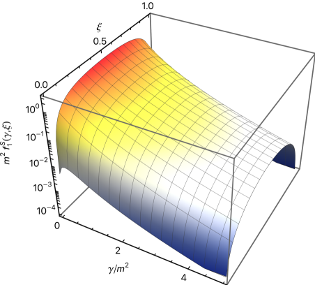
Figure 4: (Color online) Pion unpolarized transverse-momentum distribution $f^{S}_{1}(\gamma,\xi)$, Eq. (10), at the initial scale. The normalization is $\int_{0}^{1}d\xi\int_{0}^{\infty}d\gamma~{}f^{S}_{1}(\gamma,\xi)=1$.

In Fig. 4, the uTMD $f^{S}_{1}(\gamma,\xi)$ is shown in full, in order to appreciate the main features, i.e. i) the peak at $\xi=0.5$ for running $\gamma/m^{2}$, ii) the vanishing values at the end-points and iii) the order of magnitude fall-off already for $\gamma/m^{2}>2$. Comparing to other approaches, one can notice the sharp difference with the results from the LF constituent model in Ref. [56] and the LF holographic framework, like in Refs. [57, 40] where a double-humped structure is found due to the $\xi$-dependence in the holographic wave functions. Also the value at $\xi=0.5$ and small $\gamma/m^{2}$ is substantially lower than ours (almost an order of magnitude less). Differently, the shape of our $f^{S}_{1}(\gamma,\xi)$ is more similar, i.e. without any double-humped structure, to the one obtained in Ref. [45], where the pion LF-wave function is determined from a beyond rainbow-ladder Dyson-Schwinger equations (DSE) in Euclidean space, by exploiting the $\gamma$-dependent moments in $\xi$ and a suitable parametrization of the BS-amplitude.

V The subleading-twist uTMDs

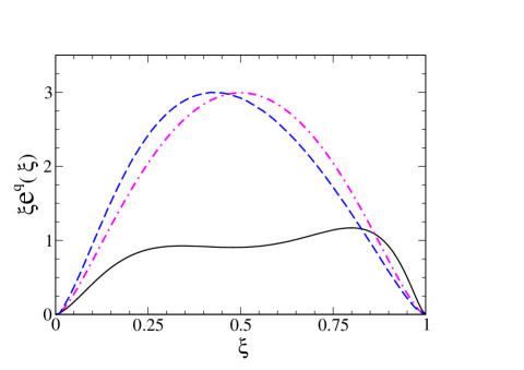
Figure 5: (Color online) Left panel. Pion unpolarized collinear PDFs: i) $e^{q}(\xi)$ (solid line), Eq. (51), ii) $e^{S}(\xi)$ (dashed line) and $e^{AS}(\xi)$ (dotted line), Eqs. (50). It is also shown $e^{q}_{EoM}(\xi)$ (dash-dotted line), Eq. (52). Right panel. Quark unpolarized collinear PDFs: $\xi~{}e^{q}(\xi)$. Solid line: full calculation as in the left panel. Dashed line: $m/M~{}u^{q}(\xi)$, with $u^{q}(\xi)$ shown in the right panel of Fig. 1. Double-dot-dashed line: $\xi~{}e^{q}_{EoM}(\xi)$, Eq. (52).

In this Section we present the numerical results for (T-even) uTMDs beyond the leading-twist. The detailed expressions can be found in the Appendix E, but it is useful to recall that the decomposition in symmetric and antisymmetric combinations adopted for $f_{1}(\gamma,\xi)$ remains still valid, as well as the relations with the quark and anti-quark contributions.

As introduction to the outcomes of our dynamical approach, it is worth anticipating that the comparison between full calculations and naive estimates one can infer from Eq. (17) by using a valence approximation of the leading-twist $f_{1}(\gamma,\xi)$, highlights the inspiring statement one can read in Ref. [77]: the higher-twist distributions are naturally related to multiparton distributions. The role of the exchanged gluons becomes definitely clear through a remarkable shift of the peak in all the sub-leading uTMD we have analyzed, as already discussed in the previous Section, as well as through the sharp difference with the naive estimates, which exclude the effect of the one-gluon exchange.

V.1 Twist-3 uTMD: $e(\gamma,\xi)$

In the frame where ${\bf P}_{\perp}=0$ and hence $P^{+}=M$, by using Eq. (32), (85), (86), (87) and (88), with $i=1$ and the functions $b^{1}_{n;\ell j}$ given in Table 7, one gets the twist-3 uTMDs $e^{S(AS)}(\gamma,\xi)$, decomposed as follows

$$e^{S(AS)}(\gamma,\xi)={\cal E}_{0}(\gamma,\xi;S(AS))+{\cal E}_{d}(\gamma,\xi;S(AS))$$

$$+{\cal E}_{2d}(\gamma,\xi;S(AS))+{\cal E}_{3d}(\gamma,\xi;S(AS))~{},$$ (49)

where the functions in the rhs are given in Appendix E.

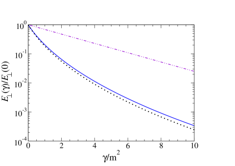
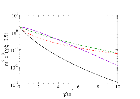
Figure 6: (Color online). Left panel. Normalized transverse distribution function $E_{\perp}(\gamma)/E_{\perp}(0)$ (cf. Eq. (54)). Dotted line: full calculation. Solid line: $D_{\perp}(\gamma)/D_{\perp}(0)$ for the sake of comparison. Dash-double-dotted line: the same as in the left panel of Fig. 3. Right panel. Pion unpolarized transverse-momentum distribution $e^{S}(\gamma,\xi)$, Eq. (49), for $\xi=0.5$. Solid line: full calculation. Dashed line: LF constituent quark model of Ref. [56, 35], but multiplied by $m/(M~{}0.5)$ (cf. Eq. (52)). Dash-dotted line: the same as the dashed line but with the LF wave function from DSE calculations [45]. Dash-Double-dotted line: the same as the dashed line but with the NJL model [38]. The adopted quark mass $m=255\,$MeV.

V.1.1 Longitudinal degree of freedom

In the left panel of Fig. 5, the following collinear PDFs are shown

$$e^{(S,AS)}(\xi)=\int_{0}^{\infty}d\gamma~{}e^{(S,AS)}(\gamma,\xi)~{}.$$ (50)

and

$$e^{q}(\xi)=e^{S}(\xi)+e^{AS}(\xi)~{}.$$ (51)

Moreover, in the spirit of Ref. [35], we also present the collinear PDF, $e^{q}_{EoM}(\xi)$, obtained by integrating the first line in Eq. (17), but disregarding the gluon contribution, viz

$$e^{q}_{EoM}(\xi)\sim{m\over M\xi}\int_{0}^{\infty}d\gamma~{}f^{q}_{1;EoM}(\gamma,\xi)$$

$$\sim{m\over M\xi}~{}{u^{LF}_{val}(\xi)\over P_{val}}~{},$$ (52)

where $u^{LF}_{val}(\xi)/P_{val}$, normalized to $1$ (cf. Eq. (38)), approximates the integral of $f^{q}_{1;EoM}(\gamma,\xi)$. The large difference between our $e^{q}(\xi)$ and $(m/M\xi)u^{LF}_{val}(\xi)/P_{val}$ indicates the sizable role of the gluon contribution from the HFS generated by our dynamical model. In addition, one should point out that the strength of $e^{q}(\xi)$ is spread out on the whole range of $\xi$, and not concentrated at the end-point $\xi=0$ as QCD investigations indicate. The latter feature leads to the singular contribution given in Eq. (15) (see, e.g., Ref. [85], for a detailed discussion, but notice that the focus is on the nucleon).

In the right panel of Fig. 5, the comparison between $\xi\,e(\xi)$ and the other two approximations: i) $(m/M)f^{q}_{1}(\xi)$ and ii) $(m/M)u^{LF}_{val}(\xi)$ (cf. Eq. (52)) is carried out. The relevance of such a comparison is given by the possibility of more directly assessing the gluon role, since the factor $\xi$ eliminates the singular term present in the QCD analysis of $e(\xi)$, and one remains with the mass contribution $(m/M)f^{q}_{1}(\xi)$ and the term from the quark-gluon-antiquark correlator.

Still within the QCD framework (see, e.g., Ref. [85]), the moments $\langle\xi^{n}\rangle_{e^{q}}$, for $n\leq 2$, read as follow

$$\int d\xi~{}e^{q}(\xi)={\sigma_{\pi}\over m_{cur}}$$

$$\int d\xi~{}\xi~{}e^{q}(\xi)={m_{cur}\over M}$$

$$\int d\xi~{}\xi^{2}~{}e^{q}(\xi)={m_{cur}\over M}\int d\xi~{}\xi~{}f^{q}_{1}(\xi)~{},$$ (53)

and, for $n>2$, they receive contributions not only from the $(n-1)$-th moment of $f^{q}_{1}(\gamma,\xi)$ , but also from the $n$-th moment of the twist-3 contribution pertaining to the quark-gluon-antiquark correlator. Given the highly non trivial dynamical content of the $e^{q}(\xi)$ moments, it is interesting to show the results obtained with our dynamical model.

Table 2: The moments $\langle\xi^{n}\rangle_{e^{q}}$ of the quark twist-3 $e^{q}(\gamma,\xi)$ for $n<4$, and the ratio $R(n,e^{q},f^{q}_{1})=\langle\xi^{n}\rangle_{e^{q}}/\langle\xi^{n-1}\rangle_{f^{q}_{1}}$ (it is assumed $\langle\xi^{-1}\rangle_{f^{q}_{1}}=\langle\xi^{0}\rangle_{f^{q}_{1}}=1$, and the values of $\langle\xi^{1}\rangle_{f^{q}_{1}}=0.471$ and $\langle\xi^{2}\rangle_{f^{q}_{1}}=0.266$ have been numerically evaluated).

$n$	0	1	2	3
$\langle\xi^{n}\rangle_{e^{q}}$	2.190	0.814	0.445	0.292
$R(n,e^{q},f^{q}_{1})$	2.190	0.814	0.943	1.10

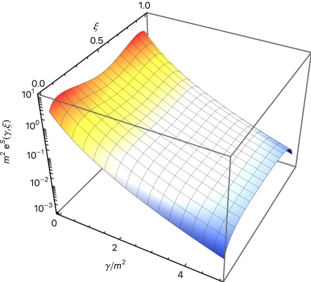
Figure 7: (Color online) Pion unpolarized transverse-momentum distribution $e^{S}(\gamma,\xi)$, Eq. (50), at the initial scale.

In Table 2, both the moments up to $n=3$ and the ratio $R(n,e^{q},f^{q}_{1})=\langle\xi^{n}\rangle_{e^{q}}/\langle\xi^{n-1}\rangle_{f^{q}_{1}}$ are presented. In particular, as to the first two moments, to get rid of the dependence upon $m_{cur}$ it is helpful to compare the result obtained by multiplying the zero-th and the first moment, (cf. Eq. (53)), with final outcome $\sigma_{\pi}/M$. The estimate of $\sigma_{\pi}$ at the leading order of the chiral expansion leads to $\sigma_{\pi}/M=1/2$, as satisfactorily confirmed by the lattice calculations in Ref. [84], where $\sigma^{lat}_{\pi}=78.2\pm 4.2\,$MeV, for $M=149.5\pm 1.3\,$MeV and $m_{cur}\sim 4.9\,$MeV. Eliminating the current quark mass, that is outside our approach, through the above product, we get $\sigma_{\pi}/M=1.78$, instead of $\sim 0.5$. Such a conspicuous difference is surely influenced by the different distribution of the $e^{q}(\xi)$ strength, as already mentioned, and points to a needed enrichment of the gluon dynamics in our approach. However, it is worth mentioning that for a simple non relativistic constituent quark model one has $\sigma_{\pi}^{NR}=2m$, so that $\sigma_{\pi}^{NR}/M=3.64$ (with $m=255$ MeV the constituent mass), almost twice the result obtained in the BS framework.

In QCD, the ratios $R(1,e^{q},f^{q}_{1})$ and $R(2,e^{q},f^{q}_{1})$ are equal and amount to $m_{cur}/M$ (see Eq. (53)), while $R(3,e^{q},f^{q}_{1})=m_{cur}/M+\Delta^{3}_{g}$, where $\Delta^{3}_{g}$ contains the contribution from the twist-3 gluonic contribution. In our calculation, the ratios for $n=1,2$ are almost equal, but different from the naive expectation $m/M=1.82$ with the adopted $m=255$ MeV. The difference with the third ratio indicates the onset of the contribution from the twist-3 gluonic term.

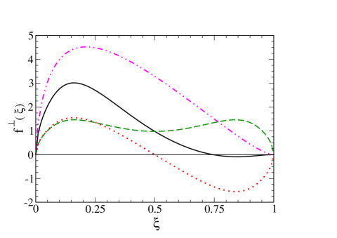
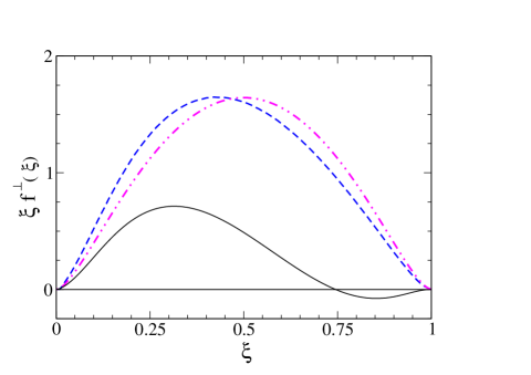
Figure 8: (Color online) Left panel. The same as in Fig. 5, but for $f^{\perp q}(\xi)$, $f^{\perp S}(\xi)$ and $f^{\perp AS}(\xi)$, Eq. (56), and $f^{\perp q}_{EoM}(\xi)$ as given in Eq. (57). Right panel. Quark unpolarized collinear PDFs $\xi\,f^{q\perp}(\xi)$. Solid line: full calculation as in left panel. Dashed line: $\xi\,f^{q\perp}(\xi)$ obtained by using the second line in Eq. (17) and our $f^{q}_{1}(\xi)$. Double-dot-dashed line: the same as the dashed line but using the valence approximation of the PDF, $u^{LF}_{val}(\xi)$, with norm equal to $1$.

V.1.2 Transverse degree of freedom

The transverse dof can be analyzed globally by introducing the following transverse distribution function, as already accomplished with the leading-twist uTMD, viz.

$$E_{\perp}(\gamma)=\int_{0}^{1}d\xi~{}e^{S}(\gamma,\xi)=\int_{0}^{1}d\xi~{}e^{q}(\gamma,\xi)~{}.$$ (54)

In the left panel of Fig. 6, it is presented our calculation and the ratio $D_{\perp}(\gamma)/D_{\perp}(0)$ to show the similar fall-off, as generated from gluon dynamics and the form-factor featuring the quark-gluon vertex.

A more close view of the decreasing as a function of $\gamma/m^{2}$ is provided by the right panel of Fig. 6, where it is shown the comparison between our calculation of $e(\gamma,\xi=0.5)$ and the outcomes obtained by using Eq. (52) with i) the LF wave function from the constituent quark model of Ref. [56, 35], ii) the LF wave function from DSE calculations [45] and iii) the PDF from the NJL model [38]. The differences again point to the role of the interaction in the various approaches, and highlight the relevance of an experimental investigation of the transverse dof.

In Fig. 7, the full dependence of $e^{S}(\gamma,\xi)$ is presented, displaying a double-hump shape that for larger $\gamma/m^{2}$ becomes smoother and smoother.

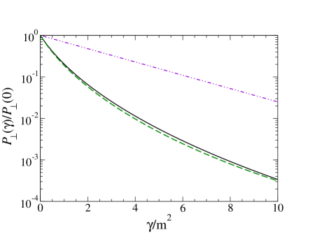
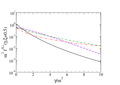
Figure 9: (Color online). Left panel. Normalized transverse distribution function $P_{\perp}(\gamma)/P_{\perp}(0)$ (cf. Eq. (58)). Dotted line: full calculation. Solid line: $D_{\perp}(\gamma)/D_{\perp}(0)$ for the sake of comparison. Dash-double-dotted line: the same as in the left panel of Fig. 3. Right panel. Pion unpolarized transverse-momentum distribution $f^{S\perp}(\gamma,\xi)$, Eq. (55), for $\xi=0.5$. Solid line: full calculation. Dashed line: by using $f_{1}(\gamma,\xi=0.5)$ in Fig. 3 from the LF constituent quark model of Ref. [56, 35] (cf. the second line in Eq. (17), without the gluonic term). Dash-dotted line: the LF wave function from DSE calculations [45]. Dash-Double-dotted line: the NJL model [38]. The adopted quark mass $m=255$ MeV.

V.2 Twist-3 uTMD: $f^{\perp}(\gamma,\xi)$

In an analogous way, for $i=2$ and using Table 8, one gets the twist-3 $f^{\perp S(AS)}(\gamma,\xi)$, with the following decomposition

$$f^{\perp S(AS)}(\gamma,\xi)={\cal P}_{0}(\gamma,\xi;S(AS))+{\cal P}_{d}(\gamma,\xi;S(AS))$$

$$+{\cal P}_{2d}(\gamma,\xi;S(AS))$$ (55)

where the above functions are given in Appendix E. Notice that in this case ${\cal P}_{2d}(\gamma,\xi;S(AS))=0$.

V.2.1 Longitudinal degree of freedom

In the left panel of Fig. 8, the following collinear PDFs are shown

$$f^{\perp S(AS)}(\xi)=\int_{0}^{\infty}d\gamma~{}f^{\perp S(AS)}(\gamma,\xi)~{}~{},$$ (56)

and the corresponding quark combination. As a reference, it is also presented $f^{\perp q}_{EoM}(\xi)$, obtained from the second line of Eq. (17), without the gluon term, as follows

$$f^{\perp q}_{EoM}(\xi)\sim{1\over\xi}\int_{0}^{\infty}d\gamma f^{\perp q}_{EoM}(\gamma,\xi)\sim{u^{LF}_{val}(\xi)\over\xi}~{}.$$ (57)

For the sake of completeness, in the right panel of Fig. 8, the product $\xi\,f^{q\perp}(\xi)$ is compared to $f^{q}_{1}(\xi)$ and $u^{LF}_{val}(\xi)$ that represents the approximation to $f^{\perp q}_{EoM}(\xi)$ as given in Eq. (57). Also for $f^{q\perp}(\xi)$, the full calculation substantially differs from approximated evaluations, prompting further investigation of the gluon contributions.

V.2.2 Transverse degree of freedom

Also for $f^{\perp}(\gamma,\xi)$, we introduce the transverse distribution function, viz.

$$P_{\perp}(\gamma)=\int_{0}^{1}d\xi~{}f^{S\perp}(\gamma,\xi)=\int_{0}^{1}d\xi~{}f^{q\perp}(\gamma,\xi)~{}.$$ (58)

In the left panel of Fig. 9, a comparison, built with the same spirit as in the left panel of Fig. 6, is shown for the ratio $P_{\perp}(\gamma)/P_{\perp}(0)$.

A more detailed view of the fall-off can be gained from the right panel of Fig. 9, where $f^{S\perp}(\gamma,\xi=0.5)$ is compared with the results obtained by using i) the LF constituent quark model of Ref. [56, 35] (cf. the second line in Eq. (17), without the gluonic term). ii) the LF wave function from DSE calculations [45] and iii) the NJL model [38].

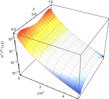
Figure 10: (Color online) Pion unpolarized transverse-momentum distribution $f^{S\perp}(\gamma,\xi)$, Eq. (55).

Finally in Fig. 10, the full dependence of $f^{S\perp}(\gamma,\xi)$ is shown. Also in this uTMD, the double-hump shape decreases when $\gamma/m^{2}$ increases.

To summarize, a coherent view of the tail in $\gamma$ is plainly provided by Figs. 3, 6 and 9. Namely, the interaction taken into account in the ladder kernel together with the extended structure of the quark-gluon vertex governs the fall-off of both the leading and subleading-twist uTMDS. Therefore, the quantitative estimates obtained through our dynamical model, in Minkowski space, is shown to be in a favorable position to provide insights into the interplay between transverse dof and the role of gluons.

VI Conclusions

The twist-2 (leading) and twist-3 (subleading) unpolarized (T-even) transverse-momentum dependent parton distribution functions have been calculated for the pion within an approach based on the solution of the Bethe-Salpeter equation in Minkowski space, namely, within a genuinely relativistic quantum-field theory framework. We achieved this goal by exploiting the Nakanishi integral representation of the BS-amplitude in order to get actual solution of the homogeneous BSE, in ladder approximation, through a system of integral equations that determine the Nakanishi weight functions relevant for the problem under scrutiny [88, 89, 62]. After obtaining the pion electromagnetic form factor [75], and the pion PDF [76], we extended the yield of our approach by exploring the dependence of the parton distributions upon the transverse momentum. This additional step has its-own importance in view of the planned experimental efforts to achieve a fully three-dimensional investigation of hadrons (mainly of the nucleon and, more challenging, the pion).

The relevant message one gets from our calculations is given by the essential role of the gluon exchange, that cannot be captured by purely phenomenological model. The joint use of the Fock expansion of the pion state, allows us to shed light on the gluonic content of the quark PDF obtained through the BS amplitude, even determining a quantitative estimate, $\sim 6\%$ of the average longitudinal momentum fraction $\langle\xi^{q}\rangle$. Moreover, the latter analysis explains also the source of the small, but theoretically relevant, shift between the $u^{q}(\xi)$ and the PDF that fulfills the charge symmetry (an issue already investigated within the Dyson-Schwinger approach, e.g., in Ref. [99], where a different interpretation was proposed). As to the transverse degree of freedom, a power-like fall-off of the transverse distributions, obtained by integrating on $\xi$ the uTMDs, is supported by the one-gluon exchange interaction that governs the ultraviolet region, according to our calculations. This outcome could suggest to reconsider an exponential or Gaussian Ansatzes for describing the high-momentum content ($\gamma>>m^{2}$) of the uTMDS.

Summarizing, our approach can be placed among those in which the dynamics can be studied in Minkowski space and in some detail. Moreover, the additive construction of the interaction kernel allows one to address step-by-step recognized effects, achieving an implementation of the dynamics in a controlled way.

Appendix A Traces

In this Appendix the traces in Eqs. (10), (18) and (19), are explicitly evaluated, presenting the expressions of the functions $a^{i}_{\ell,j}(k^{-},\gamma,z;S(AS))$ and $b^{i}_{n;\ell,j}(\gamma,z;S(AS))$. For the sake of convenience, let us rewrite the generic trace entering Eq. (23)

$$Tr^{S(AS)}_{i}(\gamma,\xi)=-{i\over 2}\left\{\text{Tr}\left[S^{-1}(k-\tfrac{P}{2})\bar{\Phi}(k,P)~{}{\cal O}_{i}~{}\Phi(k,P)\right]+\eta^{S(AS)}_{i}~{}\text{Tr}\left[S^{-1}(k+\tfrac{P}{2})\Phi(k,P)~{}{\cal O}_{i}~{}\bar{\Phi}(k,P)\right]\right\}$$

$$=\sum_{\ell j}~{}a^{i}_{\ell j}(k^{-},\gamma,z;S(AS))~{}\phi_{\ell}(k;P)~{}\phi_{j}(k;P)\,,$$ (59)

with ${\cal O}^{i}$ and $\eta^{S(AS)}_{i}$ given by

$$\begin{array}[]{ll}{\cal O}_{0}=\gamma^{+}~{},&\quad\eta^{S(AS)}_{0}=\mp 1~{},\\ {}&{}\\ {\cal O}_{1}=\mathbb{1}~{},&\quad\eta^{S(AS)}_{1}=\pm 1~{},\\ {}&{}\\ {\cal O}_{2}={M\over|{\bf k}_{\perp}|^{2}}~{}{\bf k}_{\perp}\cdot{\mbox{\boldmath$\gamma$}}_{\perp}~{},&\quad\eta^{S(AS)}_{2}=\pm 1~{}~{}.\end{array}~{}$$ (65)

To proceed one has to insert the expression of the BS-amplitude, Eq. (II.1), and the definitions, Eqs. (7) and (21), in Eq. (59). Then one gets the results shown in Tables 3, 4 and 5, for $a^{i}_{\ell j}(k^{-},\gamma,z;S(AS))$. It is also useful to organize the functions $a^{i}_{\ell j}$ in powers of $k^{-}$ for preparing the integration on such a variable (cfr Appendix B), i.e.

$$a^{i}_{\ell j}(k^{-},\gamma,z;S(AS))=2M\Biggl{[}b^{i}_{0;\ell j}(\gamma,z;S(AS))+b^{i}_{1;\ell j}(\gamma,z;S(AS))~{}{k^{-}\over 2M}+b^{i}_{2;\ell j}(\gamma,z;S(AS))~{}\Biggl{(}{k^{-}\over 2M}\Biggr{)}^{2}$$

$$+b^{i}_{3;\ell j}(\gamma,z;S(AS))~{}\Biggl{(}{k^{-}\over 2M}\Biggr{)}^{3}\Biggr{]}~{}.$$ (66)

In Tables 6, 7 and 8, one can find the expressions for $b^{i}_{n;\ell j}(\gamma,z;S(AS))$

Table 3: Non vanishing coefficients $a^{0}_{\ell j}(k^{-},\gamma,z;S(AS))$.

$~{}ij~{}$	$a^{0}_{\ell j}(S)$		$a^{0}_{\ell j}(AS)$
$11$	$2M$		$2Mz$
$12$	$-8m$
$13$	$-2\,m\,z-4{m\over M}\,k^{-}$
$14$	$-{8\over M}\gamma-M\,z^{2}-2\,z\,k^{-}$		$-Mz-2k^{-}$
$22$	$2M$		$-4k^{-}$
$23$	$M\,z+2\,k^{-}$		$-8{\gamma\over M}-2zk^{-}-{4\over M}(k^{-})^{2}$
$24$			$2mz+4{m\over M}k^{-}$
$33$	${M\over 2}\Bigl{(}4{\gamma\over M^{2}}+{z^{2}\over 4}\Bigr{)}+{z\over 2}k^{-}+{1\over 2M}\,(k^{-})^{2}$		$-\Bigl{(}4{\gamma\over M^{2}}+{z^{2}\over 4}\Bigr{)}k^{-}-{z\over M}(k^{-})^{2}-{1\over M^{2}}(k^{-})^{3}$
$34$			$2m\Bigl{(}4{\gamma\over M^{2}}+{z^{2}\over 4}\Bigr{)}+2{m\over M}zk^{-}+2{m\over M^{2}}(k^{-})^{2}$
$44$	${M\over 2}\Bigl{(}4{\gamma\over M^{2}}+{z^{2}\over 4}\Bigr{)}+{z\over 2}k^{-}+{1\over 2M}\,(k^{-})^{2}$		${M\over 2}~{}z\Bigl{(}4{\gamma\over M^{2}}+{z^{2}\over 4}\Bigr{)}+{z^{2}\over 2}k^{-}+{z\over 2M}(k^{-})^{2}$

Table 4: Non vanishing coefficients $a^{1}_{\ell j}(k^{-},\gamma,z;S(AS))$.

$~{}ij~{}$	$a^{1}_{\ell j}(S)$		$a^{1}_{\ell j}(AS)$
$11$	$-4m$
$12$	$4M$		$2Mz-4k^{-}$
$13$			$-{2M}\Bigl{(}4{\gamma\over M^{2}}+{z^{2}\over 4}\Bigr{)}-2zk^{-}-{2\over M}\,(k^{-})^{2}$
$22$	$-4m$
$24$	$-{2M}\Bigl{(}4{\gamma\over M^{2}}+{z^{2}\over 4}\Bigr{)}-2zk^{-}-{2\over M}\,(k^{-})^{2}$
$33$	$m\Bigl{(}4{\gamma\over M^{2}}+{z^{2}\over 4}\Bigr{)}+z{m\over M}k^{-}+{m\over M^{{2}}}\,(k^{-})^{2}$
$34$	$z{M\over 2}\Bigl{(}4{\gamma\over M^{2}}+{z^{2}\over 4}\Bigr{)}-\Bigl{(}4{\gamma\over M^{2}}-{z^{2}\over 4}\Bigr{)}k^{-}-{z\over 2M}(k^{-})^{2}-{1\over M^{2}}(k^{-})^{3}$		$M\Bigl{(}4{\gamma\over M^{2}}+{z^{2}\over 4}\Bigr{)}+zk^{-}+{1\over M}(k^{-})^{2}$
$44$	$m\Bigl{(}4{\gamma\over M^{2}}+{z^{2}\over 4}\Bigr{)}+z{m\over M}k^{-}+{m\over M^{{2}}}\,(k^{-})^{2}$

Table 5: Non vanishing coefficients $a^{2}_{\ell j}(k^{-},\gamma,z;S(AS))$.

$~{}ij~{}$	$a^{2}_{\ell j}(S)$		$a^{2}_{\ell j}(AS)$
$11$	$-4M$
$13$			$8m$
$14$	$4M$		$2zM$ ${-4k^{-}}$
$22$	$4M$
$23$	$-2Mz+4k^{-}$		$-4\,M$
$24$	$-8m$
$33$	$M\Bigl{(}4{\gamma\over M^{2}}+{z^{2}\over 4}\Bigr{)}+zk^{-}+{1\over M}(k^{-})^{2}$
${44}$	$-M\Bigl{(}4{\gamma\over M^{2}}+{z^{2}\over 4}\Bigr{)}-zk^{-}-{1\over M}(k^{-})^{2}$

Table 6: Non vanishing coefficients $b^{0}_{n;\ell j}(\gamma,z;S(AS))$.

$~{}ij~{}$	$b^{0}_{0;\ell j}(S)$	$b^{0}_{1;\ell j}(S)$	$b^{0}_{2;\ell j}(S)$	$b^{0}_{0;\ell j}(AS)$	$b^{0}_{1;\ell j}(AS)$	$b^{0}_{2;\ell j}(AS)$	$b^{0}_{3;\ell j}(AS)$
$11$	$1$	$0$	$0$	$z$	$0$	$0$	$0$
$12$	$-4m/M$	$0$	$0$	$0$	$0$	$0$	$0$
$13$	$-zm/M$	$-4m/M$	$0$	$0$	$0$	$0$	$0$
$14$	$-4{\gamma/M^{2}}-{z^{2}/2}$	$-2\,z$	$0$	$-z/2$	$-2$	$0$	$0$
$22$	$1$	$0$	$0$	$0$	$-4$	$0$	$0$
$23$	${z/2}$	$2$	$0$	$-4\gamma/M^{2}$	$-2z$	$-8$	$0$
$24$	$0$	$0$	$0$	$zm/M$	$4m/M$	$0$	$0$
$33$	${\gamma/M^{2}}+{z^{2}/16}$	${z/2}$	$1$	$0$	$-\Bigl{(}4\gamma/M^{2}+z^{2}/4\Bigr{)}$	$-2z$	$-4$
$34$	$0$	$0$	$0$	$\left(m/{{M}}\right)\Bigl{(}4\gamma/M^{2}+z^{2}/4\Bigr{)}$	$2zm/M$	$4m/M$	$0$
$44$	${\gamma/M^{2}}+{z^{2}/16}$	${z/2}$	$1$	$(z/4)\Bigl{(}4\gamma/M^{2}+z^{2}/4\Bigr{)}$	$z^{2}/2$	$z$	$0$

Table 7: Non vanishing coefficients $b^{1}_{n;\ell j}(\gamma,z;S(AS))$.

$~{}ij~{}$	$b^{1}_{0;\ell j}(S)$	$b^{1}_{1;\ell j}$(S)	$b^{1}_{2;\ell j}(S)$	$b^{1}_{3;\ell j}(S)$	$b^{1}_{0;\ell j}(AS)$	$b^{1}_{1;\ell j}(AS)$	$b^{1}_{2;\ell j}(AS)$
$11$	$-2m/M$	$0$	$0$	$0$	$0$	$0$	$0$
$12$	$2$	$0$	$0$	$0$	$z$	$-4$	$0$
$13$	$0$	$0$	$0$	$0$	$-4{\gamma/M^{2}}-{z^{2}/4}$	$-2z$	$-4$
$22$	$-2m/M$	$0$	$0$	$0$	$0$	$0$	$0$
$24$	$-\Bigl{(}4\gamma/M^{2}+z^{2}/4\Bigr{)}$	$-2z$	$-4$	$0$	$0$	$0$	$0$
$33$	$(m/2M)~{}\Bigl{(}4\gamma/M^{2}+z^{2}/4\Bigr{)}$	$zm/M$	$2m/M$	$0$	$0$	$0$	$0$
$34$	$(z/4)\-\Bigl{(}4\gamma/M^{2}+z^{2}/4\Bigr{)}$	$-\Bigl{(}4\gamma/M^{2}-z^{2}/4\Bigr{)}$	$-z$	$-4$	$2{\gamma/M^{2}}+{z^{2}/8}$	$z$	$2$
$44$	$(m/2M)~{}\Bigl{(}4\gamma/M^{2}+z^{2}/4\Bigr{)}$	$zm/M$	$2m/M$	$0$	$0$	$0$	$0$

Table 8: Non vanishing coefficients $b^{2}_{n;\ell j}(\gamma,z;S(AS))$.

$~{}ij~{}$	$b^{2}_{0;\ell j}(S)$	$b^{2}_{1;\ell j}(S)$	$b^{2}_{2;\ell j}(S)$	$b^{2}_{0;\ell j}(AS)$	$b^{{2}}_{1;\ell j}(AS)$
$11$	$-2$	$0$	$0$	$0$	$0$
$13$	$0$	$0$	$0$	$4(m/M)$	$0$
$14$	$2$	$0$	$0$	$z$	${-4}$
${22}$	${2}$	$0$	$0$	$0$	$0$
$23$	$-z$	$4$	$0$	$-2$	$0$
$24$	$-4m/M$	$0$	$0$	$0$	$0$
$33$	$(1/2)\Bigl{(}4\gamma/M^{2}+z^{2}/4\Bigr{)}$	$z$	$2$	$0$	$0$
$44$	$-(1/2)\Bigl{(}4\gamma/M^{2}+z^{2}/4\Bigr{)}$	$-z$	$-2$	$0$	$0$

Appendix B The light-front projection

The Appendix is devoted to the integration over the variable $k^{-}$ in Eq. (31), that for the sake of clarity we rewrite

$$F^{i}_{\ell j}(\gamma,z;S(AS))=\int_{-\infty}^{\infty}{dk^{-}\over 2\pi}~{}a^{i}_{\ell j}(k^{-},\gamma,z;S(AS))~{}\phi_{\ell}(k,P)\,\phi_{j}(k,P)$$

$$=2M\int_{-\infty}^{\infty}{dk^{-}\over 2\pi}~{}\phi_{\ell}(k,P)\,\phi_{j}(k,P)\times\Biggl{[}b^{i}_{0;\ell j}(\gamma,z;S(AS))+b^{i}_{1;\ell j}(\gamma,z;S(AS)){k^{-}\over 2M}+b^{i}_{2;\ell j}(\gamma,z;S(AS))\Biggl{(}{k^{-}\over 2M}\Biggr{)}^{2}$$

$$+b^{i}_{3;\ell j}(\gamma,z;S(AS))\Biggl{(}{k^{-}\over 2M}\Biggr{)}^{3}\Biggr{]}~{},$$ (67)

where the quantities $a^{i}_{\ell j}(k^{-},\gamma,z;S(AS))$ and $b^{i}_{n;\ell j}(\gamma,z;S(AS))$ are given in Appendix A.

The first step (see also Refs. [62, 75, 76]) is to introduce the NIR of $\phi_{\ell}(k,P)$, Eq. (22), and then apply the Feynman parametrization as follows

$$\phi_{\ell}(k,P)\phi_{j}(k,P)=30\int_{0}^{1}dv\int_{-1}^{+1}dz^{\prime}\int_{0}^{\infty}d\gamma^{\prime}\int_{-1}^{+1}dz^{\prime\prime}\int_{0}^{\infty}d\gamma^{\prime\prime}~{}{v^{2}(1-v)^{2}~{}g_{\ell}(\gamma^{\prime},z^{\prime})~{}g_{j}(\gamma^{\prime\prime},z^{\prime\prime})\over\Bigl{[}k^{-}\alpha-\beta+i\epsilon\Bigr{]}^{6}}~{},$$ (68)

where

$$\alpha={M\over 2}~{}\Bigl{[}\lambda(v)-z\Bigr{]}~{},$$

$$\beta(z\lambda(v))=\gamma+\kappa^{2}+{M^{2}\over 4}z\lambda(v)+v\gamma^{\prime}+(1-v)\gamma^{\prime\prime}~{},$$

$$\lambda(v)=vz^{\prime}+(1-v)z^{\prime\prime}~{}.$$ (69)

Hence, the following general expression, one can straightforwardly deduce from well-known result in Ref. [106] (corresponding to the case $m=0$) is useful for performing the relevant integrals

$$\int_{-\infty}^{\infty}{dk^{-}\over 2\pi}~{}{(k^{-})^{m}\over\Bigl{[}\alpha~{}k^{-}-\beta+i\epsilon\Bigr{]}^{n}}=i~{}{(n-m-2)!\over(n-1)!}{(-1)^{m+1}\over\Bigl{[}-\beta+i\epsilon\Bigr{]}^{n-m-1}}~{}\delta^{(m)}(\alpha)$$ (70)

where $\delta^{(m)}(\alpha)=\partial^{m}\delta(\alpha)/\partial\alpha^{m}$. Finally, combining the results in Eqs. (68) and (70), one gets

$$F^{i}_{\ell j}(\gamma,z;S(AS))=-{24i}\int_{0}^{1}dv~{}v^{2}(1-v)^{2}\int_{-1}^{+1}dz^{\prime}\int_{0}^{\infty}d\gamma^{\prime}\int_{-1}^{+1}dz^{\prime\prime}\int_{0}^{\infty}d\gamma^{\prime\prime}~{}{\cal G}_{\ell j}(\gamma^{\prime},z^{\prime};\gamma^{\prime\prime},z^{\prime\prime};\kappa^{2})$$

$$\times\Biggl{\{}{b^{i}_{0;\ell j}(\gamma,z;S(AS))~{}\delta(\tilde{\alpha})\over[-\beta(z\lambda(v))+i\epsilon]^{5}}-{1\over 4M^{2}}{b^{i}_{1;\ell j}(\gamma,z;S(AS))~{}\delta^{\prime}(\tilde{\alpha})\over[-\beta(z\lambda(v))+i\epsilon]^{4}}+{1\over 12M^{4}}{b^{i}_{2;\ell j}(\gamma,z;S(AS))~{}\delta^{{}^{\prime\prime}}(\tilde{\alpha})\over[-\beta(z\lambda(v))+i\epsilon]^{3}}$$

$$-{1\over 24M^{6}}{b^{i}_{3;\ell j}(\gamma,z;S(AS))~{}\delta^{{}^{\prime\prime\prime}}(\tilde{\alpha})\over[-\beta(z\lambda(v))+i\epsilon]^{2}}\Biggr{\}}~{},$$ (71)

where

$${\cal G}_{\ell j}(\gamma^{\prime},z^{\prime};\gamma^{\prime\prime},z^{\prime\prime};\kappa^{2})=g_{\ell}(\gamma^{\prime},z^{\prime};\kappa^{2})~{}g_{j}(\gamma^{\prime\prime},z^{\prime\prime};\kappa^{2})$$

$$\tilde{\alpha}={2\over M}\alpha=\lambda(v)-z~{},$$ (72)

and the derivatives of the delta function is with respect to $\tilde{\alpha}$. Recalling that $\partial\tilde{\alpha}/\partial z=-1$, one can also write

$$F^{i}_{\ell j}(\gamma,z;S(AS))=-{24i}\int_{0}^{1}dv~{}v^{2}(1-v)^{2}\int_{-1}^{+1}dz^{\prime}\int_{0}^{\infty}d\gamma^{\prime}\int_{-1}^{+1}dz^{\prime\prime}\int_{0}^{\infty}d\gamma^{\prime\prime}~{}{\cal G}_{\ell j}(\gamma^{\prime},z^{\prime};\gamma^{\prime\prime},z^{\prime\prime};\kappa^{2})$$

$$\times~{}\Biggl{\{}{b^{i}_{0;\ell j}(\gamma,z;S(AS))~{}\delta(\lambda(v)-z)\over[-\beta(z\lambda(v))+i\epsilon]^{5}}+{1\over 4M^{2}}{b^{i}_{1;\ell j}(\gamma,z;S(AS))\over[-\beta(z\lambda(v))+i\epsilon]^{4}}~{}{\partial\over\partial z}\delta(\lambda(v)-z)$$

$$+{1\over 12M^{4}}{b^{i}_{2;\ell j}(\gamma,z;S(AS))\over[-\beta(z\lambda(v))+i\epsilon]^{3}}~{}{\partial^{2}\over\partial z^{2}}\delta(\lambda(v)-z)+{1\over 24M^{4}}{b^{i}_{3;\ell j}(\gamma,z;S(AS))\over[-\beta(z\lambda(v))+i\epsilon]^{2}}~{}{\partial^{3}\over\partial z^{3}}\delta(\lambda(v)-z)\Biggr{\}}~{},$$ (73)

Finally, by using

$$f(z){\partial^{m}\over\partial z^{m}}\delta(\lambda(v)-z)=\sum_{k=0}^{m}~{}c_{mk}~{}{\partial^{k}\over\partial z^{k}}\Bigl{[}f^{(m-k)}(z)~{}\delta(\lambda(v)-z)\Bigr{]}~{},$$ (74)

where the coefficient $c_{mk}$ can be obtained by repeatedly applying the Leibniz rule for the product of functions and $f^{(m-k)}$ indicates the $(m-k)$-th derivative (with $f^{(0)}(z)\equiv f(z)$), one recasts Eq. (73) in a form more suitable for the further elaboration. In practice, one trades derivatives on the delta functions with derivatives on the functions $b^{i}_{n;ij}(\gamma,z;S(AS))$, getting

$$F^{i}_{\ell j}(\gamma,z;S(AS))=-24i~{}\int_{0}^{1}dv~{}v^{2}(1-v)^{2}\int_{-1}^{+1}dz^{\prime}\int_{0}^{\infty}d\gamma^{\prime}\int_{-1}^{+1}dz^{\prime\prime}\int_{0}^{\infty}d\gamma^{\prime\prime}~{}{\cal G}_{\ell j}(\gamma^{\prime},z^{\prime};\gamma^{\prime\prime},z^{\prime\prime};\kappa^{2})$$

$$\times\Biggl{\{}\delta(\lambda(v)-z)\Biggl{[}{b^{i}_{0;\ell j}(\gamma,z;S(AS))~{}\over[-\beta(z\lambda(v))+i\epsilon]^{5}}-{1\over 4M^{2}}{\partial\over\partial z}\Bigl{(}{b^{i}_{1;\ell j}(\gamma,z;S(AS))\over[-\beta(z\lambda(v))+i\epsilon]^{4}}\Bigr{)}+{1\over 12M^{4}}{\partial^{2}\over\partial z^{2}}\Bigl{(}{b^{i}_{2;\ell j}(\gamma,z;S(AS))\over[-\beta(z\lambda(v))+i\epsilon]^{3}}\Bigr{)}$$

$$-{1\over 24M^{6}}{\partial^{3}\over\partial z^{3}}\Bigl{(}{b^{i}_{3;\ell j}(\gamma,z;S(AS))\over[-\beta(z\lambda(v))+i\epsilon]^{2}}\Bigr{)}\Biggr{]}$$

$$+{1\over 4M^{2}}{\partial\over\partial z}\Biggl{[}{b^{i}_{1;\ell j}(\gamma,z;S(AS))~{}\delta(\lambda(v)-z)\over[-\beta(z\lambda(v))+i\epsilon]^{4}}-{2\over 3M^{2}}{\partial\over\partial z}\Bigl{(}{b^{i}_{2;\ell j}(\gamma,z;S(AS))\over[-\beta(z\lambda(v))+i\epsilon]^{3}}\Bigr{)}\delta(\lambda(v)-z)$$

$$+{1\over 2M^{4}}{\partial^{2}\over\partial z^{2}}\Bigl{(}{b^{i}_{3;\ell j}(\gamma,z;S(AS)\over[-\beta(z\lambda(v))+i\epsilon]^{2}}\Bigr{)}~{}\delta(\lambda(v)-z)\Biggr{]}$$

$$+{1\over 12M^{4}}{\partial^{2}\over\partial z^{2}}\Biggl{[}{b^{i}_{2;\ell j}(\gamma,z;S(AS))\,\delta(\lambda(v)-z)\over[-\beta(z\lambda(v))+i\epsilon]^{3}}-{3\over 2M^{2}}{\partial\over\partial z}\Bigl{(}{b^{i}_{3;\ell j}(\gamma,z;S(AS))\over[-\beta(z\lambda(v))+i\epsilon]^{2}}\Bigr{)}\delta(\lambda(v)-z)\Biggr{]}$$

$$+{1\over 24M^{6}}{\partial^{3}\over\partial z^{3}}\Biggl{[}{b^{i}_{3;\ell j}(\gamma,z;S(AS))\,\delta(\lambda(v)-z)\over[-\beta(z\lambda(v))+i\epsilon]^{2}}\Biggr{]}\Biggr{\}}~{}.$$ (75)

Hence, by taking into account the expressions of $b^{i}_{2;\ell j}(\gamma,z;S(AS))$ and $b^{i}_{3;\ell j}(\gamma,z;S(AS))$, given in Tables 6, 7 and 8, one can drop some derivatives. In particular the second derivative of $b^{i}_{2;\ell j}(\gamma,z;S(AS))$ and all the derivatives of $b^{i}_{3;\ell j}(\gamma,z;S(AS))$, obtaining

$$F^{i}_{\ell j}(\gamma,z;S(AS))=-24i\Bigl{[}{\cal F}^{i}_{0\ell j}(\gamma,z;S(AS))+{\cal F}^{i}_{1;\ell j}(\gamma,z;S(AS))+{\cal F}^{i}_{2;\ell j}(\gamma,z;S(AS))+{\cal F}^{i}_{3;\ell j}(\gamma,z;S(AS))\Bigr{]}$$

where

$${\cal F}^{i}_{0,\ell j}(\gamma,z;S(AS))=\int_{0}^{1}dv~{}v^{2}(1-v)^{2}\int_{-1}^{+1}dz^{\prime}\int_{0}^{\infty}d\gamma^{\prime}\int_{-1}^{+1}dz^{\prime\prime}\int_{0}^{\infty}d\gamma^{\prime\prime}~{}{\cal G}_{\ell j}(\gamma^{\prime},z^{\prime};\gamma^{\prime\prime},z^{\prime\prime};\kappa^{2})$$

$$\times~{}{\delta(\lambda(v)-z)~{}\over[-\beta(z^{2})+i\epsilon]^{5}}~{}\Biggl{\{}b^{i}_{0;\ell j}(\gamma,z;S(AS))+{1\over 4}~{}\Biggl{[}{\beta(z^{2})\over M^{2}}~{}{\partial\over\partial z}b^{i}_{1;\ell j}(\gamma,z;S(AS))-z~{}b^{i}_{1;\ell j}(\gamma,z;S(AS))\Biggr{]}$$

$$+{1\over 16}\Biggl{[}z^{2}~{}b^{i}_{2;\ell j}(\gamma,z;S(AS))-2z{\beta(z^{2})\over M^{2}}{\partial\over\partial z}b^{i}_{2;\ell j}(\gamma,z;S(AS)\Biggr{]}$$

$$-{z^{3}\over 64}~{}b^{i}_{3;\ell j}(S(AS))\Biggr{\}}~{},$$ (77)

$${\cal F}^{i1}_{1;\ell j}(\gamma,z;S(AS))={1\over 8M^{2}}{\partial\over\partial z}\Biggl{\{}\int_{0}^{1}dv~{}v^{2}(1-v)^{2}\int_{-1}^{+1}dz^{\prime}\int_{0}^{\infty}d\gamma^{\prime}\int_{-1}^{+1}dz^{\prime\prime}\int_{0}^{\infty}d\gamma^{\prime\prime}~{}{\cal G}_{\ell j}(\gamma^{\prime},z^{\prime};\gamma^{\prime\prime},z^{\prime\prime};\kappa^{2})$$

$$\times~{}{\delta(\lambda(v)-z)\over[-\beta(z^{2})+i\epsilon]^{4}}~{}\Biggl{[}2b^{i}_{1;\ell j}(\gamma,z;S(AS))-z~{}b^{i}_{2;\ell j}(\gamma,z;S(AS))+{4\over 3}~{}{\beta(z^{2})\over M^{2}}{\partial\over\partial z}b^{i}_{2;\ell j}(\gamma,z;S(AS))$$

$$+{3\over 8}z^{2}~{}b^{i}_{3;\ell j}(S(AS))\Biggr{]}\Biggr{\}}~{},$$ (78)

$${\cal F}^{i}_{2;\ell j}(\gamma,z;S(AS))={1\over 12M^{4}}{\partial^{2}\over\partial z^{2}}\Biggl{\{}\int_{0}^{1}dv~{}v^{2}(1-v)^{2}\int_{-1}^{+1}dz^{\prime}\int_{0}^{\infty}d\gamma^{\prime}\int_{-1}^{+1}dz^{\prime\prime}\int_{0}^{\infty}d\gamma^{\prime\prime}~{}{\cal G}_{\ell j}(\gamma^{\prime},z^{\prime};\gamma^{\prime\prime},z^{\prime\prime};\kappa^{2})$$

$$\times~{}{\delta(\lambda(v)-z)\over[-\beta(z^{2})+i\epsilon]^{3}}~{}\Bigl{[}b^{i}_{2;\ell j}(\gamma,z;S(AS))-{3\over 4}z~{}b^{i}_{3;\ell j}(S(AS))\Bigr{]}\Biggr{\}}~{},$$ (79)

and

$${\cal F}^{i}_{3;\ell j}(\gamma,z;S(AS))={b^{i}_{3;\ell j}(S(AS))\over 24M^{6}}{\partial^{3}\over\partial z^{3}}\Biggl{\{}\int_{0}^{1}dv~{}v^{2}(1-v)^{2}\int_{-1}^{+1}dz^{\prime}\int_{0}^{\infty}d\gamma^{\prime}\int_{-1}^{+1}dz^{\prime\prime}\int_{0}^{\infty}d\gamma^{\prime\prime}~{}{\cal G}_{\ell j}(\gamma^{\prime},z^{\prime};\gamma^{\prime\prime},z^{\prime\prime};\kappa^{2})$$

$$\times~{}{\delta(\lambda(v)-z)\over[-\beta(z^{2})+i\epsilon]^{2}}~{}\Biggr{\}}~{}.$$ (80)

Collecting the above results, Eq. (23) becomes

$${\cal T}^{S(AS)}_{i}(\gamma,\xi)=i{N_{c}\over 8}~{}{1\over(2\pi)^{2}}\times~{}\sum_{\ell j}\int_{-1}^{1}dz\,\delta(z-\left(1-2\xi\right))\,F^{i}_{\ell j}(\gamma,z;S(AS))=$$

$$={3N_{c}\over(2\pi)^{2}}~{}\sum_{\ell j}~{}\Bigl{[}{\cal F}^{i}_{0;\ell j}(\gamma,z;S(AS))+{\cal F}^{i}_{1;\ell j}(\gamma,z;S(AS))+{\cal F}^{i}_{2;\ell j}(\gamma,z;S(AS))+{\cal F}^{i}_{3;\ell j}(\gamma,z;S(AS))\Bigr{]}~{}.$$ (81)

It is also useful for getting more explicit expressions to perform the integral on $v$ in the Eqs. (77), (78) and (79). This can be accomplished by using the following result

$$\int_{0}^{1}dv~{}v^{2}(1-v)^{2}~{}\delta[vz^{\prime}+(1-v)z^{\prime\prime}-z]=v_{0}^{2}(1-v_{0})^{2}~{}{\Theta(v_{0})~{}\Theta(1-v_{0})\over|z^{\prime}-z^{\prime\prime}|}=v_{0}^{2}(1-v_{0})^{2}~{}\Delta(z,z^{\prime},z^{\prime\prime})$$ (82)

with

$$\Delta(z,z^{\prime},z^{\prime\prime})={\Theta(z^{\prime}-z)\Theta(z-z^{\prime\prime})-\Theta(z^{\prime\prime}-z)\Theta(z-z^{\prime})\over z^{\prime}-z^{\prime\prime}}~{},\quad v_{0}={z-z^{\prime\prime}\over z^{\prime}-z^{\prime\prime}}~{}.$$ (83)

The combination of the theta-functions implements the constraint $0\leq v_{0}\leq 1$. Moreover, notice that i) simultaneously changing the signs of $z$, $z^{\prime}$ and $z^{\prime\prime}$ the function $\Delta(z,z^{\prime},z^{\prime\prime})$ does not change sign, this reflects the symmetry with respect $\xi=0.5$, as implemented through the charge symmetry in Eq. (23); ii) $\Delta(z,z^{\prime},z^{\prime\prime})$ is even under the exchange $z^{\prime\prime}\to z^{\prime}$ and in the limit $z^{\prime\prime}-z^{\prime}=\epsilon\to 0$ one has

$$\lim_{\epsilon\to 0}\Delta(z,z^{\prime},z^{\prime}+\epsilon)=\delta(z-z^{\prime})~{},$$ (84)

so that the singularity can be addressed without particular problems.

By taking into account Eq. (82), and the symmetries with respect to the transformation $z^{\prime}\to z^{\prime\prime}$ and $\gamma^{\prime}\to\gamma^{\prime\prime}$, one gets

$${\cal F}^{i}_{0;\ell j}(\gamma,z;S(AS))=2\int_{0}^{\infty}d\gamma^{\prime}\int_{0}^{\infty}d\gamma^{\prime\prime}\int_{-1}^{+1}dz^{\prime}\int_{-1}^{+1}dz^{\prime\prime}~{}v_{0}^{2}(1-v_{0})^{2}~{}{\Theta(z^{\prime}-z)\Theta(z-z^{\prime\prime})\over z^{\prime}-z^{\prime\prime}}$$

$$\times~{}{\bar{\cal G}_{\ell j}(\gamma^{\prime},z^{\prime};\gamma^{\prime\prime},z^{\prime\prime};\kappa^{2})~{}\over[-\beta_{0}(z^{2})+i\epsilon]^{5}}~{}\Biggl{\{}b^{i}_{0;\ell j}(\gamma,z;S(AS))+{1\over 4}~{}\Biggl{[}{\beta(z^{2})\over M^{2}}~{}{\partial\over\partial z}b^{i}_{1;\ell j}(\gamma,z;S(AS))-z~{}b^{i}_{1;\ell j}(\gamma,z;S(AS))\Biggr{]}$$

$$+{1\over 16}\Biggl{[}z^{2}~{}b^{i}_{2;\ell j}(\gamma,z;S(AS))-2z{\beta(z^{2})\over M^{2}}{\partial\over\partial z}b^{i}_{2;\ell j}(\gamma,z;S(AS)\Biggr{]}$$

$$-{z^{3}\over 64}~{}b^{i}_{3;\ell j}(S(AS))\Biggr{]}\Biggr{\}}~{},$$ (85)

$${\cal F}^{i}_{1;\ell j}(\gamma,z;S(AS))={1\over 4M^{2}}{\partial\over\partial z}\Biggl{\{}\int_{0}^{\infty}d\gamma^{\prime}\int_{0}^{\infty}d\gamma^{\prime\prime}\int_{-1}^{+1}dz^{\prime}\int_{-1}^{+1}dz^{\prime\prime}v_{0}^{2}(1-v_{0})^{2}~{}{\Theta(z^{\prime}-z)\Theta(z-z^{\prime\prime})\over z^{\prime}-z^{\prime\prime}}$$

$$\times~{}{\bar{\cal G}_{\ell j}(\gamma^{\prime},z^{\prime};\gamma^{\prime\prime},z^{\prime\prime};\kappa^{2})\over[-\beta_{0}(z^{2})+i\epsilon]^{4}}\Biggl{[}2b^{i}_{1;\ell j}(\gamma,z;S(AS))-z~{}b^{i}_{2;\ell j}(\gamma,z;S(AS))+{4\over 3}~{}{\beta(z^{2})\over M^{2}}{\partial\over\partial z}b^{i}_{2;\ell j}(\gamma,z;S(AS))$$

$$+{3\over 8}z^{2}~{}b^{i}_{3;\ell j}(S(AS))\Biggr{]}\Biggr{\}}~{},$$ (86)

$${\cal F}^{i}_{2;\ell j}(\gamma,z;S(AS))={1\over 6M^{4}}{\partial^{2}\over\partial z^{2}}\Biggl{\{}\int_{0}^{\infty}d\gamma^{\prime}\int_{0}^{\infty}d\gamma^{\prime\prime}\int_{-1}^{+1}dz^{\prime}\int_{-1}^{+1}dz^{\prime\prime}~{}v_{0}^{2}(1-v_{0})^{2}~{}{\Theta(z^{\prime}-z)\Theta(z-z^{\prime\prime})\over z^{\prime}-z^{\prime\prime}}$$

$$\times~{}{\bar{\cal G}_{\ell j}(\gamma^{\prime},z^{\prime};\gamma^{\prime\prime},z^{\prime\prime};\kappa^{2})\over[-\beta_{0}(z^{2})+i\epsilon]^{3}}\Bigl{[}b^{i}_{2;\ell j}(\gamma,z;S(AS))-{3\over 4}z~{}b^{i}_{3;\ell j}(S(AS))\Bigr{]}\Biggr{\}}~{},$$

(87)

and

$${\cal F}^{i}_{3;\ell j}(\gamma,z;S(AS))={b^{i}_{3;\ell j}(S(AS))\over 12M^{6}}{\partial^{3}\over\partial z^{3}}\Biggl{\{}\int_{0}^{\infty}d\gamma^{\prime}\int_{0}^{\infty}d\gamma^{\prime\prime}\int_{-1}^{+1}dz^{\prime}\int_{-1}^{+1}dz^{\prime\prime}~{}v_{0}^{2}(1-v_{0})^{2}~{}{\Theta(z^{\prime}-z)\Theta(z-z^{\prime\prime})\over z^{\prime}-z^{\prime\prime}}$$

$$\times~{}{\bar{\cal G}_{\ell j}(\gamma^{\prime},z^{\prime};\gamma^{\prime\prime},z^{\prime\prime};\kappa^{2})\over[-\beta_{0}(z^{2})+i\epsilon]^{2}}\Biggr{\}}$$ (88)

where the functions $b^{i}_{n;\ell j}(\gamma,z;S(AS))$ are given in the Tables of Appendix A and

$$\beta_{0}(z^{2})=\gamma+\kappa^{2}+z^{2}{M^{2}\over 4}+v_{0}\gamma^{\prime}+(1-v_{0})\gamma^{\prime\prime}~{},$$

$$\bar{\cal G}_{\ell j}(\gamma^{\prime},z^{\prime};\gamma^{\prime\prime},z^{\prime\prime};\kappa^{2})={g_{\ell}(\gamma^{\prime},z^{\prime};\kappa^{2})g_{j}(\gamma^{\prime\prime},z^{\prime\prime};\kappa^{2})+g_{\ell}(\gamma^{\prime\prime},z^{\prime\prime};\kappa^{2})g_{j}(\gamma^{\prime},z^{\prime};\kappa^{2})\over 2}~{}\,,$$

$$v_{0}={z-z^{\prime\prime}\over z^{\prime}-z^{\prime\prime}}~{}.$$ (89)

Also notice that for a bound state one has

$$\beta_{0}(z^{2})=\gamma+\kappa^{2}+{M^{2}\over 4}z^{2}+v_{0}\gamma^{\prime}+(1-{v_{0}})\gamma^{\prime\prime}\geq m^{2}-{M^{2}\over 4}(1-z^{2})\geq\kappa^{2}>0~{},$$ (90)

and therefore no poles are associated to such a quantity. It should be pointed out that the presence of the theta-functions, that ensure $0\leq v_{0}\leq 1$, prevents singular behaviors, shrinking the area of integration in the space $z^{\prime}\otimes z^{\prime\prime}$, when $z^{\prime}\to z^{\prime\prime}$. Interestingly, in the Appendix C.1, it is shown that only ${\cal F}^{i0}_{\ell j}(\gamma,z)$, i.e. without derivative of the delta-function, contributes to the norm of the twist-2 uTMD $f_{1}(\gamma,\xi)$.

Appendix C The leading-twist uTMD $f^{S(AS)}_{1}(\gamma,\xi)$

In this Appendix, the symmetric and anti-symmetric combinations of the quark and antiquark leading-twist uTMDs are explicitly given and their relevant features discussed.

By specializing the expressions in Eq. (32), one can write

$$f^{S(AS)}_{1}(\gamma,\xi)={\cal I}_{N}(\gamma,\xi;S(AS))+{\cal I}_{d}(\gamma,\xi;S(AS))+{\cal I}_{2d}(\gamma,\xi;S(AS))+{\cal I}_{3d}(\gamma,\xi;S(AS))$$ (91)

where the four contributions are obtained from Eqs. (85), (86), (87) and (88), respectively. Inserting the functions $b^{0}_{n;\ell j}(\gamma,z;S)$ listed in in the first three columns of Table 6 in Appendix A, one gets the following non vanishing symmetric contributions, viz.

$${\cal I}_{N}(\gamma,\xi;S)=~{}{3N_{c}\over 2\pi^{2}}\int_{-1}^{+1}dz^{\prime}\int_{0}^{\infty}d\gamma^{\prime}\int_{-1}^{+1}dz^{\prime\prime}\int_{0}^{\infty}d\gamma^{\prime\prime}v_{0}^{2}(1-v_{0})^{2}~{}{\Theta(z^{\prime}-z)~{}\Theta(z-z^{\prime\prime})\over(z^{\prime}-z^{\prime\prime})~{}[-\beta_{0}(z^{2})+i\epsilon]^{5}}$$

$$\times~{}\Biggl{\{}\Bigl{[}\bar{\cal G}_{11}(\gamma^{\prime},z^{\prime};\gamma^{\prime\prime},z^{\prime\prime})+\bar{\cal G}_{22}(\gamma^{\prime},z^{\prime};\gamma^{\prime\prime},z^{\prime\prime})-4{m\over M}\bar{\cal G}_{12}(\gamma^{\prime},z^{\prime};\gamma^{\prime\prime},z^{\prime\prime})\Bigr{]}$$

$$+{\beta_{0}(z^{2})+8\gamma\over 8M^{2}}~{}\Bigl{[}\bar{\cal G}_{33}(\gamma^{\prime},z^{\prime};\gamma^{\prime\prime},z^{\prime\prime})+\bar{\cal G}_{44}(\gamma^{\prime},z^{\prime};\gamma^{\prime\prime},z^{\prime\prime})-4\bar{\cal G}_{14}(\gamma^{\prime},z^{\prime};\gamma^{\prime\prime},z^{\prime\prime})\Bigr{]}\Biggr{\}}~{},$$ (92)

$${\cal I}_{d}(\gamma,\xi;S)=-~{}{3N_{c}\over 4\pi^{2}M^{2}}~{}{\partial\over\partial z}\Biggl{\{}\int_{-1}^{+1}dz^{\prime}\int_{0}^{\infty}d\gamma^{\prime}\int_{-1}^{+1}dz^{\prime\prime}\int_{0}^{\infty}d\gamma^{\prime\prime}~{}v_{0}^{2}(1-v_{0})^{2}~{}{\Theta(z^{\prime}-z)~{}\Theta(z-z^{\prime\prime})\over(z^{\prime}-z^{\prime\prime})~{}[-\beta_{0}(z^{2})+i\epsilon]^{4}}$$

$$\times~{}\Bigl{[}2{m\over M}~{}\bar{\cal G}_{13}(\gamma^{\prime},z^{\prime};\gamma^{\prime\prime},z^{\prime\prime})+z~{}\bar{\cal G}_{14}(\gamma^{\prime},z^{\prime};\gamma^{\prime\prime},z^{\prime\prime})-\bar{\cal G}_{23}(\gamma^{\prime},z^{\prime};\gamma^{\prime\prime},z^{\prime\prime})\Bigr{]}\Biggr{\}}~{},$$ (93)

and

$${\cal I}_{2d}(\gamma,\xi;S)={N_{c}\over 8\pi^{2}M^{4}}~{}{\partial^{2}\over\partial z^{2}}\Biggl{\{}\int_{-1}^{+1}dz^{\prime}\int_{0}^{\infty}d\gamma^{\prime}\int_{-1}^{+1}dz^{\prime\prime}\int_{0}^{\infty}d\gamma^{\prime\prime}~{}v_{0}^{2}(1-v_{0})^{2}~{}{\Theta(z^{\prime}-z)~{}\Theta(z-z^{\prime\prime})\over(z^{\prime}-z^{\prime\prime})~{}[-\beta_{0}(z^{2})+i\epsilon]^{3}}$$

$$\times~{}\Bigl{[}\bar{\cal G}_{33}(\gamma^{\prime},z^{\prime};\gamma^{\prime\prime},z^{\prime\prime})+\bar{\cal G}_{44}(\gamma^{\prime},z^{\prime};\gamma^{\prime\prime},z^{\prime\prime})\Bigr{]}\Biggr{\}}~{},$$ (94)

with $\beta_{0}(z^{2})$, $\bar{\cal G}_{\ell j}$ and $v_{0}$ given in Eq. (89). The symmetry property under the transformation $z\to-z$ can be easily demonstrated, recalling also that under the exchange $z^{\prime}\to-z^{\prime\prime}$ and $\gamma^{\prime}\to\gamma^{\prime\prime}$ the functions $\bar{\cal G}_{\ell j}(\gamma^{\prime},z^{\prime};\gamma^{\prime\prime},z^{\prime\prime})$ do not change, since the NWFs $g_{i}(\gamma,z;\kappa^{2})$ are even for $i=1,2,4$ and odd for $i=3$. Moreover, under $z\to-z$ and $z^{\prime}\to-z^{\prime\prime}$ one also has $v_{0}\to(1-v_{0})$, so that $\beta_{0}(z^{2})$ remains unchanged, as well as $\Theta(z^{\prime}-z)~{}\Theta(z-z^{\prime\prime})/(z^{\prime}-z^{\prime\prime})$.

The anti-symmetric combinations are

$${\cal I}_{N}(\gamma,\xi;AS)={3\,N_{c}\over 2\pi^{2}}~{}\int_{-1}^{+1}dz^{\prime}\int_{0}^{\infty}d\gamma^{\prime}\int_{-1}^{+1}dz^{\prime\prime}\int_{0}^{\infty}d\gamma^{\prime\prime}~{}{\Theta(z^{\prime}-z)\Theta(z-z^{\prime\prime})\over z^{\prime}-z^{\prime\prime}}$$

$$\times~{}{v_{0}^{2}(1-v_{0})^{2}\over[-{{\beta_{0}}}(z^{2})+i\epsilon]^{5}}~{}\Biggl{\{}z\,\bar{\cal G}_{11}(\gamma^{\prime},z^{\prime};\gamma^{\prime\prime},z^{\prime\prime})+z\,\bar{\cal G}_{22}(\gamma^{\prime},z^{\prime};\gamma^{\prime\prime},z^{\prime\prime})$$

$$+{\beta_{0}(z^{2})+8\gamma\over 2M^{2}}\Bigl{[}-\bar{\cal G}_{23}(\gamma^{\prime},z^{\prime};\gamma^{\prime\prime},z^{\prime\prime})+{z\over 4}\bar{\cal G}_{33}(\gamma^{\prime},z^{\prime};\gamma^{\prime\prime},z^{\prime\prime})$$

$$+{m\over M}\bar{\cal G}_{34}(\gamma^{\prime},z;\gamma^{\prime\prime},z^{\prime\prime})+{z\over 4}\bar{\cal G}_{44}(\gamma^{\prime},z^{\prime};\gamma^{\prime\prime},z^{\prime\prime})\Bigr{]}\Biggr{\}}~{},$$ (95)

$${\cal I}_{d}(\gamma,\xi;AS)={N_{c}\over 2M^{2}\pi^{2}}{\partial\over\partial z}~{}\Biggl{\{}\int_{-1}^{+1}dz^{\prime}\int_{0}^{\infty}d\gamma^{\prime}\int_{-1}^{+1}dz^{\prime\prime}\int_{0}^{\infty}d\gamma^{\prime\prime}~{}{\Theta(z^{\prime}-z)\Theta(z-z^{\prime\prime})\over z^{\prime}-z^{\prime\prime}}~{}{v_{0}^{2}(1-v_{0})^{2}~{}\over[-{{\beta_{0}}}(z^{2})+i\epsilon]^{4}}$$

$$\times\Biggl{[}-{3\over 2}\,\bar{\cal G}_{14}(\gamma^{\prime},z^{\prime};\gamma^{\prime\prime},z^{\prime\prime})-3\,\bar{\cal G}_{22}(\gamma^{\prime},z^{\prime};\gamma^{\prime\prime},z^{\prime\prime})+3{z\over 2}\bar{\cal G}_{23}(\gamma^{\prime},z^{\prime};\gamma^{\prime\prime},z^{\prime\prime})+3{m\over M}\bar{\cal G}_{24}(\gamma^{\prime},z^{\prime};\gamma^{\prime\prime},z^{\prime\prime})$$

$$-{\beta_{0}(z^{2})+3\,\gamma\over M^{2}}\bar{\cal G}_{33}(\gamma^{\prime},z^{\prime};\gamma^{\prime\prime},z^{\prime\prime})+{\beta_{0}(z^{2})\over 2\,M^{2}}\bar{\cal G}_{44}(\gamma^{\prime},z^{\prime};\gamma^{\prime\prime},z^{\prime\prime})\Biggr{]}\Biggr{\}}$$ (96)

$${\cal I}_{2d}(\gamma,\xi;AS)={N_{c}\over 8\pi^{2}M^{4}}~{}{\partial^{2}\over\partial z^{2}}~{}\Biggl{\{}\int_{-1}^{+1}dz^{\prime}\int_{0}^{\infty}d\gamma^{\prime}\int_{-1}^{+1}dz^{\prime\prime}\int_{0}^{\infty}d\gamma^{\prime\prime}~{}{\Theta(z^{\prime}-z)\Theta(z-z^{\prime\prime})\over z^{\prime}-z^{\prime\prime}}~{}{v_{0}^{2}(1-v_{0})^{2}\over[-{{\beta_{0}}}(z^{2})+i\epsilon]^{3}}$$

$$\times~{}\Biggl{[}-8\,\bar{\cal G}_{23}(\gamma^{\prime},z^{\prime};\gamma^{\prime\prime},z^{\prime\prime})+z\,\bar{\cal G}_{33}(\gamma^{\prime},z^{\prime};\gamma^{\prime\prime},z^{\prime\prime})+4{m\over M}\bar{\cal G}_{34}(\gamma^{\prime},z^{\prime};\gamma^{\prime\prime},z^{\prime\prime})+z\,\bar{\cal G}_{44}(\gamma^{\prime},z^{\prime};\gamma^{\prime\prime},z^{\prime\prime})\Biggr{]}\Biggr{\}}$$ (97)

$${\cal I}_{3d}(\gamma,\xi;AS)=-{N_{c}\over 4\pi^{2}M^{6}}~{}{\partial^{3}\over\partial z^{3}}~{}\Biggl{\{}\int_{-1}^{+1}dz^{\prime}\int_{0}^{\infty}d\gamma^{\prime}\int_{-1}^{+1}dz^{\prime\prime}\int_{0}^{\infty}d\gamma^{\prime\prime}~{}{\Theta(z^{\prime}-z)\Theta(z-z^{\prime\prime})\over z^{\prime}-z^{\prime\prime}}$$

$$\times~{}{v_{0}^{2}(1-v_{0})^{2}\over[-{{\beta_{0}}}(z^{2})+i\epsilon]^{2}}~{}\bar{\cal G}_{33}(\gamma^{\prime},z^{\prime};\gamma^{\prime\prime},z^{\prime\prime})\Biggr{\}}$$ (98)

The anti-symmetry with respect to the transformation $z\to-z$ can be easily shown by using the properties listed below Eq. (94).

C.1 The normalization of $f^{S}_{1}(\gamma,\xi)$

While the integration on $\xi$ and $\gamma$ of $f^{AS}_{1}(\gamma,\xi)$ trivially yields zero, since the anti-symmetry in $z$ translates in an anti-symmetry in $\xi$ with respect to $\xi=1/2$, it is interesting to analyze how to recover the normalization of $f^{S}_{1}(\gamma,\xi)$, once the BS-amplitude is properly normalized as in Eq. (8). To proceed in the most easy way, let us perform a step backward, and reinsert the dependence upon $\delta(z-\lambda(v))$ in Eqs. (92), (93) and (94) by using Eq. (82). Then one has

$${\cal I}_{N}(\gamma,\xi;S)=~{}{3N_{c}\over 4\pi^{2}}\int_{0}^{1}dv~{}v^{2}(1-v)^{2}\int_{-1}^{+1}dz^{\prime}\int_{0}^{\infty}d\gamma^{\prime}\int_{-1}^{+1}dz^{\prime\prime}\int_{0}^{\infty}d\gamma^{\prime\prime}$$

$$\times~{}{\delta(\lambda(v)-z)~{}\over[-\beta_{0}(z^{2})+i\epsilon]^{5}}~{}\Biggl{\{}\Bigl{[}{\cal G}_{11}(\gamma^{\prime},z^{\prime};\gamma^{\prime\prime},z^{\prime\prime})+{\cal G}_{22}(\gamma^{\prime},z^{\prime};\gamma^{\prime\prime},z^{\prime\prime})-4{m\over M}{\cal G}_{12}(\gamma^{\prime},z^{\prime};\gamma^{\prime\prime},z^{\prime\prime})\Bigr{]}$$

$$+{\beta_{0}(z^{2})+8\gamma\over 8M^{2}}~{}\Bigl{[}{\cal G}_{33}(\gamma^{\prime},z^{\prime};\gamma^{\prime\prime},z^{\prime\prime})+{\cal G}_{44}(\gamma^{\prime},z^{\prime};\gamma^{\prime\prime},z^{\prime\prime})-4{\cal G}_{14}(\gamma^{\prime},z^{\prime};\gamma^{\prime\prime},z^{\prime\prime})\Bigr{]}\Biggr{\}}~{},$$ (99)

$${\cal I}_{d}(\gamma,\xi;S)=-~{}{3N_{c}\over 8\pi^{2}M^{2}}~{}{\partial\over\partial z}\Biggl{\{}\int_{0}^{1}dv~{}v^{2}(1-v)^{2}\int_{-1}^{+1}dz^{\prime}\int_{0}^{\infty}d\gamma^{\prime}\int_{-1}^{+1}dz^{\prime\prime}\int_{0}^{\infty}d\gamma^{\prime\prime}$$

$$\times~{}{\delta(\lambda(v)-z)~{}\over[-\beta_{0}(z^{2}))+i\epsilon]^{4}}~{}\Bigl{[}2{m\over M}~{}{\cal G}_{13}(\gamma^{\prime},z^{\prime};\gamma^{\prime\prime},z^{\prime\prime})+z~{}{\cal G}_{14}(\gamma^{\prime},z^{\prime};\gamma^{\prime\prime},z^{\prime\prime})-{\cal G}_{23}(\gamma^{\prime},z^{\prime};\gamma^{\prime\prime},z^{\prime\prime})\Bigr{]}\Biggr{\}}$$ (100)

and

$${\cal I}_{2d}(\gamma,\xi;S)={N_{c}\over 16\pi^{2}M^{4}}~{}{\partial^{2}\over\partial z^{2}}\Biggl{\{}\int_{0}^{1}dv~{}v^{2}(1-v)^{2}\int_{-1}^{+1}dz^{\prime}\int_{0}^{\infty}d\gamma^{\prime}\int_{-1}^{+1}dz^{\prime\prime}\int_{0}^{\infty}d\gamma^{\prime\prime}$$

$$\times~{}{\delta(\lambda(v)-z)\over[-\beta_{0}(z^{2})+i\epsilon]^{3}}~{}\Bigl{[}{\cal G}_{33}(\gamma^{\prime},z^{\prime};\gamma^{\prime\prime},z^{\prime\prime})+{\cal G}_{44}(\gamma^{\prime},z^{\prime};\gamma^{\prime\prime},z^{\prime\prime})\Bigr{]}\Biggr{\}}~{}.$$ (101)

Performing the integration on $\gamma$ and $\xi=(1-z)/2$, one gets the following results. From Eq. (99), one recovers the standard normalization of the BS-amplitude in ladder approximation (cf. Eq. (12) in Ref. [62]), viz.

$$\int_{-\infty}^{\infty}d\xi\int_{0}^{\infty}d\gamma~{}{\cal I}_{N}(\gamma,\xi;S)=-{3N_{c}\over 32\pi^{2}}~{}\int_{0}^{1}dv~{}v^{2}(1-v)^{2}\int_{-1}^{+1}dz^{\prime}\int_{0}^{\infty}d\gamma^{\prime}\int_{-1}^{+1}dz^{\prime\prime}\int_{0}^{\infty}d\gamma^{\prime\prime}$$

$$\times~{}{1~{}\over[\kappa^{2}+{M^{2}\over 4}z^{2}+v\gamma^{\prime}+(1-v)\gamma^{\prime\prime}]^{4}}~{}\Biggl{\{}\Bigl{[}{\cal G}_{11}(\gamma^{\prime},z^{\prime};\gamma^{\prime\prime},z^{\prime\prime})+{\cal G}_{22}(\gamma^{\prime},z^{\prime};\gamma^{\prime\prime},z^{\prime\prime})-4{m\over M}{\cal G}_{12}(\gamma^{\prime},z^{\prime};\gamma^{\prime\prime},z^{\prime\prime})\Bigr{]}$$

$$+{\kappa^{2}+{M^{2}\over 4}z^{2}+v\gamma^{\prime}+(1-v)\gamma^{\prime\prime}\over 2M^{2}}~{}\Bigl{[}{\cal G}_{33}(\gamma^{\prime},z^{\prime};\gamma^{\prime\prime},z^{\prime\prime})+{\cal G}_{44}(\gamma^{\prime},z^{\prime};\gamma^{\prime\prime},z^{\prime\prime})-4{\cal G}_{14}(\gamma^{\prime},z^{\prime};\gamma^{\prime\prime},z^{\prime\prime})\Bigr{]}\Biggr{\}}~{},$$ (102)

while the other two terms do not contribute. In fact, let us first integrate on $z$ and take into account that in $\delta(\lambda(v)-z)$ one has $1\geq\lambda(v)\geq-1$. One gets for Eq. (100)

$$\int_{-\infty}^{\infty}d\xi\int_{0}^{\infty}d\gamma~{}{\cal I}_{d}(\gamma,\xi;S)=-{3\over 16\pi^{2}M^{2}}~{}\int_{0}^{\infty}d\gamma\Biggl{[}\int_{0}^{1}dv~{}v^{2}(1-v)^{2}\int_{-1}^{+1}dz^{\prime}\int_{0}^{\infty}d\gamma^{\prime}\int_{-1}^{+1}dz^{\prime\prime}\int_{0}^{\infty}d\gamma^{\prime\prime}$$

$$\times~{}{\delta(\lambda(v)-z)~{}\over[-\beta(z^{2})+i\epsilon]^{4}}~{}\Bigl{[}2{m\over M}~{}{\cal G}_{13}(\gamma^{\prime},z^{\prime};\gamma^{\prime\prime},z^{\prime\prime})+z~{}{\cal G}_{14}(\gamma^{\prime},z^{\prime};\gamma^{\prime\prime},z^{\prime\prime})-{\cal G}_{23}(\gamma^{\prime},z^{\prime};\gamma^{\prime\prime},z^{\prime\prime})\Bigr{]}\Biggr{]}_{z=-\infty}^{z=+\infty}=0~{}.$$ (103)

For Eq (101) one has

$$\int_{-\infty}^{\infty}d\xi\int_{0}^{\infty}d\gamma~{}{\cal I}_{2d}(\gamma,\xi;S)={1\over 32\pi^{2}M^{4}}~{}\int_{0}^{\infty}d\gamma\Biggl{[}{\partial\over\partial z}\int_{0}^{1}dv~{}v^{2}(1-v)^{2}\int_{-1}^{+1}dz^{\prime}\int_{0}^{\infty}d\gamma^{\prime}\int_{-1}^{+1}dz^{\prime\prime}\int_{0}^{\infty}d\gamma^{\prime\prime}$$

$$\times~{}{\delta(\lambda(v)-z)\over[-\beta(z\lambda(v))+i\epsilon]^{3}}~{}\Bigl{[}{\cal G}_{33}(\gamma^{\prime},z^{\prime};\gamma^{\prime\prime},z^{\prime\prime})+{\cal G}_{44}(\gamma^{\prime},z^{\prime};\gamma^{\prime\prime},z^{\prime\prime})\Bigr{]}\Biggr{]}_{z=-\infty}^{z=+\infty}=$$

$$={1\over 32\pi^{2}M^{4}}~{}\int_{0}^{\infty}d\gamma\Biggl{[}{\partial\over\partial z}\int_{-1}^{+1}dz^{\prime}\int_{0}^{\infty}d\gamma^{\prime}\int_{-1}^{+1}dz^{\prime\prime}\int_{0}^{\infty}d\gamma^{\prime\prime}~{}{v^{2}_{0}(1-v_{0})^{2}\over z^{\prime}-z^{\prime\prime}}$$

$$\times~{}{\Theta(z^{\prime}-z)\Theta(z-z^{\prime\prime})-\Theta(z^{\prime\prime}-z)\Theta(z-z^{\prime})\over[-\beta_{0}(z^{2})+i\epsilon]^{3}}~{}\Bigl{[}{\cal G}_{33}(\gamma^{\prime},z^{\prime};\gamma^{\prime\prime},z^{\prime\prime})+{\cal G}_{44}(\gamma^{\prime},z^{\prime};\gamma^{\prime\prime},z^{\prime\prime})\Bigr{]}\Biggr{]}_{z=-\infty}^{z=+\infty}~{},$$ (104)

where in the last step Eq. (82) has been used. Moreover, by explicitly performing the derivative on $z$, given by (recall $\beta_{0}(z^{2})=\gamma+\kappa^{2}+z^{2}{M^{2}/4}+v_{0}\gamma^{\prime}+(1-v_{0})\gamma^{\prime\prime}$)

$${\partial\over\partial z}\Biggl{[}{v^{2}_{0}(1-v_{0})^{2}\over[-\beta_{0}(z^{2})+i\epsilon]^{3}}\Bigl{(}\Theta(z^{\prime}-z)\Theta(z-z^{\prime\prime})-\Theta(z^{\prime\prime}-z)\Theta(z-z^{\prime})\Bigr{)}\Biggr{]}=$$

$$={\partial\over\partial z}\Biggl{[}{v^{2}_{0}(1-v_{0})^{2}\over[-\beta_{0}(z^{2})+i\epsilon]^{3}}\Biggr{]}~{}\Bigl{(}\Theta(z^{\prime}-z)\Theta(z-z^{\prime\prime})-\Theta(z^{\prime\prime}-z)\Theta(z-z^{\prime})\Bigr{)}+{v^{2}_{0}(1-v_{0})^{2}\over[-\beta_{0}(z^{2})+i\epsilon]^{3}}$$

$$\times~{}\Bigl{(}-\delta(z^{\prime}-z)\Theta(z-z^{\prime\prime})+\Theta(z^{\prime}-z)\delta(z-z^{\prime\prime})+\delta(z^{\prime\prime}-z)\Theta(z-z^{\prime})-\Theta(z^{\prime\prime}-z)\delta(z-z^{\prime})\Bigr{)}\Biggr{]}=$$

$$={\partial\over\partial z}\Biggl{[}{v^{2}_{0}(1-v_{0})^{2}\over[-\beta_{0}(z^{2})+i\epsilon]^{3}}\Biggr{]}~{}\Bigl{(}\Theta(z^{\prime}-z)\Theta(z-z^{\prime\prime})-\Theta(z^{\prime\prime}-z)\Theta(z-z^{\prime})\Bigr{)}$$

$$+{v^{2}_{0}(1-v_{0})^{2}\over[-\beta_{0}(z^{2})+i\epsilon]^{3}}\Bigl{(}-\delta(z^{\prime}-z)+\delta(z-z^{\prime\prime})\Bigr{)}\Biggr{]}~{}~{},$$ (105)

one can straightforwardly see that the derivative vanishes for $z=\pm\infty$, being $z^{\prime}$ and $z^{\prime\prime}$ $\in[-1,1]$ Hence

$$\int_{-\infty}^{\infty}d\xi\int_{0}^{\infty}d\gamma~{}{\cal I}_{2d}(\gamma,\xi;S)=0\,.$$ (106)

Two comments are in order. First, the leading-twist uTMD is vanishing outside the range $\xi\in[0,1]$, and hence one can restrict the integration on $z$ between $[-1,1]$. It is easy to prove that the same results can be obtained also in this case, recalling that $z^{\prime}$ and $z^{\prime\prime}$ are in the same range, and in the last line of Eq. (105) one has $v_{0}=(z-z^{\prime})/(z^{\prime}-z^{\prime\prime})$ and $1-v_{0}=(z^{\prime\prime}-z)/(z^{\prime}-z^{\prime\prime})$. Second, the integrand in Eq. (103) and (104) should lead to contributions to the transverse distribution

$$D_{\perp}(\gamma)=\int_{0}^{\infty}d\xi~{}f^{S}_{1}(\gamma,\xi)~{}~{},$$ (107)

but from the above results one can see that they are vanishing.

Appendix D The parton distribution function and the leading-twist uTMD

By integrating $f^{S}_{1}(\gamma,\xi)$ on $\gamma$ one gets the symmetric parton distribution function $u^{S}(\xi)$. In particular, one has

$$u^{S}(\xi)=\int_{0}^{\infty}d\gamma~{}f^{S}_{1}(\gamma,\xi)$$

$$=u^{S}_{N}(\xi)+u^{S}_{d}(\xi)+u^{S}_{2d}(\xi)$$ (108)

where the three contributions are obtained by integrating on $\gamma$ of the three quantities ${\cal I}_{N}(\gamma,\xi;S)$, ${\cal I}_{d}(\gamma,\xi;S)$ and ${\cal I}_{2d}(\gamma,\xi;S)$ given in Eqs. (99), (100) and (101), respectively. By using the result in Eq. (82) and the integrals

$$\int_{0}^{\infty}d\gamma~{}{1\over[-\beta_{0}(z^{2})+i\epsilon]^{n}}={(-1)^{n}\over n-1}~{}{1\over[D(z,v_{0},\gamma^{\prime},\gamma^{\prime\prime})]^{n-1}}~{},$$

$$\int_{0}^{\infty}d\gamma~{}{\gamma\over[-\beta_{0}(z^{2})+i\epsilon]^{4}}={1\over 6}~{}{1\over[D(z,v_{0},\gamma^{\prime},\gamma^{\prime\prime})]^{2}}~{},$$

$$\int_{0}^{\infty}d\gamma~{}{\gamma\over[-\beta_{0}(z^{2})+i\epsilon]^{5}}=-{1\over 12}~{}{1\over[D(z,v_{0},\gamma^{\prime},\gamma^{\prime\prime})]^{3}}~{},$$ (109)

where

$$D(z,v_{0},\gamma^{\prime},\gamma^{\prime\prime})=\kappa^{2}+{M^{2}\over 4}z^{2}+v_{0}\gamma^{\prime}+(1-v_{0})\gamma^{\prime\prime}~{},$$

one writes

$$u^{S}_{N}(\xi)=\int_{0}^{\infty}d\gamma~{}{\cal I}_{N}(\gamma,\xi;S)=-{3\over 8\pi^{2}}\int_{-1}^{+1}dz^{\prime}\int_{0}^{\infty}d\gamma^{\prime}\int_{-1}^{+1}dz^{\prime\prime}\int_{0}^{\infty}d\gamma^{\prime\prime}~{}{\Theta(z^{\prime}-z)\Theta(z-z^{\prime\prime})\over z^{\prime}-z^{\prime\prime}}~{}{v^{2}_{0}(1-v_{0})^{2}\over[D(z,v_{0},\gamma^{\prime},\gamma^{\prime\prime})]^{4}}$$

$$\times~{}\Biggl{\{}\Bigl{[}\bar{\cal G}_{11}(\gamma^{\prime},z^{\prime};\gamma^{\prime\prime},z^{\prime\prime})+\bar{\cal G}_{22}(\gamma^{\prime},z^{\prime};\gamma^{\prime\prime},z^{\prime\prime})-4{m\over M}\bar{\cal G}_{12}(\gamma^{\prime},z^{\prime};\gamma^{\prime\prime},z^{\prime\prime})\Bigr{]}$$

$$+{D(z,v_{0},\gamma^{\prime},\gamma^{\prime\prime})\over 2M^{2}}~{}\Bigl{[}\bar{\cal G}_{33}(\gamma^{\prime},z^{\prime};\gamma^{\prime\prime},z^{\prime\prime})+\bar{\cal G}_{44}(\gamma^{\prime},z^{\prime};\gamma^{\prime\prime},z^{\prime\prime})-4\bar{\cal G}_{14}(\gamma^{\prime},z^{\prime};\gamma^{\prime\prime},z^{\prime\prime})\Bigr{]}\Biggr{\}}~{},$$ (111)

$$u^{S}_{d}(\xi)=\int_{0}^{\infty}d\gamma~{}{\cal I}_{d}(\gamma,\xi;S)=-{1\over 4\pi^{2}M^{2}}~{}{\partial\over\partial z}\int_{-1}^{+1}dz^{\prime}\int_{0}^{\infty}d\gamma^{\prime}\int_{-1}^{+1}dz^{\prime\prime}\int_{0}^{\infty}d\gamma^{\prime\prime}~{}{\Theta(z^{\prime}-z)\Theta(z-z^{\prime\prime})\over z^{\prime}-z^{\prime\prime}}$$

$$\times~{}{v^{2}_{0}(1-v_{0})^{2}\over[D(z,v_{0},\gamma^{\prime},\gamma^{\prime\prime})]^{3}}~{}\Bigl{[}2{m\over M}~{}\bar{\cal G}_{13}(\gamma^{\prime},z^{\prime};\gamma^{\prime\prime},z^{\prime\prime})+z~{}\bar{\cal G}_{14}(\gamma^{\prime},z^{\prime};\gamma^{\prime\prime},z^{\prime\prime})-\bar{\cal G}_{23}(\gamma^{\prime},z^{\prime};\gamma^{\prime\prime},z^{\prime\prime})\Bigr{]}~{},$$ (112)

and

$$u^{S}_{2d}(\xi)=\int_{0}^{\infty}d\gamma~{}{\cal I}_{2d}(\gamma,\xi;S)=-{1\over 16\pi^{2}M^{4}}~{}{\partial^{2}\over\partial z^{2}}\int_{-1}^{+1}dz^{\prime}\int_{0}^{\infty}d\gamma^{\prime}\int_{-1}^{+1}dz^{\prime\prime}\int_{0}^{\infty}d\gamma^{\prime\prime}~{}{\Theta(z^{\prime}-z)\Theta(z-z^{\prime\prime})\over z^{\prime}-z^{\prime\prime}}$$

$$~{}\times{v^{2}_{0}(1-v_{0})^{2}\over[D(z,v_{0},\gamma^{\prime},\gamma^{\prime\prime})]^{2}}\Bigl{[}\bar{\cal G}_{33}(\gamma^{\prime},z^{\prime};\gamma^{\prime\prime},z^{\prime\prime})+\bar{\cal G}_{44}(\gamma^{\prime},z^{\prime};\gamma^{\prime\prime},z^{\prime\prime})\Bigr{]}~{}.$$ (113)

If the BS-amplitude has the standard normalization [80], after integrating $u^{S}_{N}(\xi)$ one gets

$$\int_{0}^{+1}d\xi~{}u^{S}(\xi)=\int_{0}^{+1}d\xi~{}u^{S}_{N}(\xi)=1$$ (114)

from i) Eq. (102), (103) and (106) and ii) Eq. (12) in Ref. [62].

The anti-symmetric PDF $u^{AS}(\xi)$ is given by

$$u^{AS}(\xi)=\int_{0}^{\infty}d\gamma~{}f^{AS}_{1}(\gamma,\xi)=u^{AS}_{N}(\xi)+u^{AS}_{d}(\xi)+u^{AS}_{2d}(\xi)+u^{AS}_{3d}(\xi)$$ (115)

where

$$u^{AS}_{N}(\xi)=\int_{0}^{\infty}d\gamma~{}{\cal I}_{N}(\gamma,\xi;AS)=-{3\,N_{c}\over 8\pi^{2}}~{}\int_{-1}^{+1}dz^{\prime}\int_{0}^{\infty}d\gamma^{\prime}\int_{-1}^{+1}dz^{\prime\prime}\int_{0}^{\infty}d\gamma^{\prime\prime}~{}{\Theta(z^{\prime}-z)\Theta(z-z^{\prime\prime})\over z^{\prime}-z^{\prime\prime}}$$

$$\times~{}{v_{0}^{2}(1-v_{0})^{2}\over[D(z,v_{0},\gamma^{\prime},\gamma^{\prime\prime})]^{4}}~{}\Biggl{\{}z\,\bar{\cal G}_{11}(\gamma^{\prime},z^{\prime};\gamma^{\prime\prime},z^{\prime\prime})+z\,\bar{\cal G}_{22}(\gamma^{\prime},z^{\prime};\gamma^{\prime\prime},z^{\prime\prime})+2{D(z,v_{0},\gamma^{\prime},\gamma^{\prime\prime})\over M^{2}}$$

$$\times~{}\Bigl{[}{z\over 4}\bar{\cal G}_{33}(\gamma^{\prime},z^{\prime};\gamma^{\prime\prime},z^{\prime\prime})+{z\over 4}\bar{\cal G}_{44}(\gamma^{\prime},z^{\prime};\gamma^{\prime\prime},z^{\prime\prime})-\bar{\cal G}_{23}(\gamma^{\prime},z^{\prime};\gamma^{\prime\prime},z^{\prime\prime})+{m\over M}\bar{\cal G}_{34}(\gamma^{\prime},z;\gamma^{\prime\prime},z^{\prime\prime})\Bigr{]}\Biggr{\}}~{},$$ (116)

$$u^{AS}_{d}(\xi)=\int_{0}^{\infty}d\gamma~{}{\cal I}_{d}(\gamma,\xi;AS)={N_{c}\over 6M^{2}\pi^{2}}{\partial\over\partial z}~{}\Biggl{\{}\int_{-1}^{+1}dz^{\prime}\int_{0}^{\infty}d\gamma^{\prime}\int_{-1}^{+1}dz^{\prime\prime}\int_{0}^{\infty}d\gamma^{\prime\prime}~{}{\Theta(z^{\prime}-z)\Theta(z-z^{\prime\prime})\over z^{\prime}-z^{\prime\prime}}$$

$$\times~{}{v_{0}^{2}(1-v_{0})^{2}~{}\over[D(z,v_{0},\gamma^{\prime},\gamma^{\prime\prime})]^{3}}~{}\Biggl{[}-{3\over 2}\,\bar{\cal G}_{14}(\gamma^{\prime},z^{\prime};\gamma^{\prime\prime},z^{\prime\prime})$$

$$-3\,\bar{\cal G}_{22}(\gamma^{\prime},z^{\prime};\gamma^{\prime\prime},z^{\prime\prime})+3{z\over 2}\bar{\cal G}_{23}(\gamma^{\prime},z^{\prime};\gamma^{\prime\prime},z^{\prime\prime})+3{m\over M}\bar{\cal G}_{24}(\gamma^{\prime},z^{\prime};\gamma^{\prime\prime},z^{\prime\prime})-3{D(z,v_{0},\gamma^{\prime},\gamma^{\prime\prime})\over M^{2}}\bar{\cal G}_{33}(\gamma^{\prime},z^{\prime};\gamma^{\prime\prime},z^{\prime\prime})$$

$$+3{D(z,v_{0},\gamma^{\prime},\gamma^{\prime\prime})\over 4\,M^{2}}\bar{\cal G}_{44}(\gamma^{\prime},z^{\prime};\gamma^{\prime\prime},z^{\prime\prime})\Biggr{]}\Biggr{\}}~{},$$ (117)

$$u^{AS}_{2d}(\xi)=\int_{0}^{\infty}d\gamma~{}{\cal I}_{2d}(\gamma,\xi;AS)=-{N_{c}\over 16\pi^{2}M^{4}}~{}{\partial^{2}\over\partial z^{2}}~{}\Biggl{\{}\int_{-1}^{+1}dz^{\prime}\int_{0}^{\infty}d\gamma^{\prime}\int_{-1}^{+1}dz^{\prime\prime}\int_{0}^{\infty}d\gamma^{\prime\prime}~{}{\Theta(z^{\prime}-z)\Theta(z-z^{\prime\prime})\over z^{\prime}-z^{\prime\prime}}$$

$$\times~{}{v_{0}^{2}(1-v_{0})^{2}\over[D(z,v_{0},\gamma^{\prime},\gamma^{\prime\prime})]^{2}}~{}\Biggl{[}-8\,\bar{\cal G}_{23}(\gamma^{\prime},z^{\prime};\gamma^{\prime\prime},z^{\prime\prime})+z\,\bar{\cal G}_{33}(\gamma^{\prime},z^{\prime};\gamma^{\prime\prime},z^{\prime\prime})+4{m\over M}\bar{\cal G}_{34}(\gamma^{\prime},z^{\prime};\gamma^{\prime\prime},z^{\prime\prime})$$

$$+z\,\bar{\cal G}_{44}(\gamma^{\prime},z^{\prime};\gamma^{\prime\prime},z^{\prime\prime})\Biggr{]}\Biggr{\}}~{},$$ (118)

and

$$u^{AS}_{3d}(\xi)=\int_{0}^{\infty}d\gamma~{}{\cal I}_{3d}(\gamma,\xi;AS)=-{N_{c}\over 4\pi^{2}M^{6}}~{}{\partial^{3}\over\partial z^{3}}~{}\Biggl{\{}\int_{-1}^{+1}dz^{\prime}\int_{0}^{\infty}d\gamma^{\prime}\int_{-1}^{+1}dz^{\prime\prime}\int_{0}^{\infty}d\gamma^{\prime\prime}~{}{\Theta(z^{\prime}-z)\Theta(z-z^{\prime\prime})\over z^{\prime}-z^{\prime\prime}}$$

$$\times~{}{v_{0}^{2}(1-v_{0})^{2}\over D(z,v_{0},\gamma^{\prime},\gamma^{\prime\prime})}~{}\bar{\cal G}_{33}(\gamma^{\prime},z^{\prime};\gamma^{\prime\prime},z^{\prime\prime})\Biggr{\}}~{}.$$ (119)

Appendix E Twist-3 unpolarized TMDs

The Appendix presents the explicit expressions of the twist-3 and twist-4 uTMDs, obtained from Eq. (32) and Eqs. (85), (86), (87) and (88), by using the Tables 7 and 8. In particular for the twist-3 $e^{S(AS)}(\gamma,\xi)$, i.e. for $i=1$ in eq. (32), one has

$$e^{S(AS)}(\gamma,\xi)={\cal E}_{0}(\gamma,\xi;S(AS))+{\cal E}_{d}(\gamma,\xi;S(AS))+{\cal E}_{2d}(\gamma,\xi;S(AS))+{\cal E}_{3d}(\gamma,\xi;S(AS))$$ (120)

where the symmetric combinations are

$${\cal E}_{0}(\gamma,\xi;S)={3N_{c}\over 2\pi^{2}}\int_{0}^{\infty}d\gamma^{\prime}\int_{0}^{\infty}d\gamma^{\prime\prime}\int_{-1}^{+1}dz^{\prime}\int_{-1}^{+1}dz^{\prime\prime}~{}v_{0}^{2}(1-v_{0})^{2}~{}{\Theta(z^{\prime}-z)\Theta(z-z^{\prime\prime})\over(z^{\prime}-z^{\prime\prime})~{}[-\beta_{0}(z^{2})+i\epsilon]^{5}}$$

$$\times~{}\{-2{m\over M}\bar{\cal G}_{11}(\gamma^{\prime},z^{\prime};\gamma^{\prime\prime},z^{\prime\prime})+2\bar{\cal G}_{12}(\gamma^{\prime},z^{\prime};\gamma^{\prime\prime},z^{\prime\prime})-2{m\over M}\bar{\cal G}_{22}(\gamma^{\prime},z^{\prime};\gamma^{\prime\prime},z^{\prime\prime})$$

$$+{8\gamma+\beta_{0}(z^{2})\over 2M^{2}}\Bigl{[}-\bar{\cal G}_{24}(\gamma^{\prime},z^{\prime};\gamma^{\prime\prime},z^{\prime\prime})+{m\over 2M}\bar{\cal G}_{33}(\gamma^{\prime},z^{\prime};\gamma^{\prime\prime},z^{\prime\prime})+{z\over 2}\bar{\cal G}_{34}(\gamma^{\prime},z;\gamma^{\prime\prime},z^{\prime\prime})+{m\over 2\,M}\bar{\cal G}_{44}(\gamma^{\prime},z^{\prime};\gamma^{\prime\prime},z^{\prime\prime})\Bigr{]}\Biggr{\}}~{},$$

$${\cal E}_{d}(\gamma,\xi;S)=-{N_{c}\over 4M^{4}\pi^{2}}{\partial\over\partial z}~{}\int_{-1}^{+1}dz^{\prime}\int_{0}^{\infty}d\gamma^{\prime}\int_{-1}^{+1}dz^{\prime\prime}\int_{0}^{\infty}d\gamma^{\prime\prime}~{}v_{0}^{2}(1-v_{0})^{2}~{}{\Theta(z^{\prime}-z)\Theta(z-z^{\prime\prime})\over(z^{\prime}-z^{\prime\prime})[-\beta_{0}(z^{2})+i\epsilon]^{4}}$$

$$\times~{}\Bigl{[}6\gamma+\beta_{0}(z^{2})\Bigr{]}~{}\bar{\cal G}_{34}(\gamma^{\prime},z^{\prime};\gamma^{\prime\prime},z^{\prime\prime})~{},$$ (122)

$${\cal E}_{2d}(\gamma,\xi;S)={N_{c}\over 4\pi^{2}M^{4}}~{}{\partial^{2}\over\partial z^{2}}~{}\int_{-1}^{+1}dz^{\prime}\int_{0}^{\infty}d\gamma^{\prime}\int_{-1}^{+1}dz^{\prime\prime}\int_{0}^{\infty}d\gamma^{\prime\prime}~{}v_{0}^{2}(1-v_{0})^{2}~{}{\Theta(z^{\prime}-z)\Theta(z-z^{\prime\prime})\over(z^{\prime}-z^{\prime\prime})[-\beta_{0}(z^{2})+i\epsilon]^{3}}$$

$$\times~{}\Bigl{[}-2\,\bar{\cal G}_{24}(\gamma^{\prime},z^{\prime};\gamma^{\prime\prime},z^{\prime\prime})+{m\over M}~{}\bar{\cal G}_{33}(\gamma^{\prime},z^{\prime};\gamma^{\prime\prime},z^{\prime\prime})+z\,\bar{\cal G}_{34}(\gamma^{\prime},z^{\prime};\gamma^{\prime\prime},z^{\prime\prime})+{m\over M}\,\bar{\cal G}_{44}(\gamma^{\prime},z^{\prime};\gamma^{\prime\prime},z^{\prime\prime})\Bigr{]}~{},$$ (123)

and

$${\cal E}_{3d}(\gamma,\xi;S)=-{N_{c}\over 4\pi^{2}M^{6}}~{}{\partial^{3}\over\partial z^{3}}~{}\int_{-1}^{+1}dz^{\prime}\int_{0}^{\infty}d\gamma^{\prime}\int_{-1}^{+1}dz^{\prime\prime}\int_{0}^{\infty}d\gamma^{\prime\prime}~{}v_{0}^{2}(1-v_{0})^{2}$$

$$\times~{}{\Theta(z^{\prime}-z)\Theta(z-z^{\prime\prime})\over(z^{\prime}-z^{\prime\prime})[-{\beta_{0}}(z^{2})+i\epsilon]^{2}}\bar{\cal G}_{34}(\gamma^{\prime},z^{\prime};\gamma^{\prime\prime},z^{\prime\prime})$$ (124)

The anti-symmetric combinations are

$${\cal E}_{0}(\gamma,\xi;AS)={3N_{c}\over 2\pi^{2}}\int_{0}^{\infty}d\gamma^{\prime}\int_{0}^{\infty}d\gamma^{\prime\prime}\int_{-1}^{+1}dz^{\prime}\int_{-1}^{+1}dz^{\prime\prime}~{}v_{0}^{2}(1-v_{0})^{2}~{}{\Theta(z^{\prime}-z)\Theta(z-z^{\prime\prime})\over(z^{\prime}-z^{\prime\prime})~{}[-\beta_{0}(z^{2})+i\epsilon]^{5}}$$

$$\times~{}\Biggl{\{}2z\bar{\cal G}_{12}(\gamma^{\prime},z^{\prime};\gamma^{\prime\prime},z^{\prime\prime})-{8\gamma+\beta_{0}(z^{2})\over 4M^{2}}~{}\Bigl{[}2\bar{\cal G}_{13}(\gamma^{\prime},z^{\prime};\gamma^{\prime\prime},z^{\prime\prime})-\bar{\cal G}_{34}(\gamma^{\prime},z^{\prime};\gamma^{\prime\prime},z^{\prime\prime})\Bigr{]}\Biggr{\}}~{},$$ (125)

$${\cal E}_{d}(\gamma,\xi;AS)=-{3N_{c}\over 2\pi^{2}M^{2}}{\partial\over\partial z}\Biggl{\{}\int_{0}^{\infty}d\gamma^{\prime}\int_{0}^{\infty}d\gamma^{\prime\prime}\int_{-1}^{+1}dz^{\prime}\int_{-1}^{+1}dz^{\prime\prime}v_{0}^{2}(1-v_{0})^{2}~{}{\Theta(z^{\prime}-z)\Theta(z-z^{\prime\prime})\over(z^{\prime}-z^{\prime\prime})~{}[-\beta_{0}(z^{2})+i\epsilon]^{4}}$$

$$\times~{}\bar{\cal G}_{12}(\gamma^{\prime},z^{\prime};\gamma^{\prime\prime},z^{\prime\prime})\Biggr{\}}~{},$$ (126)

$${\cal E}_{2d}(\gamma,\xi;AS)-{N_{c}\over 4\pi^{2}M^{4}}~{}{\partial^{2}\over\partial z^{2}}\Biggl{\{}\int_{0}^{\infty}d\gamma^{\prime}\int_{0}^{\infty}d\gamma^{\prime\prime}\int_{-1}^{+1}dz^{\prime}\int_{-1}^{+1}dz^{\prime\prime}~{}v_{0}^{2}(1-v_{0})^{2}~{}{\Theta(z^{\prime}-z)\Theta(z-z^{\prime\prime})\over(z^{\prime}-z^{\prime\prime})~{}[-\beta_{0}(z^{2})+i\epsilon]^{3}}$$

$$\times~{}\Bigl{[}2\bar{\cal G}_{13}(\gamma^{\prime},z^{\prime};\gamma^{\prime\prime},z^{\prime\prime})-\bar{\cal G}_{34}(\gamma^{\prime},z^{\prime};\gamma^{\prime\prime},z^{\prime\prime})\Bigr{]}\Biggr{\}}~{},$$ (127)

and

$${\cal E}_{3d}(\gamma,\xi;AS)=0~{}~{}.$$ (128)

E.1 The twist-3 uTMD $f^{\perp}(\gamma,\xi)$

For $i=2$, one has the twist-3 uTMD $f^{\perp}(\gamma,\xi)$, with the following decomposition

$$f^{\perp{S(AS)}}(\gamma,\xi)={\cal P}_{0}(\gamma,\xi;S(AS))+{\cal P}_{d}(\gamma,\xi;S(AS))+{\cal P}_{2d}(\gamma,\xi;S(AS))+{\cal P}_{3d}(\gamma,\xi;S(AS))~{}.$$ (129)

The symmetric contributions are given by

$${\cal P}_{0}(\gamma,\xi;S)=-{3\,N_{c}\over\pi^{2}}~{}\int_{-1}^{+1}dz^{\prime}\int_{0}^{\infty}d\gamma^{\prime}\int_{-1}^{+1}dz^{\prime\prime}\int_{0}^{\infty}d\gamma^{\prime\prime}~{}v_{0}^{2}(1-v_{0})^{2}~{}{\Theta(z^{\prime}-z)\Theta(z-z^{\prime\prime})\over(z^{\prime}-z^{\prime\prime})[-{{\beta_{0}}}(z^{2})+i\epsilon]^{5}}$$

$$\times~{}\Biggl{\{}\bar{\cal G}_{11}(\gamma^{\prime},z^{\prime};\gamma^{\prime\prime},z^{\prime\prime})-\bar{\cal G}_{14}(\gamma^{\prime},z^{\prime};\gamma^{\prime\prime},z^{\prime\prime})-\bar{\cal G}_{22}(\gamma^{\prime},z^{\prime};\gamma^{\prime\prime},z^{\prime\prime})+z\,\bar{\cal G}_{23}(\gamma^{\prime},z^{\prime};\gamma^{\prime\prime},z^{\prime\prime})$$

$$+{2m\over M}\bar{\cal G}_{24}(\gamma^{\prime},z^{\prime};\gamma^{\prime\prime},z^{\prime\prime})-{8\gamma+\beta_{0}(z^{2})\over 8M^{2}}\Bigl{[}\bar{\cal G}_{33}(\gamma^{\prime},z^{\prime};\gamma^{\prime\prime},z^{\prime\prime})-\bar{\cal G}_{44}(\gamma^{\prime},z^{\prime};\gamma^{\prime\prime},z^{\prime\prime})\Bigr{]}\Biggr{\}}~{},$$

$${\cal P}_{d}(\gamma,\xi;S)={3\,N_{c}\over 2\pi^{2}\,M^{2}}{\partial\over\partial z}~{}\int_{-1}^{+1}dz^{\prime}\int_{0}^{\infty}d\gamma^{\prime}\int_{-1}^{+1}dz^{\prime\prime}\int_{0}^{\infty}d\gamma^{\prime\prime}~{}v_{0}^{2}(1-v_{0})^{2}~{}{\Theta(z^{\prime}-z)\Theta(z-z^{\prime\prime})\over(z^{\prime}-z^{\prime\prime})[-\beta_{0}(z^{2})+i\epsilon]^{4}}$$

$$\times~{}\bar{\cal G}_{23}(\gamma^{\prime},z^{\prime};\gamma^{\prime\prime},z^{\prime\prime})~{},$$

$${\cal P}_{2d}(\gamma,\xi;S)={N_{c}\over 4\pi^{2}M^{4}}~{}{\partial^{2}\over\partial z^{2}}~{}\int_{-1}^{+1}dz^{\prime}\int_{0}^{\infty}d\gamma^{\prime}\int_{-1}^{+1}dz^{\prime\prime}\int_{0}^{\infty}d\gamma^{\prime\prime}~{}v_{0}^{2}(1-v_{0})^{2}~{}{\Theta(z^{\prime}-z)\Theta(z-z^{\prime\prime})\over(z^{\prime}-z^{\prime\prime})[-{{\beta_{0}}}(z^{2})+i\epsilon]^{3}}$$

$$\times~{}~{}\Bigl{[}\bar{\cal G}_{33}(\gamma^{\prime},z^{\prime};\gamma^{\prime\prime},z^{\prime\prime})-\bar{\cal G}_{44}(\gamma^{\prime},z^{\prime};\gamma^{\prime\prime},z^{\prime\prime})\Bigr{]}~{},$$ (132)

and

$${\cal P}_{3d}(\gamma,\xi;S)=0$$ (133)

The anti-symmetric contributions read

$${\cal P}_{0}(\gamma,\xi;AS)={3N_{c}\over\pi^{2}}\int_{0}^{\infty}d\gamma^{\prime}\int_{0}^{\infty}d\gamma^{\prime\prime}\int_{-1}^{+1}dz^{\prime}\int_{-1}^{+1}dz^{\prime\prime}~{}v_{0}^{2}(1-v_{0})^{2}~{}{\Theta(z^{\prime}-z)\Theta(z-z^{\prime\prime})\over(z^{\prime}-z^{\prime\prime})~{}[-\beta_{0}(z^{2})+i\epsilon]^{5}}$$

$$\times~{}~{}\Biggl{[}2{m\over M}\bar{\cal G}_{13}(\gamma^{\prime},z^{\prime};\gamma^{\prime\prime},z^{\prime\prime})+\,z\bar{\cal G}_{14}(\gamma^{\prime},z^{\prime};\gamma^{\prime\prime},z^{\prime\prime})-\bar{\cal G}_{23}(\gamma^{\prime},z^{\prime};\gamma^{\prime\prime},z^{\prime\prime})\Biggr{]}~{},$$ (134)

and

$${\cal P}_{d}(\gamma,\xi;AS)=~{}-{3N_{c}\over 2\pi^{2}M^{2}}{\partial\over\partial z}\Biggl{\{}\int_{0}^{\infty}d\gamma^{\prime}\int_{0}^{\infty}d\gamma^{\prime\prime}\int_{-1}^{+1}dz^{\prime}\int_{-1}^{+1}dz^{\prime\prime}v_{0}^{2}(1-v_{0})^{2}~{}{\Theta(z^{\prime}-z)\Theta(z-z^{\prime\prime})\over(z^{\prime}-z^{\prime\prime})~{}[-\beta_{0}(z^{2})+i\epsilon]^{4}}$$

$$\times~{}\bar{\cal G}_{14}(\gamma^{\prime},z^{\prime};\gamma^{\prime\prime},z^{\prime\prime})\Biggr{\}}~{},$$ (135)

and

$${\cal P}_{2d}(\gamma,\xi;AS)={\cal P}_{3d}(\gamma,\xi;AS)=0~{}.$$ (136)

References

- Tangerman and Mulders [1995] R. D. Tangerman and P. J. Mulders, Intrinsic transverse momentum and the polarized Drell-Yan process, Phys. Rev. D 51, 3357 (1995), arXiv:hep-ph/9403227 .
- Goeke et al. [2005] K. Goeke, A. Metz, and M. Schlegel, Parameterization of the quark-quark correlator of a spin-1/2 hadron, Phys. Lett. B 618, 90 (2005), arXiv:hep-ph/0504130 .
- Mulders and Rodrigues [2001] P. J. Mulders and J. Rodrigues, Transverse momentum dependence in gluon distribution and fragmentation functions, Phys. Rev. D 63, 094021 (2001), arXiv:hep-ph/0009343 .
- Boer et al. [2003] D. Boer, P. J. Mulders, and F. Pijlman, Universality of T odd effects in single spin and azimuthal asymmetries, Nucl. Phys. B 667, 201 (2003), arXiv:hep-ph/0303034 .
- Barone et al. [2002] V. Barone, A. Drago, and P. G. Ratcliffe, Transverse polarisation of quarks in hadrons, Phys. Rept. 359, 1 (2002), arXiv:hep-ph/0104283 .
- Bacchetta et al. [2007] A. Bacchetta, M. Diehl, K. Goeke, A. Metz, P. J. Mulders, and M. Schlegel, Semi-inclusive deep inelastic scattering at small transverse momentum, Journal of High Energy Physics 2007, 093 (2007).
- Anselmino et al. [2020] M. Anselmino, A. Mukherjee, and A. Vossen, Transverse spin effects in hard semi-inclusive collisions, Prog. Part. Nucl. Phys. 114, 103806 (2020), arXiv:2001.05415 [hep-ph] .
- Constantinou et al. [2021] M. Constantinou et al., Parton distributions and lattice-QCD calculations: Toward 3D structure, Prog. Part. Nucl. Phys. 121, 103908 (2021), arXiv:2006.08636 [hep-ph] .
- Angeles-Martinez et al. [2015] R. Angeles-Martinez et al., Transverse Momentum Dependent (TMD) parton distribution functions: status and prospects, Acta Phys. Polon. B 46, 2501 (2015), arXiv:1507.05267 [hep-ph] .
- Avakian et al. [2016] H. Avakian, A. Bressan, and M. Contalbrigo, Experimental results on TMDs, Eur. Phys. J. A 52, 150 (2016), [Erratum: Eur.Phys.J.A 52, 165 (2016)].
- pit [2019] Transverse Momentum Dependent Observables from Low to High Energy: Factorization, Evolution, and Global Analyses, Vol. 2019 (Hindawi, London, 2019).
- Collins et al. [1989] J. C. Collins, D. E. Soper, and G. F. Sterman, Factorization of Hard Processes in QCD, Adv. Ser. Direct. High Energy Phys. 5, 1 (1989), arXiv:hep-ph/0409313 .
- Ji et al. [2005] X.-d. Ji, J.-p. Ma, and F. Yuan, QCD factorization for semi-inclusive deep-inelastic scattering at low transverse momentum, Phys. Rev. D 71, 034005 (2005), arXiv:hep-ph/0404183 .
- Collins [2013] J. Collins, Foundations of perturbative QCD, Vol. 32 (Cambridge University Press, 2013).
- Rogers [2016] T. C. Rogers, An overview of transverse-momentum–dependent factorization and evolution, Eur. Phys. J. A 52, 153 (2016), arXiv:1509.04766 [hep-ph] .
- Echevarria et al. [2012] M. G. Echevarria, A. Idilbi, and I. Scimemi, Factorization Theorem For Drell-Yan At Low And Transverse Momentum Distributions On-The-Light-Cone, JHEP 07, 002, arXiv:1111.4996 [hep-ph] .
- Aybat and Rogers [2011] S. M. Aybat and T. C. Rogers, TMD Parton Distribution and Fragmentation Functions with QCD Evolution, Phys. Rev. D 83, 114042 (2011), arXiv:1101.5057 [hep-ph] .
- Echevarria et al. [2013] M. G. Echevarria, A. Idilbi, A. Schäfer, and I. Scimemi, Model-Independent Evolution of Transverse Momentum Dependent Distribution Functions (TMDs) at NNLL, Eur. Phys. J. C 73, 2636 (2013), arXiv:1208.1281 [hep-ph] .
- Vladimirov [2018] A. Vladimirov, Structure of rapidity divergences in multi-parton scattering soft factors, JHEP 04, 045, arXiv:1707.07606 [hep-ph] .
- Scimemi [2019] I. Scimemi, A short review on recent developments in TMD factorization and implementation, Adv. High Energy Phys. 2019, 3142510 (2019), arXiv:1901.08398 [hep-ph] .
- Bacchetta et al. [2017a] A. Bacchetta, F. Delcarro, C. Pisano, M. Radici, and A. Signori, Extraction of partonic transverse momentum distributions from semi-inclusive deep-inelastic scattering, Drell-Yan and Z-boson production, JHEP 06, 081, [Erratum: JHEP 06, 051 (2019)], arXiv:1703.10157 [hep-ph] .
- Scimemi and Vladimirov [2020] I. Scimemi and A. Vladimirov, Non-perturbative structure of semi-inclusive deep-inelastic and Drell-Yan scattering at small transverse momentum, JHEP 06, 137, arXiv:1912.06532 [hep-ph] .
- Cammarota et al. [2020] J. Cammarota, L. Gamberg, Z.-B. Kang, J. A. Miller, D. Pitonyak, A. Prokudin, T. C. Rogers, and N. Sato (Jefferson Lab Angular Momentum), Origin of single transverse-spin asymmetries in high-energy collisions, Phys. Rev. D 102, 054002 (2020), arXiv:2002.08384 [hep-ph] .
- Bacchetta et al. [2022a] A. Bacchetta, V. Bertone, C. Bissolotti, G. Bozzi, M. Cerutti, F. Piacenza, M. Radici, and A. Signori (MAP), Unpolarized transverse momentum distributions from a global fit of Drell-Yan and semi-inclusive deep-inelastic scattering data, JHEP 10, 127, arXiv:2206.07598 [hep-ph] .
- Hagler et al. [2009] P. Hagler, B. U. Musch, J. W. Negele, and A. Schafer, Intrinsic quark transverse momentum in the nucleon from lattice QCD, EPL 88, 61001 (2009), arXiv:0908.1283 [hep-lat] .
- Musch et al. [2011] B. U. Musch, P. Hagler, J. W. Negele, and A. Schafer, Exploring quark transverse momentum distributions with lattice QCD, Phys. Rev. D 83, 094507 (2011), arXiv:1011.1213 [hep-lat] .
- Musch et al. [2012] B. U. Musch, P. Hagler, M. Engelhardt, J. W. Negele, and A. Schafer, Sivers and Boer-Mulders observables from lattice QCD, Phys. Rev. D 85, 094510 (2012), arXiv:1111.4249 [hep-lat] .
- Engelhardt et al. [2016] M. Engelhardt, P. Hägler, B. Musch, J. Negele, and A. Schäfer, Lattice QCD study of the Boer-Mulders effect in a pion, Phys. Rev. D 93, 054501 (2016), arXiv:1506.07826 [hep-lat] .
- Yoon et al. [2017] B. Yoon, M. Engelhardt, R. Gupta, T. Bhattacharya, J. R. Green, B. U. Musch, J. W. Negele, A. V. Pochinsky, A. Schäfer, and S. N. Syritsyn, Nucleon Transverse Momentum-dependent Parton Distributions in Lattice QCD: Renormalization Patterns and Discretization Effects, Phys. Rev. D 96, 094508 (2017), arXiv:1706.03406 [hep-lat] .
- Zhang et al. [2020] Q.-A. Zhang et al. (Lattice Parton), Lattice QCD Calculations of Transverse-Momentum-Dependent Soft Function through Large-Momentum Effective Theory, Phys. Rev. Lett. 125, 192001 (2020), arXiv:2005.14572 [hep-lat] .
- Schlemmer et al. [2021] M. Schlemmer, A. Vladimirov, C. Zimmermann, M. Engelhardt, and A. Schäfer, Determination of the Collins-Soper Kernel from Lattice QCD, JHEP 08, 004, arXiv:2103.16991 [hep-lat] .
- Constantinou et al. [2022] M. Constantinou et al., Lattice QCD Calculations of Parton Physics (2022), arXiv:2202.07193 [hep-lat] .
- Signal and Cao [2022] A. I. Signal and F. G. Cao, Transverse momentum and transverse momentum distributions in the MIT bag model, Phys. Lett. B 826, 136898 (2022), arXiv:2108.12116 [hep-ph] .
- Bastami et al. [2021a] S. Bastami, A. V. Efremov, P. Schweitzer, O. V. Teryaev, and P. Zavada, Structure of the nucleon at leading and subleading twist in the covariant parton model, Phys. Rev. D 103, 014024 (2021a), arXiv:2011.06203 [hep-ph] .
- Lorcé et al. [2016] C. Lorcé, B. Pasquini, and P. Schweitzer, Transverse pion structure beyond leading twist in constituent models, Eur. Phys. J. C 76, 415 (2016), arXiv:1605.00815 [hep-ph] .
- Pasquini and Rodini [2019] B. Pasquini and S. Rodini, The twist-three distribution in a light-front model, Phys. Lett. B 788, 414 (2019), arXiv:1806.10932 [hep-ph] .
- Hu et al. [2022] Z. Hu, S. Xu, C. Mondal, X. Zhao, and J. P. Vary (BLFQ), Transverse momentum structure of proton within the basis light-front quantization framework, Phys. Lett. B 833, 137360 (2022), arXiv:2205.04714 [hep-ph] .
- Noguera and Scopetta [2015] S. Noguera and S. Scopetta, Pion transverse momentum dependent parton distributions in the Nambu and Jona-Lasinio model, JHEP 11, 102, arXiv:1508.01061 [hep-ph] .
- Ninomiya et al. [2017] Y. Ninomiya, W. Bentz, and I. C. Cloët, Transverse-momentum-dependent quark distribution functions of spin-one targets: Formalism and covariant calculations, Phys. Rev. C 96, 045206 (2017), arXiv:1707.03787 [nucl-th] .
- Ahmady et al. [2019] M. Ahmady, C. Mondal, and R. Sandapen, Predicting the light-front holographic TMDs of the pion, Phys. Rev. D 100, 054005 (2019), arXiv:1907.06561 [hep-ph] .
- Kaur et al. [2020] S. Kaur, N. Kumar, J. Lan, C. Mondal, and H. Dahiya, Tomography of light mesons in the light-cone quark model, Phys. Rev. D 102, 014021 (2020), arXiv:2002.01199 [hep-ph] .
- Salpeter and Bethe [1951] E. E. Salpeter and H. A. Bethe, A Relativistic Equation for Bound-State Problems, Phys. Rev. 84, 1232 (1951).
- Gell-Mann and Low [1951] M. Gell-Mann and F. Low, Bound states in quantum field theory, Phys. Rev. 84, 350 (1951).
- Shi and Cloët [2019] C. Shi and I. C. Cloët, Intrinsic Transverse Motion of the Pion’s Valence Quarks, Phys. Rev. Lett. 122, 082301 (2019), arXiv:1806.04799 [nucl-th] .
- Shi et al. [2020] C. Shi, K. Bednar, I. C. Cloët, and A. Freese, Spatial and Momentum Imaging of the Pion and Kaon, Phys. Rev. D 101, 074014 (2020), arXiv:2003.03037 [hep-ph] .
- Zhang et al. [2021] J.-L. Zhang, Z.-F. Cui, J. Ping, and C. D. Roberts, Contact interaction analysis of pion GTMDs, Eur. Phys. J. C 81, 6 (2021), arXiv:2009.11384 [hep-ph] .
- Shi et al. [2022] C. Shi, J. Li, M. Li, X. Chen, and W. Jia, Transverse momentum distributions of valence quarks in light and heavy vector mesons, Phys. Rev. D 106, 014026 (2022), arXiv:2205.02757 [hep-ph] .
- Bertone et al. [2019] V. Bertone, I. Scimemi, and A. Vladimirov, Extraction of unpolarized quark transverse momentum dependent parton distributions from Drell-Yan/Z-boson production, JHEP 06, 028, arXiv:1902.08474 [hep-ph] .
- Bacchetta et al. [2022b] A. Bacchetta, F. Delcarro, C. Pisano, and M. Radici, The 3-dimensional distribution of quarks in momentum space, Phys. Lett. B 827, 136961 (2022b), arXiv:2004.14278 [hep-ph] .
- Bury et al. [2022] M. Bury, F. Hautmann, S. Leal-Gomez, I. Scimemi, A. Vladimirov, and P. Zurita, PDF bias and flavor dependence in TMD distributions, (2022), arXiv:2201.07114 [hep-ph] .
- Vladimirov [2019] A. Vladimirov, Pion-induced Drell-Yan processes within TMD factorization, JHEP 10, 090, arXiv:1907.10356 [hep-ph] .
- Conway et al. [1989] J. Conway et al., Experimental Study of Muon Pairs Produced by 252-GeV Pions on Tungsten, Phys. Rev. D 39, 92 (1989).
- Cerutti et al. [2022] M. Cerutti, L. Rossi, S. Venturini, A. Bacchetta, V. Bertone, C. Bissolotti, and M. Radici, Extraction of pion transverse momentum distributions from drell-yan data (2022).
- Anassontzis et al. [1988] E. Anassontzis et al., High mass dimuon production in and interactions at 125-GeV/c, Phys. Rev. D 38, 1377 (1988).
- Matevosyan et al. [2012] H. H. Matevosyan, W. Bentz, I. C. Cloet, and A. W. Thomas, Transverse Momentum Dependent Fragmentation and Quark Distribution Functions from the NJL-jet Model, Phys. Rev. D 85, 014021 (2012), arXiv:1111.1740 [hep-ph] .
- Pasquini and Schweitzer [2014] B. Pasquini and P. Schweitzer, Pion transverse momentum dependent parton distributions in a light-front constituent approach, and the Boer-Mulders effect in the pion-induced Drell-Yan process, Phys. Rev. D 90, 014050 (2014), arXiv:1406.2056 [hep-ph] .
- Bacchetta et al. [2017b] A. Bacchetta, S. Cotogno, and B. Pasquini, The transverse structure of the pion in momentum space inspired by the AdS/QCD correspondence, Phys. Lett. B 771, 546 (2017b), arXiv:1703.07669 [hep-ph] .
- Bastami et al. [2021b] S. Bastami, L. Gamberg, B. Parsamyan, B. Pasquini, A. Prokudin, and P. Schweitzer, The Drell-Yan process with pions and polarized nucleons, JHEP 02, 166, arXiv:2005.14322 [hep-ph] .
- Meissner et al. [2008] S. Meissner, A. Metz, M. Schlegel, and K. Goeke, Generalized parton correlation functions for a spin-0 hadron, JHEP 08, 038, arXiv:0805.3165 [hep-ph] .
- Abdul Khalek et al. [2022] R. Abdul Khalek et al., Science Requirements and Detector Concepts for the Electron-Ion Collider: EIC Yellow Report, Nucl. Phys. A 1026, 122447 (2022), arXiv:2103.05419 [physics.ins-det] .
- Anderle et al. [2021] D. P. Anderle et al., Electron-ion collider in China, Front. Phys. 16, 64701 (2021), arXiv:2102.09222 [nucl-ex] .
- de Paula et al. [2021] W. de Paula, E. Ydrefors, J. Alvarenga Nogueira, T. Frederico, and G. Salmè, Observing the Minkowskian dynamics of the pion on the null-plane, Phys. Rev. D 103, 014002 (2021), arXiv:2012.04973 [hep-ph] .
- Nakanishi [1963] N. Nakanishi, Partial-Wave Bethe-Salpeter Equation, Phys. Rev. 130, 1230 (1963).
- Nakanishi [1971] N. Nakanishi, Graph Theory and Feynman Integrals (Gordon and Breach, New York, 1971).
- Dudal et al. [2014] D. Dudal, O. Oliveira, and P. J. Silva, Källén-Lehmann spectroscopy for (un)physical degrees of freedom, Phys. Rev. D 89, 014010 (2014), arXiv:1310.4069 [hep-lat] .
- Rojas et al. [2013] E. Rojas, J. P. B. C. de Melo, B. El-Bennich, O. Oliveira, and T. Frederico, On the Quark-Gluon Vertex and Quark-Ghost Kernel: combining Lattice Simulations with Dyson-Schwinger equations, JHEP 10, 193, arXiv:1306.3022 [hep-ph] .
- Oliveira et al. [2020] O. Oliveira, T. Frederico, and W. de Paula, The soft-gluon limit and the infrared enhancement of the quark-gluon vertex, Eur. Phys. J. C 80, 484 (2020), arXiv:2006.04982 [hep-ph] .
- Alvarenga Nogueira et al. [2018] J. Alvarenga Nogueira, C.-R. Ji, E. Ydrefors, and T. Frederico, Color-suppression of non-planar diagrams in bosonic bound states, Phys. Lett. B 777, 207 (2018), arXiv:1710.04398 [hep-th] .
- Frederico et al. [2012] T. Frederico, G. Salmè, and M. Viviani, Two-body scattering states in Minkowski space and the Nakanishi integral representation onto the null plane, Phys. Rev. D 85, 036009 (2012).
- Sales et al. [2001] J. H. O. Sales, T. Frederico, B. V. Carlson, and P. U. Sauer, Renormalization of the ladder light front Bethe-Salpeter equation in the Yukawa model, Phys. Rev. C 63, 064003 (2001).
- Marinho et al. [2008] J. A. O. Marinho, T. Frederico, E. Pace, G. Salmè, and P. Sauer, Light-front Ward-Takahashi Identity for Two-Fermion Systems, Phys. Rev. D 77, 116010 (2008), arXiv:0805.0707 [hep-ph] .
- Mello et al. [2017] C. S. Mello, J. P. B. C. de Melo, and T. Frederico, Minkowski space pion model inspired by lattice QCD running quark mass, Phys. Lett. B 766, 86 (2017).
- Duarte et al. [2022] D. C. Duarte, T. Frederico, W. de Paula, and E. Ydrefors, Dynamical mass generation in Minkowski space at QCD scale, Phys. Rev. D 105, 114055 (2022), arXiv:2204.08091 [hep-ph] .
- Mezrag and Salmè [2021] C. Mezrag and G. Salmè, Fermion and Photon gap-equations in Minkowski space within the Nakanishi Integral Representation method, Eur. Phys. J. C 81, 34 (2021), arXiv:2006.15947 [hep-ph] .
- Ydrefors et al. [2021] E. Ydrefors, W. de Paula, J. H. A. Nogueira, T. Frederico, and G. Salmè, Pion electromagnetic form factor with Minkowskian dynamics, Phys. Lett. B 820, 136494 (2021), arXiv:2106.10018 [hep-ph] .
- de Paula et al. [2022] W. de Paula, E. Ydrefors, J. H. Nogueira Alvarenga, T. Frederico, and G. Salmè, Parton distribution function in a pion with Minkowskian dynamics, Phys. Rev. D 105, L071505 (2022), arXiv:2203.07106 [hep-ph] .
- Jaffe and Ji [1992] R. L. Jaffe and X.-D. Ji, Chiral odd parton distributions and Drell-Yan processes, Nucl. Phys. B 375, 527 (1992).
- Mandelstam [1955] S. Mandelstam, Dynamical variables in the Bethe-Salpeter formalism, Proc. Roy. Soc. Lond. A 233, 248 (1955).
- Brodsky et al. [1998] S. J. Brodsky, H.-C. Pauli, and S. S. Pinsky, Quantum chromodynamics and other field theories on the light cone, Phys. Rept. 301, 299 (1998), arXiv:hep-ph/9705477 [hep-ph] .
- Lurié et al. [1965] D. Lurié, A. J. Macfarlane, and Y. Takahashi, Normalization of Bethe-Salpeter Wave Functions, Phys. Rev. 140, B1091 (1965).
- Londergan et al. [2010] J. T. Londergan, J. C. Peng, and A. W. Thomas, Charge Symmetry at the Partonic Level, Rev. Mod. Phys. 82, 2009 (2010), arXiv:0907.2352 [hep-ph] .
- Mulders and Tangerman [1996] P. J. Mulders and R. D. Tangerman, The Complete tree level result up to order 1/Q for polarized deep inelastic leptoproduction, Nucl. Phys. B 461, 197 (1996), [Erratum: Nucl.Phys.B 484, 538–540 (1997)], arXiv:hep-ph/9510301 .
- Gell-Mann et al. [1968] M. Gell-Mann, R. J. Oakes, and B. Renner, Behavior of current divergences under SU(3) x SU(3), Phys. Rev. 175, 2195 (1968).
- Bali et al. [2016] G. S. Bali, S. Collins, D. Richtmann, A. Schäfer, W. Söldner, and A. Sternbeck (RQCD), Direct determinations of the nucleon and pion terms at nearly physical quark masses, Phys. Rev. D 93, 094504 (2016), arXiv:1603.00827 [hep-lat] .
- Efremov and Schweitzer [2003] A. V. Efremov and P. Schweitzer, The Chirally odd twist 3 distribution e(a)(x), JHEP 08, 006, arXiv:hep-ph/0212044 .
- Lorcé et al. [2015] C. Lorcé, B. Pasquini, and P. Schweitzer, Unpolarized transverse momentum dependent parton distribution functions beyond leading twist in quark models, JHEP 01, 103, arXiv:1411.2550 [hep-ph] .
- Carbonell and Karmanov [2010] J. Carbonell and V. A. Karmanov, Solving Bethe-Salpeter equation for two fermions in Minkowski space, Eur. Phys. J. A 46, 387 (2010), arXiv:1010.4640 [hep-ph] .
- de Paula et al. [2016] W. de Paula, T. Frederico, G. Salmè, and M. Viviani, Advances in solving the two-fermion homogeneous Bethe-Salpeter equation in Minkowski space, Phys. Rev. D 94, 071901 (2016).
- de Paula et al. [2017] W. de Paula, T. Frederico, G. Salmè, M. Viviani, and R. Pimentel, Fermionic bound states in Minkowski-space: Light-cone singularities and structure, Eur. Phys. Jou. C 77, 764 (2017), arXiv:1707.06946 [hep-ph] .
- Llewellyn-Smith [1969] C. H. Llewellyn-Smith, A relativistic formulation for the quark model for mesons, Annals Phys. 53, 521 (1969).
- Sales et al. [2000] J. H. O. Sales, T. Frederico, B. V. Carlson, and P. U. Sauer, Light front Bethe-Salpeter equation, Phys. Rev. C 61, 044003 (2000), arXiv:nucl-th/9909029 [nucl-th] .
- Nakanishi [1969] N. Nakanishi, A General survey of the theory of the Bethe-Salpeter equation, Prog. Theor. Phys. Suppl. 43, 1 (1969).
- Tanabashi et al. [2018] M. Tanabashi et al. (Particle Data Group), Review of Particle Physics, Phys. Rev. D 98, 030001 (2018).
- Zyla et al. [2020] P. A. Zyla et al. (Particle Data Group), Review of Particle Physics, PTEP 2020, 083C01 (2020).
- Cui et al. [2022] Z. F. Cui, M. Ding, J. M. Morgado, K. Raya, D. Binosi, L. Chang, J. Papavassiliou, C. D. Roberts, J. Rodríguez-Quintero, and S. M. Schmidt, Concerning pion parton distributions, Eur. Phys. J. A 58, 10 (2022), arXiv:2112.09210 [hep-ph] .
- Lan et al. [2019] J. Lan, C. Mondal, S. Jia, X. Zhao, and J. P. Vary, Parton Distribution Functions from a Light Front Hamiltonian and QCD Evolution for Light Mesons, Phys. Rev. Lett. 122, 172001 (2019), arXiv:1901.11430 [nucl-th] .
- Alexandrou et al. [2021] C. Alexandrou, S. Bacchio, I. Cloët, M. Constantinou, K. Hadjiyiannakou, G. Koutsou, and C. Lauer (ETM), Pion and kaon x3 from lattice QCD and PDF reconstruction from Mellin moments, Phys. Rev. D 104, 054504 (2021), arXiv:2104.02247 [hep-lat] .
- Aicher et al. [2010] M. Aicher, A. Schäfer, and W. Vogelsang, Soft-gluon resummation and the valence parton distribution function of the pion, Phys. Rev. Lett. 105, 252003 (2010), arXiv:1009.2481 [hep-ph] .
- Chang et al. [2014] L. Chang, C. Mezrag, H. Moutarde, C. D. Roberts, J. Rodríguez-Quintero, and P. C. Tandy, Basic features of the pion valence-quark distribution function, Phys. Lett. B 737, 23 (2014), arXiv:1406.5450 [nucl-th] .
- [100] R. Jaffe, Spin, twist and hadron structure in deep inelastic processes, arXiv preprint hep-ph/9602236 .
- Wijesooriya et al. [2005] K. Wijesooriya, P. E. Reimer, and R. J. Holt, The pion parton distribution function in the valence region, Phys. Rev. C 72, 065203 (2005), arXiv:nucl-ex/0509012 .
- Lan et al. [2022] J. Lan, K. Fu, C. Mondal, X. Zhao, and j. P. Vary (BLFQ), Light mesons with one dynamical gluon on the light front, Phys. Lett. B 825, 136890 (2022), arXiv:2106.04954 [hep-ph] .
- Lan [2022] J. Lan, Meson Structure from Basis Light Front Quantization, Ph.D. thesis, Chinese Academy of Sciences (2022).
- Cui et al. [2020] Z.-F. Cui, M. Ding, F. Gao, K. Raya, D. Binosi, L. Chang, C. D. Roberts, J. Rodríguez-Quintero, and S. M. Schmidt, Kaon and pion parton distributions, Eur. Phys. J. C 80, 1064 (2020).
- Ji et al. [2003] X.-d. Ji, J.-P. Ma, and F. Yuan, Generalized counting rule for hard exclusive processes, Phys. Rev. Lett. 90, 241601 (2003), arXiv:hep-ph/0301141 .
- Yan [1973] T.-M. Yan, Quantum Field Theories in the Infinite-Momentum Frame. IV. Scattering Matrix of Vector and Dirac Fields and Perturbation Theory, Phys. Rev. D 7, 1780 (1973).