MissBeamNet: Learning Missing Doppler Velocity Log Beam Measurements

Abstract

One of the primary means of sea exploration is autonomous underwater vehicles (AUVs). To perform these tasks, AUVs must navigate the rough challenging sea environment. AUVs usually employ an inertial navigation system (INS), aided by a Doppler velocity log (DVL), to provide the required navigation accuracy. The DVL transmits four acoustic beams to the seafloor, and by measuring changes in the frequency of the returning beams, the DVL can estimate the AUV velocity vector. However, in practical scenarios, not all the beams are successfully reflected. When only three beams are available, the accuracy of the velocity vector is degraded. When fewer than three beams are reflected, the DVL cannot estimate the AUV velocity vector. This paper presents a data-driven approach, MissBeamNet, to regress the missing beams in partial DVL beam measurement cases. To that end, a deep neural network (DNN) model is designed to process the available beams along with past DVL measurements to regress the missing beams. The AUV velocity vector is estimated using the available measured and regressed beams. To validate the proposed approach, sea experiments were made with the ”Snapir” AUV, resulting in an 11 hours dataset of DVL measurements. Our results show that the proposed system can accurately estimate velocity vectors in situations of missing beam measurements. Our dataset and codebase implementing the described framework is available at our GitHub repository.

I Introduction

The demand for autonomous underwater vehicles (AUV) is significantly growing [1, 2, 3, 4]. AUVs are used in a variety of applications, such as seafloor exploration and mapping [5], pipeline inspection [6, 7], and underwater mine detection [8]. An accurate navigation system is necessary for the AUV to navigate challenging sea conditions and successfully perform the required tasks. From a navigational perspective, the commonly used global navigation satellite system (GNSS) is unavailable underwater. Furthermore, underwater currents and the ever-changing landscape make it difficult to use simultaneous localization and mapping (SLAM) [9]. Consequently, most AUVs employ an inertial navigation system (INS) aided by a Doppler velocity log (DVL). The INS provides a complete navigation solution comprising position, velocity, and orientation using three-axis accelerometers and three-axis gyroscopes. However, due to inertial measurement errors, the pure inertial solution will drift over time [10]. The DVL provides an accurate estimate of the AUV velocity vector, which is used to aid the INS and obtain an accurate navigation solution. The fusion between INS and DVL is well addressed in the literature under normal DVL operating conditions. For example, a rotational dynamic model was shown to improve the INS/DVL fusion performance [11]. Furthermore, an adaptive Kalman filter aimed at finding the optimal window length for each measurement has been suggested [12]. In order to improve the extended Kalman filter, an innovative unscented Kalman filter was developed for AUV navigation [13]. Recently, a dedicated neural network was proposed to cope with current estimation during INS/DVL fusion [14].
The DVL emits four acoustic beams to the seafloor and measures the changes in the reflected beams’ frequency. Using the frequency shift, the beam’s velocity is calculated. The AUV velocity vector can be estimated when at least three beams are reflected back. In real-life scenarios, however, beams may not reflect back to the DVL for several reasons, such as if the AUV passes over a deep trench in one of the directions, an underwater sand wave changes the seafloor surface, or when the AUV operates in extreme roll and pitch angles. In such scenarios, the DVL cannot estimate the AUV velocity vector, and the INS/DVL loosely coupled approach cannot be applied. Since the tightly coupled approach uses any of the available beams, it can be implemented for the fusion process. Yet, for practical considerations, the loosely coupled method is usually implemented [15, 16]. To cope with situations of partial beam measurement, a model-based extended loosely coupled approach was suggested [17].
The use of data-driven approaches in navigation and their benefits over model-based approaches were recently summarized in [18]. A novel method of improving the accuracy of the estimated DVL velocity in underwater navigation using a neural network structure was suggested [19]. Furthermore, a deep learning network that utilizes attitude and heading data in order to improve navigation accuracy and fault tolerance was developed [20].
This paper presents, a learning framework, MissBeamNet, to regress the missing DVL beams and enable AUV velocity vector estimation. To that end, we leveraged our initial research to regress only a single beam [21]. The contributions of this research are:

• A modular framework capable of regressing one, two, or three missing beams.

• A robust long short-term memory network architecture able to accurately regress the missing beams.

• Inclusion of depth measurements to improve beam regression accuracy.

• A GitHub repository containing our code and dataset as a benchmark dataset and solution and to encourage further research in the field.

Here, we provide a thorough analysis of the missing beam scenarios. In addition, we compare our results to two model-based approaches: 1) an average of the missing beam to estimate the current one (baseline) and 2) the virtual beam approach [17]. All analyses were made on a dataset consisting of 11 hours of DVL recordings made by the Snapir AUV [23] during its mission in the Mediterranean Sea. We further demonstrate the superiority of MissBeamNet over current model-based approaches and its ability to estimate the AUV velocity vector in situations of missing DVL beam measurements.
The remainder of the paper is organized as follows: Section II describes the AUV sensors and the model-based partial DVL approaches. Section III presents our MissBeamNet framework, while Section IV gives our sea experiment results. Finally, our conclusions are presented in Section V.

II Problem Formulation

This section briefly describes the AUV sensors used in this research and presents the baseline model-based approaches to coping with missing beam measurements.

II-A AUV Sensors

II-A1 DVL

The DVL transmits four acoustic beams to the seafloor, which reach the seafloor and bounce back to the DVL transducers. The DVL measures the change in frequency in each direction. Based on [24], the relative velocity of each beam is calculated by:

$$V_{rel}=(F_{D}+b_{F,D}+n_{F,D})\frac{1000\cdot C(1+SF_{c})}{2f_{s}}$$ (1)

where $F_{D}$ is the Doppler frequency shift, $b_{F,D}$ and $n_{F,D}$ are the bias and noise of the Doppler frequency shift, respectively, $SF_{c}$ is the scale factor error, $C$ is the speed of sound, and $f_{s}$ is the transmitted acoustic frequency. The DVL transducers send acoustic beams in four directions. The standard DVL configuration is the ”Janus Doppler configuration”.In this configuration, the transducers are in an ”X” shape, and the direction of each beam is described by the following equation:

$$\mathbf{b_{i}}=\begin{bmatrix}\cos{\tilde{\psi}_{i}}\sin{\tilde{\theta}}\\ \sin{\tilde{\psi}_{i}}\sin{\tilde{\theta}}\\ \cos{\tilde{\theta}}\end{bmatrix}$$ (2)

where $\tilde{\theta}$ is the (fixed) pitch angle and $\tilde{\psi}_{i}$ is the yaw angle defined for each beam $i$ as:

$$\tilde{\psi}_{i}=(i-1)90\deg+45\deg,i=1,2,3,4.$$ (3)

The estimated DVL velocity in the platform frame is:

$$\tilde{\mathbf{v}}^{p}_{t/p}=(\mathbf{A}^{T}\mathbf{A})^{-1}\mathbf{A}^{T}\mathbf{y}$$ (4)

where $\tilde{{v}}^{p}_{t/p}$ is the velocity vector, $\mathbf{A}$ is the direction matrix defined as:

$$\mathbf{A}=\begin{bmatrix}\mathbf{b}^{T}_{1}\\ \mathbf{b}^{T}_{2}\\ \mathbf{b}^{T}_{3}\\ \mathbf{b}^{T}_{4}\end{bmatrix}$$ (5)

and y is the measured beams vector

$$\mathbf{y}=\left[\begin{array}[]{cccc}\tilde{y}_{1}&\tilde{y}_{2}&\tilde{y}_{3}&\tilde{y}_{4}\end{array}\right]^{T}.$$ (6)

II-A2 Pressure sensor

A pressure sensor measures the pressure of a fluid or gas. In underwater navigation, a pressure sensor can be used to measure the water pressure at different depths, which can be used to determine the depth of the submerged vehicle. The underlying physical equation to estimate the AUV depth is [26]:

$$p=\rho\cdot g\cdot h+\rho p_{0}$$ (7)

where $p$ [Kpa] is the measured pressure, $p_{0}$ is the pressure in the atmosphere equalling $101.3$[Kpa], $\rho$ is water density[$kg/m^{3}$], $g$ is the gravity magnitude, assumed here constant and equal to $9.81$ [$m/s^{2}$], and $h$ [m] is the depth of the AUV.

II-B Model-based approaches for missing beams

II-B1 Average

An average in a time window refers to the average value of a measurement over a specific period of time (the ’time window’). This can be useful for smoothing out noisy or erratic measurements, and reducing the effects of random errors. In the context of measurement synthesizing the average is a standard method that uses the average between the measurements in the previous time window, to assume the current measurement. For a time window with N measurements, the average is :

$$AV(x)=\frac{1}{N}\sum^{N}_{k=1}x_{k}$$ (8)

The size of the time window is chosen based on the characteristics of the sensor and system. For example, a small time window may be used for measurements that change rapidly, while a larger time window may be more suitable for relatively stable measurements.

II-B2 Virtual Beam

The last velocity vector measurement can be utilized to predict the current velocity vector [17]. This method replaces the missing DVL beam measurement with the previously available measurement. For example, if beam #1 is absent, solving (4) with the known velocity vector at $k-1$ gives an estimate of its velocity:

$$y_{1,k}\approx\mathbf{b}^{T}_{1}[\hat{v}_{x,k-1}\quad\hat{v}_{y,k-1}\quad\hat{v}_{z,k-1}]$$ (9)

where $k$ is the time index and $\hat{v}_{j,k-1}$ is the estimated velocity component from the previous step for $j=x,y,z$. This approximated beam velocity is then used, together with the measured beams, in (4) to predict the current velocity vector.

III MissBeamNet Framework

We propose a deep learning framework, MissBeamNet, as a mechanism to handle missing DVL beam measurements (1,2, or 3 beams) and allow the estimation of the AUV velocity vector. The MissBeamNet framework utilizes $n$ past DVL beam measurements and the currently available beams as input to an end-to-end neural network, which regresses the missing beams. Then, the regressed and currently available measured beams are plugged into the model-based least squares (LS) estimator to estimate the AUV velocity vector. Figure 1 describes our MissBeamNet framework.
Our proposed MissBeamNet can cope with the following scenarios:

• If three beams are available, MissBeamNet will regress one missing beam.

• If two beams are available, MissBeamNet will regress two missing beams.

• If one beam is available, MissBeamNet will regress three missing beams.

Note, that MissBeamNet was not designed to handle complete DVL outages, as it requires at least one available beam. For total outages, other solutions exist [27, 28].

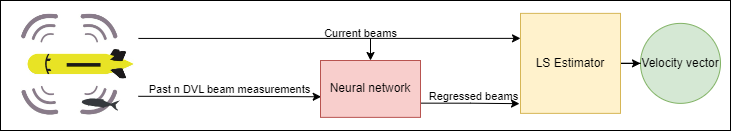
Figure 1: MissBeamNet framework utilizing past DVL beam measurements to regress the missing beams.

We consider two types of neural networks as our baseline network architectures. The first is based on a one-dimension convolution neural network (CNN), while the other is based on long-short-term memory (LSTM) cells. Both networks have been proven to work with time-series data, such as those considered in our scenario.

III-A Baseline Network Architectures

III-A1 Convolutional Neural Network

In CNN layers, there is a sparse interaction between the input and output, as appose to fully connected layers, where all the input parameters directly interact with the output. The convolution operator is a linear operator that involves multiplying an input with a kernel containing learned parameters. The kernel slides through the input, and the result is the sum of all the multiplications:

$$y_{t}=\sum_{k=1}^{p}x_{t+k}w_{k}$$ (10)

where $t$ is the timestamp, $p$ is the kernel length, $w$ is the learned kernel parameter, and $x$,$y$ are the input and output, respectively. The fact that CNN shares parameters by passing the same kernels through all the input makes CNN architectures very popular in situations with large inputs. Figure 2 describes our baseline CNN architecture, including network parameters, for a scenario of two missing beams. The network is a multi-head network where past DVL measurements are the input to the first head, and current DVL measurements are the input to the second head. The same structure and parameters are used when one or three beams are missing. The selected activation function between the layers is Relu and the stride and padding are set to one.

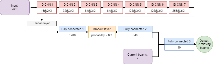
Figure 2: Baseline CNN architecture with an example of two missing beams.

III-A2 Long Short-Term Memory Network

LSTM is an advanced version of a recurrent neural network (RNN) and solves its shortcomings. RNNs are capable of handling temporal data by using information from prior inputs. However, if the sequence is long, the RNN may face a problem known as vanishing/exploding gradients [29]. For example, when a gradient is small, it may continue to decrease until the model is no longer learning. The LSTM addresses these problems using three types of gates: The forget gate, the input gate, and the output gate.
The role of the forget gate is to forget unwanted information from the previous output and current input:

$$f_{t}=\sigma(x_{t}U^{f}+h_{t-1}W^{f}+b_{f})$$ (11)

where $x_{t}$ is the input, $h_{t-1}$ is the output of the previous LSTM cell, $W^{f}$ and $b_{f}$ are the weights and biases of the forget gate, respectively. In (11) sigmoid function is employed to bring the parameter it wants to forget closer to zero. The output of the forget gate is then multiplied by the previous cell state. The role of the input gate is to update the cell state $C_{t-1}$, by first calculating the input gate $i_{t}$:

$$i_{t}=\sigma(x_{t}U^{i}+h_{t-1}W^{i}+b_{i})$$ (12)

where $U^{i}$ and $w^{i}$ are the gate weights and $b_{i}$ is the bias. Second, calculating the estimated cell state $\tilde{C_{t}}$:

$$\tilde{C_{t}}=tanh(x_{t}U^{g}+h_{t-1}W^{g}+b_{g})$$ (13)

where $U^{g}$ and $w^{g}$ are the gate weights and $b_{g}$ is the bias. The results of (11),(12), and (13) are used for the current cell state calculations:

$$C_{t}=f_{t}\cdot C_{t-1}+i_{t}\cdot\tilde{C_{t}}$$ (14)

As the name implies, the output gate $o_{t}$ determines which parameters are important as the output and next hidden state.

$$o_{t}=\sigma(x_{t}U^{o}+h_{t-1}W^{o}+b_{o})$$ (15)

where $U^{t}$ and $w^{t}$ are the gate weights and $b_{t}$ is the bias. The output gate results are then multiplied by a tanh layer of the cell state to calculate the current output and hidden state

$$h_{t}=o_{t}\cdot tanh(C_{t})$$ (16)

Figure 3 describes our LSTM baseline network structure. Previous beam measurements are used as input to the LSTM layers. After the LSTM features extraction, the features are concatenated with available beam measurements into a fully connected layer, which performs the final process resulting in the output of the regressed missing beams. Note that, like our baseline CNN network, this is a multi-head network where past DVL measurements are inputs to the first head, and current DVL measurements are inputs to the second head.

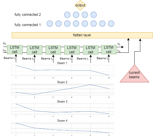
Figure 3: Baseline LSTM structure.

Figure 4 describes the LSTM architecture parameters in the scenario of two missing beams. The activation function between the layers is Relu. The same structure and parameters are also used when one or three beams are missing.

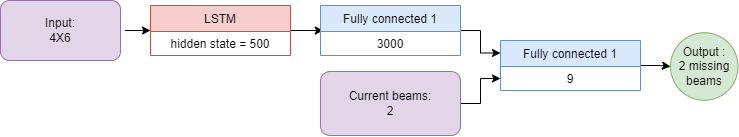
Figure 4: Baseline LSTM architecture with an example of two missing beams.

III-B Training Process

The training process of deep neural networks requires defining a loss function. The common loss functions for regression problems are mean absolute error (MAE) or mean squared error (MSE). In this paper, we use MSE loss defined by:

$$MSE=\frac{1}{n}\sum_{i=1}^{n}(y_{actual}-y_{predicted})^{2}$$ (17)

where $n$ is the number of samples, $y_{actual}$ is the target, and $y_{predicted}$ is the model output. Generally, the MSE loss function will try to adjust the model to better handle outliers than MAE due to the MSE squared error. However, in our scenarios, an AUV operates in varying sea conditions, therefore we adopt the MSE loss. During training, the loss function is calculated after each forward propagation in order to use the method of gradient descent and set the DNN initial weight and biases on values that will provide the desired result. Forward propagation is the process of the data going through all the layers of the architecture, like (10) for CNN and (11)-(16) for LSTM networks. After completing the forward propagation process, the back propagation process updates the weights and biases of all the layers with a gradient descent principle

$$\theta=\theta-\eta\nabla_{\theta}J(\theta)$$ (18)

where $\theta$ is the vector of weights and biases, $J(\theta)$ is the loss function with the DNN weights and biases set to $\theta$, $\nabla_{\theta}$ is the gradient operator, and $\eta$ is the learning rate.
The learning rate is a crucial hyperparameter, which dictates how fast the weights and biases change after each training batch. If the selected learning rate is too low, it might converge in a local minimum, and if it is too high, the model might not converge at a minimum. Our selected optimizer for all tested architectures is an adaptive moment estimation (ADAM) [30].

IV Analysis Results

IV-A Dataset Description

To examine the proposed approach, data from sea experiments were employed. All experiments were conducted in the Mediterranean Sea by the ”Snapir” (ECA A18D), a 5.5[m] long AUV capable of reaching 3000[m] depth. It is equipped with the Teledyne RDI Work Horse navigator DVL[31], which has a four-beams Janus convex configuration with a sample rate of $1$[Hz].

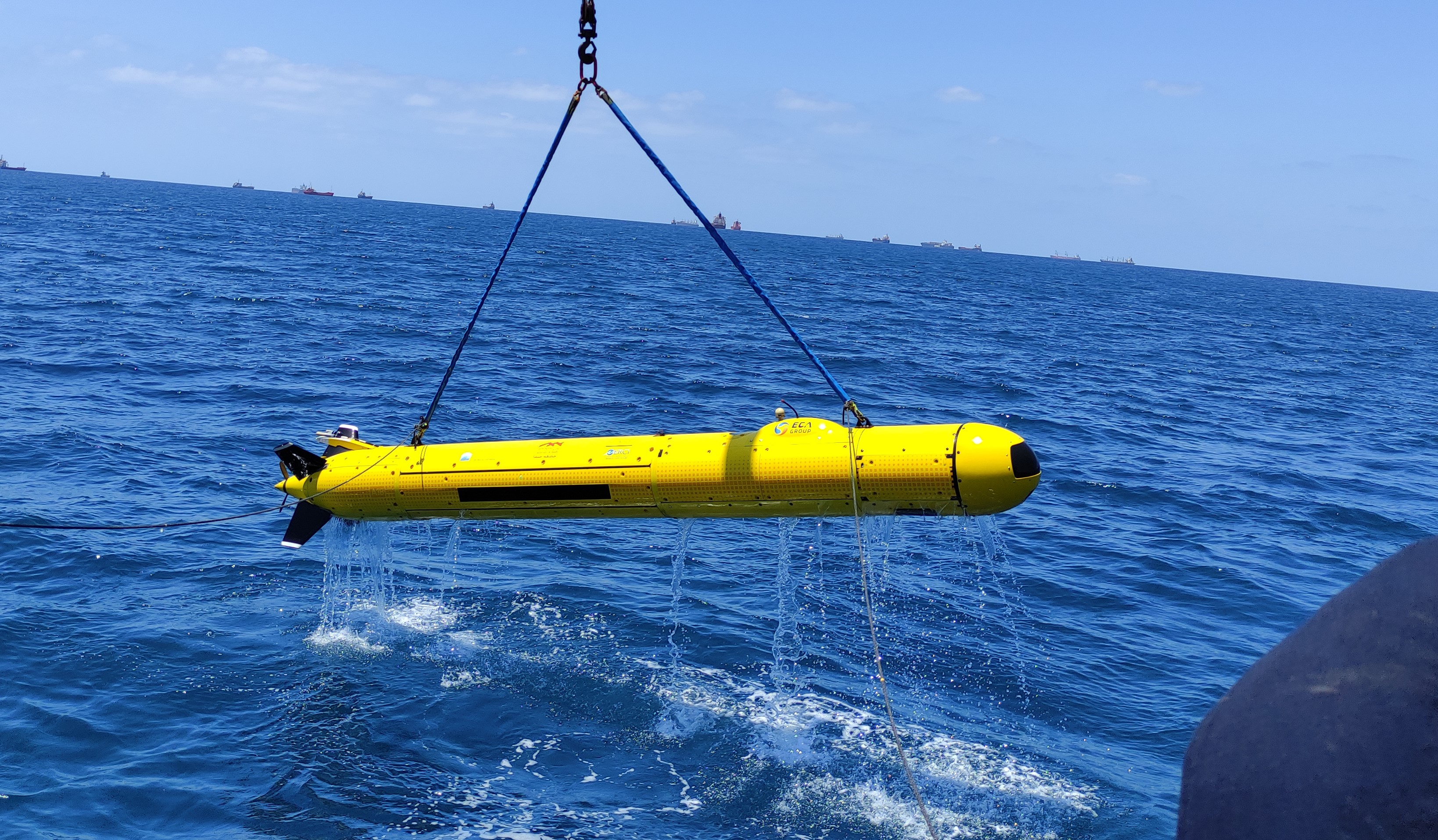
Figure 5: The ”Snapir” being pulled out of the water after a successful mission.

To train the deep neural network, first, all invalid DVL data was removed (some of the invalid readings occurred when actual beams were missing). Then, the data was divided into routes that the AUV performed. Approximately 60% of the missions were used as the training dataset and the rest as the test dataset. The training dataset comprised 23,243 samples corresponding to 387 minutes of recording, and the test dataset had 276 minutes of recording (16,618 samples).
Figure 6 shows an experiment with challenging dynamics which is part of the test dataset.

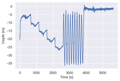
Figure 6: Experiment example from the test dataset.

The total of 663 minutes of recordings consists of two parts: 300 minutes from our initial data collection campaign [22] and 363 minutes in the current campaign. The complete dataset is publicly available at our GitHub https://github.com/ansfl/MissBeamNet.

IV-B Performance Metric

Performance metrics compare different models/methods and choose the one with the best performance. Throughout the research, we used the performance metric of root mean squared error (RMSE), which is widely used to evaluate models on regression tasks. RMSE is calculated by taking the root of the average of squared differences between the predicted values and the target values

$$RMSE=\sqrt{\frac{\sum_{i=1}^{n}(y_{actual}-y_{predicted})^{2}}{n}}$$ (19)

The RMSE results are in the same units as the original data, making it easy to interpret.

IV-C Baseline Architectures Comparison

To compare our two baseline architectures described in Section  III-B, we consider a scenario with two missing beams, namely, beams #1 and #2, and assume six past beam measurements are used. In addition to these two baseline architectures, we examine the possibility of using only past beam measurements instead of the baseline multi-head approach. These two architectures are denoted as CNN A and LSTM A. The results of the test dataset in terms of RMSE are presented in Figure 7.

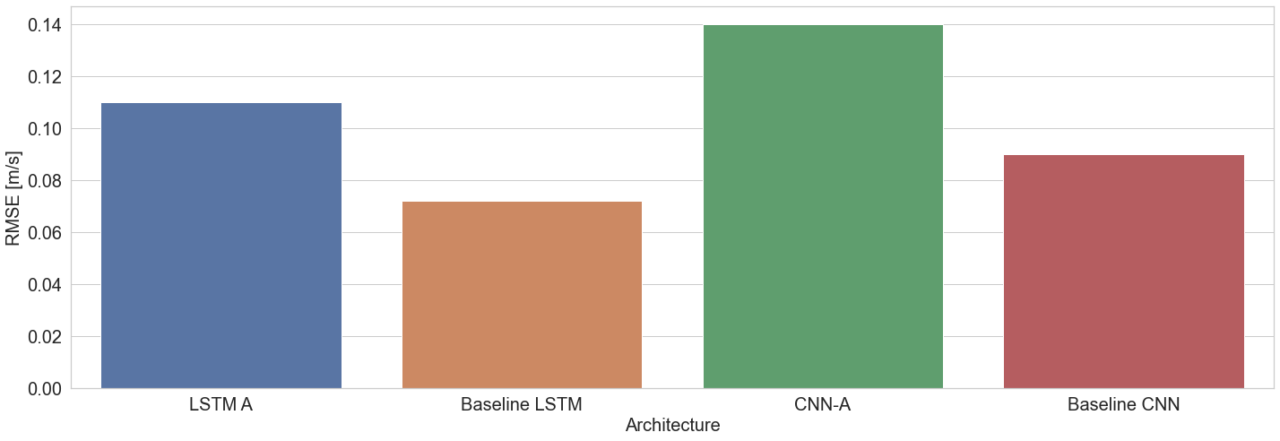
Figure 7: RMSE results for network architecture comparison.

The results shows that using the baseline architectures (multi-head) obtained better performance than working with all the inputs in a single head. In addition, the performance of the baseline LSTM showed an improvement of 27 % over the baseline CNN.

IV-D Number of Past Beam Measurement Influence

The number of past measurements utilized by the network is defined as the window-size length. The length of the optimal window size is crucial for model performance. The window size regularizes the model performance between the long and short movement patterns. If the selected window size is too short, the model might miss the pattern of the AUV movement, and if it is too long, the model might not react well enough to a movement that just started. Figure 8 shows the RMSE of the baseline LSTM model with different window-size lengths (between 3-10) when beams #1 and #2 are being regressed.

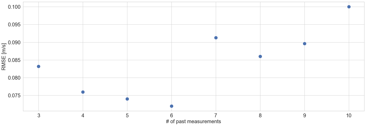
Figure 8: RMSE as a function of the window size for the baseline LSTM network.

The results suggest that the optimal window-size length on our dataset is six measurements.

IV-E Additional Input Information

To improve the model performance even further, additional inputs are considered.

1. Depth Sensor: The last depth sensor reading.

2. AUV Velocity Vector: Domain knowledge is used to transform the raw data (in this case, the beams) into meaningful features using feature engineering. Feature engineering is prevalent in classical machine learning methods, but less in deep neural networks. The assumption when using a neural network is thet model will learn the essential relations between features independently. The beams and the velocity vector are related, as the latter is estimated using the former. That is, the model is not receiving new information. Yet, in the proposed LSTM-based model, there are only two fully connected layers, and therefore feature engineering may help achieve better accuracy or shorten the network convergence time.

Figure 9 describes the performance of each input with our baseline LSTM architecture, including additional inputs of 1) depth, 2) velocity vector, and 3) depth and velocity vector. The tested case is when beams #1 and #2 are missing, and beams #3 and #4 are inserted as a two-phase input to our baseline LSTM network.

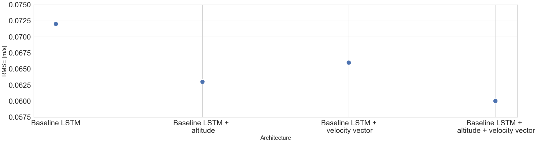
Figure 9: Velocity RMSE as a function of different input selection for our baseline LSTM network.

All of the additional inputs improved the performance of the baseline LSTM, and the best approach was obtained using all three input types - beam measurements (baseline), depth sensors, and the velocity vector. In this instance, there was a 16% improvement compared to the LSTM baseline.

IV-F Missing Beams Analysis

There are 14 combinations of missing beams: four combinations of one missing beam, six of two missing beams, and four of three missing beams. In the proposed approach a different network needs to be trained for each of those combinations. Training for all networks used the same hyper-parameters: MSE loss function with a learning rate of 0.00005, batch size of 1 sequence, and 150 epochs. In the following sections, we present the performance of our MissBeamNet approach compared to the average (baseline) and virtual beam approaches. For this analysis, we employed our baseline LSTM network described in Section 3.1.2. Based on the results of Section 4.4, we use six past DVL beam measurements and, based on Section 4.5, both the depth sensor reading and velocity vector were are added as additional inputs. The results were obtained on the testing dataset.

IV-F1 One missing beam

When one beam is missing, the least squared approach (4) can be used to obtain the estimated AUV velocity vector. Table I presents the results of estimating the missing beam, the speed error obtained when using the estimated fourth beam together with the measured three, and the improvement of our MissBeamNet approach over the two model-based approaches.

TABLE I: One missing beam scenario results on the test dataset

Case	Approach	Beam 1	Beam 2	Beam 3	Beam 4	Avg.
						results
Missing beam [m/s]	Average (baseline)	0.110	0.101	0.101	0.111	0.106
	Virtual beam	0.139	0.109	0.110	0.129	0.121
	MissBeamNet (ours)	0.065	0.048	0.034	0.067	0.053
Speed error [m/s]	Average (baseline)	0.066	0.061	0.061	0.067	0.064
	Virtual beam	0.079	0.065	0.066	0.077	0.072
	Three beams	0.450	0.437	0.438	0.449	0.443
	MissBeamNet (ours)	0.039	0.029	0.021	0.040	0.032
MissBeamNet improvement %	Average (baseline)	40.9	52.4	65.6	40.3	49.8
	Virtual beam	50.6	55.3	68.1	48.0	55.5
	Three beams	91.3	93.3	95.2	91.1	92.7

Both model-based and MissBeamNet methods were superior tp the three beams solution, indicating that regressing the fourth beam is critical to improving the AUV speed estimation accuracy. Specifically, MissBeamNet, improved the speed accuracy by over 90%. In addition, MissBeamNet performed significantly better than the model-based approaches, with a 40%-68% improvement. Taking the mean of performance of all four scenarios MissBeamNet improved the model-based approaches by over 49.8 %.

IV-F2 Two Missing Beams

When considering two missing beams, six different combinations exist. In such scenarios, the AUV velocity cannot be estimated. Following the same procedure as the previous one missing beam scenarios, Table II presents the results of two missing beams.

TABLE II: Two missing beam scenario results on the test dataset

Case	Approach	Beam 1,2	Beam 1,3	Beam 1,4	Beam 2,3	Beam 2,4	Beam 3,4	Avg. result
Missing beams [m/s]	Average (baseline)	0.106	0.106	0.111	0.101	0.107	0.106	0.106
	Virtual beam	0.121	0.121	0.131	0.110	0.119	0.120	0.120
	MissBeamNet (ours)	0.062	0.052	0.085	0.076	0.057	0.066	0.066
Speed error [m/s]	Average (baseline)	0.092	0.077	0.096	0.088	0.079	0.092	0.087
	Virtual beam	0.106	0.069	0.114	0.096	0.065	0.105	0.092
	MissBeamNet (ours)	0.055	0.057	0.075	0.066	0.061	0.058	0.062
MissBeamNet improvement %	Average (baseline)	40.2	25.9	21.9	25.0	22.8	36.9	28.7
	Virtual beam	48.1	17.4	34.2	31.25	6.15	44.7	30.3

The results show a significant difference between the speed error in each combination, even in the model-based approaches, emphasizing the problem’s complexity. Yet, in all cases, MissBeamNet was more accurate than the model-based approaches, with a minimum improvement of 20% that reached almost 50%. The average improvement over the baseline model-based approach was 28.7% compared to 49.8% when only one beam was missing. This is attributed to the model receiving less information from two current beams compared to three when only one is missing.

IV-F3 Three Missing Beams

Table III presents the results for the four scenarios in which three beams are missing.

TABLE III: Three missing beam scenario results on the test dataset

Case	Approach	Beam 1,2,3	Beam 2,3,4	Beam 1,2,4	Beam 1,3,4	Avg. results
Missing beams [m/s]	Average (baseline)	0.104	0.108	0.107	0.105	0.106
	Virtual beam	0.118	0.124	0.124	0.116	0.120
	MissBeamNet (ours)	0.071	0.073	0.077	0.071	0.073
Speed error [m/s]	Average (baseline)	0.102	0.108	0.106	0.103	0.105
	Virtual beam	0.102	0.109	0.111	0.099	0.105
	MissBeamNet (ours)	0.077	0.081	0.083	0.078	0.079
MissBeamNet improvement %	Average (baseline)	24.5	25.0	21.7	24.3	23.9
	Virtual beam	24.5	25.7	25.2	21.2	24.1

As expected, the speed error when three beams are missing is higher than in the two or one missing beams scenarios. Yet, MissBeamNet use improved results by at least 21% over the model-based approaches. For three missing beams, the average improvement was 24% compared to 28.7% when two beams were missing, only 4.7% less, indicating that even with only one beam at hand, the AUV velocity can be estimated.

IV-F4 Hyperparameter Tuning

One of the main challenges in deep learning research is to find the best combination of hyperparameters for the proposed architecture. Each architecture has several parameters that can influence model performance, including the number of layers, the number of parameters in each layer, the type of cost function, the learning rate, and batch size. To demonstrate the potential of hyperparameter tuning, we evaluated three different hyperparameters. The first was the learning rate, which affects how much each batch changes the weights and biases III-B. The second hyper parameter was the number of hidden parameters in the LSTM layer $h_{t}$ III-A2, and the third hyperparameter is the number of parameters in the LSTM output. To test the importance of hyperparameter tuning, each parameter was set with a few available options, and a seed was set (equal initialization in each run). We focused on a one missing beam scenario, which has four options - missing beam $\#1,\#2,\#3$, or $\#4$. For each case, 15 randomly selected combinations of the three hyperparameters were examined.

TABLE IV: hyperparameters tuning

Case	Approach	Beam 1	Beam 2	Beam 3	Beam 4
Missing beam [m/s]	Before tuning	0.065	0.048	0.034	0.067
	After tuning	0.011	0.017	0.02	0.012
Speed error [m/s]	Before tuning	0.039	0.029	0.021	0.040
	After tuning	0.007	0.010	0.012	0.007
Learning rate	Before tuning	5e-05	5e-05	5e-05	5e-05
	After tuning	1e-04	1e-04	5e-05	1e-05
hidden LSTM parameters $h_{t}$	Before tuning	500	500	500	500
	After tuning	250	750	750	100
LSTM output parameters	Before tuning	7	7	7	7
	After tuning	7	5	7	5
MissBeamNet Tuning improvement %	Average (baseline)	89.4	83.6	80.3	89.5
	Virtual beam	91.1	84.6	81.8	90.9
	Three beams	98.4	97.7	97.2	98.4
	Before tuning	82.2	67.5	42.8	82.5

Table IV presents the potential of hyperparameter tuning. It is important to note that out of the 15 tested hyperparameter combinations, only a few were better than the results before tuning. Yet, they were able to improve the missing beam estimation and, consequently, reduce the speed error and increase the rate of improvement compared to the two model-based approaches.

V Conclusions

Here, we presented MissBeamNet, a deep learning-based framework developed to compensate for partial DVL measurement scenarios (1, 2, or 3 missing beams). To that end, an LSTM-based dedicated DNN was derived. We demonstrated that the best input to the network is past DVL measurements, past depth sensor measurements, previous velocity vectors, and the currently available measured beams. Once the missing beams are regressed, they are combined with the available beams and plugged into the classical model-based approach to estimate the AUV velocity vector.
To evaluate MissBeamNet, sea experiments with the University of Haifa’s ”Snapir” AUV were conducted. The data included several trajectories collected for different purposes and under various sea conditions. We provide a thorough analysis of all 14 missing beam combinations and explore several means to enhance our baseline architecture. The results show that MissBeamNet allows estimating the missing DVL beams and, consequently, the AUV velocity vector. Additionally, MissBeamNet significantly improves the accuracy of the velocity vector in all examined scenarios compared to the model-based approaches. The improvement of all three missing beam combinations was above 20 % over the model-based approaches. For two missing beams, performance was generally better compared to three missing beams since the model uses one additional measured beam. Finally, we show that hyperparameters-tuned models improve the accuracy of MissBeamNet by more than $40\%$.

References

- [1] Q. Luo, Y. Shao, J. Li, X. Yan and C. Liu, A multi-AUV cooperative navigation method based on the augmented adaptive embedded cubature Kalman filter algorithm., Neural Comput and Applic vol. 34, pp. 18975–18992 2022.
- [2] M. Mohammadi, M.M. Arefi, N. Vafamand and O. Kaynak Control of an AUV with completely unknown dynamics and multi-asymmetric input constraints via off-policy reinforcement learning, Neural Comput and Applic vol. 34, pp. 5255–5265 2022.
- [3] RR.B. Wynn, V.A.I. Huvenne, T.P. Le Bas, B.J. Murton, D.P. Connelly, B.J. Bett, H.A. Ruhl, K.J. Morris, J. Peakall, D.R. Parsons, E.J. Sumner, S.E. Darby, R.M. Dorrell and J.E. Hunt, Autonomous Underwater Vehicles (AUVs): their past, present and future contributions to the advancement of marine geoscience Marine Geology., vol. 352, pp. 451-468. 2014.
- [4] E. Bovio, D. Cecchi and F. Baralli, Autonomous underwater vehicles for scientific and naval operations, Annual Reviews in Control,Vol. 30, Issue 2, 2006.
- [5] A. Kume, T. Maki, T. Sakamaki, and T. Ura, A Method for Obtaining High-Coverage 3D Images of Rough Seafloor Using AUV – Real-Time Quality Evaluation and Path-Planning, Journal of robotics and mechatronics,vol.25 (2), pp.364-374, 2013.
- [6] Niu, H., Adams, S., Lee, K., Husain, T. and N. Bose, Applications of Autonomous Underwater Vehicles in Offshore petroleum industry environmental effects monitoring, Journal of Canadian Petroleum Technology, vol.48, 2009.
- [7] Z. Hongwei, Z. Shitong, W. Yanhui, L. Yuhong, Y.Yanan, Z. Tian and B. Hongyu,Subsea pipeline leak inspection by autonomous underwater vehicle, Applied ocean research, Vol.107, pp.102321, 2021.
- [8] F. Maussang, J. Chanussot and A. Hetet, Automated segmentation of SAS images using the mean - standard deviation plane for the detection of underwater mines, Oceans 2003. Celebrating the Past … Teaming Toward the Future, IEEE, vol.4, pp. 2155–2160, 2003.
- [9] A.Palomer, P. Ridao and D. Ribas, Multibeam 3D underwater SLAM with probabilistic registration, Sensors vol. 16, 4, pp. 560, 2016.
- [10] Y. K. Thong, M. S. Woolfson, J. A. Crowe, B. R. Hayes-Gill, and R. E. Challis, Dependence of inertial measurements of distance on accelerometer noise Meas. Sci. Technol., vol. 13 (8), pp. 1163, 2002.
- [11] A. Karmozdi, M. Hashemi, H. Salarieh and A. Alasty, INS-DVL Navigation Improvement Using Rotational Motion Dynamic Model of AUV, IEEE Sensors Journal, vol. 20, no. 23, pp. 14329-14336, 2020.
- [12] M.Emami and M.R. Taben, A novel intelligent adaptive Kalman Filter for estimating the Submarine’s velocity: With experimental evaluation , Ocean Engineering, vol. 158, pp. 403-411, 2018.
- [13] B. Allotta, A. Caiti, R. Costanzi, F. Fanelli, D. Fenucci, E. Meli, and A. Ridolfi, A new AUV navigation system exploiting unscented Kalman filter, Ocean Engineering, vol. 113, pp. 121-132, 2016.
- [14] P. Liu, B. Wang, G. Li, D. Hou, Z. Zhu and Z. Wang, SINS/DVL Integrated Navigation Method With Current Compensation Using RBF Neural Network, IEEE Sensors Journal, vol. 22, no. 14, pp. 14366-14377, 2022.
- [15] P. Liu, B. Wang, Z. Deng, M. Fu INS/DVL/PS tightly coupled underwater navigation method with limited DVL measurements., IEEE Sensors, vol. 18, no. 7, pp. 2994-3002, 2018.
- [16] Z. Yonggang, Y. Ding, L. Ning. A tightly integrated SINS/DVL navigation method for autonomous underwater vehicle, International Conference on Computational and Information Sciences, pp. 1107-1110, 2013.
- [17] A. Tal, I. Klein, and R. Katz. Inertial navigation system/Doppler velocity log fusion with partial DVL measurements, IEEE Sensors, vol. 17, no. 2, pp. 415, 2017.
- [18] I. Klein, Data-Driven Meets Navigation: Concepts, Models, and Experimental Validation, 2022 DGON Inertial Sensors and Systems (ISS), pp. 1-21, 2022.
- [19] N.Cohen and I. klein, BeamsNet: A data-driven approach enhancing Doppler velocity log measurements for autonomous underwater vehicle navigation, Engineering Applications of Artificial Intelligence, vol. 114, pp. 1055216, 2022.
- [20] X. Zhang, B. He, G. Li, X. Mu, Y. Zhou and T. Mang, NavNet: AUV navigation through deep sequential learning, IEEE Access, vol. 8, pp. 59845-59861, 2020.
- [21] M. Yona and I. Klein, Compensating for Partial Doppler Velocity Log Outages by Using Deep- Learning Approaches, IEEE International Symposium on Robotic and Sensors Environments (ROSE), pp. 1-5, 2021.
- [22] A. Shurin, A. Saraev ,M. Yona, Y. Gutnik, S. Faber, A. Etzion and I. Klein, The autonomous platforms inertial dataset, IEEE Access, vol. 10, pp. 10191-10201, 2022.
- [23] The Hatter department of marine technologies, ocean instruments: https://www.marinetech.haifa.ac.il/ocean-instruments
- [24] Teledyne RD Instruments, Adcp Coordinate Transformation Formulas and Calculation.
- [25] P. A. Miller, J. A. Farrell, Y. Zhao and V. Djapic, Autonomous Underwater Vehicle Navigation, IEEE Journal of Oceanic Engineering, vol. 35, no. 3, pp. 663-678, 2010.
- [26] C.T. Crowe, D.F. Elger, and J.A. Roberson, Engineering Fluid Mechanics, Boston: Cengage Learning, pp.21-27, 2016.
- [27] I. Klein and Y. Lipman, Continuous INS/DVL Fusion in Situations of DVL Outages 2020 IEEE/OES Autonomous Underwater Vehicles Symposium (AUV), pp. 1-6,2020.
- [28] I. Klein, Y. Gutnik and Y. Lipman, Estimating DVL Velocity in Complete Beam Measurement Outage Scenarios, IEEE Sensors Journal, vol. 22, no. 21, pp. 20730-20737, 2022,
- [29] R. Pascanu, T. Mikolov and Y. Bengio, On the difficulty of training recurrent neural networks Proceedings of the 30th International Conference on Machine Learning, pp.1310-1318, 2013.
- [30] P. Diederik and B. Jimmy Adam: A Method for Stochastic Optimization, 3rd International Conference for Learning Representations, 2015.
- [31] Teledyne marine manual for the Teledyne RDI Work Horse navigator DVL.