A Simple Algorithm For Scaling Up Kernel Methods

Abstract

The recent discovery of the equivalence between infinitely wide neural networks (NNs) in the lazy training regime and Neural Tangent Kernels (NTKs) Jacot et al. (2018) has revived interest in kernel methods. However, conventional wisdom suggests kernel methods are unsuitable for large samples due to their computational complexity and memory requirements. We introduce a novel random feature regression algorithm that allows us (when necessary) to scale to virtually infinite numbers of random features. We illustrate the performance of our method on the CIFAR-10 dataset.

1 Introduction

Modern neural networks operate in the over-parametrized regime, which sometimes requires orders of magnitude more parameters than training data points. Effectively, they are interpolators (see, Belkin (2021)) and overfit the data in the training sample, with no consequences for the out-of-sample performance. This seemingly counterintuitive phenomenon is sometimes called “benign overfit” (Bartlett et al., 2020; Tsigler and Bartlett, 2020).

In the so-called lazy training regime Chizat et al. (2019), wide neural networks (many nodes in each layer) are effectively kernel regressions, and “early stopping” commonly used in neural network training is closely related to ridge regularization (Ali et al., 2019). See, Jacot et al. (2018); Hastie et al. (2019); Du et al. (2018, 2019a); Allen-Zhu et al. (2019). Recent research also emphasizes the “double descent,” in which expected forecast error drops in the high-complexity regime. See, for example, Zhang et al. (2016); Belkin et al. (2019a, b); Spigler et al. (2019); Belkin et al. (2020).

These discoveries made many researchers argue that we need to gain a deeper understanding of kernel methods (and, hence, random feature regressions) and their link to deep learning. See, e.g., Belkin et al. (2018). Several recent papers have developed numerical algorithms for scaling kernel-type methods to large datasets and large numbers of random features. See, e.g., Zandieh et al. (2021); Ma and Belkin (2017); Arora et al. (2019a); Shankar et al. (2020). In particular, Arora et al. (2019b) show how NTK combined with the support vector machines (SVM) (see also Fernández-Delgado et al. (2014)) perform well on small data tasks relative to many competitors, including the highly over-parametrized ResNet-34. In particular, while modern deep neural networks do generalize on small datasets (see, e.g., Olson et al. (2018)), Arora et al. (2019b) show that kernel-based methods achieve superior performance in such small data environments. Similarly, Du et al. (2019b) find that the graph neural tangent kernel (GNTK) dominates graph neural networks on datasets with up to 5000 samples. Shankar et al. (2020) show that, while NTK is a powerful kernel, it is possible to build other classes of kernels (they call Neural Kernels) that are even more powerful and are often at par with extremely complex deep neural networks.

In this paper, we develop a novel form of kernel ridge regression that can be applied to any kernel and any way of generating random features. We use a doubly stochastic method similar to that in Dai et al. (2014), with an important caveat: We generate (potentially large, defined by the RAM constraints) batches of random features and then use linear algebraic properties of covariance matrices to recursively update the eigenvalue decomposition of the feature covariance matrix, allowing us to perform the optimization in one shot across a large grid of ridge parameters.

The paper is organized as follows. Section 2 discusses related work. In Section 3, we provide a novel random feature regression mathematical formulation and algorithm. Then, Section 4 and Section 5 present numerical results and conclusions, respectively.

2 Related Work

Before the formal introduction of the NTK in Jacot et al. (2018), numerous papers discussed the intriguing connections between infinitely wide neural networks and kernel methods. See, e.g., Neal (1996); Williams (1997); Le Roux and Bengio (2007); Hazan and Jaakkola (2015); Lee et al. (2018); Matthews et al. (2018); Novak et al. (2018); Garriga-Alonso et al. (2018); Cho and Saul (2009); Daniely et al. (2016); Daniely (2017). As in the standard random feature approximation of the kernel ridge regression (see Rahimi and Recht (2007)), only the network’s last layer is trained in the standard kernel ridge regression. A surprising discovery of Jacot et al. (2018) is that (infinitely) wide neural networks in the lazy training regime converge to a kernel even though all network layers are trained. The corresponding kernel, the NTK, has a complex structure dependent on the neural network’s architecture. See also Lee et al. (2019), Arora et al. (2019a) for more results about the link between NTK and the underlying neural network, and Novak et al. (2019) for an efficient algorithm for implementing the NTK. In a recent paper, Shankar et al. (2020) introduce a new class of kernels and show that they perform remarkably well on even very large datasets, achieving a 90% accuracy on the CIFAR-10 dataset. While this performance is striking, it comes at a huge computational cost. Shankar et al. (2020) write:

“CIFAR-10/CIFAR-100 consist of $60,000$ $32\times 32\times 3$ images and MNIST consists of $70,000$ $28\times 28$ images. Even with this constraint, the largest compositional kernel matrices we study took approximately 1000 GPU hours to compute. Thus, we believe an imperative direction of future work is reducing the complexity of each kernel evaluation. Random feature methods or other compression schemes could play a significant role here.

In this paper, we offer one such highly scalable scheme based on random features. However, computing the random features underlying the Neural Kernels of Shankar et al. (2020) would require developing non-trivial numerical algorithms based on the recursive iteration of non-linear functions. We leave this as an important direction for future research.

As in standard kernel ridge regressions, we train our random feature regression on the full sample. This is a key computational limitation for large datasets. After all, one of the reasons for the success of modern deep learning is the possibility of training them using stochastic gradient descent on mini-batches of data. Ma and Belkin (2017) shows how mini-batch training can be applied to kernel ridge regression. A key technical difficulty arises because kernel matrices (equivalently, covariance matrices of random features) have eigenvalues that decay very quickly. Yet, these low eigenvalues contain essential information and cannot be neglected. Our regression method can be easily modified to allow for mini-batches. Furthermore, it is known that mini-batch linear regression can even lead to performance gains in the high-complexity regime. As LeJeune et al. (2020) show, one can run regression on mini-batches and then treat the obtained predictions as an ensemble. LeJeune et al. (2020) prove that, under technical conditions, the average of these predictions attains a lower generalization error than the full-train-sample-based regression. We test this mini-batch ensemble approach using our method and show that, indeed, with moderately-sized mini-batches, the method’s performance matches that of the full sample regression.

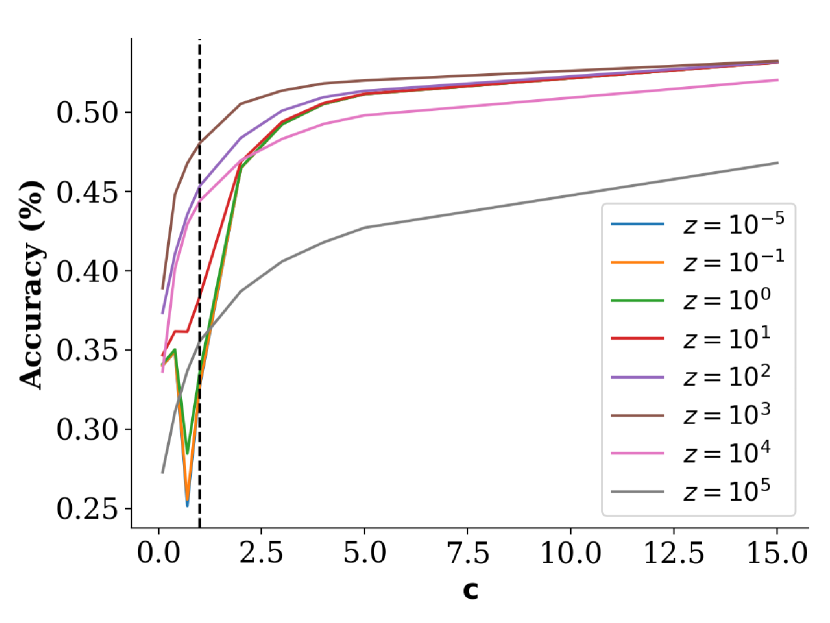
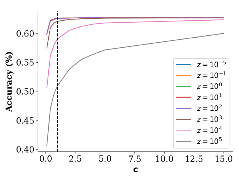
Moreover, there is an intriguing connection between mini-batch regressions and spectral dimensionality reduction. By construction, the feature covariance matrix with a mini-batch of size $B$ has at most $B$ non-zero eigenvalues. Thus, a mini-batch effectively performs a dimensionality reduction on the covariance matrix. Intuitively, we expect that the two methods (using a mini-batch of size $B$ or using the full sample but only keeping $B$ largest eigenvalues) should achieve comparable performance. We show that this is indeed the case for small sample sizes. However, the spectral method for larger-sized samples ($N\geq 10000$) is superior to the mini-batch method unless we use very large mini-batches. For example, on the full CIFAR-10 dataset, the spectral method outperforms the mini-batch approach by 3% (see Section 4 for details).

3 Random Features Ridge Regression and Classification

Suppose that we have a train sample $(X,y)\ =\ (x_{i},y_{i})_{i=1}^{N},\ x_{i}\in{\mathbb{R}}^{d},\ y_{i}\in{\mathbb{R}},$ so that $X\in{\mathbb{R}}^{N\times d},\ y\in{\mathbb{R}}^{N\times 1}.$ Following Rahimi and Recht (2007) we construct a large number of random features $f(x;\theta_{p}),\ p=1,\ldots,P,$ where $f$ is a non-linear function and $\theta_{p}$ are sampled from some distribution, and $P$ is a large number. We denote $S=f(X;\theta)\in{\mathbb{R}}^{N\times P}$ as the train sample realizations of random features. Following Rahimi and Recht (2007), we consider the random features ridge regression,

$$\beta(z)\ =\ (S^{\top}S/N+zI)^{-1}S^{\top}y/N\,,$$ (1)

as an approximation for kernel ridge regression when $P\to\infty$. For classification problems, it is common to use categorical cross-entropy as the objective. However, as Belkin (2021) explains, minimizing the mean-squared error with one-hot encoding often achieves superior generalization performance. Here, we follow this approach. Given the $K$ labels, $k=1,\ldots,K,$ we build the one-hot encoding matrix $Q=(q_{i,k})$ where $q_{i,k}={\bf 1}_{y_{i}=k}.$ Then, we get

$$\beta(z)\ =\ (S^{\top}S/N+zI)^{-1}S^{\top}Q/N\ \in\ {\mathbb{R}}^{P\times K}\,.$$ (2)

Then, for each test feature vector ${\bf s}=f({\bf x};\theta)\in{\mathbb{R}}^{P},$ we get a vector $\beta(z)^{\top}{\bf s}\in{\mathbb{R}}^{K}$. Next, define the actual classifier as

$$k({\bf x};z)\ =\ \arg\max\{\beta(z)^{\top}{\bf s}\}\ \in\ \{1,\cdots,K\}\,.$$ (3)

3.1 Dealing with High-Dimensional Features

A key computational (hardware) limitation of kernel methods comes from the fact that, when $P$ is large, computing the matrix $S^{\top}S\in{\mathbb{R}}^{P\times P}$ becomes prohibitively expensive, in particular, because $S$ cannot even be stored in RAM. We start with a simple observation that the following identity implies that storing all these features is not necessary:

$$(S^{\top}S/N+zI)^{-1}S^{\top}\ =\ S^{\top}(SS^{\top}/N+zI)^{-1}\,,$$ (4)

and therefore we can compute $\beta(z)$ as

$$\beta(z)\ =\ S^{\top}(SS^{\top}/N+zI)^{-1}y/N\,.$$ (5)

Suppose now we split $S$ into multiple blocks, $S_{1},\ldots,S_{K},$ where $S_{k}\in{\mathbb{R}}^{N\times P_{1}}$ for all $k=1,\ldots,K$, for some small $P_{1},$ with $KP_{1}=P.$ Then,

$$\Psi=SS^{\top}\ =\ \sum_{k=1}^{K}S_{k}S_{k}^{\top}$$ (6)

can be computed by generating the blocks $S_{k},$ one at a time, and recursively adding $S_{k}S_{k}^{\top}$ up. Once $\Psi$ has been computed, one can calculate its eigenvalue decomposition, $\Psi=VDV^{\top},$ and then evaluate $Q(z)=(\Psi/N+zI)^{-1}y/N\ =\ V(D+zI)^{-1}V^{\top}y/N\in{\mathbb{R}}^{N}$ in one go for a grid of $z.$ Then, using the same seeds, we can again generate the random features $S_{k}$ and compute $\beta_{k}(z)=S_{k}^{\top}Q(z)\in{\mathbb{R}}^{P_{1}}.$ Then, $\beta(z)=(\beta_{k}(z))_{k=1}^{K}\in{\mathbb{R}}^{P}\,.$ The logic described above is formalized in Algorithm 1.

Algorithm 1 FABReg

$P_{1}$, $P$, $X\in{\mathbb{R}}^{N\times d}$, $y\in{\mathbb{R}}^{N}$, $z$, $voc\_curve$

$blocks\leftarrow P//P_{1}$

$k\leftarrow 0$

$\Psi\leftarrow 0_{N\times N}$

while $k<blocks$ do

     Generate $S_{k}\in{\mathbb{R}}^{N\times P_{1}}$ Use $k$ as seed

     $\Psi\leftarrow\Psi+S_{k}S_{k}\top$

     if $k$ in $voc\_curve$ then

         $DV\leftarrow eigen(\frac{\Psi}{N})$

         $Q_{k}(z)\leftarrow V(D+zI)^{-1}V^{\top}\frac{y}{N}$ $\triangleright$ Store $Q_{k}(z)$

     end if

     $k=k+1$

end while

$DV\leftarrow eigen(\frac{\Psi}{N})$

$Q(z)\leftarrow V(D+zI)^{-1}V^{\top}\frac{y}{N}$

$k\leftarrow 0$

while $k<blocks$ do

     (re-)Generate $S_{k}\in{\mathbb{R}}^{N\times P_{1}}$ $\triangleright$ Use $k$ as seed

     $\beta_{k}(z)\leftarrow S^{\top}_{k}Q(z)$

     $\hat{y}\mathrel{+}=S_{k}\beta_{k}$

end while

3.2 Dealing with Massive Datasets

The above algorithm relies crucially on the assumption that $N$ is small. Suppose now that the sample size $N$ is so large that storing and eigen-decomposing the matrix $SS^{\top}\in{\mathbb{R}}^{N\times N}$ becomes prohibitively expensive. In this case, we proceed as follows.

Define for all $k=1,\ldots,K$

$$\Psi_{k}\ =\ \sum_{\kappa=1}^{k}S_{k}S_{k}^{\top}\in{\mathbb{R}}^{N\times N},\ \Psi_{0}=0_{N\times N}\,,$$ (7)

and let $\lambda_{1}(A)\geq\cdots\geq\lambda_{N}(A)$ be the eigenvalues of a symmetric matrix $A\in{\mathbb{R}}^{N\times N}.$ Our goal is to design an approximation to $(\Psi_{K}+zI)^{-1},$ based on a simple observation that the eigenvalues of the empirically observed $\Psi_{k}$ matrices tend to decay very quickly, with only a few hundreds of largest eigenvalues being significantly different from zero. In this case, we can fix a $\nu\in\mathbb{N}$ and design a simple, rank$-\nu$ approximation to $\Psi_{K}$ by annihilating all eigenvalues below $\lambda_{\nu}(\Psi_{K}).$ As we now show, it is possible to design a recursive algorithm for constructing such an approximation to $\Psi_{K},$ dealing with small subsets of random features simultaneously. To this end, we proceed as follows.

Suppose we have constructed an approximation $\hat{\Psi}_{k}\in{\mathbb{R}}^{N\times N}$ to $\Psi_{k}$ with rank $\nu,$ and let $V_{k}\in{\mathbb{R}}^{N\times\nu}$ be the corresponding matrix of orthogonal eigenvectors for the non-zero eigenvalues, and $D_{k}\in{\mathbb{R}}^{\nu\times\nu}$ the diagonal matrix of eigenvalues so that $\hat{\Psi}_{k}=V_{k}D_{k}V_{k}^{\top}$ and $V_{k}^{\top}V_{k}=I_{\nu\times\nu}$. Instead of storing the full $\hat{\Psi}_{k}$ matrix, we only need to store the pair $(V_{k},D_{k}).$ For all $k=1,\ldots,K$, we now define

$$\tilde{\Psi}_{k+1}\ =\ \hat{\Psi}_{k}\ +\ S_{k+1}S_{k+1}^{\top}\,.$$ (8)

This $N\times N$ matrix is a theoretical construct. We never actually compute it (see Algorithm 2). Let $\Theta_{k}=I-V_{k}V_{k}^{\top}$ be the orthogonal projection on the kernel of $\hat{\Psi}_{k},$ and

$$\tilde{S}_{k+1}\ =\ \Theta_{k}S_{k+1}\ =\ S_{k+1}-\underbrace{V_{k}}_{N\times\nu}(\underbrace{V_{k}^{\top}S_{k+1}}_{\nu\times P_{1}})$$ (9)

be $S_{k+1}$ orthogonalized with respect to the columns of $V_{k}.$ Then, we define $\tilde{W}_{k+1}=\tilde{S}_{k+1}(\tilde{S}_{k+1}\tilde{S}_{k+1}^{\top})^{-1/2}$ to be the orthogonalized columns of $\tilde{S}_{k+1},$ and $\hat{V}_{k+1}=[V_{k},\tilde{W}_{k+1}]$. To compute $\tilde{S}_{k+1}(\tilde{S}_{k+1}\tilde{S}_{k+1}^{\top})^{-1/2},$ we use the following lemma that, once again, uses smart eigenvalue decomposition techniques to avoid dealing with the $N\times N$ matrix $\tilde{S}_{k+1}\tilde{S}_{k+1}^{\top}$.

Lemma 1.

Let $\underbrace{\tilde{S}_{k+1}^{\top}\tilde{S}_{k+1}}_{\nu\times\nu}=W\delta\tilde{W}^{\top}$ be the eigenvalue decomposition of $\tilde{S}_{k+1}^{\top}\tilde{S}_{k+1}.$ Then, $\tilde{W}=\tilde{S}_{k+1}W\delta^{-1/2}$ is the matrix of eigenvectors of $\tilde{S}_{k+1}\tilde{S}_{k+1}^{\top}$ for the non-zero eigenvalues. Thus,

$$\tilde{S}_{k+1}(\tilde{S}_{k+1}\tilde{S}_{k+1}^{\top})^{-1/2}\ =\ \tilde{W}_{k+1}\,.$$ (10)

By construction, the columns of $\hat{V}_{k+1}$ form an orthogonal basis of the span of the columns of $V_{k},S_{k+1},$ and hence

$$\Psi_{k+1,*}\ =\ \hat{V}_{k+1}^{\top}\tilde{\Psi}_{k+1}\hat{V}_{k+1}\ \in\ {\mathbb{R}}^{(P_{1}+\nu)\times(P_{1}+\nu)}$$ (11)

has the same non-zero eigenvalues as $\tilde{\Psi}_{k+1}.$ We then define $\tilde{V}_{k+1}\in{\mathbb{R}}^{(P_{1}+\nu)\times\nu}$ to be the matrix with eigenvectors of $\Psi_{k+1,*}$ for the largest $\nu$ eigenvalues, and we denote the diagonal matrix of these eigenvalues by $D_{k+1}\in{\mathbb{R}}^{\nu\times\nu}$, and then we define $V_{k+1}\ =\ \hat{V}_{k+1}\tilde{V}_{k+1}\,.$ Then, $\hat{\Psi}_{k+1}\ =\ V_{k+1}D_{k+1}V_{k+1}\ =\ \Pi_{k+1}\tilde{\Psi}_{k+1}\Pi_{k+1}\,,$ where $\Pi_{k+1}\ =\ \hat{V}_{k+1}\tilde{V}_{k+1}\tilde{V}_{k+1}^{\top}\hat{V}_{k+1}^{\top}$ is the orthogonal projection onto the eigen-subspace of $\tilde{\Psi}_{k+1}$ for the largest $\nu$ eigenvalues.

Lemma 2.

We have $\hat{\Psi}_{k}\leq\tilde{\Psi}_{k}\leq\Psi_{K}$ and

$$\|\Psi_{k}-\hat{\Psi}_{k}\|\ \leq\ \sum_{i=1}^{k}\lambda_{\nu+1}(\Psi_{i})\ \leq\ k\,\lambda_{\nu+1}(\Psi_{K})\,,$$ (12)

and

$$\|(\Psi_{k+1}+zI)^{-1}-(\hat{\Psi}_{k+1}+zI)^{-1}\|\ \leq\ z^{-2}\sum_{i=1}^{k}\lambda_{\nu+1}(\Psi_{i})\,.$$ (13)

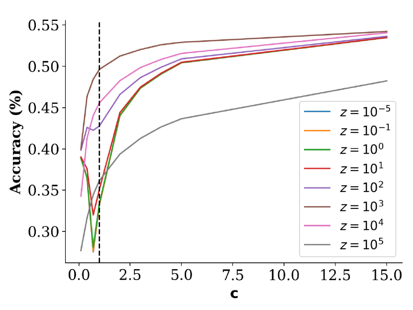
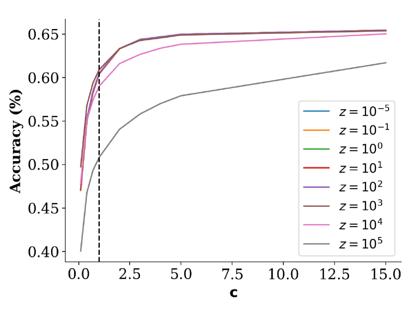
There is another important aspect of our algorithm: It allows us to directly compute the performance of models with an expanding level of complexity. Indeed, since we load random features in batches of size $P_{1},$ we generate predictions for $P\in[P_{1},2P_{1},\cdots,KP_{1}].$ This is useful because we might use it to calibrate the optimal degree of complexity and because we can directly study the double descent-like phenomena, see, e.g., Belkin et al. (2019a) and Nakkiran et al. (2021). That is the effect of complexity on the generalization error. In the next section, we do this. As we show, consistent with recent theoretical results Kelly et al. (2022), with sufficient shrinkage, the double descent curve disappears, and the performance becomes almost monotonic in complexity. Following Kelly et al. (2022), we name this phenomenon the virtue of complexity (VoC) and the corresponding performance plots the VoC curves. See, Figure 6 below.

We call this algorithm Fast Annihilating Batch Regression (FABReg) as it annihilates all eigenvalues below $\lambda_{\nu}(\Psi_{K})$ and allows to solve the random features ridge regression in one go for a grid of $z$. Algorithm 2 formalizes the logic described above.

Algorithm 2 FABReg-$\nu$

$\nu$, $P_{1}$, $P$, $X\in{\mathbb{R}}^{N\times d}$, $y\in{\mathbb{R}}^{N}$, $z$, $voc\_curve$

$blocks\leftarrow P//P_{1}$

$k\leftarrow 0$

while $k<blocks$ do

     Generate $S_{k}\in{\mathbb{R}}^{N\times P_{1}}$ $\triangleright$ Use $k$ as seed to generate the random features

     if $k=0$ then

         $\tilde{d},\tilde{V}\leftarrow eigen(S^{\top}_{k}S_{k})$

         $V\leftarrow S_{k}\tilde{V}diag(\tilde{d})^{-\frac{1}{2}}$

         $V_{0}\leftarrow V_{:,min(\nu,P_{1})}$ $\triangleright$ Save $V_{0}$

         $d_{0}\leftarrow\tilde{d}_{:min(\nu,P_{1})}$ $\triangleright$ Save $d_{0}$

         if k in $voc\_curve$ then

              $Q_{0}(z)\leftarrow V_{0}(diag(d_{0})+zI)^{-1}V_{0}^{\top}y$ $\triangleright$ Save $Q_{0}(z)$

         end if

     else if $k>0$ then

         $\tilde{S_{k}}\leftarrow(I-V_{k-1}V^{\top}_{k-1})S_{k}$

         $\Gamma_{k}\leftarrow\tilde{S^{\top}_{k}}\tilde{S_{k}}$

         $\delta_{k},W_{k}\leftarrow eigen(\Gamma_{k})$

         Keep top min($\nu,P1$) eigenvalues and eigenvectors from $\delta_{k},W_{k}$

         $\tilde{W_{k}}\leftarrow\tilde{S_{k}}W_{k}diag(\delta_{k})^{-\frac{1}{2}}$

         $\hat{V_{k}}\leftarrow[V_{k-1},\tilde{W_{k}}]$

         $\bar{V_{k}}\leftarrow\hat{V^{\top}_{k}}V_{k-1}$

         $\bar{W_{k}}\leftarrow\bar{V_{k}}diag(d_{k-1})\bar{V^{\top}_{k}}$

         $\bar{S_{k}}\leftarrow\hat{V^{\top}_{k}}S_{k}$

         $\bar{Z_{k}}\leftarrow\bar{S_{k}}S^{\top}_{k}$

         $\Psi_{*}\leftarrow\bar{W_{k}}\bar{Z_{k}}$

         $d_{k},V_{k}\leftarrow eigen(\Psi_{*})$

         Keep top min($\nu,P1$) eigenvalues and eigenvectors from $d_{k},V_{k}$

         $V_{k}\leftarrow\hat{V_{k}}V_{k}$ $\triangleright$ Save $d_{k},V_{k}$

         if k in $voc\_curve$ then

              $Q_{k}(z)\leftarrow V_{k}(diag(d_{k})+zI)^{-1}V_{k}^{\top}y$ $\triangleright$ Save $Q_{k}(z)$

         end if

     end if

     $k=k+1$

end while

$k\leftarrow 0$

while $k<blocks$ do

     (re-)Generate $S_{k}\in{\mathbb{R}}^{N\times P_{1}}$ $\triangleright$ Use $k$ as seed to generate the random features

     $\beta_{k}(z)\leftarrow S^{\top}_{k}Q_{k}(z)$

     $\hat{y}\mathrel{+}=S_{k}\beta_{k}$

end while

4 Numerical Results

This section presents several experimental results on different datasets to evaluate FABReg’s performance and applications. In contrast to the most recent computational power demand in kernel methods, e.g., Shankar et al. (2020), we ran all experiments on a laptop, a MacBook Pro model A2485, equipped with an M1 Max with a 10-core CPU and 32 GB RAM.

4.1 A comparison with sklearn

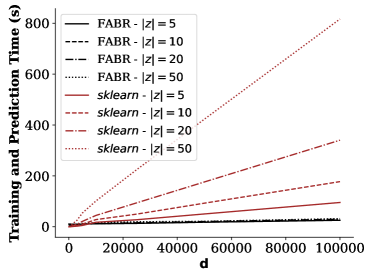
We now aim to show FABReg’s training and prediction time with respect to the number of features $d$. To this end, we do not use any random feature projection or the rank-$\nu$ matrix approximation described in Section 3.1. We draw $N=5000$ i.i.d. samples from $\otimes_{j=1}^{d}\mathcal{N}(0,1)$ and let

$$y_{i}=x_{i}\beta+\epsilon_{i}\quad\forall i=1,\ldots,N,$$

where $\beta\sim\otimes_{j=1}^{d}\mathcal{N}(0,1)$, and $\epsilon_{i}\sim\mathcal{N}(0,1)$ for all $i=1,\ldots,N$. Then, we define

$$y_{i}=\begin{cases}1&\text{if $y_{i}>\text{median}(\boldsymbol{y})$},\\ 0&\text{otherwise}\end{cases}\quad\forall i=1,\ldots,N.$$

Next, we create a set of datasets for classification with varying complexity $d$ and keep the first 4000 samples as the training set and the remaining 1000 as the test set. We show in Figure 1 the average training and prediction time (in seconds) of FABReg with a different number of regularizers ( we denote this number by $|z|$) and sklearn RidgeClassifier with an increasing number of features $d$. The training and prediction time is averaged over five independent runs. As one can see, our method is drastically faster when $d>10000$. E.g., for $d=100000$ we outperform sklearn by approximately 5 and 25 times for $|z|=5$ and $|z|=50$, respectively. Moreover, one can notice that the number of different shrinkages $|z|$ does not affect FABReg. We report a more detailed table with average training and prediction time and standard deviation in Appendix B.

Figure 1: The figure above compares FABReg training and prediction time, shown on the y-axis, in black, against sklearn’s RidgeClassifier, in red, for an increasing amount of features, shown on the x-axis, and the number of shrinkages $z$. Here, $|z|$ denotes the number of different values of $z$ for which we perform the training.

4.2 Experiments on Real Datasets

We assess FABReg’s performance on both small and big datasets regimes for further evaluation. For all experiments, we perform a random features kernel ridge regression for demeaned one-hot labels and solve the optimization problem using FABReg as described in Section 3.

4.2.1 Data Representation

Table 1: The table below shows the average test accuracy and standard deviation of ResNet-34, CNTK, and FABR on the subsampled CIFAR-10 datasets. The test accuracy is average over twenty independent runs.

n	ResNet-34	14-layer CNTK	z=1	z=100	z=10000	z=100000
10	14.59% $\pm$ 1.99%	15.33% $\pm$ 2.43%	18.50% $\pm$ 2.18%	18.50% $\pm$ 2.18%	18.42% $\pm$ 2.13%	18.13% $\pm$ 2.01%
20	17.50% $\pm$ 2.47%	18.79% $\pm$ 2.13%	20.84% $\pm$ 2.38%	20.85% $\pm$ 2.38%	20.78% $\pm$ 2.35%	20.13% $\pm$ 2.34%
40	19.52% $\pm$ 1.39%	21.34% $\pm$ 1.91%	25.09% $\pm$ 1.76%	25.10% $\pm$ 1.76%	25.14% $\pm$ 1.75%	24.41% $\pm$ 1.88%
80	23.32% $\pm$ 1.61%	25.48% $\pm$ 1.91%	29.61% $\pm$ 1.35%	29.60% $\pm$ 1.35%	29.62% $\pm$ 1.39%	28.63% $\pm$ 1.66%
160	28.30% $\pm$ 1.38%	30.48% $\pm$ 1.17%	34.86% $\pm$ 1.12%	34.87% $\pm$ 1.12%	35.02% $\pm$ 1.11%	33.54% $\pm$ 1.24%
320	33.15% $\pm$ 1.20%	36.57% $\pm$ 0.88%	40.46% $\pm$ 0.73%	40.47% $\pm$ 0.73%	40.66% $\pm$ 0.72%	39.34% $\pm$ 0.72%
640	41.66% $\pm$ 1.09%	42.63% $\pm$ 0.68%	45.68% $\pm$ 0.71%	45.68% $\pm$ 0.72%	46.17% $\pm$ 0.68%	44.91% $\pm$ 0.72%
1280	49.14% $\pm$ 1.31%	48.86% $\pm$ 0.68%	50.30% $\pm$ 0.57%	50.32% $\pm$ 0.56%	51.05% $\pm$ 0.54%	49.74% $\pm$ 0.42%

Figure 2: CNN architecture used to extract image features.

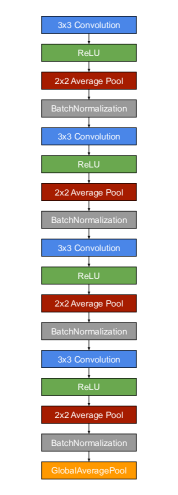
FABReg requires, like any standard kernel methods or randomized-feature techniques, a good data representation. Usually, we don’t know such a representation a-priori, and learning a good kernel is outside the scope of this paper. Therefore, we build a simple Convolutional Neural Network (CNN) mapping $h:{\mathbb{R}}^{d}\to{\mathbb{R}}^{D}$; that extracts image features $\tilde{x}\in{\mathbb{R}}^{D}$ for some sample $x\in{\mathbb{R}}^{d}$. The CNN is not optimized; we use it as a simple random feature mapping. The CNN architecture, shown in Fig. 2, alternates a $3\times 3$ convolution layer with a ReLU activation function, a $2\times 2$ Average Pool, and a BatchNormalization layer Ioffe and Szegedy (2015). Convolutional layers weights are initialized using He Uniform He et al. (2015). To vectorize images, we use a global average pooling layer that has proven to enforce correspondences between feature maps and to be more robust to spatial translations of the input Lin et al. (2013). We finally obtain the train and test random features realizations $s=f(\tilde{x},\theta)$. Specifically, we use the following random features mapping

$$s_{i}=\sigma(W\tilde{x}),$$ (14)

where $W\in{\mathbb{R}}^{P\times D}$ with $w_{i,j}\sim\mathcal{N}(0,1)$ and $\sigma$ is some elementwise activation function. This can be described as a one-layer neural network with random weights $W$. To show the importance of over-parametrized models, throughout the results, we report the complexity, $c$, of the model as $c=P/N$, that is, the ratio between the parameters (dimensions) and the number of observations. See Belkin et al. (2019a); Hastie et al. (2019); Kelly et al. (2022).

4.2.2 Small Datasets

We now study the performance of FABReg on the subsampled CIFAR-10 dataset Krizhevsky et al. (2009). To this end, we reproduce the same experiment described in Arora et al. (2019b). In particular, we obtain random subsampled training set $(y;X)=(y_{i};x_{i})_{i=1}^{n}$ where $n\in\{10,20,40,80,160,320,640,1280\}$ and test on the whole test set of size 10000. We make sure that exactly $n/10$ sample from each image class is in the training sample. We train FABReg using random features projection of the subsampled training set

$$S=\sigma(Wg(X))\in{\mathbb{R}}^{n\times P},$$

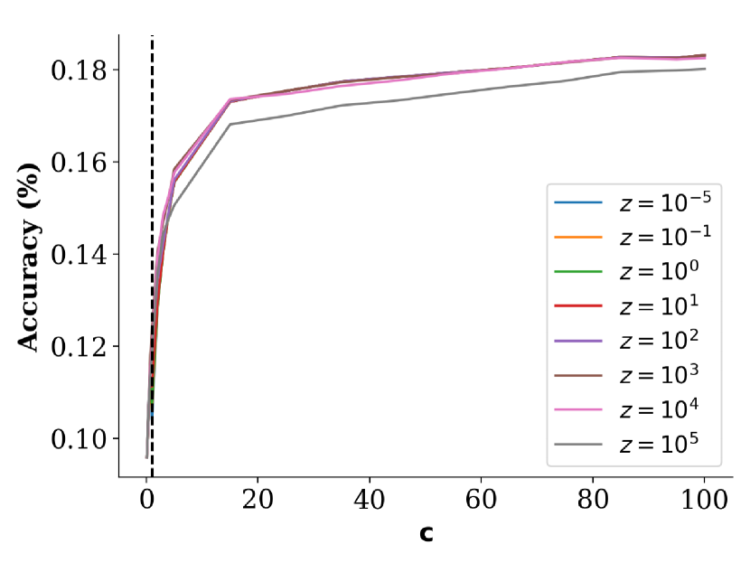
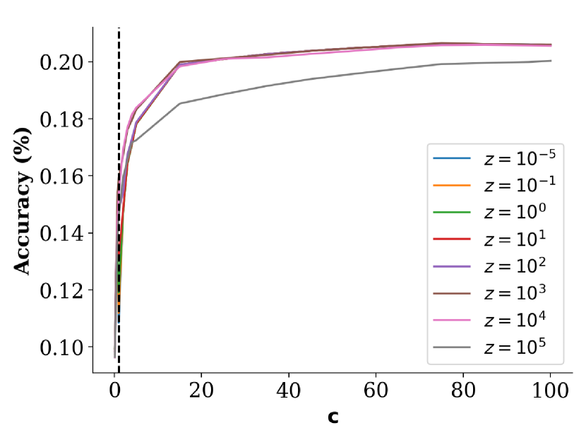
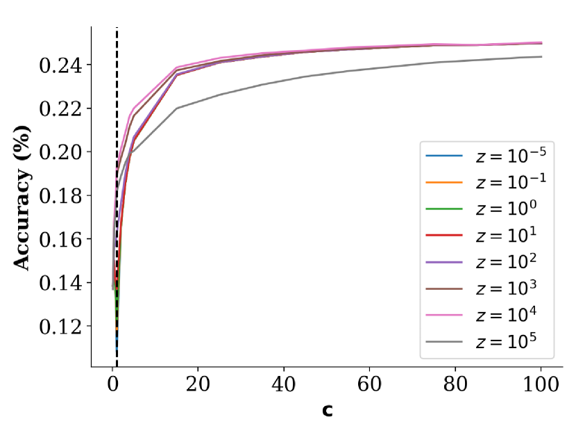
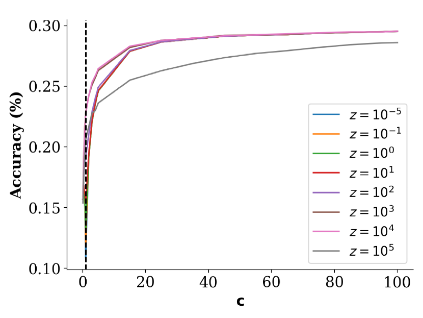
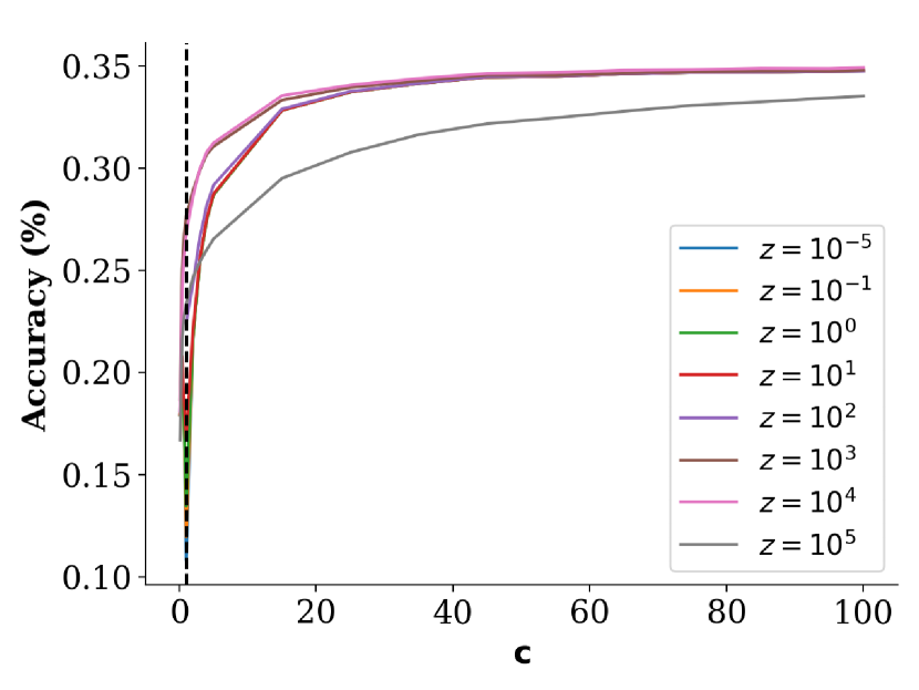
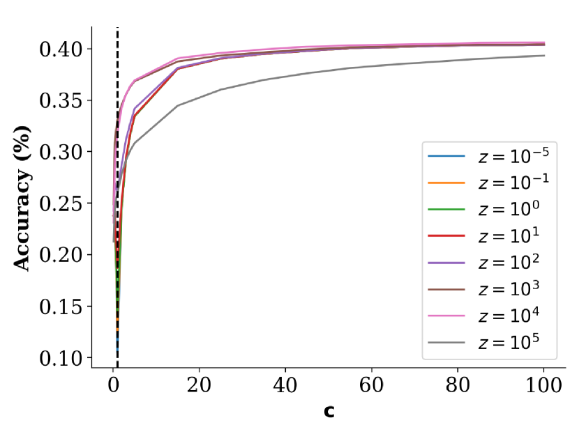
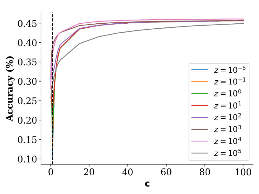
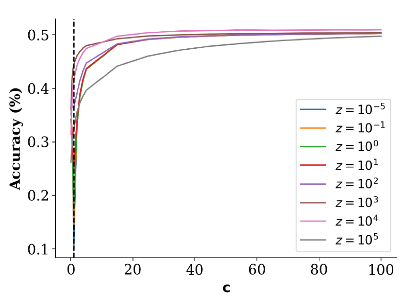
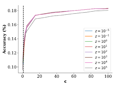
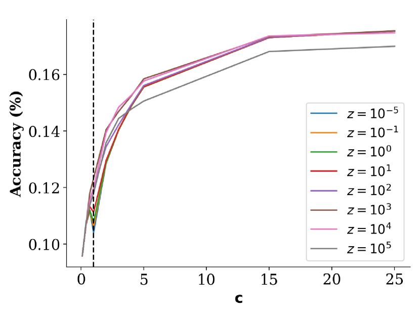
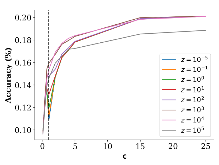
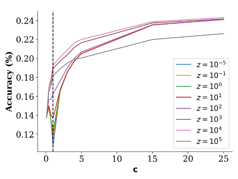
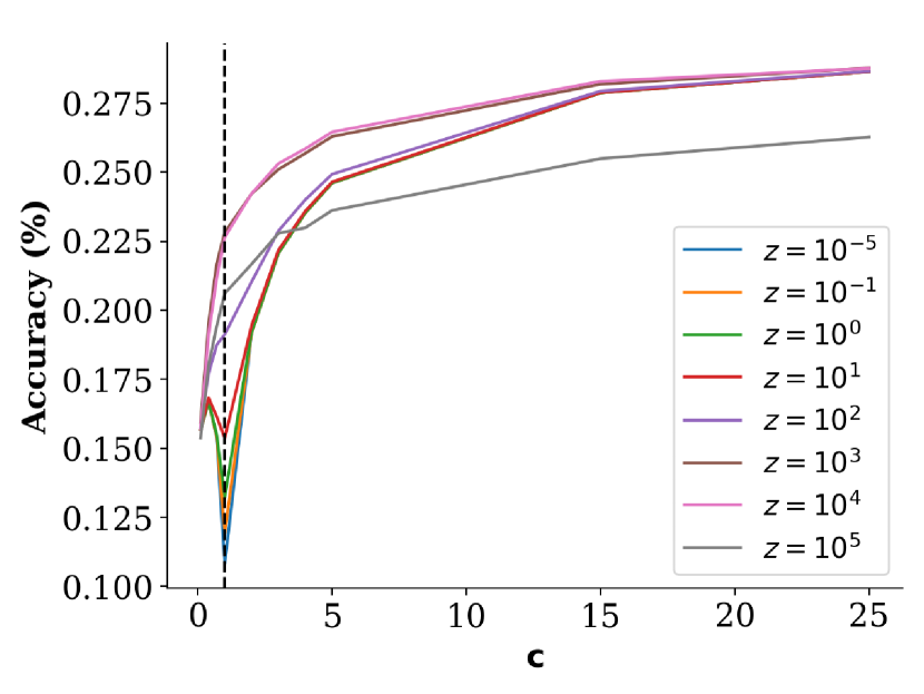
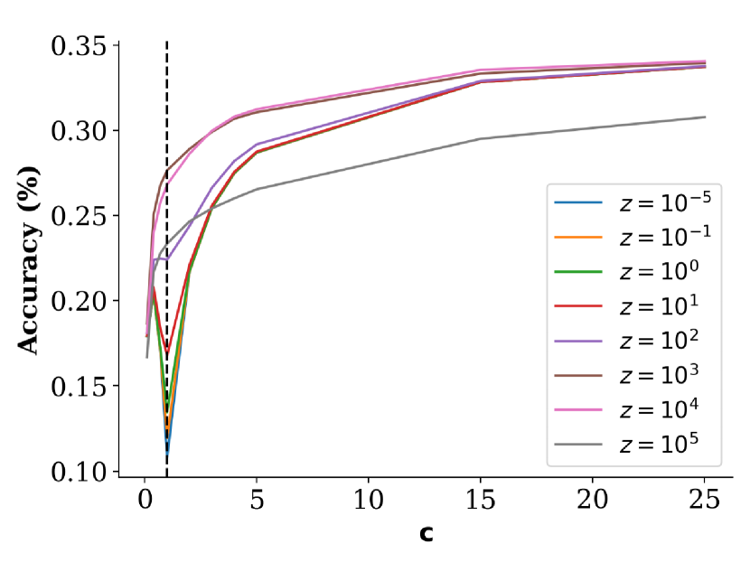
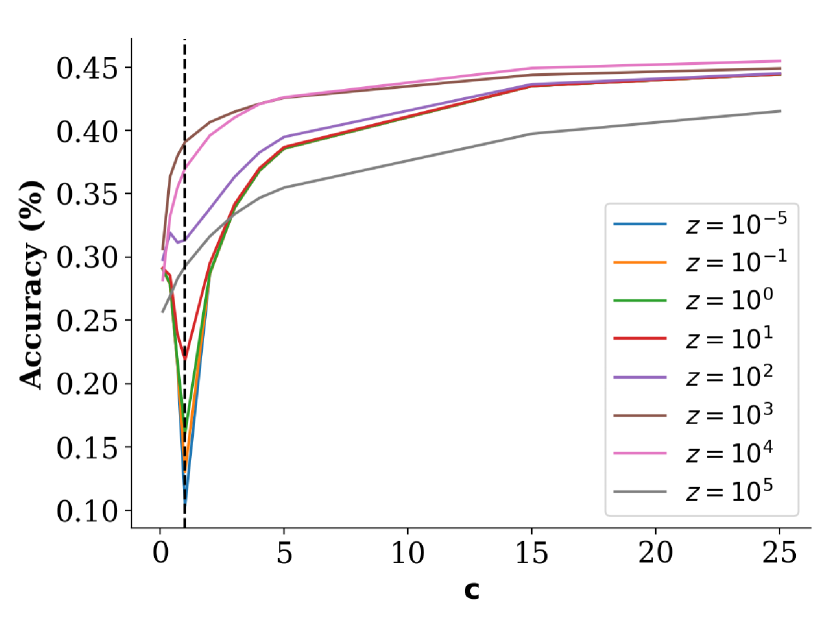
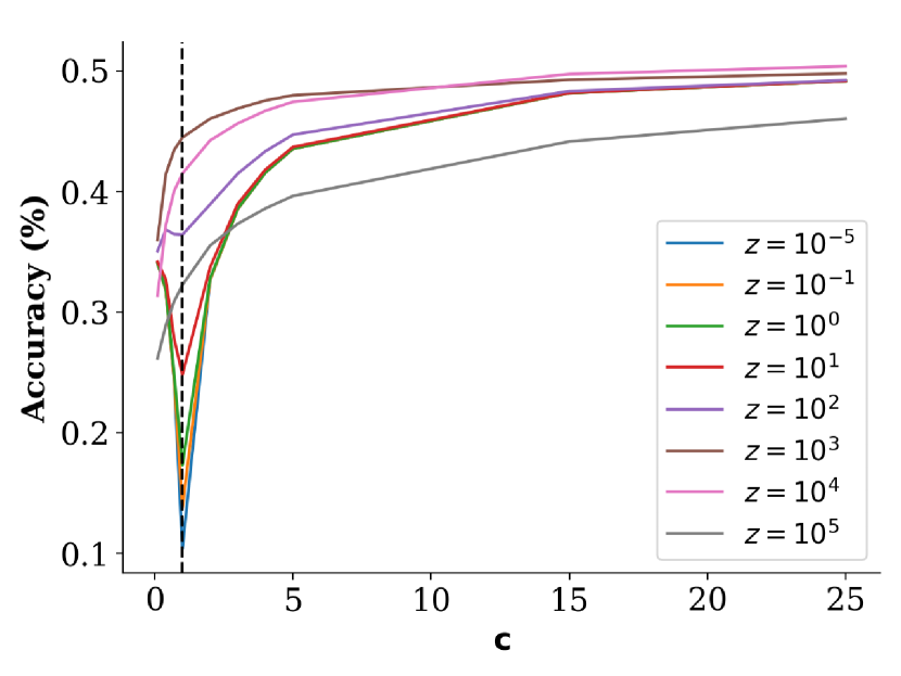
where $g$ is an untrained CNN from Figure 2, randomly initialized using He Uniform distribution. In this experiment, we push the model complexity $c$ to 100; in other words, FABReg’s number of parameters equals a hundred times the number of observations in the subsample. As $n$ is small, we deliberately do not perform any low-rank covariance matrix approximation. Finally, we run our model twenty times and report the mean out-of-sample performance and the standard deviation. We report in Table 1 FABReg’s performance for different shrinkages ($z$) together with ResNet-34 and the 14-layers CNTK. Without any complicated random feature projection, FABReg can outperform both ResNet-34 and CNTK. FABReg’s test accuracy increases with the model’s complexity $c$ on different ($n$) subsampled CIFAR-10 datasets. We show Figure 3 as an example for $n=10$. Additionally, we show, to better observe the double descent phenomena, truncated curves at $c=25$ for all CIFAR-10 subsamples in Figure 4. The full curves are shown in Appendix B. To sum up this section findings:

• FABReg, with enough complexity together and a simple random feature projection, is able to outperform deep neural networks (ResNet-34) and CNTKs.

• FABReg always reaches the maximum accuracy beyond the interpolation threshold.

• Moreover, if the random feature ridge regression shrinkage $z$ is sufficiently high, the double descent phenomenon disappears, and the accuracy does not drop at the interpolation threshold point, i.e., when $c=1$ or $n=P$. Following Kelly et al. (2022), we call this phenomenon virtue of complexity (VoC).

Figure 3: The figures above show FABReg’s test accuracy increases with the model’s complexity $c$ on the subsampled CIFAR-10 dataset for $n=10$. The test accuracy is averaged over five independent runs.

(a) $n=10$

(b) $n=20$

(c) $n=40$

(d) $n=80$

(e) $n=160$

(f) $n=320$

(g) $n=640$

(h) $n=1280$

Figure 4: The figures above show FABReg’s test accuracy increases with the model’s complexity $c$ on different ($n$) subsampled CIFAR-10 datasets. The expanded dataset follows similar patterns. We truncate the curve for $c>25$ to better show the double descent phenomena. The full curves are shown in Appendix B. Notice that when the shrinkage is sufficiently high, the double descent disappears, and the accuracy monotonically increases in complexity. Following Kelly et al. (2022), we name this phenomenon the virtue of complexity (VoC). The test accuracy is averaged over 20 independent runs.

(a) $n=2560$

(b) $n=50000$

Figure 5: The figures above show FABReg’s test accuracy increases with the model’s complexity $c$ on the subsampled CIFAR-10 dataset 5(a) and the full CIFAR-10 dataset 5(b). FABReg is trained using a $\nu=2000$ low-rank covariance matrix approximation. Notice that we still observe a (shifted) double descent when $\nu\approx n.$ The same phenomenon disappears when $\nu\ll n.$ The test accuracy is averaged over five independent runs.

4.2.3 Big Datasets

In this section, we repeat the same experiments described in Section 4.2.2, but we extend the training set size $n$ up to the full CIFAR-10 dataset. For each $n$, we train FABReg, FABReg-$\nu$ with a rank-$\nu$ approximation as described in Algorithm 2, and the min-batch FABReg. We use $\nu=2000$ and $\text{batch size}=2000$ in the last two algorithms. Following Arora et al. (2019b), we train ResNet-34 as the benchmark for 160 epochs, with an initial learning rate of 0.001 and a batch size of 32. We decrease the learning rate by ten at epochs 80 and 120. ResNet-34 always reaches close to perfect accuracy on the training set, i.e., above 99%. We run each training five times and report mean out-of-sample performance and its standard deviation. As the training sample is sufficiently large already, we set the model complexity to only $c=15$, meaning that for the full sample, FABReg performs a random feature ridge regression with $P=7.5\times 10^{5}$. We report the results in Tables 4.2.3 and 3.

Table 2: The table below shows the average test accuracy and standard deviation of ResNet-34 and FABR on the subsampled and full CIFAR-10 dataset. The test accuracy is average over five independent runs.

n	ResNet-34	z=1	z=100	z=10000	z=100000
2560	48.12% $\pm$ 0.69%	52.24% $\pm$ 0.29%	52.45% $\pm$ 0.21%	54.29% $\pm$ 0.44%	48.28% $\pm$ 0.37%
5120	56.03% $\pm$ 0.82%	55.34% $\pm$ 0.32%	55.74% $\pm$ 0.34%	58.29% $\pm$ 0.20%	52.06% $\pm$ 0.08%
10240	63.21% $\pm$ 0.26%	58.36% $\pm$ 0.45%	58.86% $\pm$ 0.54%	62.17% $\pm$ 0.35%	55.75% $\pm$ 0.18%
20480	69.24% $\pm$ 0.47%	61.08% $\pm$ 0.17%	61.65% $\pm$ 0.27%	65.12% $\pm$ 0.19%	59.34% $\pm$ 0.14%
50000	75.34% $\pm$ 0.21%	66.38% $\pm$ 0.00%	66.98% $\pm$ 0.00%	68.62% $\pm$ 0.00%	63.25% $\pm$ 0.00%

Table 3: The table below shows the average test accuracy and standard deviation of FABReg-$\nu$ and mini-batch FABReg on the subsampled and full CIFAR-10 dataset. The test accuracy is average over five independent runs.

	$z=1$		$z=100$		$z=10000$		$z=100000$
FABReg	batch $=2000$	$\nu=2000$	batch $=2000$	$\nu=2000$	batch $=2000$	$\nu=2000$	batch $=2000$	$\nu=2000$
n
2560	53.13% $\pm$ 0.38%	53.48% $\pm$ 0.22%	53.15% $\pm$ 0.42%	53.63% $\pm$ 0.24%	52.01% $\pm$ 0.51%	54.05% $\pm$ 0.44%	46.78% $\pm$ 0.52%	48.23% $\pm$ 0.34%
5120	57.68% $\pm$ 0.18%	57.63% $\pm$ 0.19%	57.70% $\pm$ 0.16%	57.63% $\pm$ 0.18%	56.83% $\pm$ 0.27%	57.53% $\pm$ 0.11%	51.42% $\pm$ 0.22%	51.75% $\pm$ 0.14%
10240	59.79% $\pm$ 0.35%	61.20% $\pm$ 0.39%	59.79% $\pm$ 0.35%	61.20% $\pm$ 0.38%	58.63% $\pm$ 0.28%	60.63% $\pm$ 0.21%	53.73% $\pm$ 0.37%	55.16% $\pm$ 0.34%
20480	61.56% $\pm$ 0.35%	63.50% $\pm$ 0.12%	61.55% $\pm$ 0.37%	63.50% $\pm$ 0.13%	60.90% $\pm$ 0.20%	62.92% $\pm$ 0.12%	57.10% $\pm$ 0.19%	58.40% $\pm$ 0.21%
50000	62.74% $\pm$ 0.10%	65.45% $\pm$ 0.18%	62.74% $\pm$ 0.10%	65.44% $\pm$ 0.18%	62.35% $\pm$ 0.05%	65.04% $\pm$ 0.19%	59.99% $\pm$ 0.02%	61.71% $\pm$ 0.09%

The experiment delivers a number of additional conclusions:

• First, we observe that, while for small train sample sizes of $n\leq 10000$, simple kernel methods achieve performance comparable with that of DNNs, this is not the case for $n>20000.$ Beating DNNs on big datasets with shallow methods requires more complex kernels, such as those in Shankar et al. (2020); Li et al. (2019).

• Second, we confirm the findings of Ma and Belkin (2017); Lee et al. (2020) suggesting that the role of small

  eigenvalues is important. For example, FABReg-$\nu$ with $\nu=2000$ loses several percent of accuracy on larger datasets.

• Third, surprisingly, both the mini-batch FABReg and FABReg-$\nu$ sometimes achieve higher accuracy than the full sample regression on moderately-sized datasets. See Tables 2 and 3. Understanding these phenomena is an interesting direction for future research.

• Fourth, the double descent phenomenon naturally appears for both FABReg-$\nu$ and the mini-batch FABReg but only when $\nu\approx n$ or $\text{batch size}\approx n$. However, the double descent phenomenon disappears when $\nu\ll n$. This intriguing finding is shown in Figure 5 for FABReg-$\nu$, and in Appendix B for the mini-batch FABReg.

• Fifth, on average, FABReg-$\nu$ outperforms mini-batch FABReg on larger datasets.

5 Conclusion and Discussion

The recent discovery of the equivalence between infinitely wide neural networks (NNs) in the lazy training regime and neural tangent kernels (NTKs) Jacot et al. (2018) has revived interest in kernel methods. However, these kernels are extremely complex and usually require running on big and expensive computing clusters Avron et al. (2017); Shankar et al. (2020) due to memory (RAM) requirements. This paper proposes a highly scalable random features ridge regression that can run on a simple laptop. We name it Fast Annihilating Batch Regression (FABReg). Thanks to the linear algebraic properties of covariance matrices, this tool can be applied to any kernel and any way of generating random features. Moreover, we provide several experimental results to assess its performance. We show how FABReg can outperform (in training and prediction speed) the current state-of-the-art ridge classifier’s implementation. Then, we show how a simple data representation strategy combined with a random features ridge regression can outperform complicated kernels (CNTKs) and over-parametrized Deep Neural Networks (ResNet-34) in the few-shot learning setting. The experiments section concludes by showing additional results on big datasets. In this paper, we focus on very simple classes of random features. Recent findings (see, e.g., Shankar et al. (2020)) suggest that highly complex kernel architectures are necessary to achieve competitive performance on large datasets. Since each kernel regression can be approximated with random features, our method is potentially applicable to these kernels as well. However, directly computing the random feature representation of such complex kernels is non-trivial and we leave it for future research.

Appendix A Proofs

Proof of Lemma 2.

We have

$$\Psi_{k+1}\ =\ \Psi_{k}\ +\ S_{k+1}S_{k+1}^{\prime}$$ (15)

$$\tilde{\Psi}_{k+1}\ =\ \hat{\Psi}_{k}\ +\ S_{k+1}S_{k+1}^{\prime}$$

$$\hat{\Psi}_{k+1}\ =\ P_{k+1}\tilde{\Psi}_{k+1}P_{k+1}\,.$$

By the definition of the spectral projection, we have

$$\|\tilde{\Psi}_{k+1}-\hat{\Psi}_{k+1}\|\ \leq\ \lambda_{\nu+1}(\tilde{\Psi}_{k+1})\ \leq\ \lambda_{\nu+1}(\Psi_{k+1})\,,$$ (16)

and hence

$$\|\Psi_{k+1}-\hat{\Psi}_{k+1}\|$$ (17)

$$\leq\ \|\Psi_{k+1}-\tilde{\Psi}_{k+1}\|+\|\tilde{\Psi}_{k+1}-\hat{\Psi}_{k+1}\|$$

$$=\ \|\Psi_{k}-\hat{\Psi}_{k}\|+\|\tilde{\Psi}_{k+1}-\hat{\Psi}_{k+1}\|)$$

$$\leq\ \|\Psi_{k}-\hat{\Psi}_{k}\|\ +\ \lambda_{\nu+1}(\Psi_{k+1})\,,$$

and the claim follows by induction. The last claim follows from the simple inequality

$$\|(\Psi_{k+1}+zI)^{-1}-(\hat{\Psi}_{k+1}+zI)^{-1}\|\ \leq\ z^{-2}\|\Psi_{k+1}-\hat{\Psi}_{k+1}\|\,.$$ (18)

∎

Appendix B Additional Experimental Results

This section provides additional experiments and findings that may help the community with future research.

First, we dive into more details about our comparison with sklearn. Table LABEL:table:sklearn_vs_FABReg shows a more detailed training and prediction time comparison between FABReg and sklearn. In particular, we average training and prediction time over five independent runs. The experiment settings are explained in Section 4.1. We show how one, depending on the number shrinkages $|z|$, would start considering using FABReg when the number of observations in the dataset $n\approx 5000$. In this case, we have used the numpy linear algebra library to decompose FABReg’s covariance matrix, which appears to be faster than the scipy counterpart. We share our code in the following repository: https://github.com/tengandreaxu/fabr.

Table 4: The table below shows FABReg and sklearn’s training and prediction time (in seconds) on a synthetic dataset. We vary the dataset number of features $d$ and the number of shrinkages ($|z|$). We report the average running time and the standard deviation over five independent runs.

	$|z|=5$		$|z|=10$		$|z|=20$		$|z|=50$
	FABReg	${\it sklearn}$	FABReg	${\it sklearn}$	FABReg	${\it sklearn}$	FABReg	${\it sklearn}$
$d$
10	7.72s $\pm$ 0.36s	0.01s $\pm$ 0.00s	6.90s $\pm$ 0.77s	0.02s $\pm$ 0.00s	7.04s $\pm$ 0.67s	0.03s $\pm$ 0.00s	7.44s $\pm$ 0.57s	0.07s $\pm$ 0.01s
100	7.35s $\pm$ 0.36s	0.06s $\pm$ 0.02s	6.58s $\pm$ 0.34s	0.11s $\pm$ 0.01s	7.61s $\pm$ 1.14s	0.24s $\pm$ 0.04s	7.3s $\pm$ 0.49s	0.53s $\pm$ 0.06s
500	7.37s $\pm$ 0.44s	0.33s $\pm$ 0.16s	6.81s $\pm$ 0.25s	0.54s $\pm$ 0.03s	7.02s $\pm$ 0.35s	1.01s $\pm$ 0.07s	7.44s $\pm$ 0.48s	2.41s $\pm$ 0.21s
1000	7.62s $\pm$ 0.31s	0.58s $\pm$ 0.21s	7.38s $\pm$ 0.23s	1.06s $\pm$ 0.04s	7.51s $\pm$ 0.24s	2.04s $\pm$ 0.04s	7.69s $\pm$ 0.08s	4.79s $\pm$ 0.36s
2000	8.33s $\pm$ 0.42s	1.21s $\pm$ 0.03s	8.09s $\pm$ 0.73s	2.44s $\pm$ 0.05s	8.33s $\pm$ 0.24s	4.87s $\pm$ 0.07s	8.29s $\pm$ 0.47s	12.21s $\pm$ 0.15s
3000	9.24s $\pm$ 0.25s	2.49s $\pm$ 0.05s	9.18s $\pm$ 0.41s	5.08s $\pm$ 0.03s	9.51s $\pm$ 0.20s	10.06s $\pm$ 0.02s	9.67s $\pm$ 0.41s	25.67s $\pm$ 0.23s
5000	10.64s $\pm$ 0.86s	5.36s $\pm$ 0.05s	11.01s $\pm$ 0.7s	10.74s $\pm$ 0.06s	11.57s $\pm$ 0.81s	21.31s $\pm$ 0.12s	11.54s $\pm$ 0.41s	54.18s $\pm$ 0.73s
10000	11.49s $\pm$ 0.66s	17.87s $\pm$ 8.58s	11.81s $\pm$ 0.47s	28.32s $\pm$ 10.53s	11.61s $\pm$ 0.49s	44.72s $\pm$ 9.99s	12.55s $\pm$ 0.3s	101.58s $\pm$ 15.66s
25000	13.89s $\pm$ 0.21s	27.79s $\pm$ 8.75s	14.50s $\pm$ 0.45s	49.84s $\pm$ 9.68s	14.46s $\pm$ 0.96s	94.08s $\pm$ 10.94s	15.68s $\pm$ 0.74s	224.31s $\pm$ 11.75s
50000	17.99s $\pm$ 0.22s	50.51s $\pm$ 8.99s	18.27s $\pm$ 0.37s	92.88s $\pm$ 10.45s	19.10s $\pm$ 0.37s	176.24s $\pm$ 10.07s	19.68s $\pm$ 0.85s	422.95s $\pm$ 13.22s
100000	25.30s $\pm$ 0.39s	95.57s $\pm$ 0.25s	26.16s $\pm$ 0.46s	177.54s $\pm$ 3.77s	27.93s $\pm$ 0.35s	340.32s $\pm$ 3.74s	29.48s $\pm$ 1.38s	816.25s $\pm$ 4.35s

Second, while Figure 4 shows FABReg’s test accuracy on increasing complexity $c$ truncated curves, we present here the whole picture; i.e., Figure 6 shows full FABReg’s test accuracy increases with the model’s complexity $c$ on different ($n$) subsampled CIFAR-10 datasets averaged over twenty independent runs. The expanded dataset follows similar patterns. Similar to Figure 4, one can notice that when the shrinkage is sufficiently high, the double descent disappears, and the accuracy monotonically increases in complexity.

Third, the double descent phenomenon naturally appears for both FABReg-$\nu$ and the mini-batch FABReg but only when $\nu\approx n$ or $\text{batch size}\approx n$. However, the double descent phenomenon disappears when $\nu\ll n$. This intriguing finding is shown in Figure 5 for FABReg-$\nu$, and here, in Figure 7, we report the same curves for mini-batch FABReg.

(a) $n=10$

(b) $n=20$

(c) $n=40$

(d) $n=80$

(e) $n=160$

(f) $n=320$

(g) $n=640$

(h) $n=1280$

Figure 6: The figure above shows the full FABReg’s accuracy increase with the model’s complexity $c$ in the small dataset regime. The expanded dataset follows similar patterns.

(a) $n=2560$

(b) $n=50000$

Figure 7: Similar to Figure 5, the figures above show FABReg’s test accuracy increases with the model’s complexity $c$ on the subsampled CIFAR-10 dataset 7(a) and the full CIFAR-10 dataset 7(b). FABReg trains using mini-batches with batch size=2000 in both cases. Notice that we still observe a (shifted) double descent when $\text{batch size}\approx n$, while the same phenomenon disappears when $\text{batch size}\ll n.$ The test accuracy is averaged over 5 independent runs.

References

- Ali et al. [2019] Alnur Ali, J Zico Kolter, and Ryan J Tibshirani. A continuous-time view of early stopping for least squares regression. In The 22nd International Conference on Artificial Intelligence and Statistics, pages 1370–1378. PMLR, 2019.
- Allen-Zhu et al. [2019] Zeyuan Allen-Zhu, Yuanzhi Li, and Zhao Song. A convergence theory for deep learning via over-parameterization. In International Conference on Machine Learning, pages 242–252. PMLR, 2019.
- Arora et al. [2019a] Sanjeev Arora, Simon S Du, Wei Hu, Zhiyuan Li, Russ R Salakhutdinov, and Ruosong Wang. On exact computation with an infinitely wide neural net. Advances in Neural Information Processing Systems, 32, 2019a.
- Arora et al. [2019b] Sanjeev Arora, Simon S Du, Zhiyuan Li, Ruslan Salakhutdinov, Ruosong Wang, and Dingli Yu. Harnessing the power of infinitely wide deep nets on small-data tasks. arXiv preprint arXiv:1910.01663, 2019b.
- Avron et al. [2017] Haim Avron, Kenneth L Clarkson, and David P Woodruff. Faster kernel ridge regression using sketching and preconditioning. SIAM Journal on Matrix Analysis and Applications, 38(4):1116–1138, 2017.
- Bartlett et al. [2020] Peter L Bartlett, Philip M Long, Gábor Lugosi, and Alexander Tsigler. Benign overfitting in linear regression. Proceedings of the National Academy of Sciences, 117(48):30063–30070, 2020.
- Belkin [2021] Mikhail Belkin. Fit without fear: remarkable mathematical phenomena of deep learning through the prism of interpolation. Acta Numerica, 30:203–248, 2021.
- Belkin et al. [2018] Mikhail Belkin, Siyuan Ma, and Soumik Mandal. To understand deep learning we need to understand kernel learning. In International Conference on Machine Learning, pages 541–549. PMLR, 2018.
- Belkin et al. [2019a] Mikhail Belkin, Daniel Hsu, Siyuan Ma, and Soumik Mandal. Reconciling modern machine-learning practice and the classical bias–variance trade-off. Proceedings of the National Academy of Sciences, 116(32):15849–15854, 2019a.
- Belkin et al. [2019b] Mikhail Belkin, Alexander Rakhlin, and Alexandre B Tsybakov. Does data interpolation contradict statistical optimality? In The 22nd International Conference on Artificial Intelligence and Statistics, pages 1611–1619. PMLR, 2019b.
- Belkin et al. [2020] Mikhail Belkin, Daniel Hsu, and Ji Xu. Two models of double descent for weak features. SIAM Journal on Mathematics of Data Science, 2(4):1167–1180, 2020.
- Chizat et al. [2019] Lenaic Chizat, Edouard Oyallon, and Francis Bach. On lazy training in differentiable programming. Advances in Neural Information Processing Systems, 32, 2019.
- Cho and Saul [2009] Youngmin Cho and Lawrence Saul. Kernel methods for deep learning. Advances in neural information processing systems, 22, 2009.
- Dai et al. [2014] Bo Dai, Bo Xie, Niao He, Yingyu Liang, Anant Raj, Maria-Florina F Balcan, and Le Song. Scalable kernel methods via doubly stochastic gradients. Advances in neural information processing systems, 27, 2014.
- Daniely [2017] Amit Daniely. Sgd learns the conjugate kernel class of the network. Advances in Neural Information Processing Systems, 30, 2017.
- Daniely et al. [2016] Amit Daniely, Roy Frostig, and Yoram Singer. Toward deeper understanding of neural networks: The power of initialization and a dual view on expressivity. Advances in neural information processing systems, 29, 2016.
- Du et al. [2019a] Simon Du, Jason Lee, Haochuan Li, Liwei Wang, and Xiyu Zhai. Gradient descent finds global minima of deep neural networks. In International conference on machine learning, pages 1675–1685. PMLR, 2019a.
- Du et al. [2018] Simon S Du, Xiyu Zhai, Barnabas Poczos, and Aarti Singh. Gradient descent provably optimizes over-parameterized neural networks. arXiv preprint arXiv:1810.02054, 2018.
- Du et al. [2019b] Simon S Du, Kangcheng Hou, Russ R Salakhutdinov, Barnabas Poczos, Ruosong Wang, and Keyulu Xu. Graph neural tangent kernel: Fusing graph neural networks with graph kernels. Advances in neural information processing systems, 32, 2019b.
- Fernández-Delgado et al. [2014] Manuel Fernández-Delgado, Eva Cernadas, Senén Barro, and Dinani Amorim. Do we need hundreds of classifiers to solve real world classification problems? The journal of machine learning research, 15(1):3133–3181, 2014.
- Garriga-Alonso et al. [2018] Adrià Garriga-Alonso, Carl Edward Rasmussen, and Laurence Aitchison. Deep convolutional networks as shallow gaussian processes. In International Conference on Learning Representations, 2018.
- Hastie et al. [2019] Trevor Hastie, Andrea Montanari, Saharon Rosset, and Ryan J Tibshirani. Surprises in high-dimensional ridgeless least squares interpolation. arXiv preprint arXiv:1903.08560, 2019.
- Hazan and Jaakkola [2015] Tamir Hazan and Tommi Jaakkola. Steps toward deep kernel methods from infinite neural networks. arXiv preprint arXiv:1508.05133, 2015.
- He et al. [2015] Kaiming He, Xiangyu Zhang, Shaoqing Ren, and Jian Sun. Delving deep into rectifiers: Surpassing human-level performance on imagenet classification. In Proceedings of the IEEE international conference on computer vision, pages 1026–1034, 2015.
- Ioffe and Szegedy [2015] Sergey Ioffe and Christian Szegedy. Batch normalization: Accelerating deep network training by reducing internal covariate shift. In International conference on machine learning, pages 448–456. PMLR, 2015.
- Jacot et al. [2018] Arthur Jacot, Franck Gabriel, and Clément Hongler. Neural tangent kernel: Convergence and generalization in neural networks. Advances in neural information processing systems, 31, 2018.
- Kelly et al. [2022] Bryan T Kelly, Semyon Malamud, and Kangying Zhou. The virtue of complexity in return prediction. 2022.
- Krizhevsky et al. [2009] Alex Krizhevsky, Geoffrey Hinton, et al. Learning multiple layers of features from tiny images. 2009.
- Le Roux and Bengio [2007] Nicolas Le Roux and Yoshua Bengio. Continuous neural networks. In Artificial Intelligence and Statistics, pages 404–411. PMLR, 2007.
- Lee et al. [2018] Jaehoon Lee, Yasaman Bahri, Roman Novak, Samuel S Schoenholz, Jeffrey Pennington, and Jascha Sohl-Dickstein. Deep neural networks as gaussian processes. In International Conference on Learning Representations, 2018.
- Lee et al. [2019] Jaehoon Lee, Lechao Xiao, Samuel Schoenholz, Yasaman Bahri, Roman Novak, Jascha Sohl-Dickstein, and Jeffrey Pennington. Wide neural networks of any depth evolve as linear models under gradient descent. Advances in neural information processing systems, 32, 2019.
- Lee et al. [2020] Jaehoon Lee, Samuel Schoenholz, Jeffrey Pennington, Ben Adlam, Lechao Xiao, Roman Novak, and Jascha Sohl-Dickstein. Finite versus infinite neural networks: an empirical study. Advances in Neural Information Processing Systems, 33:15156–15172, 2020.
- LeJeune et al. [2020] Daniel LeJeune, Hamid Javadi, and Richard Baraniuk. The implicit regularization of ordinary least squares ensembles. In International Conference on Artificial Intelligence and Statistics, pages 3525–3535. PMLR, 2020.
- Li et al. [2019] Zhiyuan Li, Ruosong Wang, Dingli Yu, Simon S Du, Wei Hu, Ruslan Salakhutdinov, and Sanjeev Arora. Enhanced convolutional neural tangent kernels. arXiv preprint arXiv:1911.00809, 2019.
- Lin et al. [2013] Min Lin, Qiang Chen, and Shuicheng Yan. Network in network. arXiv preprint arXiv:1312.4400, 2013.
- Ma and Belkin [2017] Siyuan Ma and Mikhail Belkin. Diving into the shallows: a computational perspective on large-scale shallow learning. Advances in neural information processing systems, 30, 2017.
- Matthews et al. [2018] Alexander G de G Matthews, Mark Rowland, Jiri Hron, Richard E Turner, and Zoubin Ghahramani. Gaussian process behaviour in wide deep neural networks. arXiv preprint arXiv:1804.11271, 2018.
- Nakkiran et al. [2021] Preetum Nakkiran, Gal Kaplun, Yamini Bansal, Tristan Yang, Boaz Barak, and Ilya Sutskever. Deep double descent: Where bigger models and more data hurt. Journal of Statistical Mechanics: Theory and Experiment, 2021(12):124003, 2021.
- Neal [1996] Radford M Neal. Priors for infinite networks. In Bayesian Learning for Neural Networks, pages 29–53. Springer, 1996.
- Novak et al. [2018] Roman Novak, Lechao Xiao, Yasaman Bahri, Jaehoon Lee, Greg Yang, Jiri Hron, Daniel A Abolafia, Jeffrey Pennington, and Jascha Sohl-dickstein. Bayesian deep convolutional networks with many channels are gaussian processes. In International Conference on Learning Representations, 2018.
- Novak et al. [2019] Roman Novak, Lechao Xiao, Jiri Hron, Jaehoon Lee, Alexander A Alemi, Jascha Sohl-Dickstein, and Samuel S Schoenholz. Neural tangents: Fast and easy infinite neural networks in python. arXiv preprint arXiv:1912.02803, 2019.
- Olson et al. [2018] Matthew Olson, Abraham Wyner, and Richard Berk. Modern neural networks generalize on small data sets. Advances in Neural Information Processing Systems, 31, 2018.
- Rahimi and Recht [2007] Ali Rahimi and Benjamin Recht. Random features for large-scale kernel machines. Advances in neural information processing systems, 20, 2007.
- Shankar et al. [2020] Vaishaal Shankar, Alex Fang, Wenshuo Guo, Sara Fridovich-Keil, Jonathan Ragan-Kelley, Ludwig Schmidt, and Benjamin Recht. Neural kernels without tangents. In International Conference on Machine Learning, pages 8614–8623. PMLR, 2020.
- Spigler et al. [2019] Stefano Spigler, Mario Geiger, Stéphane d’Ascoli, Levent Sagun, Giulio Biroli, and Matthieu Wyart. A jamming transition from under-to over-parametrization affects generalization in deep learning. Journal of Physics A: Mathematical and Theoretical, 52(47):474001, 2019.
- Tsigler and Bartlett [2020] A. Tsigler and P. L. Bartlett. Benign overfitting in ridge regression, 2020.
- Williams [1997] Christopher KI Williams. Computing with infinite networks. In Advances in Neural Information Processing Systems 9: Proceedings of the 1996 Conference, volume 9, page 295. MIT Press, 1997.
- Zandieh et al. [2021] Amir Zandieh, Insu Han, Haim Avron, Neta Shoham, Chaewon Kim, and Jinwoo Shin. Scaling neural tangent kernels via sketching and random features. In M. Ranzato, A. Beygelzimer, Y. Dauphin, P.S. Liang, and J. Wortman Vaughan, editors, Advances in Neural Information Processing Systems, volume 34, pages 1062–1073. Curran Associates, Inc., 2021. URL https://proceedings.neurips.cc/paper/2021/file/08ae6a26b7cb089ea588e94aed36bd15-Paper.pdf.
- Zhang et al. [2016] Chiyuan Zhang, Samy Bengio, Moritz Hardt, Benjamin Recht, and Oriol Vinyals. Understanding deep learning requires rethinking generalization. arXiv preprint arXiv:1611.03530, 2016.