Approximate Bilevel Difference Convex Programming for Bayesian Risk Markov Decision Processes

Abstract

We consider infinite-horizon Markov Decision Processes where parameters, such as transition probabilities, are unknown and estimated from data. The popular distributionally robust approach to addressing the parameter uncertainty can sometimes be overly conservative. In this paper, we utilize the recently proposed formulation, Bayesian risk Markov Decision Process (BR-MDP), to address parameter (or epistemic) uncertainty in MDPs (Lin et al., 2022). To solve the infinite-horizon BR-MDP with a class of convex risk measures, we propose a computationally efficient approach of approximate bilevel difference convex programming (ABDCP). The optimization is performed offline and produces the optimal policy that is represented as a finite state controller with desirable performance guarantees. We also demonstrate the empirical performance of the infinite-horizon BR-MDP formulation and proposed algorithms.

1 Introduction

In a Markov decision process (MDP), an agent must make decisions in a sequence while facing uncertainty. In this situation, some parameters of the MDP, such as the transition probabilities and costs, may be unknown and must be estimated from available data. The problem then becomes how to determine the best course of action, given the limited or possibly absent data, in order to minimize the expected total cost and optimize the decision-making process under these uncertain parameters.

An alternative approach to addressing the epistemic uncertainty in MDP is through the use of distributionally robust MDPs (DR-MDPs, (Xu & Mannor, 2010)). This method considers the unknown parameters as random variables and assumes that their distributions belong to an ambiguity set determined by the available data. The optimal policy is then found by minimizing the expected total cost using the most adversarial distribution within this ambiguity set. However, these distributionally robust approaches may lead to overly conservative solutions that do not perform well in scenarios that are more likely to occur than the worst case. Additionally, the DR-MDP framework does not explicitly incorporate the dynamics of the problem, as the distribution of the unknown parameters does not depend on the data process, and is therefore not time consistent, as noted in (Shapiro, 2021). In light of these limitations, (Lin et al., 2022) proposes a Bayesian risk MDP (BR-MDP) framework to address epistemic uncertainty in MDPs. This approach stems from the static stochastic optimization literature (Wu et al., 2018; Zhou & Xie, 2015) and involves using a nested risk functional based on the Bayesian posterior distributions, which are updated using all available data at each stage in the process. However, the alpha-function approximation algorithm proposed in (Lin et al., 2022) only applies to finite-horizon MDPs and provides an upper bound on the exact value, without any theoretical guarantee on the gap.

In this paper, we reformulate the considered problem as a bilevel difference convex programming (DCP) such that we can employ the powerful optimization methods for DCP to solve infinite-horizon BR-MDP. Since the space of posterior distributions (beliefs) is uncountably infinite, we approximate the bilevel DCP by considering only a subset of posterior distributions. Although the DCP is approximate, we show that its solution is a lower bound on the optimal exact value function. Using the representation of a finite state controller of the resulting policy, we further show an upper bound on the optimal exact value function. We then develop an iterative approach to reduce the gap between upper and lower bounds by incrementally generating new sets of posterior distributions, and show the convergence of the proposed algorithm.

To summarize, the contributions of this paper are two folds. First, we analyze the infinite-horizon MDP with epistemic uncertainty under the framework of BR-MDP via a Bayesian perspective and show the existence and uniqueness of stationary optimal policy. Second, we propose an approximate difference convex programming algorithm to solve the proposed formulation, and show the convergence of the proposed algorithm.

The rest of the paper is organized as follows. We conduct literature review and introduce the BR-MDP framework in Section 2. We show the existence and uniqueness of a stationary optimal policy to the infinite-horizon BR-MDP in Section 3.1. We provide a bilevel DCP solution to the infinite-horizon BR-MDP in Section 3.2. A computationally efficient approximate DCP algorithm is then shown in Section 3.3. We verify the theoretical results and demonstrate the performance of our algorithms via numerical experiments in Section 4. Finally, we conclude the paper in Section 5.

2 Background

2.1 Related Literature

If the data used to estimate the true but unknown underlying MDP are not sufficient, the estimated MDP may significantly differ from the true MDP, leading to poor policy performance. This discrepancy (between the estimated MDP and the true MDP) can be seen tightly linked to the epistemic uncertainty about the model. There have been numerous approaches that address epistemic uncertainty in MDPs, with robust MDP (Nilim & Ghaoui, 2004; Iyengar, 2005; Delage & Mannor, 2010; Wiesemann et al., 2013; Petrik & Russel, 2019) being one of the most widely used methods. In robust MDPs, the optimal decisions are made based on their performance under the most unfavorable conditions within a known set of possible parameter values, known as the ambiguity set.

In consideration of the overly conservativeness in the robust MDP approach, risk-averse approach has been proposed to address the epistemic uncertainty. Risk-averse approach is originally proposed to address the aleatoric uncertainty that is due to the inherent stochasticity of the underlying MDP (Howard & Matheson, 1972; Ruszczyński, 2010; Petrik & Subramanian, 2012; Osogami, 2012). It replaces the risk-neutral expectation by some general risk measures, such as conditional value-at-risk (CVaR, (Rockafellar & Uryasev, 2000)). However, most of the existing approaches assume the agent has access to the true underlying MDP, and optimize some risk measures such as CVaR in that single MDP (Chow & Ghavamzadeh, 2014; Tamar et al., 2015a, b; Sharma et al., 2019). In this paper, we consider the offline planning problem in MDPs, where we only have access to a prior belief distribution over MDPs that is constructed by the offline data. It should be noted that offline planning problem has also been considered in (Duff, 2002), where the author proposes a Bayes-adaptive MDP (BA-MDP) formulation with an augmented state composed of the underlying MDP state and the posterior distribution of the unknown parameters. When the agent is equipped with the learned optimal policy and placed in a real environment, it behaves as if it is adapting to its surroundings. Mostly close to the problem setting in this work are (Rigter et al., 2021; Lin et al., 2022). (Rigter et al., 2021) optimizes a CVaR risk functional over the total cost and simultaneously addresses both epistemic and aleatoric uncertainty, while (Lin et al., 2022) considers a nested risk functional to ensure the time consistency of the obtained optimal policy.

While there are many works proposing different models and frameworks to address the epistemic uncertainty, developing computationally efficient solutions is also of great interest. In robust MDPs, with some mild conditions on the ambiguity set such as rectangularity, the proposed formulation can be solved by a second-order cone program when the horizon is finite, or policy iteration when the horizon is infinite (Mannor & Xu, 2019). In BA-MDP and its variants, (Rigter et al., 2021) proposes an approximate algorithm based on Monte Carlo tree search and Bayesian optimization. (Lin et al., 2022) develops an $\alpha$-function approximation algorithm using the convexity of the CVaR risk measure. However, the aforementioned works consider a finite-horizon MDP and do not generalize well to the infinite-horizon setting.

Compared to standard MDPs, our considered problem has two distinct features that make it difficult to apply value iteration, policy iteration, or linear programming (Puterman, 2014). First is the resulting continuous-state MDP due to the augmented belief state. We note that this continuous-state MDP is similar to a belief-MDP, which is the equivalent way to represent a partially observable MDP (POMDP) by treating the posterior distribution of the hidden state as a belief state. Second is the risk measure taken with respect to the unknown parameters in the MDPs. In this work, we propose an optimization-based method to solve the infinite-horizon BR-MDPs. It has been empirically shown in (Alagoz et al., 2015) that linear programming can efficiently solve a significant number of MDPs in comparison to standard dynamic programming methods, such as value iteration and policy iteration. Furthermore, linear programming requires less memory and can handle MDPs with a larger number of states and still achieve optimality. Works that are most related to our proposed optimization-based approach include (Poupart et al., 2015) who proposes an approximate linear programming algorithm for the risk-neutral constrained POMDPs, and (Ahmadi et al., 2021) who proposes a difference convex programming (DCP) for the constrained risk-averse MDPs. Our approach for infinite-horizon BR-MDP significantly differs from the above approaches in two aspects. First, compared to the linear programming approach for risk-neutral POMDPs in (Poupart et al., 2015), we use bilevel DCP, due to the additional risk measure that is used for mitigating the epistemic uncertainty. Our considered risk measure brings additional challenge to exactly evaluating the policy, whereas policy evaluation can be easily solved by a system of linear equations in (Poupart et al., 2015). Second, compared to the DCP for the risk-averse MDP with aleatoric uncertainty in (Ahmadi et al., 2021), the resulting continuous-state MDP in our problem has an infinite number of constraints, and thus requires appropriate approximation to make the problem computationally feasible.

2.2 Preliminary: Bayesian Risk MDPs

Consider an infinite-horizon MDP defined as $(\mathcal{S},\mathcal{A},P,C,\gamma)$, where $\mathcal{S}$ is the state space, $\mathcal{A}$ is the action space, $P$ is the transition probability with $P(s^{\prime}|s,a)$ denoting the probability of transitioning to state $s^{\prime}$ from state $s$ when action $a$ is taken, $C$ is the cost function with $C(s,a,s^{\prime})$ denoting the cost when action $a$ is taken and state transitions from $s$ to $s^{\prime}$, $0\leq\gamma<1$ is the discount factor. We assume the state space and action space are finite. A Markovian deterministic policy $\pi$ is a function mapping from $\mathcal{S}$ to $\mathcal{A}$. Given an initial state $s$, the goal is to find an optimal policy that minimizes the expected discounted total cost: $\underset{\pi}{\min}\mathbb{E}^{\pi,P,C}\left[\sum_{t=1}^{\infty}\gamma^{t-1}C\left(s_{t},a_{t},s_{t+1}\right)|s_{1}=s\right]$, where $\mathbb{E}^{\pi,P,C}$ is the expectation with policy $\pi$ when the transition probability is $P$ and the cost is $C$. In practice, $P$ and $C$ are often unknown and estimated from data.

BR-MDP is a recently proposed framework that deals with the epistemic uncertainty in MDPs (Lin et al., 2022). It is assumed that the state transition is specified by the state equation $s^{\prime}=g(s,a,\xi^{\prime})$ with a known transition function $g$, which involves state $s\in\mathcal{S}\subseteq\mathbb{R}^{s}$, action $a\in\mathcal{A}\subseteq\mathbb{R}^{a}$, and randomness $\xi\in\Xi\subseteq\mathbb{R}^{k}$, where $s,a,k$ are the dimensions of the state, action, and randomness, respectively. The state equation together with the distribution of $\xi$ uniquely determines the transition probability of the MDP, i.e., $P(s^{\prime}\in S^{\prime}|s,a)=P(\{\xi\in\Xi:g(s,a,\xi)\in S^{\prime}\}|s,a)$, where $S^{\prime}$ is a measurable set in $\mathcal{S}$. The cost is assumed to be a function of state $s$, action $a$, and randomness $\xi$, i.e., $C(s,a,\xi)$. The distribution of $\xi$, denoted by $f(\cdot;\theta^{c})$, is assumed to belong to a parametric family $\left\{f(\cdot;\theta)|\theta\in\Theta\right\}$, where $\Theta\subseteq\mathbb{R}^{d}$ is the parameter space, $d$ is the dimension of the parameter $\theta$, and $\theta^{c}\in\Theta$ is the true but unknown parameter value. Many problems meet the requirement of having a parametric assumption. For example, it is commonly assumed that the demand of customers follows a Poisson distribution with an unknown arrival rate in inventory control.

We begin by assuming a prior distribution, denoted by $\mu$, over the parameter space $\Theta$. This prior accounts for the uncertainty of the parameter estimate that comes from an initial set of data, and it can also take expert opinions into consideration. Then, given an observed realization of the data process, we update the posterior distribution $\mu$ according to the Bayes’ rule. Let the policy be a sequence of mappings from state $s$ and posterior $\mu$ to the action space, i.e., $\pi=\{\pi:\mathcal{S}\times\mathcal{M}\to\mathcal{A}\}$, where $\mathcal{M}$ is the space of posterior distributions. Note that this representation implies the policy is stationary. Now we present the BR-MDP formulation below.

$$\underset{\pi}{\min}\hskip 5.69046pt\rho_{\mu_{1}}\mathbb{E}_{\theta_{1}}\Big{[}C_{1}(s_{1},a_{1},\xi_{1})+\cdots$$

$$+\gamma^{t-1}\rho_{\mu_{t}}\mathbb{E}_{\theta_{t}}\big{[}C_{t}(s_{t},a_{t},\xi_{t})+\cdots\big{]}|s_{1}=s,\mu_{1}=\mu\Big{]}$$ (1)

$$s.t.\hskip 5.69046pts_{t+1}=g(s_{t},a_{t},\xi_{t}),~{}~{}t=1,2,\cdots;$$ (2)

$$~{}~{}~{}~{}~{}~{}~{}~{}\mu_{t+1}(\theta)=\frac{\mu_{t}(\theta)f\left(\xi_{t};\theta\right)}{\int_{\Theta}\mu_{t}(\theta)f\left(\xi_{t};\theta\right)d\theta},~{}t=1,2,\cdots,$$ (3)

where $\rho$ is a risk measure, $a_{t}=\pi(s_{t},\mu_{t})$, $\theta_{t}$ is a random vector following distribution $\mu_{t}$, $\mathbb{E}_{\theta_{t}}$ denotes the expectation with respect to $\xi_{t}\sim f(\cdot;\theta_{t})$ conditional on $\theta_{t}$, and $\rho_{\mu_{t}}$ denotes a risk functional with respect to $\theta_{t}\sim\mu_{t}$. Equation (2) is the transition of the state $s_{t}$, and without loss of generality we assume the initial state $s_{1}$ takes a deterministic value $s$. Equation (3) is the updating of the posterior $\mu_{t}$.

2.3 Preliminary: Risk Measure

Let $(\Omega,\mathcal{F},P)$ be a probability space and $\mathcal{Z}$ be a linear space of $\mathcal{F}$-measurable functions $Z:\Omega\rightarrow\mathbb{R}$. A risk measure is a function $\rho:\mathcal{Z}\to\mathbb{R}$ which assigns to a random variable $Z$ a real number representing its risk. It is said that risk measure $\rho$ is convex if it possesses the properties of convexity, monotonicity, and translation invariance (Föllmer & Schied, 2002). In this paper we consider a class of convex risk measures which can be represented in the following parametric form: $\rho_{\mu}(Z):=\inf_{\phi\in\Phi}\mathbb{E}_{\mu}[\Psi(Z,\phi)],$, where $\Phi\subset\mathbb{R}^{m}$ and $\Psi:\mathbb{R}\times\Phi\to\mathbb{R}$ is a real-valued function. There is a large class of risk measures which can be represented in the parametric form. For example, conditional value-at-risk (CVaR), defined as $\operatorname{CVaR}_{\alpha}(X)=\min_{\phi\in\mathbb{R}}\left\{\phi+\frac{1}{1-\alpha}\mathbb{E}\left[(X-\phi)^{+}\right]\right\}$ where $(\cdot)^{+}$ stands for $\max(0,\cdot)$, is widely used (Rigter et al., 2021; Chow et al., 2015). Another example is risk measures constructed from $\phi$-divergence ambiguity sets (see Example 3 in (Guigues et al., 2021)). We refer the readers to (Shapiro et al., 2021) for a comprehensive discussion.

3 Algorithm and Theoretical Analysis

3.1 Bellman Equation and Optimality

We can write the value function under policy $\pi$ of BR-MDP in the following recursive forms.

$$V^{\pi}(s,\mu)=\rho_{\mu}\mathbb{E}_{\theta}\big{[}C(s,a,\xi)+\gamma V^{\pi}(s^{\prime},\mu^{\prime})\big{]}$$

$$s.t.\hskip 5.69046pts^{\prime}=g(s,a,\xi),a=\pi(s,\mu);$$

$$~{}~{}~{}~{}~{}~{}~{}~{}\mu^{\prime}(\theta)=\frac{\mu(\theta)f\left(\xi;\theta\right)}{\int_{\Theta}\mu(\theta)f\left(\xi;\theta\right)d\theta}.$$

We refer the readers to (Lin et al., 2022) for a discussion on the preference of dynamic risk measure over static risk measure in consideration of time consistency and derivation of the Bellman equation. For simplicity we only consider deterministic policies, but all the analysis below can be extended to stochastic policies. As a consequence of Theorem 5.5.3b in (Puterman, 2014), it is sufficient to consider the Markovian policy. The optimal value function is then denoted as $V^{*}(s,\mu)=\min_{\pi\in\Pi^{MD}}V^{\pi}(s,\mu)$, where $\Pi^{MD}$ is the set of Markovian deterministic policies. In the following, we derive the intermediate results to show $V^{*}$ is the unique optimal value function to the infinite-horizon BR-MDP.

Definition 3.1 (Bellman Operator).

Let $B(\mathcal{S},\mathcal{M})$ be the space of real-valued bounded measurable functions on $(\mathcal{S}\times\mathcal{M})$. For any bounded value function $V\in B(\mathcal{S},\mathcal{M})$, define an operator $\mathcal{T}:B(s,\mu)\to B(s,\mu)$ as:

$$(\mathcal{T}V)(s,\mu)=\min_{a\in\mathcal{A}}\rho_{\mu}\left[\mathbb{E}_{\theta}\left[C(s,a,\xi)+\gamma V(s^{\prime},\mu^{\prime})\right]\right].$$

Also let $\mathcal{T}^{\pi}:B(s,\mu)\to B(s,\mu)$, where

$$(\mathcal{T}^{\pi}V)(s,\mu)=\rho_{\mu}\left[\mathbb{E}_{\theta}\left[C(s,\pi(s,\mu),\xi)+\gamma V(s^{\prime},\mu^{\prime})\right]\right].$$

The next two lemmas show the above Bellman operators are monotonic and contraction mappings. Proofs can be found in the appendix.

Lemma 3.2 (Monotonicity).

The operators $\mathcal{T}^{\pi}$ and $\mathcal{T}$ are monotonic, in the sense that $V\leq V^{\prime}$ implies $\mathcal{T}^{\pi}V\leq\mathcal{T}^{\pi}V^{\prime}$ and $\mathcal{T}V\leq\mathcal{T}V^{\prime}$.

Lemma 3.3 (Contraction Mapping).

The operators $\mathcal{T}^{\pi}$ and $\mathcal{T}$ are $\gamma$ contraction for $||\cdot||_{\infty}$ norm. That is, for any two bounded value functions $V,V^{\prime}\in B(\mathcal{S},\mathcal{M})$, we have

$$||\mathcal{T}^{\pi}V-\mathcal{T}^{\pi}V^{\prime}||_{\infty}\leq\gamma||V-V^{\prime}||_{\infty}.$$

The following proposition shows that sub-solutions and super-solutions of the optimality equations $V=\mathcal{T}V$ provide lower and upper bounds on $V^{*}$. As a result, when a solution is obtained, both bounds are satisfied, meaning that the solution must be equivalent to $V^{*}$. Additionally, this outcome serves as an important algorithmic tool for optimization-based methods.

Proposition 3.4.

For any $V\in B(\mathcal{S},\mathcal{M})$, (i) if $V\geq\mathcal{T}V$, then $V\geq V^{*}$; (ii) if $V\leq\mathcal{T}V$, then $V\leq V^{*}$.

According to Proposition 3.4, we have $V^{*}=\mathcal{T}V^{*}$. By Banach fixed-point theorem, $V^{*}$ is the unique optimal value function to the infinite horizon BR-MDP. We also have that the value $V$ of a stationary policy $\pi$ is the unique bounded solution of the equation $V=\mathcal{T}^{\pi}V$. Similar analysis shows the existence and uniqueness of the optimal stationary policy $\pi^{*}$ that satisfies $V^{*}=\mathcal{T}^{\pi^{*}}V^{*}$.

Applying the operator $\mathcal{T}$ on any initial value function $V$, we have the value iteration algorithm for the infinite-horizon BR-MDP problem. The following corollary of convergence rate is similar to the standard with the contraction property.

Corollary 3.5.

For any initial bounded value function $V$, the convergence rate is shown to be $||(\mathcal{T}^{k}V)(s,\mu)-V^{*}(s,\mu)||_{\infty}\leq\gamma^{k}||V(s,\mu)-V^{*}(s,\mu)||_{\infty}$.

3.2 Bilevel Difference Convex Programming

The main challenge of executing the value iteration algorithm (and similarly policy iteration algorithm) lies in the continuous augmented state. In this work, we propose an optimization-based method to solve the infinite-horizon BR-MDPs. According to Proposition 3.4, the infinite-horizon BR-MDP can be solved as follows:

$$\max_{V}\sum_{s\in\mathcal{S},\mu\in\mathcal{M}}\alpha(s,\mu)V(s,\mu)$$

$$~{}~{}\text{s.t. }V(s,\mu)\leq\rho_{\mu}\mathbb{E}_{\theta}[C(s,a,\xi)+\gamma V(s^{\prime},\mu^{\prime})]$$

$$~{}~{}~{}~{}~{}~{}~{}~{}~{}\forall a\in\mathcal{A},s\in\mathcal{S},\mu\in\mathcal{M},$$

where we choose $\alpha(s,\mu)$ to be positive scalars which satisfy $\sum_{s\in\mathcal{S},\mu\in\mathcal{M}}\alpha(s,\mu)=1$. For the considered class of convex risk measures, we can rewrite the above formulation as a bilevel difference convex program:

$$\min_{V}\quad-\sum_{s\in\mathcal{S},\mu\in\mathcal{M}}\alpha(s,\mu)V(s,\mu)$$ (4)

$$\text{s.t.}V(s,\mu)-\min_{\phi}\mathbb{E}_{\mu}[\Psi(\mathbb{E}_{\theta}[C(s,a,\xi)+\gamma V(s^{\prime},\mu^{\prime})],\phi)]\leq 0$$

$$~{}~{}~{}~{}~{}\forall a\in\mathcal{A},s\in\mathcal{S},\mu\in\mathcal{M}.$$

Since $\Psi(z,\phi)$ is convex in $(z,\phi)$, it remains to be convex in $z$ after taking the minimum over $\phi$. Thus, (4) is a bilevel difference convex program (see (Horst & Thoai, 1999) for the definition of DCP). It should be noted that (Ahmadi et al., 2021) shows that the minimum over $\phi$ can be absorbed into the overall minimum problem, and $\phi$ is treated as a single variable. However, it is clear that the minimum is achieved at different $\phi$ for different augmented state $(s,\mu)$, thus turning (4) into a bilevel optimization problem. When the lower-level problem is convex and satisfies certain regularity conditions, we can use the Karush-Kuhn-Tucker (KKT) conditions to reformulate the lower-level optimization problem, which allows us to transform the original bilevel optimization problem into a single-level (constrained) optimization problem.

After being reduced to a single-level DCP problem, (4) can be solved by the convex-concave procedure (see (Lipp & Boyd, 2016) for such procedure), wherein the concave terms are replaced by a convex upper bound. We employ the method of disciplined convex-concave programming (DCCP, (Shen et al., 2016), with Python package available at https://github.com/cvxgrp/dccp), which converts a DCP problem into a disciplined convex program and subsequently into an equivalent cone program. However, one problem remains to be solved: the number of constraints in (4) is infinite, due to the continuous belief state. To tackle this problem, we take a similar approach as (Poupart et al., 2015). The main idea is to start with a finite posterior set (belief space) $\hat{\mathcal{M}}$, and then problem (4) can be solved efficiently by DCCP, where the posterior distribution (belief point) not in the set $\hat{\mathcal{M}}$ is replaced by some convex combination of the points in $\hat{\mathcal{M}}$. We then iteratively add to the posterior set new posterior distributions that are reachable from the current one and re-solve (4). We formally introduce the approximate bilevel DCP algorithm in the next section.

3.3 Approximate Bilevel Difference Convex Programming

Let $\hat{\mathcal{M}}$ be the current posterior set. Let $\mu^{sas^{\prime}}$ be the one-step posterior distribution with observed randomness $\xi$ indicated by state transition $s^{\prime}=g(s,a,\xi)$ and current posterior $\mu$. Initially the posterior set is constructed from corner (degenerate) points. In case the parameter space $\Theta$ is finite, the corner points are $(1,0,\cdots,0)$, $(0,1,0,\cdots)$, $\cdots,$ and $(0,\cdots,0,1)$. In case the parameter space is continuous, it is impossible to express one-step posterior distribution (i.e., $\mu^{sas^{\prime}}$) as a convex combination of those degenerate points. Therefore, we assume the parameter space is finite, which is practical in many real-world problems. It can also be viewed as a discrete approximation of a continuous parameter set, and the discretization can be chosen of any precision.

To interpolate all $\mu^{sas^{\prime}}$ that can be reached from some $\mu_{i}\in\hat{\mathcal{M}}$ in one step, we use some convex combination of points $\mu_{i}$ in $\hat{\mathcal{M}}$. Let $w(\mu_{i},\mu^{sas^{\prime}})$ be the weight $w_{i}$ associated with $\mu_{i}$ when interpolating $\mu^{sas^{\prime}}$. We can use this interpolation weight to define an approximate transition probability for posterior as:

$$\tilde{P}(\mu^{\prime}|s,a,\mu,\theta)=\sum_{s^{\prime}\in\mathcal{S}}P(s^{\prime}|s,a,\theta)w(\mu^{\prime},\mu^{sas^{\prime}}).$$

A sanity check that $\tilde{P}(\mu^{\prime}|s,a,\mu,\theta)$ is indeed a transition probability: $\sum_{\mu^{\prime}\in\mathcal{\hat{M}}}\tilde{P}(\mu^{\prime}|s,a,\mu,\theta)=1$ and $\tilde{P}(\mu^{\prime}|s,a,\mu,\theta)\geq 0$. We choose the convex combination that minimizes the weighted Euclidean norm of the difference between $\mu$ and each $\mu_{i}$ by solving the following linear program:

$$\min_{w}\sum_{i}w_{i}||\mu_{i}-\mu^{sas^{\prime}}||^{2}$$ (5)

$$\text{ s.t. }\sum_{i}w_{i}\mu_{i}(\theta)=\mu^{sas^{\prime}}(\theta),\forall\theta\in\Theta$$

$$~{}~{}~{}~{}~{}~{}~{}\sum_{i}w_{i}=1,w_{i}\geq 0,\forall i.$$

With the approximation in the constraint in (4), we obtain the following approximate bilevel DCP algorithm for a given posterior set. For ease of notation, we denote by $C(s,a,\theta)=\mathbb{E}_{\theta}[C(s,a,\xi)]$ the average cost at state $s$ when action $a$ is taken, under the parameter value $\theta$.

Algorithm 1 Approximate Bilevel DCP

  input: posterior set $\hat{\mathcal{M}}$

  output: policy $\hat{\pi}^{*}$, value function $\hat{V}^{*}$

  1. Solve the following approximate bilevel DCP:

$$\min_{V}-\sum_{s\in\mathcal{S},\mu\in\mathcal{M}}\alpha(s,\mu)V(s,\mu)$$ (6)

$$\text{s.t. }V(s,\mu)\leq\min_{\phi}\sum_{\theta\in\Theta}\mu(\theta)[\Psi(\gamma\sum_{\mu^{\prime}\in\hat{\mathcal{M}},s^{\prime}\in\mathcal{S}}P(s^{\prime}|s,a,\theta)$$

$$w(\mu^{\prime},\mu^{sas^{\prime}})V(s^{\prime},\mu^{\prime})+C(s,a,\theta),\phi)],\forall a\in\mathcal{A},s\in\mathcal{S},\mu\in\hat{\mathcal{M}}$$

where $w(\mu^{\prime},\mu^{sas^{\prime}})$ is obtained by solving (5).

  2. Obtain the policy

$$\hat{\pi}^{*}(s,\mu)=\operatorname*{arg\,min}_{a\in\mathcal{A}}\rho_{\mu}\mathbb{E}_{\theta}[C(s,a,\xi)+\gamma\hat{V}^{*}(s^{\prime},\mu^{\prime})].$$

Since the policy returned by Algorithm 1 is based on an approximate transition probability, there is a need to evaluate the obtained policy. Next we show the approximate value function obtained by Algorithm 1 is a lower bound on the exact optimal value function $V^{*}$.

Theorem 3.6.

The approximate optimal value function $\hat{V}^{*}$ found by running Algorithm 1 is a lower bound on the exact optimal value function $V^{*}$.

We also develop an upper bound on the exact optimal value function, using the obtained policy from Algorithm 1. The obtained policy is a finite state controller (see (Hansen, 2013) for the definition of finite state controller). Let $\mathcal{N}$ be the set of nodes in the controller such that we associate a node $n_{s,\mu}$ to each $(s,\mu)$ pair. The action chosen in node $n_{s,\mu}$ is determined by the policy $\hat{\pi}^{*}(a|s,\mu)$. For a given parameter $\theta$, the transition probability to the next node is $P(n_{s^{\prime},\mu^{\prime}}|n_{s,\mu},a)=w(\mu^{\prime},\mu^{sas^{\prime}})P(s^{\prime}|s,a)$. The value function of the finite state controller can be computed by

$$\hat{V}^{\hat{\pi}^{*}}(n_{s,\mu}) =\min_{\phi}\sum_{\theta\in\Theta}\mu(\theta)[\Psi(c(s,a,\theta)+\gamma\sum_{n_{s^{\prime},\mu^{\prime}}\in\mathcal{N}}$$

$$w(\mu^{\prime},\mu^{sas^{\prime}})P(s^{\prime}|s,a,\theta)\hat{V}^{\hat{\pi}^{*}}(n_{s^{\prime},\mu^{\prime}}),\phi)].$$

Similar to (Ahmadi et al., 2021), the value function can be solved efficiently by DCP. It is also known from (Hansen, 2013) that the value function obtained by the finite state controller $\hat{V}^{\hat{\pi}^{*}}$ serves as an upper bound for the optimal value function.

Note that the inequality $\hat{V}^{*}\leq V^{*}\leq\hat{V}^{\hat{\pi}^{*}}$ provides information about how well the optimal value function $V^{*}$ is approximated. As the posterior set $\hat{\mathcal{M}}$ gets closer to the true one, the gap between the approximate value function and the optimal value function gets smaller.

Next we incrementally add new posterior distributions to the posterior set $\hat{\mathcal{M}}$. Different methods can be employed to produce new posterior distributions that are added to the set $\hat{\mathcal{M}}$ at each iteration. We take a similar approach as (Poupart et al., 2015), which is based on envelope techniques. It considers the posterior distributions that can be reached in one step from any posterior distribution in $\hat{\mathcal{M}}$ by executing the policy $\hat{\pi}^{*}$. As the number of posterior distributions to be added might be excessive, we can prioritize them by including the $n$ reachable posterior distributions with the largest weighted Euclidean distance to the posterior distributions in $\hat{\mathcal{M}}$, as determined by the interpolation outlined in (5). Note that the point-based value iteration approach in (Pineau et al., 2003) shares the similar idea, that is, to include new posterior distribution that improves the worst-case density as rapidly as possible, where density is defined as the maximum distance from any posterior distribution to $\hat{\mathcal{M}}$. We summarize the new posterior set generation in the following algorithm.

Algorithm 2 New Posterior Set Generation

  input: policy $\hat{\pi}^{*}$, posterior set $\hat{\mathcal{M}}$, $n$

  output: newly added posterior set $\hat{\mathcal{M}}^{\prime}$

  for each $(s,\mu)\in(\mathcal{S}\times\hat{\mathcal{M}})$ and $s^{\prime}\in\mathcal{S}$ do

     $\mu^{\prime}(\theta)\propto\mu(\theta)f(\xi|\theta)$, where $s^{\prime}=g(s,\hat{\pi}^{*}(a|s,\mu),\xi)$

     $\operatorname{dist}_{\mu^{\prime}}\xleftarrow{}$ distance of $\mu^{\prime}$ to $\hat{\mathcal{M}}\bigcup\hat{\mathcal{M}}^{\prime}$

     if $\operatorname{dist}_{\mu^{\prime}}>0$ (i.e., $\mu^{\prime}$ not in $\hat{\mathcal{M}}\bigcup\hat{\mathcal{M}}^{\prime}$) then

        $\hat{\mathcal{M}}^{\prime}\xleftarrow{}\hat{\mathcal{M}}^{\prime}\bigcup\{\mu^{\prime}\}$

     end if

     if $|\hat{\mathcal{M}}^{\prime}|>n$ (to reduce the size of $\hat{\mathcal{M}}^{\prime}$) then

        for each $\mu^{\prime}\in\hat{\mathcal{M}}^{\prime}$ do

           $\operatorname{dist}_{\mu^{\prime}}\xleftarrow{}$ distance of $\mu^{\prime}$ to $\hat{\mathcal{M}}\bigcup\hat{\mathcal{M}}^{\prime}\backslash\{\mu^{\prime}\}$

           $\hat{\mathcal{M}}^{\prime}\xleftarrow{}\hat{\mathcal{M}}^{\prime}\backslash\{\operatorname*{arg\,min}_{\mu^{\prime}\in\hat{\mathcal{M}}^{\prime}}\operatorname{dist}_{\mu^{\prime}}\}$

        end for

     end if

  end for

Algorithm 3 Approximate Bilevel DCP for Infinite-horizon BR-MDPs

  input: threshold $\epsilon$, $n$, initial augmented state $(s_{1},\mu_{1})$

  output: policy $\hat{\pi}^{*}$

  initialization: $\hat{M}\xleftarrow{}\{\text{degenerate beliefs}\}\bigcup\{\mu_{1}\}$

  repeat

     obtain $(\hat{\pi}^{*},\hat{V}^{*})$ by running Algorithm 1

     evaluate policy $\hat{\pi}^{*}$ by solving a DCP and obtain $\hat{V}^{\hat{\pi}^{*}}$

     $\hat{\mathcal{M}}\xleftarrow{}\hat{\mathcal{M}}\bigcup\hat{\mathcal{M}}^{\prime}$ generated by Algorithm 2

  until $\hat{V}^{\hat{\pi}^{*}}(s_{1},\mu_{1})-\hat{V}^{*}(s_{1},\mu_{1})\leq\epsilon$

Combining Algorithm 1 and Algorithm 2, we now present the full algorithm below (ABDCP), which iteratively add to the new posterior set and solve a bilevel difference convex program at each iteration. We are now ready to show Algorithm 3 converges to a near-optimal policy.

Theorem 3.7.

Algorithm 3 converges to a near-optimal policy $\hat{\pi}^{*}$, i.e., $V^{\hat{\pi}^{*}}(s_{1},\mu_{1})-V^{*}(s_{1},\mu_{1})\leq\epsilon$, where $\epsilon$ is the desired threshold.

4 Numerical Experiments

We illustrate the performance of the infinite-horizon BR-MDP formulation with different choices of risk measures and the proposed approximate bilevel DCP algorithm with two offline planning problems. Code for the experiments is included in the supplementary material. All algorithms are implemented in Python and run on a 1.4 GHz Intel Core i5 processor with 8 GB memory. Implementing details can be found in the appendix.

• Path Planning  In the offline path planning problem, an autonomous car (agent) navigates a two-dimensional terrain map represented by a $10$ by $10$ grid along roads to the destination. The agent chooses from four actions {up, down, left, right}. There are four types of roads: {highway, main road, street, lane}. The traffic time $\xi^{T}_{i}$ in each type of road is assumed to be independent and follows exponential distribution with different rate, denoted by $\theta_{i}^{T},i=1,\cdots,4$, where $T$ stands for traffic time. The parameter value is assumed to be within the finite set. $\xi_{i}^{A}\in\{0,1\},i=1,\cdots,4$ denotes whether there is car accident in each type of road, where $A$ stands for accident. The probability of car accident happening in each type of road is also assumed to be independent, denoted by $\theta_{i}^{A}$. The parameter value is assumed to be within the finite set. When there is an car accident, the agent receives a constant cost $T_{A}$ and makes no transition. Otherwise, the agent transitions to the next road depending on the action it takes and receives the cost, which is the traffic time for traversing that type of road. The agent stops when it reaches the destination. The discount factor $\gamma=0.95$. The agent is given a historical dataset $\mathcal{H}_{0}$ containing past traffic times and car accident logs.

• Multi-item Inventory Control  In the offline multi-item inventory control problem, the warehouse manager decides how much to replenish from the set $\{0,1,\cdots,S_{i}-s_{i}\}$ for each item $i\in[K]$ at each time stage, where $S_{i}$ is the storage capacity for item $i$, $s_{i}$ is the current inventory level for item $i$. The customer demand is a random vector $\xi=(\xi^{1},\cdots,\xi^{K})$ with each $\xi_{i}$ following a Poisson distribution with parameter $\theta^{i}$. The state transition is given by $s_{t+1}=\max(s_{t}+a_{t}-\xi_{t},0)$, the cost function is given by $C(s_{t},a_{t},\xi_{t})=h\cdot\max(s_{t}+a_{t}-\xi_{t},0)+p\cdot\max(\xi_{t}-s_{t}-a_{t},0)$, where $h$ is the holding cost and $p$ is the penalty cost. The discount factor $\gamma=0.95$. The warehouse manager is given a historical dataset consisting of past customer demands.

We adapt two methods to our offline planning problem and evaluate their performances. The first method (CALP) comes from (Poupart et al., 2015) with a risk-neutral POMDP formulation. The second method (DR-MDP) comes from (Xu & Mannor, 2010) with a distributionally robust MDP formulation. Note that the BPO approach from (Lee et al., 2018) solves a risk-neutral BA-MDP formulation, where two separate encoders for the physical state and belief state are designed to deal with the continuous latent parameter space. It could have been a good benchmark if its encoder design were made available. Apart from the two benchmarks, we also compare with the nominal approach (MLE), where a maximal likelihood estimator for the parameter is computed from the given dataset and then a policy is obtained by solving the MDP with the plugged-in parameter value. In our proposed algorithm (ABDCP) for the infinite-horizon BR-MDP formulation, we consider two particular risk measures, namely expectation and CVaR with different risk levels $\alpha$. It should be noted that when the considered risk measure is expectation, our algorithm can be modified and reduced to CALP. Similar observation is verified in (Poupart et al., 2006), where the BA-MDP formulation is transformed into a POMDP formulation.

For each of the considered algorithms, we obtain the corresponding optimal policy with the same dataset. It should be noted that the calculations are carried out offline. The obtained policy is then applied for risk-averse path planning and evaluated on the true system, i.e., MDP with the true parameter. This is referred to as one replication, and we repeat the experiments for 200 replications on different independent datasets. Results for the path planning problem can be found in Table 1 and Table 2, with different data size $N=10$ and $N=1000$. Results for the multi-item inventory control problem can be found in Table 3 and Table 4, with different data size $N=10$ and $N=1000$. The columns report the running time, expected performance (cost), and the CVaR performance (cost) of our proposed algorithm and benchmarks over the 200 replications. ABDCP-EXP stands for our proposed algorithm ABDCP with expectation as the risk measure. ABDCP-CVaR stands for our proposed algorithm ABDCP with CVaR as the risk measure. We also show the histogram of the actual performance over 200 replications for our proposed algorithm and the nominal benchmark on the path planning problem in Figure 1. We summarize the main observations for the path planning problem. Similar observations can be made for the multi-item inventory control problem. We include more observations in the appendix.

Approach	time (sec)	expected cost	CVaR ($\alpha=0.95$) cost	CVaR ($\alpha=0.8$) cost
ABDCP-EXP (CALP)	969.13(0.18)	70.06(0.51)	85.72	82.06
ABDCP-CVaR ($\alpha=0.95$)	2639.38(0.22)	67.51(0.24)	75.67	73.72
ABDCP-CVaR ($\alpha=0.8$)	2545.74(0.24)	66.02(0.38)	79.97	75.50
DR-MDP	62.34(0.11)	79.43(0.15)	81.64	80.60
Nominal	61.44(0.08)	82.59(0.59)	94.10	92.46

Table 1: Results for path planning problem. Running time for each replication, expected cost, and CVaR cost at different risk levels $\alpha$ are reported for different algorithms. Standard errors are reported in parentheses. Number of data points is $N=10$.

Approach	time (sec)	expected cost	CVaR ($\alpha=0.95$) cost	CVaR ($\alpha=0.8$) cost
ABDCP-EXP (CALP)	967.25(0.17)	64.15(0.05)	66.34	65.97
ABDCP-CVaR ($\alpha=0.95$)	2642.26(0.21)	65.18(0.03)	66.14	65.76
ABDCP-CVaR ($\alpha=0.8$)	2643.48(0.25)	65.17(0.04)	66.26	65.84
DR-MDP	63.15(0.09)	65.22(0.03)	66.43	66.01
Nominal	62.47(0.08)	64.31(0.12)	67.55	65.59

Table 2: Results for path planning problem. Running time for each replication, expected cost, and CVaR cost at different risk levels $\alpha$ are reported for different algorithms. Standard errors are reported in parentheses. Number of data points is $N=1000$.

Approach	time (sec)	expected cost	CVaR ($\alpha=0.95$) cost	CVaR ($\alpha=0.8$) cost
ABDCP-EXP (CALP)	1374.59(0.24)	3478.92(15.03)	4363.56	4025.23
ABDCP-CVaR ($\alpha=0.95$)	4109.21(0.35)	3072.84(10.24)	3651.75	3472.44
ABDCP-CVaR ($\alpha=0.8$)	4087.14(0.32)	2831.12(12.37)	3782.04	3517.30
DR-MDP	140.76(0.13)	3963.56(9.21)	4424.69	4231.12
Nominal	139.89(0.08)	3987.50(18.39)	4974.57	4611.16

Table 3: Results for multi-item inventory control problem. Running time for each replication, expected cost, and CVaR cost at different risk levels $\alpha$ are reported for different algorithms. Standard errors are reported in parentheses. Number of data points is $N=10$.

Approach	time (sec)	expected cost	CVaR ($\alpha=0.95$) cost	CVaR ($\alpha=0.8$) cost
ABDCP-EXP (CALP)	1377.27(0.22)	1806.45(0.57)	1825.06	1823.71
ABDCP-CVaR ($\alpha=0.95$)	4114.93(0.34)	1819.92(0.16)	1823.63	1821.70
ABDCP-CVaR ($\alpha=0.8$)	4002.62(0.33)	1817.21(0.19)	1824.97	1822.39
DR-MDP	138.26(0.11)	1826.03(0.12)	1828.80	1827.62
Nominal	136.38(0.10)	1802.34(1.28)	1836.04	1828.99

Table 4: Results for multi-item inventory control problem. Running time for each replication, expected cost, and CVaR cost at different risk levels $\alpha$ are reported for different algorithms. Standard errors are reported in parentheses. Number of data points is $N=1000$.

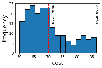
(a) ABDCP-EXP

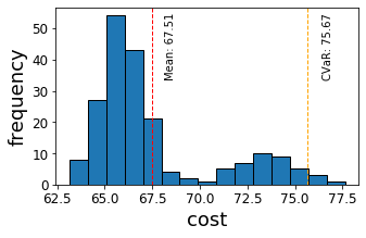
(b) ABDCP-CVaR($\alpha=0.95$)

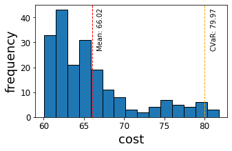
(c) ABDCP-CVaR($\alpha=0.8$)

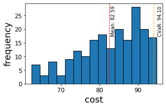
(d) Nominal

Figure 1: Histogram of the actual performance over 200 replications for different algorithms. Number of data points is set to $N=10$.

BR-MDP hedges against epistemic uncertainty: in each replication, data points are randomly sampled from the true distribution. While facing the epistemic uncertainty, BR-MDP formulation optimizes over a dynamic risk measure that provides robustness. Table 1 shows that our proposed ABDCP algorithm is the most robust in the sense of balancing the mean and variability of the actual cost. The CVaR cost of our proposed algorithm is also lower than the other benchmarks, showing that it avoids large costs. In contrast, the nominal approach performs badly when the data size is small, e.g. $N=5$, indicating that it is not robust against the epistemic uncertainty and suffers from the scarcity of data. On the other hand, DR-MDP is overly conservative, even though it has the smallest variability. This conservativeness comes from two aspects. First, it always chooses to optimize over the worst-case scenario, which rarely happens in the true system. Second, the static worst-case risk measure prevents it from adapting to the data realizations, which is one of the motivations for the dynamic risk measure considered in the BR-MDP formulation.

Convergence of ABDCP: the running time for a single replication on the path planning problem using our proposed ABDCP algorithm is affordable, and the proposed algorithm solves the infinite-horizon BR-MDP in finite time. In contrast, the infinite-horizon BR-MDP is intractable with standard value iteration or policy iteration.

5 Conclusions

In this paper, we consider the offline planning problem in MDPs with epistemic uncertainty, where we only have access to a prior belief distribution over MDPs that is constructed by the offline data. We consider the infinite-horizon BR-MDP that produces a time-consistent formulation and provides the robustness against epistemic uncertainty. We develop an efficient optimization-based approximation algorithm that converges to the optimal policy. Our experiment results demonstrate the efficiency of the proposed approximate algorithm, and show the robustness and the adaptivity to future data realization of the infinite-horizon BR-MDP formulation.

One of the future directions is to study the sample complexity of the proposed algorithm. In its current form, we show the convergence of the proposed algorithm without analysis of the convergence rate. Another interesting direction is to utilize function approximation to improve the scalability of the proposed approach to more complex domains. Separate encoders for the physical state and belief state have been proposed in (Lee et al., 2018) to reduce the dimension of the considered BA-MDP formulation, and adaptation from the risk-neutral BA-MDP formulation to our risk averse BR-MDP formulation with the designed policy network could be interesting.

Appendix A Technical Proof

Proof of Lemma 3.2.

Note that

$$(\mathcal{T}^{\pi}V)(s,\mu)=\rho_{\mu_{1}}\mathbb{E}_{\theta_{1}}[C(s_{1},a_{1}.\xi_{1})+\gamma\rho_{\mu_{2}}\mathbb{E}_{\theta_{2}}[C(s_{2},a_{2},\xi_{2})+\cdots+\gamma V(s_{k},\mu_{k})]]$$

for all positive integer $k$. As the terminal value function $V(s_{k},\mu_{k})\leq V^{\prime}(s_{k},\mu_{k})$ for all $s_{k}\in\mathcal{S},\mu_{k}\in\mathcal{M}$, and using the monotonicity of the convex risk measure $\rho(X)\leq\rho(Y)$ if $X(\omega)\leq Y(\omega),\forall\omega\in\Omega$, we have $(\mathcal{T}^{\pi}V)(s,\mu)\leq(\mathcal{T}^{\pi}V^{\prime})(s,\mu)$. Same analysis works for operator $\mathcal{T}$. ∎

Proof of Lemma 3.3.

Let $C_{\max}=\max_{s\in\mathcal{S},\mu\in\mathcal{M}}|V(s,\mu)-V^{\prime}(s,\mu)|$, we have

$$V(s,\mu)-C_{\max}\leq V^{\prime}(s,\mu)\leq V(s,\mu)+C_{\max}$$ (7)

Applying $\mathcal{T}^{\pi}$ on inequality (7), we have

$$(\mathcal{T}^{\pi}V)(s,\mu)-\gamma C_{\max}\leq(\mathcal{T}^{\pi}V^{\prime})(s,\mu)\leq(\mathcal{T}^{\pi}V)(s,\mu)+\gamma C_{\max},$$

which is justified by the translation invariance of the convex risk measure. Then we have

$$\max_{s\in\mathcal{S},\mu\in\mathcal{M}}|(\mathcal{T}^{\pi}V)(s,\mu)-(\mathcal{T}^{\pi}V^{\prime})(s,\mu)|\leq\gamma\max_{s\in\mathcal{S},\mu\in\mathcal{M}}|V(s,\mu)-V^{\prime}(s,\mu)|,$$

i.e., $||\mathcal{T}^{\pi}V-\mathcal{T}^{\pi}V^{\prime}||_{\infty}\leq\gamma||V-V^{\prime}||_{\infty}$. Same analysis works for operator $\mathcal{T}$. ∎

Proof of Proposition 3.4.

(i) Let $\pi$ be the policy for which

$$V\geq\mathcal{T}^{\pi}V.$$ (8)

Note that such policy exists as one can choose $\pi$ that yields low current cost. Applying operator $\mathcal{T}^{\pi}V$ to both sides of inequality (8) and using Lemma 3.2, we have $V\geq(\mathcal{T}^{\pi})^{t}V$, $t=1,2,\cdots$. Note that the right hand side of the above inequality represents the cost of a finite horizon problem with stationary policy $\pi$ and with final value function $V$. Also note that

$$(\mathcal{T}^{\pi})^{t}V =\rho_{\mu_{1}}\mathbb{E}_{\theta_{1}}[C(s_{1},a_{1},\xi_{1})+\cdots+\gamma V(s_{t+1},\mu_{t+1})]$$

$$\geq\rho_{\mu_{1}}\mathbb{E}_{\theta_{1}}[C(s_{1},a_{1},\xi_{1})+\cdots+\gamma\rho_{\mu_{t}}\mathbb{E}_{\theta_{t}}[C(s_{t},a_{t},\xi_{t})]].$$

Let $t\to\infty$, we get $V\geq V^{\pi}$, where $V^{\pi}$ is the value function under policy $\pi$. Since $V^{*}=\min_{\pi}V^{\pi}$, we have $V\geq V^{*}$.

(ii) Consider an arbitrary policy $\pi$ and a finite horizon problem with terminal cost $V(s_{t+1},\mu_{t+1})$. We have under the policy $\pi$,

$$\rho_{\mu_{1}}\mathbb{E}_{\theta_{1}}[C(s_{1},a_{1},\xi_{1})+\cdots+\gamma V(s_{t+1},\mu_{t+1})]=\rho_{\mu_{1}}\mathbb{E}_{\theta_{1}}[C(s_{1},a_{1},\xi_{1})+\cdots+\gamma\rho_{\mu_{t}}\mathbb{E}_{\theta_{t}}[C(s_{t},a_{t},\xi_{t})+\gamma V(s_{t+1},\mu_{t+1})]].$$

Note that $\rho_{\mu_{t}}\mathbb{E}_{\theta_{t}}[C(s_{t},a_{t},\xi_{t})+\gamma V(s_{t+1},\mu_{t+1})]\geq\mathcal{T}V(s_{t},\mu_{t})\geq V(s_{t},\mu_{t})$. Therefore, we have

$$\rho_{\mu_{1}}\mathbb{E}_{\theta_{1}}[C(s_{1},a_{1},\xi_{1})+\cdots+\gamma V(s_{t+1},\mu_{t+1})]\geq\rho_{\mu_{1}}\mathbb{E}_{\theta_{1}}[C(s_{1},a_{1},\xi_{1})+\cdots+\rho_{\mu_{t-1}}\mathbb{E}_{\theta_{t-1}}[C(s_{t-1},a_{t-1},\xi_{t-1})+\gamma V(s_{t},\mu_{t})]].$$

Continuing, we have

$$\rho_{\mu_{1}}\mathbb{E}_{\theta_{1}}[C(s_{1},a_{1},\xi_{1})+\cdots+\gamma V(s_{t+1},\mu_{t+1})]\geq V(s,\mu).$$

Let $C_{\max}$ be an upper bound on $|V(s,\mu)|,\forall s\in\mathcal{S},\mu\in\mathcal{M}$, we have

$$\rho_{\mu_{1}}\mathbb{E}_{\theta_{1}}[C(s_{1},a_{1},\xi_{1})+\cdots+\gamma\rho_{\mu_{t}}\mathbb{E}_{\theta_{t}}[C(s_{t},a_{t},\xi_{t})]]\geq V(s,\mu)-C_{\max}\gamma^{t}.$$

Passing to the limit $t\to\infty$, we have for any policy $\pi$, $V^{\pi}(s,\mu)\geq V(s,\mu)$. Therefore, the infimum over all policy $\pi$ is bounded from below by $V(s,\mu)$, i.e., $V^{*}\geq V$. ∎

Proof of Theorem 3.6.

We first show $V^{\pi}(s,\mu)$ is concave in $\mu$ for any policy $\pi$. Note that

$$V^{\pi}(s,\mu)=\min_{\phi}\mathbb{E}_{\mu}[\Psi(\mathbb{E}_{\theta}[C(s,a,\xi)+\gamma V^{\pi}(s^{\prime},\mu^{\prime})],\phi)].$$

For $0\leq t\leq 1$ and any $\mu_{1},\mu_{2}\in\mathcal{M}$,

$$V^{\pi}(s,t\mu_{1}+(1-t)\mu_{2})$$

$$= \min_{\phi}\mathbb{E}_{t\mu_{1}+(1-t)\mu_{2}}[\Psi(\mathbb{E}_{\theta}[C(s,a,\xi)+\gamma V^{\pi}(s^{\prime},\mu^{\prime})],\phi)]$$

$$= \min_{\phi}\{\mathbb{E}_{\mu_{1}}[\Psi(\mathbb{E}_{\theta}[C(s,a,\xi)+\gamma V^{\pi}(s^{\prime},\mu^{\prime})],\phi)]+(1-t)\mathbb{E}_{\mu_{2}}[\Psi(\mathbb{E}_{\theta}[C(s,a,\xi)+\gamma V^{\pi}(s^{\prime},\mu^{\prime})],\phi)]\}$$

$$\geq t\min_{\phi_{1}}\{\mathbb{E}_{\mu_{1}}[\Psi(\mathbb{E}_{\theta}[C(s,a,\xi)+\gamma V^{\pi}(s^{\prime},\mu^{\prime})],\phi_{1})]\}+(1-t)\min_{\phi_{2}}\{\mathbb{E}_{\mu_{2}}[\Psi(\mathbb{E}_{\theta}[C(s,a,\xi)+\gamma V^{\pi}(s^{\prime},\mu^{\prime})],\phi_{2})]\}$$

$$= tV^{\pi}(s,\mu_{1})+(1-t)V^{\pi}(s,\mu_{2}).$$

The same analysis works for the optimal value function $V^{*}$. Consider running Algorithm 1 with posterior set $\hat{\mathcal{M}}$ and the entire posterior set $\mathcal{M}$. Now applying Jensen’s inequality and by Theorem 12 in (Hauskrecht, 2000), we have $\hat{V}^{*}\leq V^{*}$. Note that originally in (Hauskrecht, 2000), the proof is based on the fact that value function in partially observable Markov decision process is convex in belief and the linear programming formulation has constraint $V(b)\geq R(s,a)+\gamma\sum_{b^{\prime}}P(b^{\prime}|b,a)V(b^{\prime})$, where $R$ is the reward function. Since $V$ is convex and by linear interpolation, applying Jensen’s inequality to the right hand side of the constraint leads to $\hat{V}(b)$ greater than $V(b)$. Now we are in an opposite direction, by Jensen’s inequality and concavity of $V$, we have $\hat{V}^{*}\leq V^{*}$. ∎

Proof of Theorem 3.7.

First we show Algorithm 3 terminates in finite time. Suppose not, i.e., $\hat{V}^{\hat{\pi}^{*}}(s_{1},\mu_{1})-\hat{V}^{*}(s_{1},\mu_{1})>\epsilon$. As the number of iterations increases, $\hat{\mathcal{M}}$ will contain an increasing number of reachable posterior distributions, since Algorithm 3 is guaranteed to generate new reachable posterior distributions unless the current approximate optimal policy $\hat{\pi}^{*}$ is evaluated accurately. As the number of iterations goes to infinity, $\hat{\mathcal{M}}$ will eventually contain enough posterior distributions to accurately evaluate all policies $\hat{\pi}^{*}$ that Algorithm 3 produces infinitely often. Since Algorithm 3 terminates as soon as Algorithm 1 produces a policy that is evaluated accurately, we reach a contradiction.

Nest we show the algorithm converges to $V^{*}$. Suppose that the algorithm terminates, but it converges to a suboptimal policy $\tilde{\pi}$. By Theorem 3.6, we know that $\hat{V}^{*}\leq V^{*}$, since $V^{*}\leq\hat{V}^{\tilde{\pi}}$ and the algorithm terminates when $\hat{V}^{\tilde{\pi}}-\hat{V}^{*}\leq\epsilon$. Then we have $\hat{V}^{\tilde{\pi}}-V^{*}\leq\epsilon$, which reaches a contradiction. Thus the algorithm must converge to $V^{*}$. ∎

Appendix B Implementation Details

B.1 Offline Path Planning

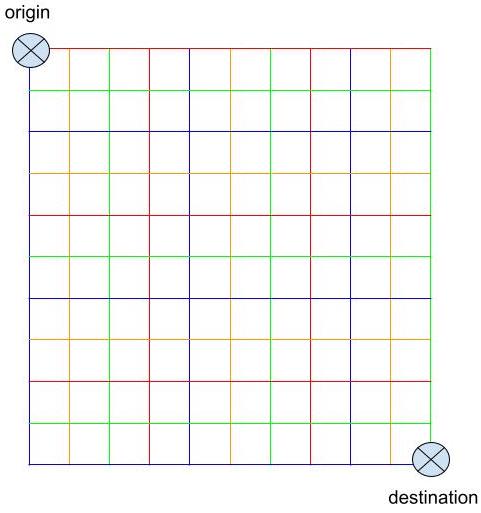
Figure 2: Path planning terrain map. Colors indicate the road types as follows–blue: highway, red: main road, orange: street, green: lane.

An autonomous car (agent) navigates a two-dimensional terrain map represented by a 10 by 10 grid along roads to the destination, as shown in Figure 2. The agent chooses from four actions {up, down, left, right}, as long it remains on the road. There are four types of roads: {highway, main road, street, lane}. The traffic time $\xi^{T}_{i}$ in each type of road is assumed to be independent and follows exponential distribution with different rate, denoted by $\theta_{i}^{T},i=1,\cdots,4$, where $T$ stands for traffic time. Specifically, the true rates are $\theta_{1}^{T}=1$, $\theta_{2}^{T}=0.5$, $\theta_{3}^{T}=0.2$, and $\theta_{4}^{T}=0.1$ but unknown to the agent. We view the parameter as a random variable, whose value is assumed to be within the following finite set $\{0.05,0.1,0.2,0.25,0.3,0.4,0.5,0.6,0.7,0.8,0.9,1,1.5,2,2.5\}$. $\xi_{i}^{A}\in\{0,1\},i=1,\cdots,4$ denotes whether there is car accident in each type of road, where $A$ stands for accident. The probability of car accident happening in each type of road is also assumed to be independent, denoted by $\theta_{i}^{A}$. Specifically, the true probabilities are $\theta_{1}^{A}=0.3$, $\theta_{1}^{A}=0.2$, $\theta_{1}^{A}=0.1$ and $\theta_{1}^{A}=0.05$ but unknown to the agent. We view the parameter as a random variable, whose value is assumed to be within the following finite set $\{0.05,0.1,0.15,0.2,0.25,0.3,0.35,0.4,0.45,0.5\}$. When there is an car accident, the agent receives a constant cost $T_{A}=10$ and makes no transition. Otherwise, the agent transitions to the next road depending on the action it takes and receives the cost, which is the traffic time for traversing that type of road. The agent stops when it reaches the destination. The discount factor $\gamma=0.95$. The agent is given a historical dataset $\mathcal{H}_{0}$ of size $N$ containing past traffic times and car accident logs, and uses the given dataset to construct the prior for the transition rate and probability of car accident. Other parameters are as follows: number of points to be added at each iteration $n=20$, threshold $\epsilon=0.1$.

B.2 Multi-item Inventory Control

The warehouse manager (agent) decides how much to replenish from the set $\{0,1,\cdots,S_{i}-s_{i}\}$ for each item $i\in[K]$ at each time stage, where $K=5$ is the number of different items, $S_{i}=100$ is the storage capacity for each item $i$, $s_{i}$ is the current inventory level for each item $i$. The customer demand is a random vector $\xi=(\xi^{1},\cdots,\xi^{K})$ with each $\xi_{i}$ following a Poisson distribution with parameter $\theta^{i}$. The true parameter is $\theta^{1}=10$, $\theta^{2}=15$, $\theta^{3}=20$, $\theta^{4}=25$, and $\theta^{5}=30$ but unknown to the agent. We view the parameter as a random variable, whose value is assumed to be within the following finite set $\{5,6,7,\cdots,33,34,35\}$. The state transition is given by $s_{t+1}=\max(s_{t}+a_{t}-\xi_{t},0)$, where $a_{t}$ is the amount of inventory to be replenished. Inventory level is not allowed to drop below zero (no backlog). When the customer demand is higher than the supply, there is a penalty cost $p$ for each unit of unsatisfied demand. When the customer is lower than the supply, there is a holding cost $h$ for each unit of overstock. In particular, for different items, $p_{1}=4$, $p_{2}=5$, $p_{3}=6$, $p_{4}=7$, $p_{5}=8$, $h_{1}=2$, $h_{2}=3$, $h_{3}=4$, $h_{4}=5$, $h_{5}=6$. The cost function at each stage is then given by $C(s_{t},a_{t},\xi_{t})=h^{T}\cdot\max(s_{t}+a_{t}-\xi_{t},0)+p^{T}\cdot\max(\xi_{t}-s_{t}-a_{t},0)$. The discount factor $\gamma=0.95$. The agent starts with 0 inventory and is given a historical dataset $\mathcal{H}_{0}$ of size $N$ containing past customer demands for different items, and uses the given dataset to construct the prior for the rate parameter. Other parameters are as follows: number of points to be added at each iteration $n=20$, threshold $\epsilon=0.1$.

B.3 DR-MDP Details

The DR-MDP approach, or Distributionally Robust Markov Decision Process, is a method for decision making under uncertainty where the ambiguity set, or the set of possible distributions for the uncertain parameters, is constructed using prior knowledge about the probabilistic information. However, this prior knowledge is not always readily available from a given data set, making the construction of the ambiguity set difficult in some cases.

We note that the Bayesian Risk Optimization (BRO) approach has a distributionally robust optimization (DRO) interpretation. In particular, for a static stochastic optimization problem, it has been shown in (Wu et al., 2018) that the BRO formulation with the risk functional taken as Value-at-Risk (VaR) with a confidence level of $100\%$ is equivalent to a DRO formulation with the ambiguity set constructed for the uncertain parameter, $\theta$. This means that BRO and DRO can be used interchangeably, depending on the problem at hand and the level of uncertainty and prior knowledge about the parameters. Therefore, for a given problem when prior knowledge about the probabilistic information is not readily available, we adapt DR-MDP to our considered problem as follows: we use samples of the uncertain parameter, $\theta$, drawn from the posterior distribution computed from a given data set. This allows us to construct an ambiguity set for $\theta$ using the available data, instead of relying on prior knowledge. Once we have samples of $\theta$, we can obtain the optimal policy that minimizes the total expected cost under the most adversarial $\theta$ among the samples.

B.4 Bilevel Optimization

We show the bilevel DCP can be reduced to a single-level DCP. Specifically, we show this transformation for the exact bilevel DCP in (4), and the same technique can be applied to the approximate algorithm.

Consider a general bilevel optimization problem:

$$\min_{x_{u},x_{l}}F(x_{u},x_{l})$$ (9)

$$\text{s.t. }x_{l}\in\operatorname*{arg\,min}_{x_{l}}\{f(x_{u},x_{l}):g(x_{u},x_{l})\leq 0\}$$

$$~{}~{}~{}~{}~{}~{}G(x_{u},x_{l})\leq 0$$

where $x_{u}$ is the upper-level variable, $x_{l}$ is the lower-level variable, $G$ denotes the upper-level constraints, $g$ denotes the lower-level constraints, $F$ denotes the upper-level objective function, $f$ denotes the lower-level objective function. The Karush-Kuhn-Tucker (KKT) conditions are a set of necessary and sufficient conditions for a solution to be optimal in a convex optimization problem. When the lower-level problem in a bilevel optimization problem is convex and sufficiently regular, the KKT conditions can be used to reformulate the problem as a single-level constrained optimization problem, which is typically easier to solve. The general bilevel optimization problem 9 can then be reduced to the following single-level optimization:

$$\min_{x_{u},x_{l}}F(x_{u},x_{l})$$

$$\text{s.t. }G(x_{u},x_{l})\leq 0$$

$$~{}~{}~{}~{}~{}~{}\nabla_{x_{l}}L(x_{u},x_{l},\lambda)=0$$

$$~{}~{}~{}~{}~{}~{}g(x_{u},x_{l})\leq 0$$

$$~{}~{}~{}~{}~{}~{}\lambda g(x_{u},x_{l})=0$$

$$~{}~{}~{}~{}~{}~{}\lambda\geq 0$$

where $L(x_{u},x_{l},\lambda)=f(x_{u},x_{l})+\lambda g(x_{u},x_{l})$ is the Lagrangian function. In the bilevel DCP (4), $V$ is the upper-level variable and $\phi$ is the lower-level variable. The constraint in (4) can be rewritten as:

$$\phi\in\operatorname*{arg\,min}_{\phi\in\Phi}\mathbb{E}_{\mu}[\Psi(\mathbb{E}_{\theta}[C(s,a,\xi)+\gamma V(s^{\prime},\mu^{\prime})],\phi)]$$

$$V(s,\mu)-\mathbb{E}_{\mu}[\Psi(\mathbb{E}_{\theta}[C(s,a,\xi)+\gamma V(s^{\prime},\mu^{\prime})],\phi)]\leq 0.$$

Since the lower-level problem is convex, we can reformulate the bilevel DCP (4) as a single-level DCP problem.

$$\min_{V}-\sum_{s\in\mathcal{S},\mu\in\mathcal{M}}\alpha(s,\mu)V(s,\mu)$$

$$\text{s.t.}V(s,\mu)-\mathbb{E}_{\mu}[\Psi(\mathbb{E}_{\theta}[C(s,a,\xi)+\gamma V(s^{\prime},\mu^{\prime})],\phi)]\leq 0$$

$$~{}~{}~{}~{}~{}\nabla_{\phi}\mathbb{E}_{\mu}[\Psi(\mathbb{E}_{\theta}[C(s,a,\xi)+\gamma V(s^{\prime},\mu^{\prime})],\phi)]=0$$

$$~{}~{}~{}~{}~{}~{}\forall a\in\mathcal{A},s\in\mathcal{S},\mu\in\mathcal{M}.$$

B.5 Additional Observations

We show additional observations for the path planning problem on Table 1 and Table 2.

Larger data size reduces epistemic uncertainty: when there are more data, the posterior distribution used in BR-MDP formulation and the MLE estimator used in the nominal approach converges to the true parameter, which reduces to solving an MDP with known transition probability and cost function. Therefore, the optimal policies and the actual costs tend to be the same.

Effect of risk measures: although both risk measures (expectation and CVaR) result in time-consistent optimal policy for each considered formulation, they provide different levels of robustness. Even though the expectation case is faster to compute, it provides the least robustness, especially when the data size is small. For the CVaR risk measure, different risk level $\alpha$ also affects the robustness. As $\alpha$ increases, the agent is more risk-averse, and the CVaR cost is smaller since it avoids more severe costs, as is shown in Figure 1(b) and Figure 1(c). But this comes with a price: its expected cost is higher. It is intuitive: even though the agent avoids severe costs, it also forfeits a chance to traverse a path that is likely to have less traffic, even though the likelihood is small. This is shown as a right-shift of the actual performance distribution from Figure 1(c) and Figure 1(b).

References

- Ahmadi et al. (2021) Ahmadi, M., Rosolia, U., Ingham, M. D., Murray, R. M., and Ames, A. D. Constrained risk-averse Markov decision processes. In Proceedings of the AAAI Conference on Artificial Intelligence, volume 35, pp. 11718–11725, 2021.
- Alagoz et al. (2015) Alagoz, O., Ayvaci, M. U., and Linderoth, J. T. Optimally solving markov decision processes with total expected discounted reward function: Linear programming revisited. Computers Industrial Engineering, 87:311–316, 2015.
- Chow & Ghavamzadeh (2014) Chow, Y. and Ghavamzadeh, M. Algorithms for CVaR optimization in MDPs. In Ghahramani, Z., Welling, M., Cortes, C., Lawrence, N. D., and Weinberger, K. Q. (eds.), Advances in Neural Information Processing Systems, 2014.
- Chow et al. (2015) Chow, Y., Tamar, A., Mannor, S., and Pavone, M. Risk-sensitive and robust decision-making: a CVaR optimization approach. In Cortes, C., Lee, D. D., Sugiyama, M., and Garnett, R. (eds.), Advances in Neural Information Processing Systems, 2015.
- Delage & Mannor (2010) Delage, E. and Mannor, S. Percentile optimization for Markov decision processes with parameter uncertainty. Operations research, 58(1):203–213, 2010.
- Duff (2002) Duff, M. O. Optimal Learning: Computational procedures for Bayes-adaptive Markov decision processes. Ph.D. diss., University of Massachusetts Amherst, 2002.
- Föllmer & Schied (2002) Föllmer, H. and Schied, A. Convex measures of risk and trading constraints. Finance and stochastics, 6(4):429–447, 2002.
- Guigues et al. (2021) Guigues, V., Shapiro, A., and Cheng, Y. Risk-averse stochastic optimal control: an efficiently computable statistical upper bound. arXiv preprint arXiv:2112.09757, 2021.
- Hansen (2013) Hansen, E. A. Solving POMDPs by searching in policy space. arXiv preprint arXiv:1301.7380, 2013.
- Hauskrecht (2000) Hauskrecht, M. Value-function approximations for partially observable Markov decision processes. Journal of artificial intelligence research, 13:33–94, 2000.
- Horst & Thoai (1999) Horst, R. and Thoai, N. V. DC programming: overview. Journal of Optimization Theory and Applications, 103(1):1–43, 1999.
- Howard & Matheson (1972) Howard, R. A. and Matheson, J. E. Risk-sensitive Markov decision processes. Management science, 18(7):356–369, 1972.
- Iyengar (2005) Iyengar, G. N. Robust dynamic programming. Mathematics of Operations Research, 30(2):257–280, 2005.
- Lee et al. (2018) Lee, G., Hou, B., Mandalika, A., Lee, J., Choudhury, S., and Srinivasa, S. S. Bayesian policy optimization for model uncertainty. arXiv preprint arXiv:1810.01014, 2018.
- Lin et al. (2022) Lin, Y., Ren, Y., and Zhou, E. Bayesian risk Markov decision processes. In Advances in Neural Information Processing Systems, 2022.
- Lipp & Boyd (2016) Lipp, T. and Boyd, S. Variations and extension of the convex–concave procedure. Optimization and Engineering, 17(2):263–287, 2016.
- Mannor & Xu (2019) Mannor, S. and Xu, H. Data-driven methods for Markov decision problems with parameter uncertainty. In Operations Research & Management Science in the Age of Analytics, pp. 101–129. INFORMS, 2019.
- Nilim & Ghaoui (2004) Nilim, A. and Ghaoui, L. Robustness in Markov decision problems with uncertain transition matrices. In Thrun, S., Saul, L., and Schölkopf, B. (eds.), Advances in Neural Information Processing Systems, 2004.
- Osogami (2012) Osogami, T. Robustness and risk-sensitivity in Markov decision processes. In Pereira, F., Burges, C. J. C., Bottou, L., and Weinberger, K. Q. (eds.), Advances in Neural Information Processing Systems, 2012.
- Petrik & Russel (2019) Petrik, M. and Russel, R. H. Beyond confidence regions: Tight Bayesian ambiguity sets for robust mdps. In Wallach, H., Larochelle, H., Beygelzimer, A., d'Alché-Buc, F., Fox, E., and Garnett, R. (eds.), Advances in Neural Information Processing Systems, volume 32, 2019.
- Petrik & Subramanian (2012) Petrik, M. and Subramanian, D. An approximate solution method for large risk-averse Markov decision processes. In de Freitas, N. and Murphy, K. (eds.), Proceedings of the Twenty-Eighth Conference on Uncertainty in Artificial Intelligence, pp. 805–814, 2012.
- Pineau et al. (2003) Pineau, J., Gordon, G., Thrun, S., et al. Point-based value iteration: An anytime algorithm for POMDPs. In IJCAI, volume 3, pp. 1025–1032, 2003.
- Poupart et al. (2006) Poupart, P., Vlassis, N., Hoey, J., and Regan, K. An analytic solution to discrete Bayesian reinforcement learning. In Proceedings of the 23rd International Conference on Machine Learning, pp. 697–704, 2006.
- Poupart et al. (2015) Poupart, P., Malhotra, A., Pei, P., Kim, K.-E., Goh, B., and Bowling, M. Approximate linear programming for constrained partially observable Markov decision processes. In Proceedings of the AAAI Conference on Artificial Intelligence, volume 29, 2015.
- Puterman (2014) Puterman, M. L. Markov decision processes: discrete stochastic dynamic programming. John Wiley & Sons, 2014.
- Rigter et al. (2021) Rigter, M., Lacerda, B., and Hawes, N. Risk-averse bayes-adaptive reinforcement learning. In Ranzato, M., Beygelzimer, A., Dauphin, Y., Liang, P., and Vaughan, J. W. (eds.), Advances in Neural Information Processing Systems, pp. 1142–1154, 2021.
- Rockafellar & Uryasev (2000) Rockafellar, R. T. and Uryasev, S. Optimization of conditional value-at-risk. Journal of Risk, 2:21–41, 2000.
- Ruszczyński (2010) Ruszczyński, A. Risk-averse dynamic programming for Markov decision processes. Mathematical programming, 125(2):235–261, 2010.
- Shapiro (2021) Shapiro, A. Tutorial on risk neutral, distributionally robust and risk averse multistage stochastic programming. European Journal of Operational Research, 288(1):1–13, 2021.
- Shapiro et al. (2021) Shapiro, A., Dentcheva, D., and Ruszczynski, A. Lectures on stochastic programming: modeling and theory. SIAM, 2021.
- Sharma et al. (2019) Sharma, A., Harrison, J., Tsao, M., and Pavone, M. Robust and adaptive planning under model uncertainty. In Akshat Kumar, Sylvie Thiébaux, P. V. and Yeoh, W. (eds.), Proceedings of the 29th International Conference on Automated Planning and Scheduling, pp. 410–418, 2019.
- Shen et al. (2016) Shen, X., Diamond, S., Gu, Y., and Boyd, S. Disciplined convex-concave programming. In 2016 IEEE 55th Conference on Decision and Control (CDC), pp. 1009–1014. IEEE, 2016.
- Tamar et al. (2015a) Tamar, A., Chow, Y., Ghavamzadeh, M., and Mannor, S. Policy gradient for coherent risk measures. In Cortes, C., Lee, D. D., Sugiyama, M., and Garnett, R. (eds.), Advances in Neural Information Processing Systems, 2015a.
- Tamar et al. (2015b) Tamar, A., Glassner, Y., and Mannor, S. Optimizing the CVaR via sampling. In Twenty-Ninth AAAI Conference on Artificial Intelligence, 2015b.
- Wiesemann et al. (2013) Wiesemann, W., Kuhn, D., and Rustem, B. Robust Markov decision processes. Mathematics of Operations Research, 38(1):153–183, 2013.
- Wu et al. (2018) Wu, D., Zhu, H., and Zhou, E. A Bayesian risk approach to data-driven stochastic optimization: Formulations and asymptotics. SIAM Journal on Optimization, 28(2):1588–1612, 2018.
- Xu & Mannor (2010) Xu, H. and Mannor, S. Distributionally robust Markov decision processes. In Lafferty, J., Williams, C., Shawe-Taylor, J., Zemel, R., and Culotta, A. (eds.), Advances in Neural Information Processing Systems, 2010.
- Zhou & Xie (2015) Zhou, E. and Xie, W. Simulation optimization when facing input uncertainty. In Yilmaz, L., Chan, W. K. V., Moon, I., Roeder, T. M. K., Macal, C., and Rossetti, M. D. (eds.), Proceedings of the 2015 Winter Simulation Conference, pp. 3714–3724, 2015.