FedHQL: Federated Heterogeneous Q-Learning

Abstract

Federated Reinforcement Learning (FedRL) encourages distributed agents to learn collectively from each other’s experience to improve their performance without exchanging their raw trajectories. The existing work on FedRL assumes that all participating agents are homogeneous, which requires all agents to share the same policy parameterization (e.g., network architectures and training configurations). However, in real-world applications, agents are often in disagreement about the architecture and the parameters, possibly also because of disparate computational budgets. Because homogeneity is not given in practice, we introduce the problem setting of Federated Reinforcement Learning with Heterogeneous And bLack-box agEnts (FedRL-HALE). We present the unique challenges this new setting poses and propose the Federated Heterogeneous Q-Learning (FedHQL) algorithm that principally addresses these challenges. We empirically demonstrate the efficacy of FedHQL in boosting the sample efficiency of heterogeneous agents with distinct policy parameterization using standard RL tasks.

1 Introduction

Leveraging on the growing literature of federated learning (FL) (McMahan et al., 2017; Konečnỳ et al., 2016; Kairouz et al., 2021, etc.), federated reinforcement learning (FedRL) (Zhuo et al., 2019) has recently become an emerging approach to enable collective intelligence (Yahya et al., 2017) in sequential decision-making problems with a large number of distributed reinforcement learning (RL) agents. In contrast to the conventional setting of distributed RL in which the raw trajectories of agent-environment interactions may be collected by a central server (Nair et al., 2015; Mnih et al., 2016; Espeholt et al., 2018; Horgan et al., 2018; Chen et al., 2022, etc.), FedRL, as a specialization of distributed RL, places its emphasis on the accessibility of the raw trajectories of agents in real-world domains such as e-commerce and healthcare. For example, in the healthcare domain, sharing trajectories corresponding to the medical records of patients is prohibitive (Rieke et al., 2020). Thus, applications like the clinical decision support system proposed by Xue et al. (2021) need to utilize FedRL to extract knowledge from electronic medical records from distributed sources where the raw records are inaccessible directly. FedRL may also be applied to practical applications where transmitting RL trajectories is infeasible due to limited hardware capacities and transmission bandwidth. For instance, Liu et al. (2019) develops a FedRL server in the cloud for a group of robots to learn to navigate cooperatively through the world without transmitting their observation trajectories to the server to save bandwidth. Besides those promising practical applications, many endeavors have been made to study the theoretical aspects of FedRL. For example, FedRL has recently been theoretically proved to be effective in improving the sample efficiency of RL agents proportionally with respect to the number of agents with performance guarantees (Fan et al., 2021); the work of Jin et al. (2022) has proved the convergence of FedRL algorithms with agents operating in distributed environments with different state-transition dynamics; Khodadadian et al. (2022) has further proved that FedRL can provide a linear convergence speedup with respect to the number of agents under Markovian noise.

Despite their promising theoretical results (Fan et al., 2021; Jin et al., 2022; Khodadadian et al., 2022) and practical applications (Nadiger et al., 2019; Liu et al., 2019; Yu et al., 2020; Wang et al., 2020; Fujita et al., 2022; Liang et al., 2023), current FedRL algorithms explicitly assume that all participants are homogeneous, which requires all agents to share the same policy parameterization (e.g., the architecture of the policy neural network, including the number of layers, the activation function, etc.) and the same training configurations for the policy (e.g., the learning rate). Such an assumption can be a significant limitation in real-world applications where agents are often heterogeneous, due to various factors such as different computational budgets, different assessments of the difficulty of the task, etc. To solve this problem, we propose a federated version of Q-learning (Watkins, 1989) that works with $N$ distributed agents that are heterogeneous in terms of a number of factors including the policy parameterization (e.g., the policy network architecture), the policy training configurations (e.g., the learning rate) and the exploration strategy to manage the trade-off between exploration and exploitation.

Another important issue faced by existing FedRL algorithms results from the assumption that the server has full knowledge about the policy-related details of agents, which is a privacy concern to the agents. In the aforementioned previous works on FedRL, the server has access to information such as the architectures of the policy networks, the details on how the agents train and update their policy networks, and the exploration strategy of the agents to trade off exploration and exploitation. Such information may reveal critical information about the agents. For example, consider a FedRL application in the financial market where the agents are different organizations. Knowing that one organization utilizes a computationally expensive transformer network (Chen et al., 2021) may imply the organization’s relations with customers and excellent financial standing. To address this issue, our proposed federated Q-learning algorithm treats each agent as a black-box expert whose policy network parameterization, training configuration and exploration strategy are hidden from any other party including the server.

In this work, we propose the problem setting of Federated Reinforcement Learning with Heterogeneous And bLack-box agEnts (FedRL-HALE). In the setting of FedRL-HALE, which is illustrated in Fig. 1, every agent is free to choose its own preferred policy parameterization, training configurations, and exploration strategy. Furthermore, the agents in the setting of FedRL-HALE are black-box experts whose policy-related information, such as those mentioned above, is not shared with any other party including the server. To achieve collaborative learning of heterogeneous and black-box agents in the setting of FedRL-HALE, we introduce the Federated Heterogeneous Q-Learning (FedHQL) algorithm. To allow the server to aggregate information from different agents and use it to improve their learning, we propose (a) the Federated Upper Confidence Bound (FedUCB) algorithm, which is deployed by the server as a subroutine of the FedHQL algorithm, and (b) a federated version of Temporal Difference (FedTD) which is calculated by the server and then broadcast to all agents to improve their policies.

Specifically, we make the following contributions:

1. We introduce the problem formulation of FedRL-HALE and discuss its technical challenges (Sec. 3).

2. We develop the FedUCB algorithm, which provides a principled strategy for inter-agent exploration to balance the trade-off between exploration and exploitation in the setting of Fed-HBA (Sec. 4.2).

3. We propose the FedHQL algorithm, which deploys FedUCB as a subroutine and is the first FedRL algorithm catered to heterogeneous and black-box agents (Sec. 4.5).

4. We conduct extensive empirical evaluations to demonstrate the efficacy of FedHQL in improving the sample efficiency of agents using standard RL tasks (Sec. 5).

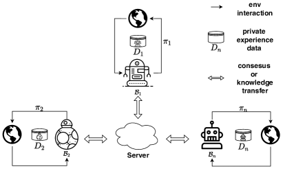
Figure 1: Graphical illustration of the FedRL-HALE problem setup (Sec. 3.1). $\mathcal{B}_{n}$ represents a black-box agent whose policy-related information and private experience data $D_{n}$ are not accessible to any other party. A central server performs certain knowledge aggregation process in order to improve the performance of participating agents without accessing the aforementioned private information of the agents.

2 Preliminaries

2.1 Markov Decision Processes

We model Reinforcement Learning (RL) as a discrete-time episodic Markov Decision Process (MDP) (Sutton & Barto, 2018): $M\triangleq\{\mathcal{S},\mathcal{A},\mathcal{P},\mathcal{R},\gamma,\rho,H\}$ where $\mathcal{S}$ and $\mathcal{A}$ are the state space and action space of the RL task, respectively. $\mathcal{P}(s^{\prime}|s,a)$ defines the transition probability of the environment, $\mathcal{R}(s,a):\mathcal{S}\times\mathcal{A}\mapsto[0,R]$ denotes the reward function, $\gamma\!\in\!(0,1)$ is the discount factor, $\rho$ represents the initial state distribution, and $H$ denotes the task horizon of an episode. An agent behaves according to its policy $\pi$, where $\pi(a|s)$ defines the probability of the agent choosing action $a$ at state $s$. $\tau\triangleq\{s_{0},a_{0},s_{1},a_{1},...,s_{H-1},a_{H-1}|s_{0}\!\sim\!\rho\}$ is a trajectory of agent-environment interactions. The return function $R_{t}\triangleq\sum_{i=0}^{H}\gamma^{i}\mathcal{R}\left(s_{t+i},a_{t+i}\right)$ gives the cumulative discounted reward from timestep $t$ in $\tau$ that an RL algorithm aims to maximize.

2.2 Q-learning

One of the most important breakthroughs in RL was the development of Q-learning (Watkins, 1989; Sutton & Barto, 2018) which launched the field of deep RL by using neural networks as function approximators (Mnih et al., 2013). The core of this model-free RL algorithm is to iteratively apply the Bellman equation to update the action-value function $Q$:

$$Q(s_{t},a_{t})\leftarrow Q (s_{t},a_{t})+\alpha\Big{[}\mathcal{R}(s_{t+1},a_{t+1})$$

$$+\gamma\max_{a}Q(s_{t+1},a)-Q(s_{t},a_{t})\Big{]}$$ (1)

where $Q(s,a)\!:\!\mathcal{S}\times\mathcal{A}\mapsto\mathbb{R}$ represents the value of an action $a$ at state $s$, and $\alpha$ is the learning rate. Then a decision policy $\pi(a_{t}|s_{t})$ can be obtained via exploiting the updated $Q$:

$$a_{t}=\arg\max_{a}Q(s_{t},a).$$ (2)

The optimal action at state $s_{t}$ is defined as $a^{*}_{t}=\arg\max_{a}Q^{*}(s_{t},a)$ where $Q^{*}(s_{t},a)$ is the optimal Q-function which gives the expected return for starting in state $s$, taking action $a$, and following the policy thereafter.

One key characteristic of Q-learning is that the optimization step is always performed off-policy meaning that each update of Eq. (2.2) can use any data samples collected at any point, regardless of how the agent deals with the exploration-exploitation dilemma (Sec. 2.3) to collect the samples.

2.3 The Exploration-Exploitation Dilemma

During the learning process, when an agent makes a decision that seems optimal according to Eq. (2), it is exploiting its current knowledge which is assumed to be reliable; the agent may also selects an action that seems sub-optimal for now to potentially explore unseen states, making the assumption that its current knowledge could be incomplete and inaccurate. This is known as the exploration-exploitation dilemma, which is omnipresent in many sequential decision-making problems. To balance the trade-off between exploration and exploitation, a variety of exploration strategies has been developed, such as $\epsilon$-greedy and Boltzmann exploration (Cesa-Bianchi et al., 2017). Among them, the $\epsilon$-greedy algorithm is widely used in Q-learning as its exploration strategy:

$$a_{t}=\begin{cases}\arg\max_{a}{Q}(s_{t},a)&\text{ with probability }1-\epsilon,\\ \text{random action }a&\text{ with probability }\epsilon\end{cases}$$

where the coefficient $\epsilon$ is a hyper-parameter that controls the degree of exploration.

One optimism-based exploration strategy is the Upper Confidence Bound (UCB) algorithms (Lattimore & Szepesvári, 2020), which is established based on the principle of optimism in the face of uncertainty. The action chosen by UCB at time step $t$ is given by:

$$a_{t}=\arg\max_{a}\Big{[}Q(s_{t},a)+c\sqrt{\frac{\log t}{N_{t}(a)}}\Big{]}$$ (3)

where $Q(s_{t},a)$ is the current estimated value of action $a$ at time step $t$; $N_{t}(a)$ is the number of times action $a$ has been selected prior to time $t$; $c$ is a confidence constant that controls the level of exploration. The UCB algorithms construct a high-probability upper bound on $Q(s_{t},a)$ and automatically balance exploration and exploitation as more knowledge of the environment is gathered.

3 FedRL-HALE

3.1 Problem formulation

Consider the task of federatively solving a sequential decision-making problem represented by the MDP $M\triangleq\{\mathcal{S},\mathcal{A},\mathcal{P},\mathcal{R},\gamma,\rho,T\}$ defined in Sec. 2.1. Let the set $\mathcal{B}\triangleq\{Q_{n}(a|\ell_{n}(s;{D}_{n},\omega_{n}))\}_{n=1}^{N}$ denote a group of $N$ distributed heterogeneous and black-box agents. Following the same setup as the existing literature of FedRL (Sec. 1), each agent $\mathcal{B}_{n}$ independently operates in a separate copy of the underlying MDP $M$ following its policy $\pi_{n}$, and generates its private experience data $D_{n}\triangleq\{(s,a,s^{\prime},r)_{i}\}_{i=1}^{|D_{n}|}$. Each action valuator $Q_{n}(a|\ell_{n}(s;{D}_{n},\omega_{n}))$ consists of a non-linear function $\ell_{n}(s;{D}_{n},\omega_{n})$ which predicts the value of action $a$ given a state $s$. The non-linear function $\ell_{n}(s;{D}_{n},\omega_{n})$ is parameterized by a set of parameters $\omega_{n}$ and learned using the private experience data ${D}_{n}$.

A prominent example of such a non-linear function $\ell_{n}$ is a neural network, in which $\omega_{n}$ represents its weights. Due to the heterogeneity among agents, different agents may choose different neural network architectures and employ different optimization methods to train their networks. For example, agent $\mathcal{B}_{1}$ favours a Transformer-like network architecture and trains it with the Adam Optimizer (Chen et al., 2021); agent $\mathcal{B}_{2}$ can choose to use a 3-layer multi-layer perceptron (MLP) as the network and train it using conventional stochastic gradient ascent; meanwhile, agent $\mathcal{B}_{3}$ who also adopts an MLP as the network may utilize an SVRG-type (Johnson & Zhang, 2013; Papini et al., 2018) optimizer for training. As aforementioned, the neural network $\ell_{n}(s;{D}_{n},\omega_{n})$ is trained on a private set of experience data $D_{n}$ for agent $\mathcal{B}_{n}$. And we note that in any given state $s$, the neural network-based action valuator $Q_{n}(a|\ell_{n}(s;{D}_{n},\omega_{n}))$ is able to predict the value of any action $a$. To simplify exposition, in the remainder of the paper, we use $Q_{n}(s,a)$ to denote the action valuator $Q_{n}(a|\ell_{n}(s;{D}_{n},\omega_{n}))$.

Similar to the settings in the existing FedRL works (Fan et al., 2021; Jin et al., 2022; Khodadadian et al., 2022), a reliable central server is available to coordinate the FedRL process and is allowed to interact with another separate copy of the underlying MDP (Fan et al., 2021). At any point during the FedRL training process, the server may query all black-box agents with a selected state $\bar{s}$, and then collect from every agent $\mathcal{B}_{n}$ the action values $Q_{n}(\bar{s},a)$ for all actions $a$’s. The server then needs to design a mechanism for aggregating the collected information and broadcasting it back to all agents to aid their individual training. Of note, the information regarding the non-linear function $\ell_{n}$ (including its architecture, weights $\omega_{n}$, training methods, and other training details), as well as the local experience data $D_{n}$, is not revealed to any other party, including the central server.

Let $R_{n}$ and $\overline{R}_{{n}}$ denote the performances achievable by agent $\mathcal{B}_{n}$ through independent learning and FedRL-HALE, respectively. Let $|D_{n}|$ and $|\overline{D}_{n}|$ denote, respectively, the number of agent-environment interactions required to reach $R_{n}$ through independent learning and to reach $\overline{R}_{n}$ through FedRL-HALE. $|\overline{D}_{s}|$ denotes the total number of interactions incurred at the server. We define two objectives in the setting of FedRL-HALE:

(1) from the perspective of improving the overall system welfare: We aim to improve the average performance of all agents, given a fixed budget on the number of interactions with the whole system:

$$\underbrace{\frac{\sum_{n}\overline{R}_{n}}{N}}_{\text{FedRL-HALE}}\geq\underbrace{\frac{\sum_{n}{R}_{n}}{N}}_{\text{self-learning}}s.t.\ \underbrace{|\overline{{D}}_{s}|+\sum_{n}|\overline{D}_{n}|}_{\text{FedRL-HALE}}\leq\underbrace{\sum_{n}|{D}_{n}|.}_{\text{self-learning}}$$ (4)

(2) from the perspective of each participating agent $\mathcal{B}_{n}$ who aims to improve its performance with less agent-environment interactions compared to that of independent learning: We aim to achieve:

$$\underbrace{|\overline{D}_{n}|}_{\text{FedRL-HALE}}\leq\underbrace{|{D_{n}}|}_{\text{self-learning}}s.t.\ \underbrace{\overline{R}_{n}}_{\text{FedRL-HALE}}\geq\underbrace{R_{n}.}_{\text{self-learning}}$$ (5)

3.2 Technical Challenges

Here we discuss unique technical challenges that arise in the above-proposed setting of FedRL-HALE.

Black-box Optimization. Since the details of policy network architecture, training configuration, and exploration strategy of every agent are not revealed to any other party including the server, it is challenging to construct and optimize the objective function of FedRL-HALE, resulting in a distributed black-box optimization problem (Bajaj et al., 2021). It is thus infeasible to solve the FedRL-HALE problem with conventional gradient-based methods (Fan et al., 2021) or parameter-based methods (Khodadadian et al., 2022) for knowledge aggregation. Meanwhile, the nature of black-box optimization renders conventional federated aggregation methods from the federated learning literature, such as federated averaging (FedAvg) (McMahan et al., 2017), inapplicable in FedRL-HALE.

To this end, we propose a federated version of Q-learning (Sec. 2.2) that aggregates the action value estimations of different agents $Q_{n}$’s on the states queried by the central server. The knowledge encoded in the aggregated action value estimation, denoted as $\bar{Q}$, is then broadcast back to every agent for its individual policy improvement.

Inter-agent Exploration. The exploration-exploitation dilemma (Sec. 2.3) requires an agent to design a principled way to balance between exploiting its current knowledge and exploring to acquire new knowledge, which we will refer to as the intra-agent exploration problem. Similarly, we note that in the setting of FedRL-HALE, the exploration-exploitation dilemma needs to be further considered when the server aggregates information from all agents, i.e., when the server selects its action to interact with the environment. This is because the actions selected by the server determine the specific state-action pairs whose value estimates $Q_{n}$’s gets improved via federation for all agents (Section 4). Therefore, a natural trade-off arises when the server selects its action: Should the server select actions by exploiting the current information provided by all agents, i.e., select actions which are deemed promising by all agents? Or should the server select exploratory actions for which the agents have inconsistent (i.e., high-variance) value estimations? This additional exploration-exploitation dilemma similarly highlights the requirement for a principled algorithm to balance the trade-off between exploiting the current knowledge of the entire group of agents and exploring to obtain new knowledge, which we will denote as inter-agent exploration.

In this paper, to design the inter-agent exploration strategy, we leverage the well-celebrated optimism-based exploration strategy of upper confidence bound (UCB) (Sec. 2.3), and develop a Federated UCB (FedUCB) algorithm which provides a principled way to balance the trade-off between exploration and exploitation when aggregating the knowledge of the group of agents.

4 FedHQL

To achieve collaborative learning of heterogeneous and black-box agents in the setting of FedRL-HALE and address its unique technical challenges (Section 3.2), we propose a novel Federated Heterogeneous Q-Learning (FedHQL) algorithm in this section. We will firstly discuss each component of FedHQL in detail and then present the overal algorithm in Sec. 4.5.

4.1 Federated Q-learning

At the core of FedHQL is the federated version of Q-learning with $N$ heterogeneous and black-box agents. Each agent $\mathcal{B}_{n}$ independently interacts with its own copy of the MDP using its preferred intra-agent exploration strategy. Each agent $\mathcal{B}_{n}$ updates its current estimation of action values $Q_{n}(s,a)$ through Q-learning as follows:

$$Q_{n}(s_{t},a_{t})\leftarrow Q_{n}(s_{t},a_{t})+\alpha_{n}[\mathcal{R}(s_{t+1},a_{t+1})$$

$$+\gamma\max_{a}Q_{n}(s_{t+1},a)-Q_{n}(s_{t},a_{t})].$$ (6)

Of note, every agent is free to choose any arbitrary policy parameterization (e.g., any policy network architecture for learning $Q_{n}$), training configurations for the policy network, and exploration strategy (e.g., Boltzmann exploration, $\epsilon$-greedy with different values of $\epsilon$, etc.).

To facilitate knowledge aggregation, we let the central server broadcast query state(s) to agents and query their estimations of the values of all actions at these candidate states (i.e., $Q_{n}(s,a),\forall a$). Then, the server can combine the knowledge of the entire group of agents by aggregating the received action value estimations $Q_{n}(s,a)$’s. As mentioned in Sec. 3.2, this aggregation step is faced with the exploration-exploitation challenge, calling for a principled inter-agent exploration strategy, which we will discuss next.

4.2 Federated Upper Confidence Bound (FedUCB)

In this section, we introduce our principled strategy for inter-agent exploration, i.e., for selecting the server actions (Section 3.2).

Let $b,c>0$ be constants. For a state $s$, after all action value estimations $Q_{n}(s,a),\forall a$ are received, we compute the following for every action $a$:

$$\bar{Q}(s,a) =\frac{1}{N}\sum_{n=1}^{N}Q_{n}(s,a),$$

$$\mathbb{V}_{s,a} =\frac{1}{N}\sum^{N}_{n=1}[\bar{Q}(s,a)-Q_{n}(s,a)]^{2},$$

$$Q^{\text{UCB}}(s,a) \triangleq\bar{Q}(s,a)+\sqrt{\frac{2c\mathbb{V}_{s,a}}{N}}+\frac{3bc}{N}.$$ (7)

After that, the FedUCB policy then chooses the action $\bar{a}$ using: $\bar{a}\leftarrow\arg\max_{a}Q^{\text{UCB}}(s,a)$. To understand the insights behind Eq. (7), let us begin with the following lemma.

Lemma 4.1 (Adapted from Theorem 1 in Audibert et al. (2009) ).

Let $X_{1},...,X_{N}$ be i.i.d. random variables taking their values in $[0,b]$. Let $\mu=\mathbb{E}[X_{1}]$ be their common expected value. Consider the empirical mean $\bar{X}_{N}$ and variance $\mathbb{V}_{N}$ defined by

$$\bar{X}_{t}=\frac{\sum_{n=1}^{N}X_{n}}{N}\text{ and }\mathbb{V}_{N}=\frac{\sum_{n=1}^{N}\left(X_{n}-\bar{X}_{N}\right)^{2}}{N}.$$ (8)

Then, for any $N\in\mathbb{N}$ and $\chi>0$, with probability at least $1-3e^{-\chi}$,

$$\left|\bar{X}_{N}-\mu\right|\leq\sqrt{\frac{2\mathbb{V}_{N}\chi}{N}}+\frac{3b\chi}{N}.$$ (9)

Lemma 4.1 has been used by variance-based UCB algorithms for multi-armed bandits, and its proof is provided in Audibert et al. (2009). Inspired by Lemma 4.1, we have the following:

Theorem 4.2.

For any $s$ and $a$, assume that $\{Q_{n}(s,a)\}^{N}_{n=1}$ are i.i.d. samples drawn from a distribution whose expectation is the optimal Q function at $s$ and $a$: $Q^{*}(s,a)$. Denote $\mu_{s,a}\triangleq\mathbb{E}[Q_{n}(s,a)]=Q^{*}(s,a)$. Also assume that $Q_{n}(s,a)\in[0,b],\forall s,a,n$. Then for any $c>0$, with probability at least $1-3e^{-c}$, we have

$$|\bar{Q}(s,a)-\mu_{s,a}|\leq\sqrt{\frac{2c\mathbb{V}_{s,a}}{N}}+\frac{3bc}{N}.$$

Proof.

The proof follows directly from Lemma 4.1 by setting $X_{n}=Q_{n}(s,a)$, $\bar{Q}(s,a)=\frac{1}{N}\sum_{n=1}^{N}Q_{n}(s,a)$, and
$\mathbb{V}_{s,a}=\frac{1}{N}\sum^{N}_{n=1}[\bar{Q}(s,a)-Q_{n}(s,a)]^{2}$. ∎

The assumption that $\{Q_{n}(s,a)\}^{N}_{n=1}$ are i.i.d. samples from a distribution whose expectation is $Q^{*}(s,a)$ is justified because every agent $\mathcal{B}_{n}$ aims to independently optimize its $Q_{n}$ such that it can estimate the optimal Q function $Q^{*}$. The assumption that $Q_{n}(s,a)\in[0,b]$ is also easily satisfied as long as the reward function is non-negative and upper-bounded. For every pair of $(s,a)$, Theorem 4.2 provides a high-probability upper bound on the difference between the aggregated action value $\bar{Q}(s,a)$ and the optimal action value, resulting in the following corollary:

Corollary 4.3 (FedUCB).

Under the same assumptions and notations as Theorem 4.2, for any $c>0$, with probability at least $1-3e^{-c}$, we have

$$\mu_{s,a}\triangleq Q^{*}(s,a)\leq Q^{\text{UCB}}(s,a)\triangleq\bar{Q}(s,a)+\sqrt{\frac{2c\mathbb{V}_{s,a}}{N}}+\frac{3bc}{N}.$$

Corollary 4.3 suggests that the optimal value of action $a$ at state $s$, $Q^{*}(s,a)$, is upper-bounded by $Q^{\text{UCB}}(s,a)$ defined in Eq. (7) with high confidence. Inspired by Corollary 4.3, we develop our practical FedUCB algorithm for the knowledge aggregation in FedRL-HALE, which firstly calculates (for any $s,a$):

$$\bar{Q}(s,a) =\frac{1}{N}\sum_{n=1}^{N}Q_{n}(s,a),$$ (10)

$${Q}^{\text{std}}(s,a) =\sqrt{\frac{1}{N}\sum_{n=1}^{N}[\bar{Q}(s,a)-Q_{n}(s,a)]^{2}},$$ (11)

$$Q^{\text{UCB}}(s,a) \simeq\underbrace{\bar{Q}(s,a)}_{\text{exploitation}}+\lambda\underbrace{Q^{\text{std}}(s,a)}_{\text{exploration}},$$ (12)

and then selects the server action by:

$$\bar{a}_{t}\leftarrow\arg\max_{a}Q^{\text{UCB}}(s_{t},a).$$ (13)

Note that the selected action $\bar{a}_{t}$ will determine the state-action pair whose value estimate $Q_{n}(s_{t},\bar{a}_{t})$ gets improved for all agents (details in Section 4.3). Therefore, the FedUCB algorithm (13) achieves both exploitation of the knowledge from all agents by preferring actions deemed promising by all agents (i.e., large $\bar{Q}(s,a)$) and exploration of those actions for which the value estimations from all agents are inconsistent (i.e., large $Q^{\text{std}}(s,a)$). The degree of exploration is controlled by the parameter $\lambda$, which we will refer to as inter-agent exploration coefficient, such that a larger $\lambda$ encourages the selection of more exploratory actions.

4.3 Federated Temporal Difference (FedTD)

With the FedUCB derived above , the server is able to optimistically select an action that leads to high returns with high probability. Inspired by Fan et al. (2021), we let the server operate in another separate copy of the underlying MDP and execute the selected action $\bar{a}$, hence generating a new sample $(s_{t},\bar{a},s_{t+1},r_{t})$. This new sample will then be used to perform a federated version of Temporal Difference (FedTD) learning, which is defined as follows:

$$\bar{Q}(s_{t},\bar{a}_{t}) \leftarrow\bar{Q}(s_{t},\bar{a}_{t})+$$

$${\alpha_{\text{s}}}\Big{(}r_{t}+\gamma\max_{b}\bar{Q}(s_{t+1},b)-\bar{Q}(s_{t},\bar{a}_{t})\Big{)}$$ (14)

where $\bar{Q}(s_{t},a_{t})$, defined in Eq. (10), represents the agents’ current estimation of the action value at time $t$, $\alpha_{\text{s}}$ is the learning rate of FedTD, and $r_{t}+\gamma\max_{b}\bar{Q}(s_{t+1},b)$ is the Temporal Difference (TD) target (Sutton & Barto, 2018). To calculate $\bar{Q}(s_{t+1},b)$ which is used in Eq. (4.3), the server sends the state $s_{t+1}$ to all agents and collects the value estimations of all actions at $s_{t+1}$ from all agents, after which $\bar{Q}(s_{t+1},b)$ can be again calculated using Eq. (10). If the action executed $\bar{a}_{t}$ is not optimal, then it gets penalized by receiving a smaller $r_{t}$. Essentially, FedTD regularizes the action selected by FedUCB, $\bar{a}_{t}$, at each time step $t$ by updating $\bar{Q}(s_{t},\bar{a}_{t})$ with TD target $r_{t}+\gamma\max_{b}\bar{Q}(s_{t+1},b)$.

At each time step, after the FedTD target (4.3) is calculated, it will be broadcast to all agents so that they can use it to update their action value estimations $Q_{n}$’s, which is discussed next.

4.4 Individual Improvement

One objective of FedRL-HALE is to improve the sample efficiency of the individual participating agents. To achieve this, after the FedTD target $\bar{Q}(s_{t},\bar{a}_{t})$ is updated following Eq. (4.3), we let the server broadcast the updated $\bar{Q}(s_{t},\bar{a}_{t})$ back to all agents. An agent $\mathcal{B}_{n}$ will then update its own action value estimation $Q_{n}$ using the following regression loss:

$$\mathcal{L}_{n}\triangleq\|\bar{Q}(s_{t},\bar{a}_{t})-Q_{n}(s_{t},\bar{a}_{t})\|^{2}$$ (15)

This loss serves as a regularizer that periodically updates agent $\mathcal{B}_{n}$’s parameter $\omega_{n}$ by

$$\omega_{n}\leftarrow\omega_{n}-\tilde{{\alpha}}_{n}\nabla\mathcal{L}_{n}$$ (16)

where $\tilde{{\alpha}}_{n}$ is a step-size hyper-parameter. This loss essentially helps the agent to improve its knowledge about action $\bar{a}_{t}$ at state $s_{t}$ using the knowledge aggregated by FedUCB and updated by FedTD. In FedHQL, each agent performs $\kappa$ steps of gradient updates in Eq. (16).

4.5 FedHQL Algorithm

Figure 2: Graphical illustration of FedHQL.

We are now ready to present the complete algorithm of FedHQL. Fig. 2 gives an illustration of FedHQL, and we describe the details of every step below. One federation round $t$ in FedHQL starts by the server broadcasting a query state $s_{t}$ to all agents:

$\bullet$  {1}⃝{2}⃝ (by Agents): At any point of FedHQL, every agent $\mathcal{B}_{n}$ independently performs self-learning according to Eq. (4.1) with any arbitrary choice of policy parameterization, training configurations, and intra-exploration strategy (step {1}⃝). When a query state $s_{t}$ is received from the server, agent $\mathcal{B}_{n}$ sends to the server $Q_{n}(s_{t},a),\forall a$, i.e., its current estimation of the action values at the query state $s_{t}$ for all actions $a$’s (step {2}⃝).

$\bullet$  {3}⃝{4}⃝{5}⃝ (by Central Server): After receiving the action value estimations from all agents, for every action $a$, the server computes $\bar{Q}(s_{t},a)$, ${Q}^{\text{std}}(s_{t},a)$, and $Q^{\text{UCB}}(s_{t},a)$ according to Eq. (10), Eq. (11), and Eq. (12) (step {3}⃝). An action $\bar{a}$ is then selected and executed by the server according to Eq. (13), which generates the sample $(s_{t},\bar{a}_{t},s_{t+1},r_{t})$ (step {4}⃝). Next, to prepare for the calculation of the FedTD target (4.3), the server broadcasts the state $s_{t+1}$ to all agents, and then receives from all agents their value estimations at the state $s_{t+1}$ for all actions, i.e., $\{Q_{n}(s_{t+1},a),\forall a\}^{N}_{n=1}$. This allows the server to calculate $\bar{Q}(s_{t+1},a),\forall a$ again using Eq. (10). Then, the server performs FedTD to update $\bar{Q}(s_{t},\bar{a}_{t})$ according to Eq. (4.3) and broadcasts the updated $\bar{Q}(s_{t},\bar{a}_{t})$ to all agents (step {5}⃝).

$\bullet$  {6}⃝ (by Agents): Whenever $\bar{Q}(s_{t},\bar{a}_{t})$ is received, agent $\mathcal{B}_{n}$ performs the individual improvement for $\kappa$ steps to update its own $Q_{n}$ according to the loss function defined in Eq. (15) and gradient updates in Eq. (16) (step {6}⃝).

This federation process ({2}⃝-{6}⃝) is repeated until $s_{t}$ is a terminal state or the maximum federation time horizon $H_{\text{fed}}$ is reached. After a federation round, every agent continues to repeat the independent self-learning (step {1}⃝) followed by the federation ({2}⃝-{6}⃝), until all the budgets for environment interactions are exhausted. Of note, the above process can be implemented in asynchronous batches using the reliable broadcast protocol from distributed computing (Chang & Maxemchuk, 1984). Due to space constraints, the pseudocode of FedHQL is deferred to Appendix A.

5 Evaluation

In this section, we empirically verify the effectiveness of the FedHQL algorithm using the classical control tasks of CartPole and LunarLander from the OpenAI gym environment (Brockman et al., 2016). We design our experiments with respect to the two objectives of FedRL-HALE (Sec. 3.1): I. Given a fixed budget on the total number of interactions with the whole system, does FedHQL improve the average performance of all agents? II. If an agent participates in the FedRL-HALE setup, does the FedHQL algorithm improve the sample efficiency of the agent with high probability?

5.1 Experimental Settings

To the best of our knowledge, this is the first FedRL algorithm that is able to aggregate knowledge from heterogeneous and black-box agents. We thus compare the performance of the agents with FedHQL and without federation (independent self-learning) which we refer to as DQN (w.o. Fed). We initialize $N=5$ heterogeneous agents and use the default implementation of classical deep Q-learning (DQN) from the stable baselines library (Raffin et al., 2021) as the backbone training algorithm for each agent.

Table 1: Configurations of $N=5$ agents

Agent No.	Network	Learning rates	Intra-exploration coefficient
1	64x64 (Tanh)	0.005	0.01
2	128x128 (ReLU)	0.01	0.1
3	32x32 (Tanh)	0.01	0.05
4	16x16 (ReLU)	0.02	0.01
5	8x8x8 (ReLU)	0.001	0.01

To study the sensitivity of FedUCB to the inter-agent exploration coefficient $\lambda$, we run our FedHQL with different values of $\lambda=0,1,3,5,10$. The $\epsilon$-greedy algorithm (Sec. 2.3) is chosen to be the intra-agent exploration strategy for all agents. In all of our experiments, agents are configured differently and the server has no knowledge about any agent. The configurations of the agents are depicted in Table 1, in which in the second column, 64x64 (Tanh) denotes a two-layer network with 64 neurons in each layer and the Tanh activation function. The policy networks (architectures and activation functions), learning rates, and intra-exploration coefficients of different agents are arbitrarily set to different values to simulate heterogeneity of agents in practical applications where agents with various computational budgets may have different assessments of the task.

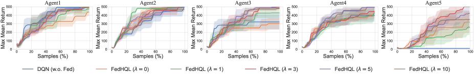
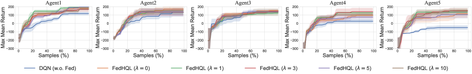
Figure 3: Individual learning curves of ($N=5$) agents running FedHQL with different inter-agent exploration coefficients (FedHQL ($\lambda\!=\!0,1,3,5,10$) against independent training (DQN (w.o. Fed)) on the CartPole (top) and LunarLander (bottom) environments.

Pertaining to the budget of each agent, we stipulate a fixed budget of maximum $2\times 10^{6}$ environment interactions for CartPole and $4\times 10^{6}$ environment interactions for LunarLander. The discount factor is set to be 0.999 for CartPole and 0.990 for LunarLander. The hyper-parameters of FedHQL are set as follows: we use number of gradient steps $\kappa$=64, maximum federation time horizon $H_{\text{Fed}}$=16, FedTD learning rate $\alpha_{\text{s}}$=0.05, and we set the batch size of the queries to be 128. The number of self-learning steps is set to be 5k for CartPole and 10k for LunarLander. And we update the target network of the backbone DQN algorithm every 1k steps for CartPole and 2k steps for LunarLander. Other experimental details follow the default settings of stable baselines (Raffin et al., 2021) and are kept the same for every set of experiments across different runs for a fair comparison. In all experiments, we report the metric max mean return, in which we compute the average/mean performance of every 10 test episodes during training and report the max value among them. Each experiment is repeated with 5 independent runs with 80% bootstrap confidence intervals using random seeds from 0 to 4.

5.2 Efficacy in Improving System Welfare

We firstly investigate the efficacy of FedHQL in improving the system welfare, i.e., the first objective of FedRL-HALE (Sec. 3.1). In particular, given the fixed budget of each agent, we examine the average performance of agents versus the average consumption of the budget per agent. The results in both tasks are plotted in Fig. 4. Of note, the sample cost incurred at the server is also included in the computation of the budget of an agent in FedHQL following (4). The figures show that FedHQL with different choices of inter-agent exploration coefficients, FedHQL ($\lambda=0,1,3,5,10$), significantly improves the average performance per agent over that of independent self-learning, DQN (w.o. Fed). For example, in the LunarLander task, an agent is expected to consume at least $40\%$ of its budget (i.e., total $1.6\text{m}=4\times 10^{6}\times 0.4$ interactions) on average to receive positive returns while an agent in FedHQL ($\lambda=1$) can achieve a performance close to 100 using only about $20\%$ of its budget (i.e., total $0.8\text{m}=4\times 10^{6}\times 0.2$ interactions). The results also suggest that FedHQL is less sensitive to the choice of $\lambda$ in the LunarLander task compared to the CartPole task, which we think is because any degree of inter-agent exploration (i.e., collaboration among agents) would help significantly in the more difficult task of LunarLander.

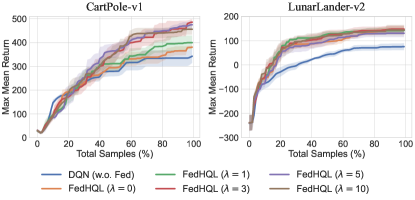
Figure 4: Learning curves of FedHQL ($N=5$ agents) with different inter-agent exploration coefficients (FedHQL ($\lambda\!=\!0,1,3,5,10$) against independent self-learning of agents (DQN (w.o. Fed)) on the CartPole (left) and LunarLander (right) tasks.

5.3 Effectiveness in Improving Individual Agents

Next, we verify the effectiveness of FedHQL in boosting the sample efficiency of each participating agent with high probability, i.e., the second objective of FedRL-HALE (Sec. 3.1). In this set of experiments, we report the performance versus the consumed samples of each individual agent (Agent1 to Agent5) during the corresponding training process. Fig. 3 shows the results for the CartPole (top) and LunarLander (bottom) tasks. The figures show that for both tasks, FedHQL is able to boost the sample efficiency for most agents. For example, Agent1 needs to consume over $60\%$ of its budget to reach a performance of 100 in LunarLander with independent self-learning, DQN (w.o. Fed). If Agent1 participates in FedHQL ($\lambda=1$) with the other four agents, its performance can be boosted to around 150 with just $20\%$ of its budget. Similar results can be observed from the other four agents on the LunarLander environment.

Interestingly, FedHQL ($\lambda=0$) renders the performance of Agent1 and Agent3 slightly worse than their corresponding independent self-learning (DQN (w.o. Fed)). This is because Agent5 (whose policy network is poorly parameterized) fails to learn the CartPole task within the given budget, causing inaccurate knowledge (estimation of the action values) of Agent5 to be sent to the server. As discussed in Sec. 4.2, FedUCB with $\lambda=0$ encourages the server to strongly exploit the group knowledge $\bar{Q}$ which is inaccurate due to the misleading knowledge contributed by Agent5. As a result, the performances of Agent1 and Agent3 in FedHQL ($\lambda=0$) deteriorate slightly while their performance is still improved with FedHQL ($\lambda=1,3,5,10$), which corroborates our theoretical insights on FedUCB (Sec. 4.2). Moreover, it is worth noting that FedHQL ($\lambda=0,1,3,5,10$) significantly improves the performance of Agent5 from being completely unlearnable to solving the task with nearly maximum return. Similar experimental results with more $N=10$ agents are given in Appendix B.

6 Conclusion

In this work, we introduce a practical formulation of FedRL with heterogeneous and black-box agents and discuss the unique challenges posed by this novel setting. We have presented principled solutions to these challenges and proposed the FedHQL algorithm. Due to the difficulty in analyzing the convergence of Q-learning and that heterogeneous agents may utilize arbitrarily non-linear policy parameterization, the convergence of FedHQL and its correlation with the number of agents are not studied in this work, which we consider promising future directions.

Appendix A Algorithm Pseudocode

Due to space constraints, the pseudocode for the proposed FedHQL algorithm is deferred here and depicted in Algorithm 1.a&1.b. The graphical illustration of FedHQL is also reproduced below (Fig. 5).

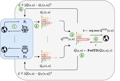
Figure 5: Graphical illustration of FedHQL.

Of note, the above process can be implemented in asynchronous batches using the reliable broadcast protocol from distributed computing (Chang & Maxemchuk, 1984).

Algorithm 1.a FedHQL (central server)

0:  query state $s_{0}$, inter-agent exploration constant $\lambda$, maximum federation time horizon $H_{\text{fed}}$, FedTD learning rate $\alpha_{\text{s}}$

1:  while a total budget of interactions is not exhausted do

2:     // Begin self-learning process

3:     Let each agent perform self-learning

4:     // Begin federation process

5:     $t\leftarrow 0$

6:     while $s_{t}$ is not terminating And $t<H_{\text{fed}}$ do

7:        Broadcast $s_{t}$ to all agents; Receive $\{Q_{n}(s_{t},a),\forall a\}_{n=1}^{N}$

8:        Compute $\bar{Q}(s_{t},a),{Q}^{\text{std}}(s_{t},a),Q^{\text{UCB}}(s_{t},a),\forall a$ according to Eq. (10), (11), (12)

9:        $\bar{a}_{t}\leftarrow\arg\max_{a}Q^{\text{UCB}}(s_{t},a)$

10:        Sample $(s_{t},\bar{a}_{t},s_{t+1},r_{t})$ by executing $\bar{a}_{t}$

11:        Broadcast $s_{t+1}$ to all agents; Receive $\{Q_{n}(s_{t+1},\forall a)\}_{n=1}^{N}$

12:        Perform $\textbf{FedTD}(\bar{Q}(s_{t},\bar{a}_{t}),r_{t},\alpha_{\text{s}})$ according to Eq. (4.3)

13:        Broadcast $\bar{Q}(s_{t},\bar{a}_{t})$ to all agents; Wait for agents to perform individual improvement

14:        $t\leftarrow t+1$

Algorithm 1.b FedHQL (agent $n$)

0:  arbitrary network $Q_{n}$ parameterized by $\theta_{n}$, intra-agent exploration coefficient $\epsilon_{n}$, individual learning rate $\alpha_{n}$, number of gradient steps $\kappa$

1:  if Self-learning signal received from server then

2:     Perform self-learning: $Q_{n}\leftarrow$ Self-learning($Q_{n}$, $\epsilon_{n}$, $\alpha_{n}$)

3:  if $\bar{Q}(s_{t},\bar{a}_{t})$ received from server then

4:     Update $Q_{n}$ according to Eq. (15) & (16) for $\kappa$ steps

5:  if $s_{t}$ received from server then

6:     Answer query $Q_{n}$ at received $s_{t}$ and send it to central server

Appendix B Experiments with More Agents

We repeat the same sets of experiments with $N=10$ agents, whose configurations are depicted in Table 2, to further verify the efficacy of FedHQL in improving the system welfare and its effectiveness in improving the sample efficiency of individual participating agents.

Table 2: Configurations of $N=10$ agents

Agent	Network	Learning rates	Intra-exploration coefficient
1	64x64 (ReLU)	0.01	0.01
2	128x128 (ReLU)	0.1	0.1
3	32x32 (Tanh)	0.01	0.05
4	16x16 (ReLU)	0.01	0.01
5	8x8x8 (ReLU)	0.01	0.01
6	64x64 (Tanh)	0.02	0.01
7	128x128 (ReLU)	0.02	0.1
8	32x32 (ReLU)	0.02	0.05
9	16x16 (Tanh)	0.05	0.01
10	8x8x8 (Tanh)	0.05	0.01

B.1 Efficacy of FedHQL ($N=10$ agents) in Improving System Welfare

Similar conclusion from Sec. 5.2 and Sec. 5.3 can also be drawn from both the two tasks. For example, in the CartPole task, an agent needs to sample at least $20\%$ of its budget (i.e., total $0.4\text{m}=2\times 10^{6}\times 0.2$ interactions) on average to receive an average return of 300 while an agent in FedHQL ($\lambda=1,3$) can achieve a performance close to 400 within the same consumption of $20\%$ of its budget. Also in the LunarLander task, an agent is expected to consume at least $20\%$ of its budget (i.e., total $0.8\text{m}=4\times 10^{6}\times 0.2$ interactions) on average to receive positive returns while an agent in FedHQL ($\lambda=3$) can achieve a performance close to 100 within the same consumption of $20\%$ of its budget. These performance improvements over the $N=10$ heterogeneous and black-box agents further verify the empirical performance of FedHQL in improving the sample efficiency of RL agents from the system perspective.

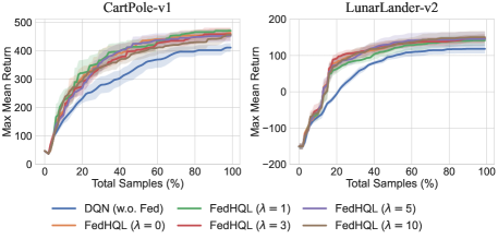
Figure 6: Learning curves of FedHQL ($N=10$ agents) with different inter-agent exploration coefficients (FedHQL ($\lambda\!=\!0,1,3,5,10$) against independent self-learning of agents (DQN (w.o. Fed)) on the CartPole (left) and LunarLander (right) environments.

B.2 Effectiveness of FedHQL ($N=10$ agents) in Improving Individual Agents

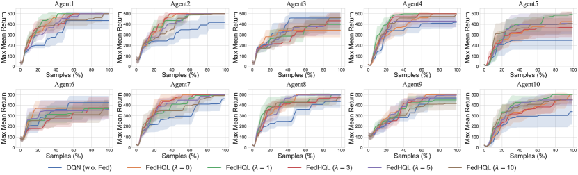
Figure 7: Individual learning curves of each agent running FedHQL ($N=10$ agents) with different inter-agent exploration coefficients (FedHQL ($\lambda\!=\!0,1,3,5,10$) against independent training (DQN (w.o. Fed)) on the CartPole environment.

Fig. 7 and Fig. 8 show the results used to verify the effectiveness of FedHQL in boosting the sample efficiency of each participating agent with high probability, i.e., the second objective of FedRL-HALE (Sec. 3.1), for CartPole and LunarLander, respectively. Interestingly, FedHQL ($\lambda=0$) renders the performance of Agent3 slightly worse than their corresponding independent self-learning (DQN (w.o. Fed)). This is because Agent5 and Agent 10 (whose policy networks are poorly parameterized) fail to learn the CartPole task within the given budget, causing inaccurate knowledge (estimation of the action values) of Agent5 and Agent 10 to be sent to the server. As discussed in Sec. 4.2, FedUCB with $\lambda=0$ encourages the server to strongly exploit the group knowledge $\bar{Q}$ which is inaccurate due to the misleading knowledge contributed by Agent5 and Agent 10. As a result, the performances of Agent3 in FedHQL ($\lambda=0$) deteriorate slightly in the early training stage. Moreover, it is worth noting that FedHQL ($\lambda=0,1,3,5,10$) significantly improves the performance of Agent5 and Agent10 from being completely unlearnable to solving the task with nearly maximum return, which further verifies the effectiveness of FedHQL in improving individual agents with high probability.

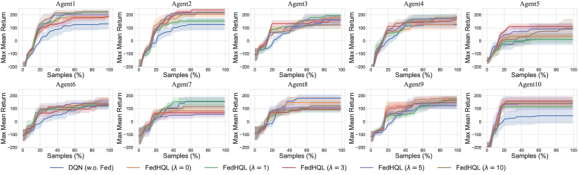
Figure 8: Individual learning curves of each agent running FedHQL ($N=10$ agents) with different inter-agent exploration coefficients (FedHQL ($\lambda\!=\!0,1,3,5,10$) against independent training (DQN (w.o. Fed)) on the LunarLander environment.

References

- Audibert et al. (2009) Audibert, J.-Y., Munos, R., and Szepesvári, C. Exploration–exploitation tradeoff using variance estimates in multi-armed bandits. Theoretical Computer Science, 410(19):1876–1902, 2009.
- Bajaj et al. (2021) Bajaj, I., Arora, A., and Hasan, M. F. Black-box optimization: Methods and applications. In Black Box Optimization, Machine Learning, and No-Free Lunch Theorems, pp. 35–65. Springer, 2021.
- Brockman et al. (2016) Brockman, G., Cheung, V., Pettersson, L., Schneider, J., Schulman, J., Tang, J., and Zaremba, W. Openai gym. arXiv:1606.01540, 2016.
- Cesa-Bianchi et al. (2017) Cesa-Bianchi, N., Gentile, C., Lugosi, G., and Neu, G. Boltzmann exploration done right. In Advances in neural information processing systems, volume 30, 2017.
- Chang & Maxemchuk (1984) Chang, J.-M. and Maxemchuk, N. F. Reliable broadcast protocols. ACM Transactions on Computer Systems (TOCS), 2(3):251–273, 1984.
- Chen et al. (2021) Chen, L., Lu, K., Rajeswaran, A., Lee, K., Grover, A., Laskin, M., Abbeel, P., Srinivas, A., and Mordatch, I. Decision transformer: Reinforcement learning via sequence modeling. Advances in neural information processing systems, 34:15084–15097, 2021.
- Chen et al. (2022) Chen, Y., Zhang, X., Zhang, K., Wang, M., and Zhu, X. Byzantine-robust online and offline distributed reinforcement learning. arXiv preprint arXiv:2206.00165, 2022.
- Espeholt et al. (2018) Espeholt, L., Soyer, H., Munos, R., Simonyan, K., Mnih, V., Ward, T., Doron, Y., Firoiu, V., Harley, T., Dunning, I., et al. Impala: Scalable distributed deep-rl with importance weighted actor-learner architectures. In International Conference on Machine Learning, pp. 1407–1416. PMLR, 2018.
- Fan et al. (2021) Fan, F. X., Ma, Y., Dai, Z., Jing, W., Tan, C., and Low, B. K. H. Fault-tolerant federated reinforcement learning with theoretical guarantee. In Advances in Neural Information Processing Systems, 2021.
- Fujita et al. (2022) Fujita, K., Fujimura, S., Sun, Y., Esaki, H., and Ochiai, H. Federated reinforcement learning for the building facilities. In 2022 IEEE International Conference on Omni-layer Intelligent Systems (COINS), pp. 1–6, 2022. doi: 10.1109/COINS54846.2022.9854959.
- Horgan et al. (2018) Horgan, D., Quan, J., Budden, D., Barth-Maron, G., Hessel, M., Van Hasselt, H., and Silver, D. Distributed prioritized experience replay. arXiv preprint arXiv:1803.00933, 2018.
- Jin et al. (2022) Jin, H., Peng, Y., Yang, W., Wang, S., and Zhang, Z. Federated reinforcement learning with environment heterogeneity. In International Conference on Artificial Intelligence and Statistics, pp. 18–37. PMLR, 2022.
- Johnson & Zhang (2013) Johnson, R. and Zhang, T. Accelerating stochastic gradient descent using predictive variance reduction. In Advances in neural information processing systems, pp. 315–323, 2013.
- Kairouz et al. (2021) Kairouz, P., McMahan, H. B., Avent, B., Bellet, A., Bennis, M., Bhagoji, A. N., Bonawitz, K., Charles, Z., Cormode, G., Cummings, R., et al. Advances and open problems in federated learning. Foundations and Trends® in Machine Learning, 14(1–2):1–210, 2021.
- Khodadadian et al. (2022) Khodadadian, S., Sharma, P., Joshi, G., and Maguluri, S. T. Federated reinforcement learning: Linear speedup under markovian sampling. In International Conference on Machine Learning, pp. 10997–11057. PMLR, 2022.
- Konečnỳ et al. (2016) Konečnỳ, J., McMahan, H. B., Ramage, D., and Richtárik, P. Federated optimization: Distributed machine learning for on-device intelligence. arXiv preprint arXiv:1610.02527, 2016.
- Lattimore & Szepesvári (2020) Lattimore, T. and Szepesvári, C. Bandit algorithms. Cambridge University Press, 2020.
- Liang et al. (2023) Liang, X., Liu, Y., Chen, T., Liu, M., and Yang, Q. Federated transfer reinforcement learning for autonomous driving. In Federated and Transfer Learning, pp. 357–371. Springer, 2023.
- Liu et al. (2019) Liu, B., Wang, L., and Liu, M. Lifelong federated reinforcement learning: A learning architecture for navigation in cloud robotic systems. IEEE Robotics and Automation Letters, 4(4):4555–4562, 2019. doi: 10.1109/LRA.2019.2931179.
- McMahan et al. (2017) McMahan, B., Moore, E., Ramage, D., Hampson, S., and y Arcas, B. A. Communication-efficient learning of deep networks from decentralized data. In Artificial intelligence and statistics, pp. 1273–1282. PMLR, 2017.
- Mnih et al. (2013) Mnih, V., Kavukcuoglu, K., Silver, D., Graves, A., Antonoglou, I., Wierstra, D., and Riedmiller, M. Playing atari with deep reinforcement learning. arXiv:1312.5602, 2013.
- Mnih et al. (2016) Mnih, V., Badia, A. P., Mirza, M., Graves, A., Lillicrap, T., Harley, T., Silver, D., and Kavukcuoglu, K. Asynchronous methods for deep reinforcement learning. In International conference on machine learning, pp. 1928–1937. PMLR, 2016.
- Nadiger et al. (2019) Nadiger, C., Kumar, A., and Abdelhak, S. Federated reinforcement learning for fast personalization. In 2019 IEEE Second International Conference on Artificial Intelligence and Knowledge Engineering (AIKE), pp. 123–127, 2019. doi: 10.1109/AIKE.2019.00031.
- Nair et al. (2015) Nair, A., Srinivasan, P., Blackwell, S., Alcicek, C., Fearon, R., De Maria, A., Panneershelvam, V., Suleyman, M., Beattie, C., Petersen, S., et al. Massively parallel methods for deep reinforcement learning. arXiv preprint arXiv:1507.04296, 2015.
- Papini et al. (2018) Papini, M., Binaghi, D., Canonaco, G., Pirotta, M., and Restelli, M. Stochastic variance-reduced policy gradient. In International conference on machine learning, pp. 4026–4035. PMLR, 2018.
- Raffin et al. (2021) Raffin, A., Hill, A., Gleave, A., Kanervisto, A., Ernestus, M., and Dormann, N. Stable-baselines3: Reliable reinforcement learning implementations. Journal of Machine Learning Research, 2021.
- Rieke et al. (2020) Rieke, N., Hancox, J., Li, W., Milletari, F., Roth, H. R., Albarqouni, S., Bakas, S., Galtier, M. N., Landman, B. A., Maier-Hein, K., et al. The future of digital health with federated learning. NPJ digital medicine, 3(1):1–7, 2020.
- Sutton & Barto (2018) Sutton, R. S. and Barto, A. G. Reinforcement learning: An introduction. MIT press, 2018.
- Wang et al. (2020) Wang, X., Wang, C., Li, X., Leung, V. C., and Taleb, T. Federated deep reinforcement learning for internet of things with decentralized cooperative edge caching. IEEE Internet of Things Journal, 7(10):9441–9455, 2020.
- Watkins (1989) Watkins, C. J. C. H. Learning from delayed rewards. PhD thesis, University of Cambridge England, 1989.
- Xue et al. (2021) Xue, Z., Zhou, P., Xu, Z., Wang, X., Xie, Y., Ding, X., and Wen, S. A resource-constrained and privacy-preserving edge-computing-enabled clinical decision system: A federated reinforcement learning approach. IEEE Internet of Things Journal, 8(11):9122–9138, 2021.
- Yahya et al. (2017) Yahya, A., Li, A., Kalakrishnan, M., Chebotar, Y., and Levine, S. Collective robot reinforcement learning with distributed asynchronous guided policy search. In 2017 IEEE/RSJ International Conference on Intelligent Robots and Systems (IROS), pp. 79–86. IEEE, 2017.
- Yu et al. (2020) Yu, S., Chen, X., Zhou, Z., Gong, X., and Wu, D. When deep reinforcement learning meets federated learning: Intelligent multitimescale resource management for multiaccess edge computing in 5g ultradense network. IEEE Internet of Things Journal, 8(4):2238–2251, 2020.
- Zhuo et al. (2019) Zhuo, H. H., Feng, W., Lin, Y., Xu, Q., and Yang, Q. Federated deep reinforcement learning. arXiv:1901.08277, 2019.