Conformal Prediction for Trustworthy Detection of Railway Signals

Abstract

We present an application of conformal prediction, a form of uncertainty quantification with guarantees, to the detection of railway signals. State-of-the-art architectures are tested and the most promising one undergoes the process of conformalization, where a correction is applied to the predicted bounding boxes (i.e. to their height and width) such that they comply with a predefined probability of success. We work with a novel exploratory dataset of images taken from the perspective of a train operator, as a first step to build and validate future trustworthy machine learning models for the detection of railway signals.

Introduction

In this paper we focus on building a trustworthy detector of railway light signals via Machine Learning (ML) . We apply Uncertainty Quantification (UQ) to the problem of Object Detection (OD) (Zhao et al. 2019) via the distribution-free, non-asymptotic and model-agnostic framework of Conformal Prediction (CP). CP is computationally lightweight, can be applied to any (black-box) predictor with minimal hypotheses and efforts, and has rigorous statistical guarantees.

We give a brief overview of UQ for OD and the CP method we apply to our use case. After selecting a pre-trained model among the state-of-the-art architectures, we give some insights on how UQ techniques can quantify the trustworthiness of OD models, which could be part of a critical Artificial Intelligence (AI) system, and their potential role in certifying such technologies for future industrial deployment.

The Industrial Problem

AI can work as a complementary tool to enhance existing technologies, like in the automotive industry (Alecu et al. 2022). We can draw a parallel with the railway sector. While main lines (e.g. high-speed lines) already have in-cabin signaling and can be automatized (Singh et al. 2021), this is too costly to apply to the whole network. Consequently, on secondary lines, drivers can be subject to a larger cognitive load, and therefore strain, from signals and the environment. Assisting drivers with AI-based signaling recognition could facilitate the operations.

With respect to Figure 1, our application corresponds to point (1) of their process based on multiple ML tasks: trustworthiness concerns can grow with the number of ML components. For a recent overview on the technical and regulatory challenges raised by the safety of ML systems in the railway and automotive industries, see Alecu et al. (2022).

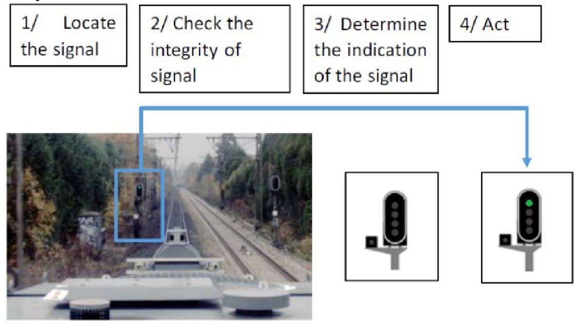
Figure 1: Example of pipeline where an AI system acts following ML-based predictions. Source: Alecu et al. (2022).

Building an exploratory dataset

Currently, there is no standard benchmark for railway signaling detection. Stemming from the dataset FRSign of Harb et al. (2020) and their insights, our own iterations made us aware of some additional needs. Notably, our new dataset aims for images to be independent and identically distributed (i.i.d), and therefore, raw sequences cannot be considered. Moreover, our new dataset features increased variability (more railway lines, environmental and weather conditions, etc.) which could enable more accurate predictions in real-world scenarios. Finally, we generalize the task from single to multi-object detection, laying the foundations for future work in instance segmentation.

We would expect a deployable system to work whenever a human operator is successful: at night, with rain, or even when the signals are partially occluded by foliage. Within our exploratory dataset, we included different light conditions but this is far from exhaustive; these issues will be taken into account in future iterations of the dataset.

Characteristics	Quantity
Railway lines	25
Images per line (average)	55.8 $\pm$ 29.7
Images in dataset	1395
Dimensions (pixels)	1280 $\times$ 720
Bounding boxes (total)	2382

Table 1: Characteristics of our dataset

As source data, we used some video footage taken on French railway lines, with the approval of the creators. To extract the samples, we acted as follows. On 25 videos of average duration about 1.5 hour, we extract on average 55 images per video by running a pretrained object detector with a low objectness threshold, and we keep a minimum interval of 3 seconds between detections, to prevent excessive dependence between images. We kept the images without the associated detections. We then manually annotated all visible railway signals. In Table 1 we report the statistics of our dataset.

Related Works

Among the OD architecture, we point out YOLO (Redmon et al. 2016) and its variants: they propose a one-stage detection combining convolution layers with regression and classification tasks. Howard et al. (2017), with MobileNets, introduced the concept of depth-wise separable convolutions to reduce the number of parameters and accelerate the inference. As for the recent introduction of transformer layers, we find DETR (Carion et al. 2020) and ViT (Dosovitskiy et al. 2020), among others. These networks reach state-of-the-art performances, and seem well-suited to transfer learning. Finally, DiffusionDet Chen et al. (2022) recently formulated OD as a denoising diffusion problem, from random noisy boxes to real objects, with state-of-the-art performance.

Uncertainty Quantification in Object Detection

UQ is an important trigger to deploy OD in transport systems. We find probabilistic OD (Hall et al. 2020), where the probability distributions of the bounding boxes and classes are predicted; Bayesian models like in Harakeh, Smart, and Waslander (2020) and Bayesian approximations (Deepshikha et al. 2021) are also found in the literature. We point out the distribution-free approach of Li et al. (2022): they build probably approximately correct prediction sets via concentration inequalities, estimated via a held-out calibration set. They control the coordinates of the boxes but also the proposal and objectness scores, resulting in more and larger boxes. Finally, de Grancey et al. (2022) proposed an extension of CP to OD, which will be the framework of choice in our exploratory study.

Conformalizing Object Detection

Conformal Prediction (CP) (Vovk, Gammerman, and Shafer 2022; Angelopoulos and Bates 2021) is a family of methods to perform UQ with guarantees under the sole hypothesis of data being independent and identically distributed (or more generally exchangeable). For a specified (small) error rate $\alpha\in(0,1)$, at inference, the CP procedure will yield prediction sets $C_{\alpha}(X)$ that contain the true target values $Y$ with probability:

$$\mathbb{P}\big{(}Y_{new}\in C_{\alpha}(X_{new})\big{)}\geq 1-\alpha.$$ (1)

This guarantee holds true, on average, over all images at inference and over many repetitions of the CP procedure. However, it is valid for any distribution of the data $\mathbb{P}_{XY}$, any sample size and any predictive model $\widehat{f}$, even if it is misspecified or a black box. The probability $1-\alpha$ is the nominal coverage and the empirical coverage on $n_{\text{test}}$ points is $\sum_{i=1}^{n_{\text{test}}}\mathbb{I}\{Y_{i}\in{C}_{\alpha}(X_{i})\}/n_{\text{test}}$.

We focus on split CP (Papadopoulos et al. 2002; Lei et al. 2018), where one needs a set of calibration data $D_{cal}$ drawn from the same $\mathbb{P}_{XY}$ as the test data, with no need to access the training data. At conformalization, we compute the nonconformity scores, to quantify the uncertainty on held-out data. At inference, CP adds a margin around the bounding box predicted by a pretrained detector $\widehat{f}$.

Split conformal object detection

We follow de Grancey et al. (2022). Let $k=1,\dots,n_{box}$ index every ground-truth box in $D_{cal}$ that was detected by $\widehat{f}$, disregarding their source image. Let $Y^{k}=(x_{\text{min}}^{k},y_{\text{min}}^{k},x_{\text{max}}^{k},y_{\text{max}}^{k})$ be the coordinates of the $k$-th box and $\widehat{Y}^{k}=(\hat{x}_{\text{min}}^{k},\hat{y}_{\text{min}}^{k},\hat{x}_{\text{max}}^{k},\hat{y}_{\text{max}}^{k})$ its prediction.

In de Grancey et al. (2022) their nonconformity score, which we refer to as additive, is defined as:

$$R_{k}=(\hat{x}_{\text{min}}^{k}-{x}_{\text{min}}^{k},\hat{y}_{\text{min}}^{k}-{y}_{\text{min}}^{k},{x}_{\text{max}}^{k}-\hat{x}_{\text{max}}^{k},{y}_{\text{max}}^{k}-\hat{y}_{\text{max}}^{k}).$$ (2)

We further define the multiplicative one as:

$$R_{k}=\big{(}\frac{\hat{x}_{\text{min}}^{k}-{x}_{\text{min}}^{k}}{\widehat{w}^{k}},\frac{\hat{y}_{\text{min}}^{k}-{y}_{\text{min}}^{k}}{\widehat{h}^{k}},\frac{{x}_{\text{max}}^{k}-\hat{x}_{\text{max}}^{k}}{\widehat{w}^{k}},\frac{{y}_{\text{max}}^{k}-\hat{y}_{\text{max}}^{k}}{\widehat{h}^{k}}\big{)}$$ (3)

where the prediction errors are scaled by the predicted width $\widehat{w}^{k}$ and height $\widehat{h}^{k}$. This is similar to Papadopoulos et al. (2002), and a natural extension to de Grancey et al. (2022).

Split conformal object detection goes as follows:

• choose a nonconformity score: e.g. Equation (2) or (3);

• Run a pairing mechanism, to associate predicted boxes with true boxes (see following paragraphs);

• For every coordinate $c\in\{x_{\text{min}},y_{\text{min}},x_{\text{max}},y_{\text{max}}\}$, let $\bar{R}^{c}=\left(R_{k}^{c}\right)_{k=1}^{n_{box}}$;

• compute $q_{1-\frac{\alpha}{4}}^{c}=\lceil(n_{box}+1)(1-\frac{\alpha}{4})\rceil$-th element of the sorted sequence $\bar{R}^{c}$, $\forall c\in\{x_{\text{min}},y_{\text{min}},x_{\text{max}},y_{\text{max}}\}$.

Since we work with four coordinates, for statistical reasons, we adjust the quantile order from $(1-\alpha)$ to $(1-\frac{\alpha}{4})$ using the Bonferroni correction. We conformalize box-wise: we want to be confident that when we detect correctly an object (“true positive”), we capture the entire ground-truth box with a frequency of at least $(1-\alpha)$, on average. During calibration (point 2. above), for all the true positive predicted boxes ($\widehat{Y}^{TP}_{cal}$), we compute the nonconformity score between the true box and the prediction. The pairing mechanism is the same as the NMS used in OD, that is, for each ground-truth bounding box, the predicted bounding boxes (not already assigned to a ground truth) are tested in decreasing order of their confidence scores. The first predicted box with an IoU above a set threshold is assigned to the ground truth box. Note that while building ($\widehat{Y}^{TP}_{cal}$), we do not consider false negatives (due to $\widehat{f}$) which cannot be taken care of by box-wise CP.

At inference, the additive split conformal object detection prediction box is built as:

$$\widehat{C}_{\alpha}(X)=\{\widehat{x}_{\text{min}} -q_{1-\frac{\alpha}{4}}^{x_{\text{min}}},\,\widehat{y}_{\text{min}}-q_{1-\frac{\alpha}{4}}^{y_{\text{min}}},$$ (4)

$$\widehat{x}_{\text{max}} +q_{1-\frac{\alpha}{4}}^{x_{\text{max}}},\,\widehat{y}_{\text{max}}+q_{1-\frac{\alpha}{4}}^{y_{\text{max}}}\}.$$

The multiplicative conformal prediction box is:

$$\widehat{C}_{\alpha}(X)=\{\widehat{x}_{\text{min}} -\widehat{w}\cdot q_{1-\frac{\alpha}{4}}^{x_{\text{min}}},\,\widehat{y}_{\text{min}}-\widehat{h}\cdot q_{1-\frac{\alpha}{4}}^{y_{\text{min}}},$$ (5)

$$\widehat{x}_{\text{max}} +\widehat{w}\cdot q_{1-\frac{\alpha}{4}}^{x_{\text{max}}},\,\widehat{y}_{\text{max}}+\widehat{h}\cdot q_{1-\frac{\alpha}{4}}^{y_{\text{max}}}\}.$$

Experiments

We split our dataset into three subsets: validation, calibration and test (respectively of size 300, 700, 395). We compare, using the validation set, the performance of YOLOv5, DETR and DiffusionDet, pretrained on COCO (Lin et al. 2014), as candidate base predictors $\widehat{f}$, restricting the detection to the class “traffic light”. Commonly, OD models are evaluated using the Average Precision (AP), which is the Area Under the recall-precision Curve. AP incorporates the precision-recall trade-off, and the best value is reached when precision and recall are maximized for all objectness thresholds. In our application (Table 2), the AP for YOLOv5 is low, while DETR gives better results, and DiffusionDet is significantly superior to the others. We therefore use the DiffusionDet model for our conformalization. However, AP metrics alone do not give a complete picture to select OD architecture.

	Average Precision
	IoU $\geq 0.3$	IoU $\geq 0.8$
YOLOv5s†	0.239	0.033
YOLOv5x†	0.287	0.093
DETR resnet50	0.531	0.008
DiffusionDet	0.839	0.325

Table 2: Comparing models via AP for two IoU threshold levels. ^†: v5s and v5x respectively correspond to a small and a large configurations of YOLOv5.

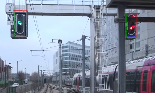
Figure 2: Bounding boxes as predicted by the ML predictor (blue), their conformalized version with additive scores (green) and the ground truth (red). Example of images used in conformalization and testing, cropped for readability.

Detector evaluation with box-wise conformalization

We evaluate OD performances (Table 3) by box-wise conformal prediction, reporting the estimated quantiles $q_{1-\frac{\alpha}{4}}^{c}$ at the desired risk level. A higher quantile reveals a higher uncertainty of OD predictions.In order to compare additive and multiplicative quantiles which are qualitatively different, we report the stretch: the ratio of the areas of the conformalized and predicted boxes. We display examples of additive and multiplicative conformalized boxes respectively on Figure 2 and Figure 3.

	$q_{1-\alpha}^{x_{\text{min}}}$	$q_{1-\alpha}^{y_{\text{min}}}$	$q_{1-\alpha}^{x_{\text{max}}}$	$q_{1-\alpha}^{y_{\text{max}}}$	Stretch∗
Additive †	4.74	7.16	6.91	5.67	$\times$ 2.857
Multiplicative ‡	0.22	0.37	0.21	0.21	$\times$ 2.259

Table 3: Conformalization margins on DiffusionDet. ^∗: average increase in the area of the boxes after conformalization. ^†: pixels; ^‡: fraction of $\widehat{w}$ or $\widehat{h}$.

Results

Empirically, CP works as expected: in Table 4, we see that conformalized coverage is close to the nominal level of $(1-\alpha)=0.9$. Remark that the guarantee holds on average over multiple repetitions, hence we cannot expect to attain the requested nominal coverage with just one dataset.

CP method	None	Additive	Multiplicative
Empirical coverage	0.106	0.921	0.894

Table 4: Empirical coverage before and after conformalization, nominal coverage: $1-\alpha=0.90$. This replies to: “how many true boxes, when detected, were entirely covered by the predicted box?”

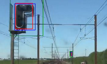
Figure 3: Bounding boxes as predicted by the ML predictor (blue), their conformalized version with multiplicative scores (green) and the ground truth (red). Example of images used in conformalization and testing, cropped for readability.

Interpretation of conformal bounding boxes

A conformalized predictor is only as good as its base predictor $\widehat{f}$. If the latter misses many ground truth boxes, guaranteeing $(1-\alpha)\,100\%$ correct predictions of a few boxes will still be a small number. That is, conformalization is not a substitute for careful training and fine-tuning of a detection architecture, but a complementary tool for certification.

The interest of capturing the whole box can be operational: our ML pipeline could rely on a conservative estimation of the ground-truth to carry out a control operations (e.g. running a ML subcomponent on the detection area).

Conclusion & perspectives

Given the insights from this exploratory study, we plan on building and publishing an augmented version of the dataset. The objective is to have a dedicated, high-quality benchmark for the scientific community and the transport industry. As mentioned above, CP works with exchangeable data. In the long term, if trustworthy AI components are to be deployed, the UQ guarantees will need to be adapted to streams of data: this will pose a theoretical challenge and one in the construction and validation of the dataset.

So far, the underlying criterion for successful prediction has been whether the ground truth box is entirely covered by the predicted box. This is strict, as having a system that guarantees to cover a big part of the truth, seems to be equally useful in practice. Bates et al. (2021), with their risk controlling prediction sets, and Angelopoulos et al. (2022), with conformal risk control, go in this direction. They extend the guarantee of CP to arbitrary losses, that can incorporate other operational needs.

References

- Alecu et al. (2022) Alecu, L.; Bonnin, H.; Fel, T.; Gardes, L.; Gerchinovitz, S.; Ponsolle, L.; Mamalet, F.; Jenn, É.; Mussot, V.; Cappi, C.; Delmas, K.; and Lefevre, B. 2022. Can we reconcile safety objectives with machine learning performances? In ERTS.
- Angelopoulos and Bates (2021) Angelopoulos, A. N.; and Bates, S. 2021. A Gentle Introduction to Conformal Prediction and Distribution-Free Uncertainty Quantification. arXiv:2107.07511.
- Angelopoulos et al. (2022) Angelopoulos, A. N.; Bates, S.; Fisch, A.; Lei, L.; and Schuster, T. 2022. Conformal Risk Control. arXiv:2208.02814.
- Bates et al. (2021) Bates, S.; Angelopoulos, A.; Lei, L.; Malik, J.; and Jordan, M. 2021. Distribution-Free, Risk-Controlling Prediction Sets. J. ACM, 68(6).
- Carion et al. (2020) Carion, N.; Massa, F.; Synnaeve, G.; Usunier, N.; Kirillov, A.; and Zagoruyko, S. 2020. End-to-end object detection with transformers. In ECCV 2020, 213–229. Springer.
- Chen et al. (2022) Chen, S.; Sun, P.; Song, Y.; and Luo, P. 2022. Diffusiondet: Diffusion model for object detection. arXiv:2211.09788.
- de Grancey et al. (2022) de Grancey, F.; Adam, J.-L.; Alecu, L.; Gerchinovitz, S.; Mamalet, F.; and Vigouroux, D. 2022. Object Detection with Probabilistic Guarantees: A Conformal Prediction Approach. In SAFECOMP 2022 Workshops. Springer.
- Deepshikha et al. (2021) Deepshikha, K.; Yelleni, S. H.; Srijith, P.; and Mohan, C. K. 2021. Monte carlo dropblock for modelling uncertainty in object detection. arXiv:2108.03614.
- Dosovitskiy et al. (2020) Dosovitskiy, A.; Beyer, L.; Kolesnikov, A.; Weissenborn, D.; Zhai, X.; Unterthiner, T.; Dehghani, M.; Minderer, M.; Heigold, G.; Gelly, S.; et al. 2020. An image is worth 16x16 words: Transformers for image recognition at scale. arXiv:2010.11929.
- Hall et al. (2020) Hall, D.; Dayoub, F.; Skinner, J.; Zhang, H.; Miller, D.; Corke, P.; Carneiro, G.; Angelova, A.; and Sünderhauf, N. 2020. Probabilistic object detection: Definition and evaluation. In Proceedings of WACV, 1031–1040.
- Harakeh, Smart, and Waslander (2020) Harakeh, A.; Smart, M.; and Waslander, S. L. 2020. Bayesod: A bayesian approach for uncertainty estimation in deep object detectors. In Proceedings of ICRA.
- Harb et al. (2020) Harb, J.; Rébéna, N.; Chosidow, R.; Roblin, G.; Potarusov, R.; and Hajri, H. 2020. FRSign: A Large-Scale Traffic Light Dataset for Autonomous Trains. arXiv:2002.05665.
- Howard et al. (2017) Howard, A. G.; Zhu, M.; Chen, B.; Kalenichenko, D.; Wang, W.; Weyand, T.; Andreetto, M.; and Adam, H. 2017. Mobilenets: Efficient convolutional neural networks for mobile vision applications. arXiv:1704.04861.
- Lei et al. (2018) Lei, J.; G’Sell, M.; Rinaldo, A.; Tibshirani, R. J.; and Wasserman, L. 2018. Distribution-Free Predictive Inference for Regression. Journal of the American Statistical Assoc.
- Li et al. (2022) Li, S.; Park, S.; Ji, X.; Lee, I.; and Bastani, O. 2022. Towards PAC Multi-Object Detection and Tracking. arXiv:2204.07482.
- Lin et al. (2014) Lin, T.-Y.; Maire, M.; Belongie, S.; Hays, J.; Perona, P.; Ramanan, D.; Dollár, P.; and Zitnick, C. L. 2014. Microsoft coco: Common objects in context. In ECCV. Springer.
- Papadopoulos et al. (2002) Papadopoulos, H.; Proedrou, K.; Vovk, V.; and Gammerman, A. 2002. Inductive confidence machines for regression. In Proceedings of ECML, 345–356. Springer.
- Redmon et al. (2016) Redmon, J.; Divvala, S.; Girshick, R.; and Farhadi, A. 2016. You only look once: Unified, real-time object detection. In Proceedings of CVPR, 779–788.
- Singh et al. (2021) Singh, P.; Dulebenets, M. A.; Pasha, J.; Gonzalez, E. D. R. S.; Lau, Y.-Y.; and Kampmann, R. 2021. Deployment of Autonomous Trains in Rail Transportation: Current Trends and Existing Challenges. IEEE Access, 9: 91427–91461.
- Vovk, Gammerman, and Shafer (2022) Vovk, V.; Gammerman, A.; and Shafer, G. 2022. Algorithmic Learning in a Random World. Springer, 2nd edition.
- Zhao et al. (2019) Zhao, Z.-Q.; Zheng, P.; Xu, S.-T.; and Wu, X. 2019. Object Detection With Deep Learning: A Review. IEEE Transactions on Neural Networks and Learning Systems, 30(11).