SNR/CRB-Constrained Joint Beamforming and Reflection Designs for RIS-ISAC Systems

Abstract

In this paper, we investigate the integration of integrated sensing and communication (ISAC) and reconfigurable intelligent surfaces (RIS) for providing wide-coverage and ultra-reliable communication and high-accuracy sensing functions. In particular, we consider an RIS-assisted ISAC system in which a multi-antenna base station (BS) simultaneously performs multi-user multi-input single-output (MU-MISO) communications and radar sensing with the assistance of an RIS. We focus on both target detection and parameter estimation performance in terms of the signal-to-noise ratio (SNR) and Cramér-Rao bound (CRB), respectively. Two optimization problems are formulated for maximizing the achievable sum-rate of the multi-user communications under an SNR constraint for target detection or a CRB constraint for parameter estimation, the transmit power budget, and the unit-modulus constraint of the RIS reflection coefficients. Efficient algorithms are developed to solve these two complicated non-convex problems. Extensive simulation results demonstrate the advantages of the proposed joint beamforming and reflection designs compared with other schemes. In addition, it is shown that more RIS reflection elements bring larger performance gains for direct-of-arrival (DoA) estimation than for target detection.

I Introduction

While wireless communication and radar sensing have been separately developed for decades, integrated sensing and communication (ISAC) is recently arising as a promising technology. The integration of communication and sensing systems has evolved from coexistence, cooperation, to co-design, thanks to similar hardware platforms and signal processing algorithms and the same evolution direction towards high-frequency wideband multi-antenna systems. ISAC not only allows communication and radar systems to share spectrum resources, but also enables a fully-shared platform transmitting unified waveforms to simultaneously perform communication and radar sensing functions, which significantly improves the spectral/energy/hardware efficiency [2]-[5]. It is foreseeable that in next-generation wireless networks, ISAC will be a supporting technology for diverse applications that require both high-quality ubiquitous wireless communications and high-accuracy sensing, e.g., smart home/factory, vehicular networks, etc. Therefore, researchers from both academia and industry have explored various ISAC implementations [6].

Advanced signal processing techniques have been investigated for designing the dual-functional transmit waveforms. Moreover, multi-input multi-output (MIMO) architectures are also widely considered in ISAC systems. By exploiting the spatial degrees of freedom (DoFs) of MIMO architectures, the waveform diversity for radar sensing and the beamforming gains and spatial multiplexing for communications can be greatly improved [7]. Therefore, the transmit waveforms/beamforming design for ISAC systems is a key problem [8]. Extensive investigations have been conducted using various communication and radar sensing metrics [9]-[12]. In addition, since radar sensing functions rely on analyzing received signal echoes, the receive beamforming is also jointly optimized to improve radar sensing performance [12]. Although these approaches greatly enhance communication and radar sensing functions, performance deterioration is still inevitable when encountering harsh propagation conditions. In such complex electromagnetic environments, the use of recently emerged reconfigurable intelligent surface (RIS) technology [13]-[15] provides a potentially revolutionary solution.

RIS technology has been regarded as another key enabler for future wireless networks owing to its capability of efficiently and intelligently shaping the propagation environment. An RIS is generally a two-dimensional meta-surface consisting of many passive reflecting elements that can be independently adjusted. By controlling specific parameters of the electronic circuits associated with each element, electromagnetic characteristics of the incident signals can be tuned, e.g., amplitude, phase-shift, etc. Passive beamforming gains can be achieved by cooperatively and intelligently adjusting these reflecting elements [16], [17]. The deployment of RIS establishes non-line-of-sight (NLoS) links between transmitter and receivers, which expands coverage and introduces additional DoFs for improving system performance. Therefore, the use of RIS in various wireless networks has been extensively investigated.

Inspired by extensive applications of RIS to various wireless communication systems [14], researchers have begun exploring the deployment of RIS in radar sensing [18] and ISAC systems [19], [20]. Studies for different RIS deployment scenarios with different communication and radar sensing metrics have been carried out [21]-[28]. The initial works [21]-[23] assumed that the RIS only assists with communications since it is deployed near the users with negligible impact on the target echoes. To further exploit the benefits of RIS, especially in improving radar sensing performance, the authors in [24]-[26] assumed that the RIS is deployed where the direct links between the base station (BS) and the users/target are blocked. However, it is likely more common that both the direct and reflected links contribute to communication and radar sensing functions, as considered in [27] and [28]. In particular, the authors in [27] focused on the single-user scenario and used the signal-to-noise ratio (SNR) metric for both communication and target detection, while the authors in [28] studied the more common multi-user scenario in the presence of clutter and proposed to maximize the radar signal-to-interference-plus-noise ratio (SINR) under communication constraints. However, the non-linear spatial-temporal beamforming assumed in [28] require more complicated hardware architectures and more complex algorithms. Moreover, in addition to the target detection function, parameter estimation is also an important task in radar sensing and should be further explored.

Motivated by above discussion, in this paper we focus on a general RIS-assisted ISAC system and consider both target detection and parameter estimation functions for the sensing component. In particular, we consider an RIS-assisted ISAC system in which a multi-antenna BS delivers data to multiple single-antenna users and simultaneously senses one point-like target with the assistance of an RIS. Our goal is to jointly design the BS transmit/receive beamforming and RIS reflection coefficients to maximize the multi-user communication performance as well as guaranteeing the target detection or direct-of-arrival (DoA) estimation performance. The main contributions of this paper are summarized as follows.

• First, we model the signals received at the users and the BS receive array, and then derive performance metrics for communications and radar sensing. Specifically, the sum-rate metric is utilized to evaluate the multi-user communications performance. For target detection, we show that the radar output SNR is positively proportional to the detection probability with a fixed probability of false alarm and derive a worst-case radar SNR as the performance metric. For target DoA estimation in the considered general case, we derive the Cramér-Rao bound (CRB) for estimating the target DoAs with respect to the BS and the RIS, which to our knowledge has not been investigated previously in the literature.

• Next, we formulate two optimization problems that maximize the sum-rate for multi-user communications subject to a radar SNR constraint for target detection or a CRB constraint for DoA estimation, the transmit power budget, and the unit-modulus constraint of the RIS reflection coefficients. In order to efficiently solve these two complicated non-convex problems, we develop two algorithms based on fractional programming (FP), majorization-minimization (MM), alternative direction method of multipliers (ADMM), and some sophisticated transformations.

• Finally, we provide extensive simulation studies to verify the effectiveness of the proposed schemes and associated algorithms. It is shown that the proposed designs achieve notably higher sum-rates compared with other schemes. We also present the enhanced beampattern to visually demonstrate the dual communications and radar sensing functions of the considered RIS-assisted ISAC system.

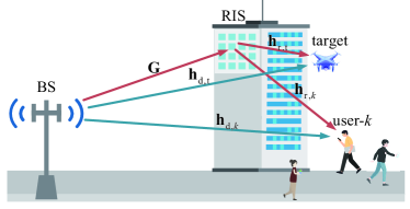
Figure 1: An RIS-assisted ISAC system.

II System and Signal Models

We consider an RIS-assisted ISAC system as shown in Fig. 1, where a colocated multi-antenna BS simultaneously performs multi-user communications and radar sensing with the assistance of an $N$-element RIS. In particular, the BS, which is equipped with $M_{\text{t}}$ transmit antennas and $M_{\text{r}}$ receive antennas arranged as uniform linear arrays (ULAs) with half-wavelength spacing, simultaneously serves $K$ single-antenna users and senses one target. For simplicity, in what follows we will assume $M_{\text{t}}=M_{\text{r}}=M$. In this work, we focus on two common and crucial radar sensing tasks: target detection, which aims to identify whether a target of interest is present, and parameter estimation, where the DoAs of the target signals with respect to the BS and the RIS are determined.

In order to simultaneously enable satisfactory communication and radar sensing functions, the dual-functional signal that is transmitted in the $l$-th time slot is given by [7]

$$\mathbf{x}[l]=\mathbf{W}_{\text{c}}\mathbf{s}_{\text{c}}[l]+\mathbf{W}_{\text{r}}\mathbf{s}_{\text{r}}[l]=\mathbf{W}\mathbf{s}[l],$$ (1)

where $\mathbf{s}_{\text{c}}[l]\in\mathbb{C}^{K}$ contains the communication symbols for the $K$ users with $\mathbb{E}\{\mathbf{s}_{\text{c}}[l]\mathbf{s}_{\text{c}}^{H}[l]\}=\mathbf{I}_{K}$, $\mathbf{s}_{\text{r}}[l]\in\mathbb{C}^{M}$ includes $M$ individual radar waveforms with $\mathbb{E}\{\mathbf{s}_{\text{r}}[l]\mathbf{s}_{\text{r}}^{H}[l]\}=\mathbf{I}_{M}$, $\mathbb{E}\{\mathbf{s}_{\text{c}}[l]\mathbf{s}_{\text{r}}^{H}[l]\}=\mathbf{0}$, and $\mathbf{W}_{\text{c}}\in\mathbb{C}^{M\times K}$ and $\mathbf{W}_{\text{r}}\in\mathbb{C}^{M\times M}$ denote the beamforming matrices for the communication symbols and radar waveforms, respectively. In addition, we define the combined beamforming matrix $\mathbf{W}\triangleq[\mathbf{W}_{\text{c}}~{}\mathbf{W}_{\text{r}}]$ and symbol vector $\mathbf{s}[l]\triangleq[\mathbf{s}_{\text{c}}^{T}[l]~{}\mathbf{s}_{\text{r}}^{T}[l]]^{T}$ for brevity. Then, the compound received signal at the $k$-th user can be expressed as

$$y_{k}[l]=(\mathbf{h}_{\text{d},k}^{T}+\mathbf{h}_{\text{r},k}^{T}\bm{\Phi}\mathbf{G})\mathbf{x}[l]+n_{k}[l],$$ (2)

where $\mathbf{h}_{\text{d},k}\in\mathbb{C}^{M}$, $\mathbf{h}_{\text{r},k}\in\mathbb{C}^{N}$, and $\mathbf{G}\in\mathbb{C}^{N\times M}$ denote the channels between the BS and the $k$-th user, between the RIS and the $k$-th user, and between the BS and the RIS, respectively. The channels $\mathbf{h}_{\text{d},k}$, $\mathbf{h}_{\text{r},k},~{}\forall k$, and $\mathbf{G}$ are assumed to follow Rician fading, e.g., the channel $\mathbf{G}$ is formulated as

$$\mathbf{G}=\alpha_{\text{G}}\sqrt{\frac{\kappa}{\kappa+1}}\mathbf{G}_{\text{LoS}}+\alpha_{\text{G}}\sqrt{\frac{1}{\kappa+1}}\mathbf{G}_{\text{NLoS}},$$ (3)

where $\alpha_{\text{G}}$ is the distance dependent pathloss, $\kappa$ represents the Rician factor, $\mathbf{G}_{\text{LoS}}$ is the LoS component that depends on the problem geometry, and $\mathbf{G}_{\text{NLoS}}$ denotes the NLoS Rayleigh fading components with zero mean and unit variance. In particular, $\mathbf{G}_{\text{LoS}}=\mathbf{a}_{N}^{T}(\theta_{\text{RB}})\mathbf{a}_{M}(\theta_{\text{BR}})$, where for a ULA the steering vector is given by $\mathbf{a}_{N}(\theta_{\text{RB}})\triangleq[1,e^{-\jmath\pi\sin\theta_{\text{RB}}},\ldots,e^{-\jmath(N-1)\pi\sin\theta_{\text{RB}}}]^{T}$, and $\theta_{\text{RB}}$ and $\theta_{\text{BR}}$ represent the DoA and direct-of-departure (DoD). We assume that the overall channel is known at the BS given advanced channel estimation approaches for RIS-aided communication systems. The RIS reflection matrix is defined as $\bm{\Phi}\triangleq\text{diag}\{\bm{\phi}\}$, where $\bm{\phi}\triangleq[\phi_{1},\ldots,\phi_{N}]^{T}$ is the vector of reflection coefficients satisfying $|\phi_{n}|=1,~{}\forall n$. The scalar term $n_{k}[l]\sim\mathcal{CN}(0,\sigma_{k}^{2})$ is additive white Gaussian noise (AWGN) at the $k$-th user.

The transmitted signal will reach the target via both the direct and reflected links and then also be reflected back to the BS through these two links. Thus, the baseband echo signal which is reflected by the target and then collected by the BS receive array can be expressed as

$$\mathbf{y}_{\text{r}}[l]=\alpha_{\text{t}}(\mathbf{h}_{\text{d},\text{t}}+\mathbf{G}^{T}\bm{\Phi}\mathbf{h}_{\text{r},\text{t}})(\mathbf{h}^{T}_{\text{d},\text{t}}+\mathbf{h}^{T}_{\text{r},\text{t}}\bm{\Phi}\mathbf{G})\mathbf{W}\mathbf{s}[l]+\mathbf{n}_{\text{r}}[l],$$ (4)

where $\alpha_{\text{t}}\sim\mathcal{CN}(0,\sigma_{\text{t}}^{2})$is the radar cross section (RCS), $\mathbf{h}_{\text{d},\text{t}}\in\mathbb{C}^{M}$ and $\mathbf{h}_{\text{r},\text{t}}\in\mathbb{C}^{N}$ respectively represent the channels between the BS/RIS and the target, and $\mathbf{n}_{\text{r}}[l]\sim\mathcal{CN}(\mathbf{0},\sigma_{\text{r}}^{2}\mathbf{I}_{M})$ is the AWGN. As typically done in radar sensing, we will assume that the BS/RIS-target links are LoS. Specifically, $\mathbf{h}_{\text{d},\text{t}}=\alpha_{\text{dt}}\mathbf{a}_{M}(\theta_{1})$ and $\mathbf{h}_{\text{r},\text{t}}=\alpha_{\text{rt}}\mathbf{a}_{N}(\theta_{2})$, where $\theta_{1}$ and $\theta_{2}$ are the DoAs of the target with respect to the BS and the RIS, respectively. For radar, it is assumed that the current angle/range cell we are probing contains a target, and thus the DoAs are known for calculating the target detection probability or the estimation CRB. In addition, thanks to the semi-static characteristic of the BS-RIS channel, a two-timescale channel estimation framework [29] can be utilized to estimate $\mathbf{G}$. Radar sensing relies on analyzing received echo signals over $L$ samples, which we combine together and denote as

$$\mathbf{Y}_{\text{r}}=\alpha_{\text{t}}\mathbf{H}_{\text{t}}(\bm{\phi})\mathbf{W}\mathbf{S}+\mathbf{N}_{\text{r}},$$ (5)

where we define $\mathbf{H}_{\text{t}}(\bm{\phi})\triangleq(\mathbf{h}_{\text{d},\text{t}}+\mathbf{G}^{T}\bm{\Phi}\mathbf{h}_{\text{r},\text{t}})(\mathbf{h}^{T}_{\text{d},\text{t}}+\mathbf{h}^{T}_{\text{r},\text{t}}\bm{\Phi}\mathbf{G})$, and the symbol/noise matrices as $\mathbf{S}\triangleq[\mathbf{s}[1],\ldots,\mathbf{s}[L]]$ and $\mathbf{N}_{\text{r}}\triangleq[\mathbf{n}_{\text{r}}[1],\ldots,\mathbf{n}_{\text{r}}[L]]$, respectively. It is noted that the equivalent channel $\mathbf{H}_{\text{t}}(\bm{\phi})$ is known at the BS based on the above assumptions.

III Performance Metrics

In this section, we separately derive the performance metrics for communications and radar sensing, which are crucial in formulating the optimization problems for the considered system. The typical sum-rate metric is formulated to evaluate the performance of multi-user communications. For radar sensing, we consider both target detection and parameter estimation performance in terms of SNR and CRB, respectively.

III-A Sum-rate for Multi-user Communications

The achievable sum-rate is the most widely used metric to evaluate the performance of multi-user communications. Based on the signal model in (2), the SINR of the $k$-th user is

$$\text{SINR}_{k}=\frac{|\mathbf{h}^{T}_{k}(\bm{\phi})\mathbf{w}_{k}|^{2}}{\sum_{j\neq k}^{K+M}|\mathbf{h}^{T}_{k}(\bm{\phi})\mathbf{w}_{j}|^{2}+\sigma_{k}^{2}},$$ (6)

where for conciseness we define $\mathbf{h}_{k}(\bm{\phi})\triangleq\mathbf{h}_{\text{d},k}+\mathbf{G}^{T}\bm{\Phi}\mathbf{h}_{\text{r},k}$ as the composite channel between the BS and the $k$-th user, and $\mathbf{w}_{j}$ as the $j$-th column of $\mathbf{W}$, i.e., $\mathbf{W}=[\mathbf{w}_{1},\ldots,\mathbf{w}_{K+M}]$. The achievable sum-rate of the $K$ users is then given by

$$R=\sum_{k=1}^{K}\log_{2}(1+\text{SINR}_{k}).$$ (7)

III-B SNR for Target Detection in Sensing

Target detection is a primary task in radar sensing. In order to achieve better target detection performance, i.e., a higher probability of detection $P_{\text{D}}$, a matched filter utilizing the information from the transmitted symbols $\mathbf{S}$ is formulated after receiving the echo signals. The received signals $\mathbf{Y}_{\text{r}}$ after the matched-filtering can be written as

$$\widetilde{\mathbf{Y}}_{\text{r}}=\alpha_{\text{t}}\mathbf{H}_{\text{t}}(\bm{\phi})\mathbf{WSS}^{H}+\mathbf{N}_{\text{r}}\mathbf{S}^{H}.$$ (8)

By defining $\widetilde{\mathbf{y}}_{\text{r}}\triangleq\text{vec}\{\widetilde{\mathbf{Y}}_{\text{r}}\}$, $\mathbf{w}\triangleq\text{vec}\{\mathbf{W}\}$, and $\widetilde{\mathbf{n}}_{\text{r}}\triangleq\text{vec}\{\mathbf{N}_{\text{r}}\mathbf{S}^{H}\}$, the vectorized signal can be expressed as

$$\widetilde{\mathbf{y}}_{\text{r}}=\alpha_{\text{t}}(\mathbf{SS}^{H}\otimes\mathbf{H}_{\text{t}}(\bm{\phi}))\mathbf{w}+\widetilde{\mathbf{n}}_{\text{r}}.$$ (9)

Then, a receive filter/beamformer $\mathbf{u}\in\mathbb{C}^{M\times(K+M)}$ is applied to process $\widetilde{\mathbf{y}}_{\text{r}}$ and yields

$$\mathbf{u}^{H}\widetilde{\mathbf{y}}_{\text{r}}=\alpha_{\text{t}}\mathbf{u}^{H}(\mathbf{SS}^{H}\otimes\mathbf{H}_{\text{t}}(\bm{\phi}))\mathbf{w}+\mathbf{u}^{H}\widetilde{\mathbf{n}}_{\text{r}}.$$ (10)

Thus, the hypothesis testing problem for the output of the radar receiver is expressed as

$$y=\left\{\begin{array}[]{l l }\mathcal{H}_{0}:\mathbf{u}^{H}\widetilde{\mathbf{n}}_{\text{r}},\\ \mathcal{H}_{1}:\alpha_{\text{t}}\mathbf{u}^{H}(\mathbf{SS}^{H}\otimes\mathbf{H}_{\text{t}}(\bm{\phi}))\mathbf{w}+\mathbf{u}^{H}\widetilde{\mathbf{n}}_{\text{r}}.\end{array}\right.$$ (11)

Noting that $\alpha_{\text{t}}\sim\mathcal{CN}(0,\sigma_{\text{t}}^{2})$ and $\mathbf{H}_{\text{t}}(\bm{\phi})$ is known at the BS, we have the conditional probability distributions $y|\mathcal{H}_{0}\sim\mathcal{CN}(0,\eta_{0})$ and $y|\mathcal{H}_{1}\sim\mathcal{CN}(0,\eta_{1})$ with $\eta_{0}=L\sigma_{\text{r}}^{2}\mathbf{u}^{H}\mathbf{u}$ and $\eta_{1}=\sigma_{\text{t}}^{2}\mathbb{E}\big{\{}|\mathbf{u}^{H}(\mathbf{SS}^{H}\otimes\mathbf{H}_{\text{t}}(\bm{\phi}))\mathbf{w}|^{2}\big{\}}+L\sigma_{\text{r}}^{2}\mathbf{u}^{H}\mathbf{u}$. The Neyman-Pearson detector to identify whether the target is present can be formulated as [30], [31]: $T=|y|^{2}\underset{\mathcal{H}_{0}}{\overset{\mathcal{H}_{1}}{\gtrless}}\delta$, where the decision threshold $\delta$ is determined by the probability of false alarm $P_{\text{FA}}$. Accordingly, the statistic distribution of $T$ is given by $T\sim\left\{\begin{array}[]{r r }\eta_{0}\chi_{2}^{2},\quad\mathcal{H}_{0},\\ \eta_{1}\chi_{2}^{2},\quad\mathcal{H}_{1},\end{array}\right.$, where $\chi_{2}^{2}$ indicates the central chi-squared distribution with two DoFs.

In the sequel, the probability of detection $P_{\text{D}}$ and the probability of false alarm $P_{\text{FA}}$ can be calculated as

$$P_{\text{FA}}=\text{Pr}(T>\delta|\mathcal{H}_{0})=1-\mathfrak{F}_{\chi_{2}^{2}}(\delta/\eta_{0}),\quad P_{\text{D}}=\text{Pr}(T>\delta|\mathcal{H}_{1})=1-\mathfrak{F}_{\chi_{2}^{2}}(\delta/\eta_{1}),$$ (12)

where $\text{Pr}(\cdot)$ denotes the probability and $\mathfrak{F}_{\chi_{2}^{2}}(\cdot)$ represents the central chi-squared distribution function with two DoFs. For a desired $P_{\text{FA}}$, the achieved $P_{\text{D}}$ can be calculated by

$$P_{\text{D}}=1-\mathfrak{F}_{\chi_{2}^{2}}\big{(}\eta_{0}/\eta_{1}\mathfrak{F}_{\chi_{2}^{2}}^{-1}(1-P_{\text{FA}})\big{)},$$ (13)

where $\mathfrak{F}_{\chi_{2}^{2}}^{-1}$ denotes the inverse central chi-squared distribution function with two DoFs. Therefore, we have

$$P_{\text{D}}\varpropto\eta_{1}/\eta_{0}=\frac{\sigma_{\text{t}}^{2}\mathbb{E}\big{\{}|\mathbf{u}^{H}(\mathbf{SS}^{H}\otimes\mathbf{H}_{\text{t}}(\bm{\phi}))\mathbf{w}|^{2}\big{\}}}{L\sigma_{\text{r}}^{2}\mathbf{u}^{H}\mathbf{u}}+1.$$ (14)

We observe that the detection probability is positively proportional to the radar SNR, which is expressed as

$$\text{SNR}_{\text{t}}=\frac{\sigma_{\text{t}}^{2}\mathbb{E}\big{\{}|\mathbf{u}^{H}(\mathbf{SS}^{H}\otimes\mathbf{H}_{\text{t}}(\bm{\phi}))\mathbf{w}|^{2}\big{\}}}{L\sigma_{\text{r}}^{2}\mathbf{u}^{H}\mathbf{u}}.$$ (15)

Thus, we use the radar SNR metric to evaluate the target detection performance. Considering that the numerator in (15) is complicated and difficult for optimization, we propose to optimize a lower bound of it. In particular, since $\text{SNR}_{\text{t}}$ is a convex function of $\mathbf{SS}^{H}$ and $\mathbb{E}\{\mathbf{SS}^{H}\}=L\mathbf{I}_{K+M}$, the Jensen’s inequality $\mathbb{E}\{f(x)\}\geq f(\mathbb{E}\{x\})$ can be utilized to obtain the following lower bound for the SNR:

$$\text{SNR}_{\text{t}}\geq\frac{L\sigma_{\text{t}}^{2}|\mathbf{u}^{H}(\mathbf{I}_{K+M}\otimes\mathbf{H}_{\text{t}}(\bm{\phi}))\mathbf{w}|^{2}}{\sigma_{\text{r}}^{2}\mathbf{u}^{H}\mathbf{u}},$$ (16)

which represents the worst-case achieved radar SNR.

III-C CRB for Parameter Estimation in Sensing

Parameter estimation is another important task in radar sensing. The accuracy of parameter estimation is usually measured by the Cramér-Rao bound, which is a lower bound for any unbiased estimator. In our considered setting, we focus on DoA estimation of $\bm{\theta}\triangleq[\theta_{1},\theta_{2}]^{T}$. To derive the CRB for estimating $\bm{\theta}$, we first vectorize the received signal $\mathbf{Y}_{\text{r}}$ as

$$\mathbf{y}_{\text{r}}=\alpha_{\text{t}}\text{vec}\{\mathbf{H}_{\text{t}}(\bm{\phi})\mathbf{WS}\}+\mathbf{n}_{\text{r}},$$ (17)

where $\mathbf{n}_{\text{r}}\triangleq\text{vec}\{\mathbf{N}_{\text{r}}\}$. We define the unknown target parameters as $\bm{\xi}\triangleq[\bm{\theta}^{T},\bm{\alpha}^{T}]^{T}$ with $\bm{\alpha}\triangleq[\Re\{\alpha_{\text{t}}\},\Im\{\alpha_{\text{t}}\}]^{T}$, $\bm{\eta}\triangleq\alpha_{\text{t}}\text{vec}\{\mathbf{H}_{\text{t}}(\bm{\phi})\}\mathbf{WS}$ is the noise-free echo signal, and the Fisher information matrix (FIM) and CRB matrix for estimating $\bm{\xi}$ as $\mathbf{F}_{\text{IM}}\in\mathbb{C}^{4\times 4}$ and $\mathbf{C}\in\mathbb{C}^{4\times 4}$, respectively.

As presented in [32], for the complex observation $\mathbf{y}_{\text{r}}\sim\mathcal{CN}(\bm{\eta},\mathbf{R}_{\text{r}})$, $\mathbf{R}_{\text{r}}=\sigma_{\text{r}}^{2}\mathbf{I}_{ML}$, the $(i,j)$-th element of $\mathbf{F}_{\text{IM}}$ can be obtained as

$$\mathbf{F}_{\text{IM}}(i,j)=\frac{2}{\sigma_{\text{r}}^{2}}\Re\Big{\{}\frac{\partial^{H}\bm{\eta}}{\partial\xi_{i}}\frac{\partial\bm{\eta}}{\partial\xi_{j}}\Big{\}}.$$ (18)

Then, we partition $\mathbf{F}_{\text{IM}}$ and $\mathbf{C}$ into $2\times 2$ blocks as

$$\mathbf{F}_{\text{IM}}=\left[\!\begin{array}[]{cc}\mathbf{F}_{\bm{\theta}\bm{\theta}^{T}}&\mathbf{F}_{\bm{\theta}\bm{\alpha}^{T}}\\ \mathbf{F}^{T}_{\bm{\theta}\bm{\alpha}^{T}}&\mathbf{F}_{\bm{\alpha}\bm{\alpha}^{T}}\end{array}\!\right]=\left[\!\begin{array}[]{cc}\mathbf{C}_{\bm{\theta}\bm{\theta}^{T}}&\mathbf{C}_{\bm{\theta}\bm{\alpha}^{T}}\\ \mathbf{C}_{\bm{\alpha}\bm{\theta}^{T}}&\mathbf{C}_{\bm{\alpha}\bm{\alpha}^{T}}\end{array}\!\right]^{-1}=\mathbf{C}^{-1},$$ (19)

in which the expressions for the sub-matrices of $\mathbf{F}_{\text{IM}}$ can be derived according to (17) and (18) as shown in detail in Appendix A. We should emphasize here that each element of $\mathbf{F}_{\text{IM}}$ is a function of both $\mathbf{W}$ and $\bm{\phi}$. The CRB for estimating $\bm{\theta}$ can then be obtained as [31]

$$\text{CRB}_{\theta_{1}}+\text{CRB}_{\theta_{2}}=\text{Tr}\{\mathbf{C}_{\bm{\theta}\bm{\theta}^{T}}\}=\text{Tr}\{(\mathbf{F}_{\bm{\theta}\bm{\theta}^{T}}-\mathbf{F}_{\bm{\theta}\bm{\alpha}^{T}}\mathbf{F}_{\bm{\alpha}\bm{\alpha}^{T}}^{-1}\mathbf{F}^{T}_{\bm{\theta}\bm{\alpha}^{T}})^{-1}\}.$$ (20)

IV SNR-Constrained Joint Beamforming and Reflection Design

In this section, we consider the SNR-constrained joint beamforming and reflection design problem. We aim to jointly optimize the transmit beamforming matrix $\mathbf{W}$, the receive filter $\mathbf{u}$, and the reflection coefficients $\bm{\phi}$ to maximize the sum-rate, and satisfy the worst-case radar SNR requirement $\Gamma_{\text{t}}$, the transmit power budget $P_{\text{t}}$, and the unit-modulus property of the RIS reflecting coefficients. Therefore, the optimization problem is formulated as

$$\underset{\mathbf{W},\mathbf{u},\bm{\phi}}{\max}~{}~{}\sum_{k=1}^{K}\log_{2}(1+\text{SINR}_{k})$$ (21a)

$$\quad\text{s.t.}\quad~{}\frac{L\sigma_{\text{t}}^{2}|\mathbf{u}^{H}(\mathbf{I}_{K+M}\otimes\mathbf{H}_{\text{t}}(\bm{\phi}))\mathbf{w}|^{2}}{\sigma_{\text{r}}^{2}\mathbf{u}^{H}\mathbf{u}}\geq\Gamma_{\text{t}},$$ (21b)

$$\quad\quad\quad~{}~{}\|\mathbf{W}\|_{F}^{2}\leq P_{\text{t}},$$ (21c)

$$\quad\quad\quad~{}~{}|\phi_{n}|=1,~{}~{}\forall n.$$ (21d)

It is obvious that the non-convex problem (21) is very difficult to solve due to the complicated objective function (21a) with $\log(\cdot)$ and fractional terms, the coupled variables in both the objective function (21a) and the radar SNR constraint (21b), and the unit-modulus constraint (21d). In order to tackle these difficulties, we propose to utilize FP, MM, and ADMM methods to convert problem (21) into several tractable sub-problems and iteratively solve them.

IV-A FP-based Transformation

We start by converting the objective function (21a) into a more favorable polynomial expression based on FP. As derived in [33], by employing the Lagrangian dual reformulation and introducing an auxiliary variable $\mathbf{r}\triangleq[r_{1},\ldots,r_{K}]^{T}$, the objective (21a) can be transformed to

$$\sum_{k=1}^{K}\!\log_{2}(1+r_{k})-\sum_{k=1}^{K}\!r_{k}+\sum_{k=1}^{K}\!\frac{(1+r_{k})|\mathbf{h}^{T}_{k}(\bm{\phi})\mathbf{w}_{k}|^{2}}{\sum_{j=1}^{K+M}\!|\mathbf{h}^{T}_{k}(\bm{\phi})\mathbf{w}_{j}|^{2}\!+\!\sigma_{k}^{2}},$$ (22)

in which the variables $\mathbf{w}$ and $\bm{\phi}$ are taken out of the $\log(\cdot)$ function and coupled in the third fractional term. Then, expanding the quadratic terms and introducing an auxiliary variable $\mathbf{c}\triangleq[c_{1},\ldots,c_{K}]^{T}$, (22) can be further converted to

$$\mathcal{F}(\mathbf{w},\bm{\phi},\mathbf{r},\mathbf{c})\triangleq\sum_{k=1}^{K}\log_{2}(1+r_{k})-\sum_{k=1}^{K}r_{k}-\sum_{k=1}^{K}|c_{k}|^{2}\sigma_{k}^{2}$$ (23)

$$\qquad\qquad\qquad\quad+\sum_{k=1}^{K}\!2\sqrt{1\!+\!r_{k}}\Re\{c_{k}^{*}\mathbf{h}^{T}_{k}(\bm{\phi})\mathbf{w}_{k}\}-\!\sum_{k=1}^{K}\!|c_{k}|^{2}\!\!\sum_{j=1}^{K+M}|\mathbf{h}^{T}_{k}(\bm{\phi})\mathbf{w}_{j}|^{2}.$$

To facilitate the algorithm development, we attempt to re-arrange the new objective function (23) into explicit and compact forms with respect to $\mathbf{w}$ and $\bm{\phi}$, respectively. By stacking the vectors $\mathbf{w}_{j},~{}\forall j$, into $\mathbf{w}$ and applying $\mathbf{h}^{T}_{k}(\bm{\phi})\mathbf{w}_{j}=\mathbf{h}_{\text{d},k}^{T}\mathbf{w}_{j}+\mathbf{h}_{\text{r},k}^{T}\text{diag}\{\mathbf{G}\mathbf{w}_{j}\}\bm{\phi}$, the following equivalent expressions for $\mathcal{F}(\mathbf{w},\bm{\phi},\mathbf{r},\mathbf{c})$ can be obtained:

$$\mathcal{F}(\mathbf{w},\bm{\phi},\mathbf{r},\mathbf{c})=\Re\{\mathbf{a}^{H}\mathbf{w}\}-\|\mathbf{B}\mathbf{w}\|^{2}+\varepsilon_{1}=\Re\{\mathbf{g}^{H}\bm{\phi}\}-\bm{\phi}^{H}\mathbf{D}\bm{\phi}+\varepsilon_{2},$$ (24)

where the definitions of $\mathbf{a}$, $\mathbf{B}$, $\varepsilon_{1}$, $\mathbf{g}$, $\mathbf{D}$, and $\varepsilon_{2}$ can be easily obtained through basic matrix operations and are omitted here due to space limitations. Now, we can clearly see that the re-formulated objective $\mathcal{F}(\mathbf{w},\bm{\phi},\mathbf{r},\mathbf{c})$ is a conditionally concave function with respect to each variable given the others, which allows us to iteratively solve for each variable as shown below.

IV-B Block Update

IV-B.1 Update $\mathbf{r}$ and $\mathbf{c}$

Given the other variables, the optimization for the auxiliary variable $\mathbf{r}$ is an unconstrained convex problem, whose optimal solution can be easily obtained by setting $\frac{\partial f}{\partial\mathbf{r}}=\mathbf{0}$. The optimal $r_{k}^{\star}$ is calculated as

$$r_{k}^{\star}=\frac{|\mathbf{h}^{T}_{k}(\bm{\phi})\mathbf{w}_{k}|^{2}}{\sum_{j\neq k}^{K+M}|\mathbf{h}^{T}_{k}(\bm{\phi})\mathbf{w}_{j}|^{2}+\sigma_{k}^{2}},~{}\forall k.$$ (25)

Similarly, the optimal $c_{k}^{\star}$ is obtained by setting $\frac{\partial f}{\partial c_{k}}=0$ as

$$c_{k}^{\star}=\frac{\sqrt{1+r_{k}}\mathbf{h}^{T}_{k}(\bm{\phi})\mathbf{w}_{k}}{\sum_{j=1}^{K+M}|\mathbf{h}^{T}_{k}(\bm{\phi})\mathbf{w}_{j}|^{2}+\sigma_{k}^{2}},~{}\forall k.$$ (26)

IV-B.2 Update $\mathbf{u}$

Finding $\mathbf{u}$ with the other parameters fixed leads to a feasibility check problem without an explicit objective. In order to accelerate convergence and leave more DoFs for sum-rate maximization in the next iteration, we propose to update $\mathbf{u}$ by maximizing the SNR lower bound. Thus, the optimization problem is formulated as

$$\underset{\mathbf{u}}{\max}~{}~{}\frac{L\sigma^{2}_{\text{t}}|\mathbf{u}^{H}(\mathbf{I}_{K+M}\otimes\mathbf{H}_{\text{t}}(\bm{\phi}))\mathbf{w}|^{2}}{\sigma_{\text{r}}^{2}\mathbf{u}^{H}\mathbf{u}},$$ (27)

which is a typical Rayleigh quotient with the optimal solution

$$\mathbf{u}^{\star}=\frac{(\mathbf{I}_{K+M}\otimes\mathbf{H}_{\text{t}}(\bm{\phi}))\mathbf{w}}{\mathbf{w}^{H}(\mathbf{I}_{K+M}\otimes\mathbf{H}^{H}_{\text{t}}(\bm{\phi})\mathbf{H}_{\text{t}}(\bm{\phi}))\mathbf{w}}.$$ (28)

Moreover, we see that $e^{\jmath\vartheta}\mathbf{u}^{\star}$ is also an optimal solution to (27) for an arbitrary angle $\vartheta$, since the phase of the output $\mathbf{u}^{H}\widetilde{\mathbf{y}}_{\text{r}}$ does not change the achieved SNR. Inspired by this finding, after obtaining $\mathbf{u}$ we can restrict the term $\mathbf{u}^{H}(\mathbf{I}_{K+M}\otimes\mathbf{H}_{\text{t}}(\bm{\phi}))\mathbf{w}$ to be a non-negative real value, and thus re-formulate the radar SNR constraint (21b) as

$$\Re\{\mathbf{u}^{H}(\mathbf{I}_{K+M}\otimes\mathbf{H}_{\text{t}}(\bm{\phi}))\mathbf{w}\}\geq\varepsilon_{3},$$ (29)

where for brevity we define $\varepsilon_{3}\triangleq\sqrt{\Gamma_{\text{t}}\sigma_{\text{r}}^{2}\mathbf{u}^{H}\mathbf{u}/(L\sigma^{2}_{\text{t}})}$.

IV-B.3 Update $\mathbf{w}$

With fixed $\mathbf{r}$, $\mathbf{c}$, $\mathbf{u}$, and $\bm{\phi}$, the optimization for the transmit beamforming vector $\mathbf{w}$ can be formulated as

$$\underset{\mathbf{w}}{\min}~{}~{}\|\mathbf{B}\mathbf{w}\|^{2}-\Re\{\mathbf{a}^{H}\mathbf{w}\}$$ (30a)

$$~{}\text{s.t.}~{}~{}\Re\{\mathbf{u}^{H}(\mathbf{I}_{K+M}\otimes\mathbf{H}_{\text{t}}(\bm{\phi}))\mathbf{w}\}\geq\varepsilon_{3},$$ (30b)

$$\quad\quad~{}\|\mathbf{w}\|^{2}\leq P_{\text{t}}.$$ (30c)

Obviously, this is a simple convex problem that can be readily solved by various well-developed algorithms or toolboxes [34].

IV-B.4 Update $\bm{\phi}$

Given $\mathbf{r}$, $\mathbf{c}$, $\mathbf{u}$, and $\mathbf{w}$, the optimization for the reflection coefficients $\bm{\phi}$ is formulated as

$$\underset{\bm{\phi}}{\min}~{}~{}\bm{\phi}^{H}\mathbf{D}\bm{\phi}-\Re\{\mathbf{g}^{H}\bm{\phi}\}$$ (31a)

$$~{}\text{s.t.}~{}~{}\Re\{\mathbf{u}^{H}(\mathbf{I}_{K+M}\otimes\mathbf{H}_{\text{t}}(\bm{\phi}))\mathbf{w}\}\geq\varepsilon_{3},$$ (31b)

$$\quad\quad~{}|\phi_{n}|=1,~{}~{}\forall n,$$ (31c)

which cannot be directly solved due to the implicit function with respect to $\bm{\phi}$ in constraint (31b) and the non-convex unit-modulus constraint (31c).

We first propose to handle constraint (31b) by re-arranging its left-hand side as an explicit expression with respect to $\bm{\phi}$ and then employing the MM method to find a favorable surrogate function for it. By recalling the definition of $\mathbf{H}_{\text{t}}(\bm{\phi})$ and employing the transformations $\bm{\Phi}\mathbf{h}_{\text{r},\text{t}}=\text{diag}\{\mathbf{h}_{\text{r},\text{t}}\}\bm{\phi}$ and $\text{vec}\{\mathbf{ABC}\}=(\mathbf{C}^{T}\otimes\mathbf{A})\text{vec}\{\mathbf{B}\}$, the term $(\mathbf{I}_{K+M}\otimes\mathbf{H}_{\text{t}}(\bm{\phi}))\mathbf{w}$ can be equivalently transformed into

$$(\mathbf{I}\otimes\mathbf{H}_{\text{t}}(\bm{\phi}))\mathbf{w}=\big{(}\mathbf{I}\!\otimes\!\mathbf{h}_{\text{d},\text{t}}\mathbf{h}_{\text{d},\text{t}}^{T}\big{)}\mathbf{w}+\text{vec}\big{\{}\mathbf{G}^{T}\text{diag}\{\mathbf{h}_{\text{r},\text{t}}\}\bm{\phi}\mathbf{h}_{\text{d},\text{t}}^{T}\mathbf{W}+\mathbf{h}_{\text{d},\text{t}}\bm{\phi}^{T}\text{diag}\{\mathbf{h}_{\text{r},\text{t}}\}\mathbf{G}\mathbf{W}\}$$

$$\qquad\qquad\qquad\quad+\text{vec}\{\mathbf{G}^{T}\text{diag}\{\mathbf{h}_{\text{r},\text{t}}\}\bm{\phi}\bm{\phi}^{T}\text{diag}\{\mathbf{h}_{\text{r},\text{t}}\}\mathbf{G}\mathbf{W}\big{\}}$$ (32a)

$$=\big{(}\mathbf{I}\!\otimes\!\mathbf{h}_{\text{d},\text{t}}\mathbf{h}_{\text{d},\text{t}}^{T}\big{)}\mathbf{w}+\big{(}\!\underbrace{\mathbf{W}^{T}\mathbf{h}_{\text{d},\text{t}}\!\otimes\!\mathbf{G}^{T}\!\text{diag}\{\mathbf{h}_{\text{r},\text{t}}\}\!+\!\mathbf{W}^{T}\mathbf{G}^{T}\!\text{diag}\{\mathbf{h}_{\text{r},\text{t}}\}\!\otimes\!\mathbf{h}_{\text{d},\text{t}}}_{\mathbf{F}}\!\big{)}\bm{\phi}$$

$$\qquad+\big{(}\!\underbrace{\mathbf{W}^{T}\mathbf{G}^{T}\!\text{diag}\{\mathbf{h}_{\text{r},\text{t}}\}\!\otimes\!\mathbf{G}^{T}\!\text{diag}\{\mathbf{h}_{\text{r},\text{t}}\}}_{\mathbf{L}}\!\big{)}\text{vec}\{\bm{\phi}\bm{\phi}^{T}\}.$$ (32b)

Then, constraint (31b) is further re-arranged as

$$\Re\big{\{}\mathbf{u}^{H}(\mathbf{I}\otimes\mathbf{h}_{\text{d},\text{t}}\mathbf{h}_{\text{d},\text{t}}^{T})\mathbf{w}+\mathbf{u}^{H}\mathbf{F}\bm{\phi}+\mathbf{u}^{H}\mathbf{L}\text{vec}\{\bm{\phi}\bm{\phi}^{T}\}\big{\}}$$ (33a)

$$=\Re\big{\{}\mathbf{u}^{H}(\mathbf{I}\otimes\mathbf{h}_{\text{d},\text{t}}\mathbf{h}_{\text{d},\text{t}}^{T})\mathbf{w}+\mathbf{u}^{H}\mathbf{F}\bm{\phi}+\bm{\phi}^{T}\widetilde{\mathbf{L}}\bm{\phi}\big{\}}\geq\varepsilon_{3},$$ (33b)

where $\widetilde{\mathbf{L}}\in\mathbb{C}^{N\times N}$ is a reshaped version of $\mathbf{L}^{T}\mathbf{u}^{*}$.

Now, it is clear that the third term in (33b) is a non-concave function, which leads to an intractable constraint. To solve this problem, we convert the complex-valued function $\Re\{\bm{\phi}^{T}\widetilde{\mathbf{L}}\bm{\phi}\}$ into the real-valued term $-\overline{\bm{\phi}}^{T}\overline{\mathbf{L}}\overline{\bm{\phi}}$ by defining $\overline{\bm{\phi}}\triangleq[\Re\{\bm{\phi}^{T}\}~{}\Im\{\bm{\phi}^{T}\}]^{T}$ and $\overline{\mathbf{L}}\triangleq\bigg{[}\begin{array}[]{cc}-\Re\{\widetilde{\mathbf{L}}\}&\Im\{\widetilde{\mathbf{L}}\}\\ \Im\{\widetilde{\mathbf{L}}\}&\Re\{\widetilde{\mathbf{L}}\}\end{array}\bigg{]}$, and then employ the MM method to seek a series of tractable surrogate functions for it. In particular, with the solution $\widehat{\bm{\phi}}$ obtained in the previous iteration, an approximate upper-bound for $\overline{\bm{\phi}}^{T}\overline{\mathbf{L}}\overline{\bm{\phi}}$ is constructed by using the second-order Taylor expansion as

$$\overline{\bm{\phi}}^{T}\overline{\mathbf{L}}\overline{\bm{\phi}} \leq\widehat{\bm{\phi}}^{T}\overline{\mathbf{L}}\widehat{\bm{\phi}}\!+\!\widehat{\bm{\phi}}^{T}(\overline{\mathbf{L}}\!+\!\overline{\mathbf{L}}^{T})(\overline{\bm{\phi}}\!-\!\widehat{\bm{\phi}})\!+\!\frac{\lambda}{2}(\overline{\bm{\phi}}\!-\!\widehat{\bm{\phi}})^{T}(\overline{\bm{\phi}}\!-\!\widehat{\bm{\phi}})$$ (34a)

$$=\Re\big{\{}\widehat{\bm{\phi}}^{T}(\overline{\mathbf{L}}\!+\!\overline{\mathbf{L}}^{T}\!\!-\!\lambda\mathbf{I}_{2N})\mathbf{U}\bm{\phi}\big{\}}\!-\!\widehat{\bm{\phi}}^{T}\overline{\mathbf{L}}^{T}\!\widehat{\bm{\phi}}\!+\!\lambda N,\!$$ (34b)

where $\lambda$ is the maximum eigenvalue of matrix $(\overline{\mathbf{L}}+\overline{\mathbf{L}}^{T})$, $\mathbf{U}\triangleq[\mathbf{I}~{}\jmath\mathbf{I}]^{H}$ converts a real-valued expression into a complex-valued one, and $\overline{\bm{\phi}}^{T}\overline{\bm{\phi}}=\widehat{\bm{\phi}}^{T}\widehat{\bm{\phi}}=N$ due to the unit-modulus property of the reflecting coefficients. Thus, plugging the result in (34) into (33), the radar SNR constraint in each iteration can be concisely re-formulated as

$$\Re\{\widetilde{\mathbf{u}}^{H}\bm{\phi}\}\leq\varepsilon_{4},$$ (35)

where we define $\widetilde{\mathbf{u}}\triangleq(-\mathbf{u}^{H}\mathbf{F}+\widehat{\bm{\phi}}^{T}(\overline{\mathbf{L}}+\overline{\mathbf{L}}^{T}-\lambda\mathbf{I}_{2N})\mathbf{U})^{H}$ and $\varepsilon_{4}\triangleq-\varepsilon_{3}+\widehat{\bm{\phi}}^{T}\overline{\mathbf{L}}^{T}\widehat{\bm{\phi}}+\Re\{\mathbf{u}^{H}(\mathbf{I}\otimes\mathbf{h}_{\text{d},\text{t}}\mathbf{h}_{\text{d},\text{t}}^{T})\mathbf{w}\}-\lambda N$.

After converting the radar constraint (31b) to (35), we propose to utilize ADMM to solve for $\bm{\phi}$ under the new constraint (35) and the unit-modulus constraint (31c). Specifically, an auxiliary variable $\bm{\varphi}\triangleq[\varphi_{1},\ldots,\varphi_{N}]^{T}$ is introduced to transform the problem of solving for $\bm{\phi}$ into

$$\underset{\bm{\phi},\bm{\varphi}}{\min}~{}~{}\bm{\phi}^{H}\mathbf{D}\bm{\phi}-\Re\{\mathbf{g}^{H}\bm{\phi}\}$$ (36a)

$$~{}\text{s.t.}~{}~{}\Re\{\widetilde{\mathbf{u}}^{H}\bm{\phi}\}\leq\varepsilon_{4},$$ (36b)

$$\quad\quad~{}|\phi_{n}|\leq 1,~{}~{}\forall n,$$ (36c)

$$\quad\quad~{}|\varphi_{n}|=1,~{}~{}\forall n,$$ (36d)

$$\quad\quad~{}\bm{\phi}=\bm{\varphi}.$$ (36e)

Based on ADMM, the solution to (36) can be obtained by solving its augmented Lagrangian function:

$$\underset{\bm{\phi},\bm{\varphi}}{\min}~{}~{}\bm{\phi}^{H}\mathbf{D}\bm{\phi}-\Re\{\mathbf{g}^{H}\bm{\phi}\}+\frac{1}{2\rho}\|\bm{\phi}-\bm{\varphi}+\rho\bm{\mu}\|^{2}$$ (37a)

$$~{}\text{s.t.}\quad~{}(\ref{eq:auxiliary phi}\text{b})-(\ref{eq:auxiliary phi}\text{d}),$$ (37b)

where $\bm{\mu}\in\mathbb{C}^{N}$ is the dual variable and $\rho>0$ is a pre-set penalty parameter. This multivariate problem can be solved by alternately updating each variable given the others.

Update $\bm{\phi}$: It is obvious that with fixed $\bm{\varphi}$ and $\bm{\mu}$, the optimization problem for updating $\bm{\phi}$ is convex and can be readily solved by various existing efficient algorithms.

Update $\bm{\varphi}$: Given $\bm{\phi}$ and $\bm{\mu}$, the optimal $\bm{\varphi}^{\star}$ can be easily obtained by phase alignment

$$\bm{\varphi}^{\star}=e^{\jmath\angle(\bm{\phi}+\rho\bm{\mu})}.$$ (38)

Update $\bm{\mu}$: After obtaining $\bm{\phi}$ and $\bm{\varphi}$, the dual variable $\bm{\mu}$ is updated by

$$\bm{\mu}:=\bm{\mu}+(\bm{\phi}-\bm{\varphi})/\rho.$$ (39)

Algorithm 1 SNR-Constrained Joint Beamforming and Reflection Design

0:  $\mathbf{h}_{\text{d},\text{t}}$, $\mathbf{h}_{\text{r},\text{t}}$, $\mathbf{G}$, $\sigma_{\text{t}}^{2}$, $\sigma_{\text{r}}^{2}$, $\mathbf{h}_{\text{d},k}$, $\mathbf{h}_{\text{r},k}$, $\sigma_{k}^{2}$, $\forall k$, $P_{\text{t}}$, $L$, $\Gamma_{\text{t}}$, $\rho$.

0:  $\mathbf{W}^{\star}$, $\bm{\phi}^{\star}$, and $\mathbf{u}^{\star}$.

1:  Initialize $\bm{\phi}$ and $\mathbf{W}$ using RCG.

2:  while no convergence  do

3:     Update $r_{k},~{}\forall k$, by (25).

4:     Update $c_{k},~{}\forall k$, by (26).

5:     Update $\mathbf{u}$ by (28).

6:     Update $\mathbf{w}$ by solving problem (30).

7:     Update $\bm{\phi}$ by solving problem (37) given other variables.

8:     Update $\bm{\varphi}$ by (38).

9:     Update $\bm{\mu}$ by (39).

10:     $\rho:=0.8\rho$.

11:  end while

12:  Reshape $\mathbf{w}$ to $\mathbf{W}$.

13:  Return $\mathbf{W}^{\star}=\mathbf{W}$, $\bm{\phi}^{\star}=\bm{\phi}$, and $\mathbf{u}^{\star}=\mathbf{u}$.

IV-C Summary and Initialization

Based on above derivations, the proposed SNR-constrained joint beamforming and reflection design is straightforward and summarized in Algorithm 1. With an appropriate initialization, we iteratively update each variable until convergence. It is noted that the penalty parameter $\rho$ is shrunk in each iteration to force the equality constraint to be satisfied.

Since the starting point is important for the proposed alternating algorithm, we investigate some straightforward methods for appropriately initializing $\bm{\phi}$ and $\mathbf{w}$. Intuitively, the RIS is deployed for the purpose of improving the quality of the propagation environment between the BS and the users/target, and the channel gain can be regarded as a metric for the channel quality. Therefore, we propose to initialize $\bm{\phi}$ by maximizing the sum channel gains of the users and the target, which can be formulated as a typical problem in the literature of RIS and then efficiently solved using the Riemannian conjugate gradient (RCG) algorithm [17]. After initializing $\bm{\phi}$, we propose to initialize $\mathbf{w}$ by using the available transmit power to maximize the sum power of the received signals of the users and the target, which can also be solved using the RCG algorithm.

V CRB-Constrained Joint Beamforming and Reflection Design

In this section, we focus on the CRB-constrained joint beamforming and reflection design to assure the parameter estimation performance. In particular, we investigate optimizing $\mathbf{W}$ and $\bm{\phi}$ to maximize the sum-rate while satisfying a CRB constraint, the transmit power budget and the unit-modulus constraint. The optimization problem is thus formulated as

$$\underset{\mathbf{W},\bm{\phi}}{\max}~{}~{}\sum_{k=1}^{K}\log_{2}(1+\text{SINR}_{k})$$ (40a)

$$~{}~{}\text{s.t.}\quad\text{Tr}\big{\{}(\mathbf{F}_{\bm{\theta}\bm{\theta}^{T}}-\mathbf{F}_{\bm{\theta}\bm{\alpha}^{T}}\mathbf{F}_{\bm{\alpha}\bm{\alpha}^{T}}^{-1}\mathbf{F}^{T}_{\bm{\theta}\bm{\alpha}^{T}})^{-1}\big{\}}\leq\varepsilon,$$ (40b)

$$\quad\quad\quad\|\mathbf{W}\|_{F}^{2}\leq P_{\text{t}},$$ (40c)

$$\quad\quad\quad|\phi_{n}|=1,~{}~{}\forall n,$$ (40d)

where $\varepsilon$ is the CRB threshold. The same FP-based procedure in Sec. IV-A can be utilized to transform the objective function into $\mathcal{F}(\mathbf{w},\bm{\phi},\mathbf{r},\mathbf{c})$ as in (24), which is a concave function with respect to each variable. Thus, the CRB constraint (40b) is the major difficulty that requires sophisticated derivations and transformations to facilitate the algorithm development.

V-A CRB Constraint Transformation

To handle the CRB constraint, we first introduce an auxiliary variable $\mathbf{J}\in\mathbb{C}^{2\times 2}$, $\mathbf{J}\succeq\mathbf{0}$. Since the matrix $\mathbf{F}_{\bm{\theta}\bm{\theta}^{T}}-\mathbf{F}_{\bm{\theta}\bm{\alpha}^{T}}\mathbf{F}_{\bm{\alpha}\bm{\alpha}^{T}}^{-1}\mathbf{F}^{T}_{\bm{\theta}\bm{\alpha}^{T}}$ is positive semidefinite and the function $\text{Tr}\{\mathbf{A}^{-1}\}$ is decreasing on the space of positive semidefinite matrices, the CRB constraint (40b) can be converted into the following two constraints [26]:

$$\text{Tr}\{\mathbf{J}^{-1}\}\leq\varepsilon,$$ (41a)

$$\mathbf{F}_{\bm{\theta}\bm{\theta}^{T}}-\mathbf{F}_{\bm{\theta}\bm{\alpha}^{T}}\mathbf{F}_{\bm{\alpha}\bm{\alpha}^{T}}^{-1}\mathbf{F}^{T}_{\bm{\theta}\bm{\alpha}^{T}}\succeq\mathbf{J}.$$ (41b)

Then, by applying the Schur complement [35], we can re-formulate (41b) as

$$\left[\begin{array}[]{cc}\mathbf{F}_{\bm{\theta}\bm{\theta}^{T}}-\mathbf{J}&\mathbf{F}_{\bm{\theta}\bm{\alpha}^{T}}\\ \mathbf{F}_{\bm{\theta}\bm{\alpha}^{T}}^{T}&\mathbf{F}_{\bm{\alpha}\bm{\alpha}^{T}}\end{array}\right]\succeq\mathbf{0}.$$ (42)

We see that constraint (41a) is convex, while constraint (42) is still very difficult to tackle since the variables $\mathbf{W}$ and $\bm{\phi}$ are non-linearly coupled in each element of the positive semidefinite matrix. To solve this problem, we introduce an auxiliary variable $\mathbf{f}\triangleq[f_{1},f_{2},f_{3},f_{4},f_{5},f_{6}]^{T}$ to take $\mathbf{W}$ and $\bm{\phi}$ out of the positive semidefinite matrix constraint and transform the problem to

$$\underset{\mathbf{w},\bm{\phi},\mathbf{r},\mathbf{c},\mathbf{J},\mathbf{f}}{\max}~{}~{}\mathcal{F}(\mathbf{w},\bm{\phi},\mathbf{r},\mathbf{c})$$ (43a)

$$\quad~{}\text{s.t.}\qquad\text{Tr}\{\mathbf{J}^{-1}\}\leq\varepsilon,~{}~{}\mathbf{J}\succeq\mathbf{0},$$ (43b)

$$\qquad\qquad\left[\!\!\begin{array}[]{cc}\frac{2L|\alpha_{\text{t}}|^{2}}{\sigma_{\text{r}}^{2}}\Re\!\left\{\!\left[\!\!\begin{array}[]{cc}f_{1}&f_{2}\\ f_{2}&f_{4}\end{array}\!\!\right]\!\right\}\!-\!\mathbf{J}&\frac{2L}{\sigma_{\text{r}}^{2}}\Re\!\left\{\!\alpha_{\text{t}}^{*}\!\left[\!\!\begin{array}[]{c}f_{3}\\ f_{5}\end{array}\!\!\right][1~{}\jmath]\right\}\\ \frac{2L}{\sigma_{\text{r}}^{2}}\Re\left\{\alpha_{\text{t}}^{*}\left[\begin{array}[]{c}1\\ \jmath\end{array}\right][f_{3}~{}f_{5}]\right\}&\frac{2L}{\sigma_{\text{r}}^{2}}f_{6}\mathbf{I}_{2}\end{array}\!\!\!\right]\succeq\mathbf{0},$$ (43k)

$$\qquad\qquad\|\mathbf{w}\|_{2}^{2}\leq P_{\text{t}},$$ (43l)

$$\qquad\qquad|\phi_{n}|=1,~{}~{}\forall n,$$ (43m)

$$\qquad\qquad f_{i}=\mathcal{F}_{i}(\mathbf{W},\bm{\phi}),~{}\forall i,$$ (43n)

where $\mathcal{F}_{i}(\mathbf{W},\bm{\phi}),~{}\forall i$ are functions with respect to $\mathbf{W}$ and $\bm{\phi}$ according to the definition of $\mathbf{F}_{\text{IM}}$ in (19) and (67). Detailed expressions for them are presented in Appendix B, where we re-arrange them into explicit forms with respect to $\mathbf{W}$ and $\bm{\phi}$ for the following algorithm development.

Then, the augmented Lagrangian function of problem (43) is formulated as

$$\underset{\mathbf{w},\bm{\phi},\mathbf{r},\mathbf{c},\mathbf{J},\mathbf{f}}{\min}-\mathcal{F}(\mathbf{w},\bm{\phi},\mathbf{r},\mathbf{c})+\frac{1}{2\rho_{1}}\sum_{i=1}^{6}|\mathcal{F}_{i}(\mathbf{W},\bm{\phi})\!-\!f_{i}\!+\!\rho_{1}\zeta_{i}|^{2}$$ (44a)

$$\quad~{}\text{s.t.}\qquad(\ref{eq:opt1}\text{b})-(\ref{eq:opt1}\text{e}),$$ (44b)

where $\bm{\zeta}\triangleq[\zeta_{1},\ldots,\zeta_{6}]^{T}$ is the dual variable and $\rho_{1}>0$ is the penalty parameter. Now we can use the block coordinate descent (BCD) method to alternately update each variable as presented in what follows.

V-B Block Update

V-B.1 Update $\mathbf{r}$ and $\mathbf{c}$

Fixing other variables, the optimal solution for the auxiliary variables $\mathbf{r}$ and $\mathbf{c}$ introduced based on FP can be obtained as in (25) and (26), respectively.

V-B.2 Update $\mathbf{J}$ and $\mathbf{f}$

Given other variables, the optimization problem for updating $\mathbf{J}$ and $\mathbf{f}$ can be formulated as

$$\underset{\mathbf{J},\mathbf{f}}{\min}~{}~{}\sum_{i=1}^{6}|\mathcal{F}_{i}(\mathbf{W},\bm{\phi})-f_{i}+\rho_{1}\zeta_{i}|^{2}$$ (45a)

$$~{}\text{s.t.}\quad(\ref{eq:opt1}\text{b}),~{}(\ref{eq:opt1}\text{c}).$$ (45b)

We observe that this is a semidefinite programming (SDP) problem, which can be readily solved by standard algorithms.

V-B.3 Update $\mathbf{w}$

Substituting the definitions of $\mathcal{F}(\mathbf{w},\bm{\phi},\mathbf{r},\mathbf{c})$ in (24) and $\mathcal{F}_{i}(\mathbf{W},\bm{\phi})$ in (71) into (44), the sub-problem of solving for $\mathbf{w}$ can be expressed as

$$\underset{\mathbf{w}}{\min}~{}\|\mathbf{Bw}\|^{2}-\Re\{\mathbf{a}^{H}\mathbf{w}\}+\frac{1}{2\rho_{1}}\sum_{i=1}^{6}|\text{Tr}\{\mathbf{A}_{i}\mathbf{WW}^{H}\}\!+\!d_{i}|^{2}$$ (46a)

$$~{}\text{s.t.}~{}~{}\|\mathbf{w}\|_{2}^{2}\leq P_{\text{t}},$$ (46b)

where we define the constant term $d_{i}\triangleq-f_{i}+\rho_{1}\zeta_{i}$ for notational simplicity and $\mathbf{A}_{i},~{}\forall i$ in Appendix B. It is obvious that the third term in objective function (46a) is non-convex and quartic with respect to $\mathbf{W}$, which greatly hinders the solution. To tackle this difficulty, we utilize the MM method to find a series of tractable surrogate functions.

Specifically, we first expand the third non-convex quartic term in (46a) as

$$|\text{Tr}\{\mathbf{A}_{i}\mathbf{WW}^{H}\}\!+\!d_{i}\}|^{2} =|\mathbf{w}^{H}(\mathbf{I}_{K+M}\!\otimes\!\mathbf{A}_{i})\mathbf{w}+d_{i}|^{2}$$ (47a)

$$=|d_{i}|^{2}+2\Re\{d_{i}^{*}\mathbf{w}^{H}(\mathbf{I}\!\otimes\!\mathbf{A}_{i})\mathbf{w}\}+|\mathbf{w}^{H}(\mathbf{I}\!\otimes\!\mathbf{A}_{i})\mathbf{w}|^{2},$$ (47b)

in which we utilize the transformation $\text{Tr}\{\mathbf{ABCD}\}=\text{vec}^{H}\{\mathbf{D}^{H}\}(\mathbf{C}^{T}\otimes\mathbf{A})\text{vec}\{\mathbf{B}\}$ to obtain (47a). Then, we derive tractable surrogation functions for the second and the third terms of (47b). A convex surrogate function for the second term of (47b) is derived as

$$2\Re\{d_{i}^{*}\mathbf{w}^{H}(\mathbf{I}\!\otimes\!\mathbf{A}_{i})\mathbf{w}\}=\mathbf{w}^{H}\widetilde{\mathbf{A}}_{i}\mathbf{w}\leq 2\Re\{\mathbf{w}^{H}(\widetilde{\mathbf{A}}_{i}\!-\!\lambda_{\text{t},i}\mathbf{I})\mathbf{w}^{t}\}+\beta_{1,i},$$ (48)

where we define $\widetilde{\mathbf{A}}_{i}\triangleq d_{i}^{*}\mathbf{I}\otimes\mathbf{A}_{i}+d_{i}\mathbf{I}\otimes\mathbf{A}_{i}^{H}$ to drop the real operation. Then, a second-order Taylor expansion and the power constraint $\|\mathbf{w}\|_{2}^{2}\leq P_{\text{t}}$ are applied, the scalar $\lambda_{\text{t},i}$ denotes the maximum eigenvalue of $\widetilde{\mathbf{A}}_{i}$, which equals the maximum eigenvalue of $(d_{i}^{*}\mathbf{A}_{i}+d_{i}\mathbf{A}_{i}^{H})$, $\mathbf{w}^{t}$ represents the obtained solution in the $t$-th iteration, and the constant term $\beta_{1,i}$ is defined as $\beta_{1,i}\triangleq\lambda_{\text{t},i}P_{\text{t}}+(\mathbf{w}^{t})^{H}(\lambda_{\text{t},i}\mathbf{I}-\widetilde{\mathbf{A}}_{i})\mathbf{w}^{t}$.

Similarly, a convex surrogate function for the third term of (47b) can be derived as

$$|\mathbf{w}^{H}(\mathbf{I}\otimes\mathbf{A}_{i})\mathbf{w}|^{2}=\text{Tr}\{(\mathbf{I}\otimes\mathbf{A}_{i})\mathbf{w}\mathbf{w}^{H}(\mathbf{I}\otimes\mathbf{A}_{i}^{H})\mathbf{w}\mathbf{w}^{H}\}=\overline{\mathbf{w}}^{H}\overline{\mathbf{A}}_{i}\overline{\mathbf{w}}$$ (49a)

$$\leq\Re\{(\overline{\mathbf{w}}^{t})^{H}(\overline{\mathbf{A}}_{i}+\overline{\mathbf{A}}_{i}^{H}-2\lambda_{\text{b},i}\mathbf{I})\overline{\mathbf{w}}\}+\beta_{2,i}$$ (49b)

$$=|\mathbf{w}^{H}\text{vec}\{\mathbf{A}_{i}\mathbf{W}^{t}\}|^{2}+|\mathbf{w}^{H}\text{vec}\{\mathbf{A}_{i}^{H}\mathbf{W}^{t}\}|^{2}-2\lambda_{\text{b},i}\mathbf{w}^{H}\mathbf{w}^{t}(\mathbf{w}^{t})^{H}\mathbf{w}+\beta_{2,i},$$ (49c)

where we define $\overline{\mathbf{w}}\triangleq\text{vec}\{\mathbf{ww}^{H}\}$ and $\overline{\mathbf{A}}_{i}\triangleq(\mathbf{I}\otimes\mathbf{A}_{i}^{*})\otimes(\mathbf{I}\otimes\mathbf{A}_{i})$. In (49b), we apply a second-order Taylor expansion and the power constraint (43d), denote $\lambda_{\text{b},i}$ as the maximum eigenvalue of $\overline{\mathbf{A}}_{i}$, which equals $\max\{|\lambda_{i,j}|^{2},~{}\forall j\}$ where $\lambda_{i,j}$ represents the $j$-th eigenvalue of $\mathbf{A}_{i}$, and define $\beta_{2,i}\triangleq\lambda_{\text{b},i}P_{\text{t}}^{2}+\lambda_{\text{b},i}(\overline{\mathbf{w}}^{t})^{H}\overline{\mathbf{w}}^{t}-(\overline{\mathbf{w}}^{t})^{T}\overline{\mathbf{A}}_{i}^{T}(\overline{\mathbf{w}}^{t})^{*}$. We see that only the third term of (49c) is non-convex, whose convex surrogate function is derived using a first-order Taylor expansion as

$$\mathbf{w}^{H}\mathbf{w}^{t}(\mathbf{w}^{t})^{H}\mathbf{w}\geq\|\mathbf{w}^{t}\|^{4}\!+\!2\Re\{\|\mathbf{w}^{t}\|^{2}(\mathbf{w}^{t})^{H}(\mathbf{w}\!-\!\mathbf{w}^{t})\}.$$ (50)

Substituting the results obtained in (47)-(50) into (46a), the sub-problem for updating $\mathbf{w}$ can be written as

$$\underset{\mathbf{w}}{\min}~{}\|\mathbf{Bw}\|^{2}\!-\!\Re\{\mathbf{a}^{H}\mathbf{w}\}\!+\!\frac{1}{2\rho_{1}}\sum_{i=1}^{6}(|\mathbf{w}^{H}\text{vec}\{\mathbf{A}_{i}\mathbf{W}^{t}\}|^{2}\!+\!|\mathbf{w}^{H}\text{vec}\{\mathbf{A}_{i}^{H}\mathbf{W}^{t}\}|^{2}\!+\!\Re\{\widetilde{\mathbf{a}}_{i}^{H}\mathbf{w}\})$$ (51a)

$$~{}\text{s.t.}~{}~{}\|\mathbf{w}\|_{2}^{2}\leq P_{\text{t}},$$ (51b)

where for simplicity we define $\widetilde{\mathbf{a}}_{i}^{H}\triangleq 2(\mathbf{w}^{t})^{H}(\widetilde{\mathbf{A}}_{i}-\lambda_{\text{t},i}\mathbf{I}-2\lambda_{\text{b},i}\|\mathbf{w}^{t}\|^{2}\mathbf{I})$. It is clear that problem (51) is convex and can be readily solved by standard convex optimization algorithms.

V-B.4 Update $\bm{\phi}$

Fixing other variables, the sub-problem of solving for $\bm{\phi}$ is formulated as

$$\underset{\bm{\phi}}{\min}~{}\bm{\phi}^{H}\mathbf{D}\bm{\phi}-\Re\{\mathbf{g}^{H}\bm{\phi}\}+\frac{1}{2\rho_{1}}\sum_{i=1}^{6}|\mathcal{F}_{i}(\mathbf{W},\bm{\phi})+d_{i}|^{2}$$ (52a)

$$~{}\text{s.t.}~{}~{}|\phi_{n}|=1,~{}~{}\forall n.$$ (52b)

As given in (71), $\mathcal{F}_{i}(\mathbf{W},\bm{\phi}),~{}\forall i$ are complicated and non-convex functions with respect to $\bm{\phi}$, which makes the third term in (52a) very difficult to handle. To solve this problem, we introduce three auxiliary variables $\bm{\varphi}\triangleq[\varphi_{1},\ldots,\varphi_{N}]^{T}$, $\mathbf{v}\triangleq[v_{1},\ldots,v_{N^{2}}]^{T}$ and $\bm{\nu}\triangleq[\nu_{1},\ldots,\nu_{N^{2}}]^{T}$, and convert $\mathcal{F}_{i}(\mathbf{W},\bm{\phi})$ into linear functions with respect to each variable:

$$\mathcal{F}_{1}(\bm{\phi},\bm{\varphi},\mathbf{v},\bm{\nu}) =q_{1}+\bm{\phi}^{H}\mathbf{u}_{1}+\mathbf{u}_{1}^{H}\bm{\varphi}+\bm{\phi}^{H}\mathbf{U}_{1}\bm{\varphi},$$ (53a)

$$\mathcal{F}_{2}(\bm{\phi},\bm{\varphi},\mathbf{v},\bm{\nu}) =\overline{\mathbf{u}}_{2}^{H}\bm{\varphi}+\bm{\phi}^{H}\mathbf{U}_{2}\bm{\varphi}\!+\!\overline{\mathbf{z}}_{2}^{H}\bm{\nu}\!+\!\bm{\phi}^{H}\mathbf{C}_{2}\bm{\nu},$$ (53b)

$$\mathcal{F}_{3}(\bm{\phi},\bm{\varphi},\mathbf{v},\bm{\nu}) =q_{3}+\bm{\phi}^{H}\mathbf{u}_{3}+\overline{\mathbf{u}}_{3}^{H}\bm{\varphi}+\bm{\phi}^{H}\mathbf{U}_{3}\bm{\varphi}+\overline{\mathbf{z}}_{3}^{H}\bm{\nu}+\bm{\phi}^{H}\mathbf{C}_{3}\bm{\nu},$$ (53c)

$$\mathcal{F}_{4}(\bm{\phi},\bm{\varphi},\mathbf{v},\bm{\nu}) =\bm{\phi}^{H}\mathbf{U}_{4}\bm{\varphi}+\mathbf{v}^{H}\overline{\mathbf{C}}_{4}\bm{\varphi}\!+\!\bm{\phi}^{H}\overline{\mathbf{C}}_{4}^{H}\bm{\nu}\!+\!\mathbf{v}^{H}\mathbf{Z}_{4}\bm{\nu},$$ (53d)

$$\mathcal{F}_{5}(\bm{\phi},\bm{\varphi},\mathbf{v},\bm{\nu}) =\bm{\phi}^{H}\mathbf{u}_{5}+\bm{\phi}^{H}\mathbf{U}_{5}\bm{\varphi}+\mathbf{v}^{H}\mathbf{z}_{5}+\mathbf{v}^{H}\mathbf{Z}_{5}\bm{\nu}+\mathbf{v}^{H}\overline{\mathbf{C}}_{5}\bm{\varphi}+\bm{\phi}^{H}\mathbf{C}_{5}\bm{\nu},$$ (53e)

$$\mathcal{F}_{6}(\bm{\phi},\bm{\varphi},\mathbf{v},\bm{\nu}) =q_{6}+\bm{\phi}^{H}\mathbf{u}_{6}+\mathbf{u}_{6}^{H}\bm{\varphi}\!+\!\bm{\phi}^{H}\mathbf{U}_{6}\bm{\varphi}\!+\!\mathbf{v}^{H}\overline{\mathbf{C}}_{6}\bm{\varphi}+\!\mathbf{z}_{6}^{H}\bm{\nu}\!+\!\mathbf{v}^{H}\mathbf{z}_{6}\!+\!\bm{\phi}^{H}\overline{\mathbf{C}}_{6}^{H}\bm{\nu}\!+\!\mathbf{v}^{H}\mathbf{Z}_{6}\bm{\nu}.\!$$ (53f)

Then, the optimization problem for finding these variables can be formulated as

$$\underset{\bm{\phi},\bm{\varphi},\mathbf{v},\bm{\nu}}{\min}~{}\bm{\phi}^{H}\mathbf{D}\bm{\phi}\!-\!\Re\{\mathbf{g}^{H}\bm{\phi}\}\!+\!\frac{1}{2\rho_{1}}\sum_{i=1}^{6}|\mathcal{F}_{i}(\bm{\phi},\bm{\varphi},\mathbf{v},\bm{\nu})\!+\!d_{i}|^{2}$$ (54a)

$$~{}~{}\text{s.t.}~{}~{}~{}\bm{\varphi}=\bm{\phi},\quad\mathbf{v}=\bm{\phi}\otimes\bm{\varphi},\quad\bm{\nu}=\mathbf{v},$$ (54b)

$$\qquad~{}~{}|\varphi_{n}|=|\phi_{n}|=1,~{}~{}\forall n,\quad|\nu_{j}|=|v_{j}|=1,~{}~{}\forall j.$$ (54c)

By treating equality constraints (54b) as penalty terms, the augmented Lagrangian function of problem (54) is written as

$$\underset{\bm{\phi},\bm{\varphi},\mathbf{v},\bm{\nu}}{\min}~{}\bm{\phi}^{H}\mathbf{D}\bm{\phi}\!-\!\Re\{\mathbf{g}^{H}\bm{\phi}\}\!+\!\frac{1}{2\rho_{1}}\sum_{i=1}^{6}|\mathcal{F}_{i}(\bm{\phi},\bm{\varphi},\mathbf{v},\bm{\nu})\!+\!d_{i}|^{2}$$

$$\hskip 28.45274pt+\frac{1}{2\rho_{2}}\|\bm{\phi}-\bm{\varphi}+\rho_{2}\bm{\mu}\|^{2}+\frac{1}{2\rho_{3}}\|\mathbf{v}-\bm{\phi}\otimes\bm{\varphi}+\rho_{3}\bm{\lambda}\|^{2}+\frac{1}{2\rho_{4}}\|\bm{\nu}-\mathbf{v}+\rho_{4}\bm{\omega}\|^{2}$$ (55a)

$$~{}~{}\text{s.t.}\quad|\varphi_{n}|=|\phi_{n}|=1,~{}~{}\forall n,\quad|\nu_{j}|=|v_{j}|=1,~{}~{}\forall j,$$ (55b)

where $\bm{\mu}\in\mathbb{C}^{N}$, $\bm{\lambda}\in\mathbb{C}^{N^{2}}$ and $\bm{\omega}\in\mathbb{C}^{N^{2}}$ are dual variables, and $\rho_{2}$, $\rho_{3}$ and $\rho_{4}$ are penalty parameters. Thanks to the definitions in (53), the term $\mathcal{F}_{i}(\bm{\phi},\bm{\varphi},\mathbf{v},\bm{\nu})+d_{i}$ can be re-arranged as linear functions with respect to each variable as

$$\mathcal{F}_{i}(\bm{\phi},\bm{\varphi},\mathbf{v},\bm{\nu})+d_{i}=a_{\phi,i}+\bm{\phi}^{H}\mathbf{b}_{\phi,i}=a_{\varphi,i}+\mathbf{b}_{\varphi,i}^{H}\bm{\varphi}=a_{v,i}+\mathbf{v}^{H}\mathbf{b}_{v,i}=a_{\nu,i}+\mathbf{b}_{\nu,i}^{H}\bm{\nu},$$ (56)

where the definitions of $a_{\phi,i}$, $\mathbf{b}_{\phi,i}$, $a_{\varphi,i}$, $\mathbf{b}_{\varphi,i}$, $a_{v,i}$, $\mathbf{b}_{v,i}$, $a_{\nu,i}$, and $\mathbf{b}_{\nu,i}$ are straightforward based on (53). In addition, the term $\bm{\phi}\otimes\bm{\varphi}$ can be re-arranged as

$$\bm{\phi}\otimes\bm{\varphi}=\text{vec}\{\bm{\varphi}\bm{\phi}^{T}\}=(\bm{\phi}\otimes\mathbf{I}_{N})\bm{\varphi}=(\mathbf{I}_{N}\otimes\bm{\varphi})\bm{\phi}.$$ (57)

Plugging the results of (56) and (57) into (55), we can explicitly formulate the sub-problem for each variable as follows.

Update $\bm{\phi}$: The sub-problem of updating $\bm{\phi}$ is written as

$$\underset{\bm{\phi}}{\min}~{}~{}\bm{\phi}^{H}{\mathbf{D}}_{\phi}\bm{\phi}+\Re\{{\mathbf{g}}_{\phi}^{H}\bm{\phi}\}$$ (58a)

$$~{}\text{s.t.}~{}~{}|\phi_{n}|=1,~{}\forall n,$$ (58b)

where we define

$${\mathbf{D}}_{\phi} \triangleq\mathbf{D}+\frac{1}{2\rho_{1}}\sum_{i=1}^{6}\mathbf{b}_{\phi,i}\mathbf{b}_{\phi,i}^{H},$$ (59a)

$${\mathbf{g}}_{\phi} \triangleq\frac{1}{\rho_{1}}\sum_{i=1}^{6}a_{\phi,i}^{*}\mathbf{b}_{\phi,i}+\bm{\mu}-\frac{\bm{\varphi}}{\rho_{2}}-(\mathbf{I}_{N}\!\otimes\!\bm{\varphi}^{H})(\bm{\lambda}+\frac{\mathbf{v}}{\rho_{3}})-\mathbf{g}.$$ (59b)

This is a typical optimization problem in the literature of RIS. Considering that the popular semi-definite relaxation (SDR) [16] may suffer from high complexity and the alternating-based algorithms such as RCG and element-wise BCD require additional iterative loops, a direct closed-form solution is preferred especially for large $N$. Therefore, we rely on the MM method to seek a favorable surrogate objective function whose optimal solution under the unit-modulus constraint can be easily obtained in closed form.

Particularly, we observe that matrix $\mathbf{D}_{\phi}$ is positive-definite and it is the summation of several rank-one matrices. In addition, using the second-order Taylor expansion, a linear surrogate function for the term $\bm{\phi}^{H}\mathbf{b}\mathbf{b}^{H}\bm{\phi}$ can be derived as

$$\bm{\phi}^{H}\mathbf{b}\mathbf{b}^{H}\bm{\phi} \leq N\|\mathbf{b}\|^{2}+2\Re\{(\bm{\phi}^{t})^{H}(\mathbf{b}\mathbf{b}^{H}\!-\!\|\mathbf{b}\|^{2}\mathbf{I}_{N})\bm{\phi}\}+(\bm{\phi}^{t})^{H}(\|\mathbf{b}\|^{2}\mathbf{I}_{N}-\mathbf{b}\mathbf{b}^{H})\bm{\phi}^{t},$$ (60)

where $\bm{\phi}^{t}$ represents the solution obtained in the $t$-th iteration and we use the fact that the maximum eigenvalue of $\mathbf{bb}^{H}$ equals $\|\mathbf{b}\|^{2}$ and $(\bm{\phi}^{t})^{H}\bm{\phi}^{t}=N$ due to the unit-modulus constraint (58b). Based on the result in (60), a linear surrogate function for $\bm{\phi}^{H}{\mathbf{D}}_{\phi}\bm{\phi}$ can be obtained as

$$\bm{\phi}^{H}{\mathbf{D}}_{\phi}\bm{\phi} \leq N\|{\mathbf{D}}_{\phi}\|_{F}^{2}+2\Re\{(\bm{\phi}^{t})^{H}({\mathbf{D}}_{\phi}-\|{\mathbf{D}}_{\phi}\|_{F}^{2}\mathbf{I}_{N})\bm{\phi}\}+(\bm{\phi}^{t})^{H}(\|{\mathbf{D}}_{\phi}\|_{F}^{2}\mathbf{I}_{N}-{\mathbf{D}}_{\phi})\bm{\phi}^{t}.$$ (61)

Substituting (61) into (58a), the problem of solving for $\bm{\phi}$ can be written as

$$\underset{\bm{\phi}}{\min}~{}~{}\Re\{\widetilde{\mathbf{g}}_{\phi}^{H}\bm{\phi}\}$$ (62a)

$$~{}\text{s.t.}~{}~{}|\phi_{n}|=1,~{}\forall n,$$ (62b)

where we define $\widetilde{\mathbf{g}}_{\phi}\triangleq\mathbf{g}_{\phi}+2({\mathbf{D}}_{\phi}-\|{\mathbf{D}}_{\phi}\|_{F}^{2}\mathbf{I})\bm{\phi}^{t}$ for simplicity. The optimal solution to problem (62) can then be easily obtained as

$$\bm{\phi}^{\star}=e^{\jmath(\pi+\angle\widetilde{\mathbf{g}}_{\phi})}.$$ (63)

Update $\bm{\varphi}$, $\mathbf{v}$, and $\bm{\nu}$: Using the results in (55)-(57) and following the same procedure as in (60)-(63), the updates of $\bm{\varphi}$, $\mathbf{v}$, and $\bm{\nu}$ can be obtained as

$$\bm{\varphi}^{\star}=e^{\jmath(\pi+\angle\widetilde{\mathbf{g}}_{\varphi})},~{}~{}\mathbf{v}^{\star}=e^{\jmath(\pi+\angle\widetilde{\mathbf{g}}_{v})},~{}~{}\bm{\nu}^{\star}=e^{\jmath(\pi+\angle\widetilde{\mathbf{g}}_{\nu})},$$ (64)

where the expressions of $\widetilde{\mathbf{g}}_{\varphi}$, $\widetilde{\mathbf{g}}_{v}$, and $\widetilde{\mathbf{g}}_{\nu}$ can be readily obtained in a similar manner.

Update dual variables: After obtaining the variables $\mathbf{r}$, $\mathbf{c}$, $\mathbf{J}$, $\mathbf{f}$, $\mathbf{w}$, $\bm{\phi}$, $\bm{\varphi}$, $\mathbf{v}$, and $\bm{\nu}$, the dual variables are updated by

$$\zeta_{i} :=\zeta_{i}+(\tilde{f}_{i}-f_{i})/\rho_{1},\qquad~{}~{}\bm{\mu}:=\bm{\mu}+(\bm{\phi}-\bm{\varphi})/\rho_{2},$$ (65a)

$$\bm{\lambda} :=\bm{\lambda}+(\mathbf{v}-\bm{\phi}\otimes\bm{\varphi})/\rho_{3},\quad\bm{\omega}:=\bm{\omega}+(\bm{\nu}-\mathbf{v})/\rho_{4}.$$ (65b)

V-C Summary

Algorithm 2 CRB-Constrained Joint Beamforming and Reflection Design

0:  $\mathbf{h}_{\text{d},\text{t}}$, $\dot{\mathbf{h}}_{\text{d},\text{t}}$, $\mathbf{h}_{\text{r},\text{t}}$, $\dot{\mathbf{h}}_{\text{r},\text{t}}$, $\mathbf{G}$, $\sigma_{\text{t}}^{2}$, $\alpha_{\text{t}}$, $\sigma_{\text{r}}^{2}$, $\mathbf{h}_{\text{d},k}$, $\mathbf{h}_{\text{r},k}$, $\sigma_{k}^{2}$, $\forall k$, $P_{\text{t}}$, $L$, $~{}~{}~{}~{}~{}\varepsilon$, $\rho_{1}$, $\rho_{2}$, $\rho_{3}$, $\rho_{4}$.

0:  $\mathbf{W}^{\star}$ and $\bm{\phi}^{\star}$.

1:  Initialize $\bm{\phi}$ and $\mathbf{W}$ using RCG.

2:  while no convergence  do

3:     Update $\mathbf{J}$ and $\mathbf{f}$ by solving (45).

4:     Update $\mathbf{w}$ by solving (51).

5:     Update $\bm{\phi}$ by (63).

6:     Update $\bm{\varphi}$, $\mathbf{v}$, and $\bm{\nu}$ by (64).

7:     Update dual variables $\bm{\zeta}$, $\bm{\mu}$, $\bm{\lambda}$, and $\bm{\omega}$ by (65).

8:     $\rho_{1}:=0.8\rho_{1}$, $\rho_{2}:=0.8\rho_{2}$, $\rho_{3}:=0.8\rho_{3}$, and $\rho_{4}:=0.8\rho_{4}$.

9:  end while

10:  Reshape $\mathbf{w}$ to $\mathbf{W}$.

11:  Return $\mathbf{W}^{\star}=\mathbf{W}$ and $\bm{\phi}^{\star}=\bm{\phi}$.

Given above derivations, the proposed algorithm for CRB-constrained joint beamforming and reflection design is straightforward and summarized in Algorithm 2. We use the same method in Sec. IV-C to successively initialize $\bm{\phi}$ and $\mathbf{W}$. After that, all the variables are alternately updated until convergence. The penalty parameters are shrunk in each iteration to accelerate the process to satisfy the equality constraints.

VI Simulation Results

In this section, we present simulation results to verify the advantages of the proposed SNR-constrained and CRB-constrained joint beamforming and reflection designs. We assume that $M=6$, $K=4$, $\sigma_{\text{r}}^{2}=\sigma_{k}^{2}=-90$dBm, $\forall k$, $\sigma_{\text{t}}^{2}=1$, and $L=1024$. We set the distances of the BS-RIS, the RIS-target, and the RIS-user links as $d_{\text{BR}}=50$m, $d_{\text{RT}}=3$m, and $d_{\text{RU}}=8$m, respectively. Furthermore we set $\theta_{\text{BR}}=\theta_{2}=\frac{\pi}{4}$, $\theta_{\text{RB}}=-\frac{\pi}{4}$, and $\theta_{1}$ is calculated as $\theta_{1}=\text{atan}(\frac{d_{\text{BR}}\sin\theta_{\text{BR}}-d_{\text{RT}}\cos\theta_{2}}{d_{\text{BR}}\cos\theta_{\text{BR}}+d_{\text{RT}}\sin\theta_{2}})$. The distances of the BS-target and BS-user can then be calculated accordingly. We adopt a typical distance-dependent path-loss model [16] and set the path-loss exponents for the BS-RIS, RIS-target, RIS-user, BS-target and BS-user links as 2.2, 2.2, 2.3, 2.4, and 3.5, respectively. Since the users are several meters farther away from the target, the reflected signals from the target to the users are ignored due to severe channel fading. In addition, the Rician factor for the BS-RIS/user and RIS-user links is set as $\kappa=3$dB. Since our focus is target DoA estimation, we assume $\alpha_{\text{t}}=1$ for simplicity.

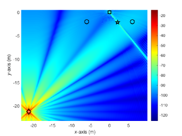
Figure 2: Enhanced beampattern of the RIS-assisted system (BS: diamond; RIS: square; target: star; users: circles).

VI-A Illustration of Radar Sensing Performance

We first visually demonstrate the communications and radar sensing functions by plotting the enhanced beampattern of the RIS-assisted ISAC system in Fig. 2. We clearly see that the BS generates strong beams towards the areas where the RIS, the target, and the users are located, meanwhile the RIS forms multiple passive beams to direct the signals towards the target and the users.

VI-B Convergence Performance of the Proposed Algorithms

We show the convergence performance of Algorithm 1 and Algorithm 2 in Figs. 3(a) and 3(b), respectively. The achievable sum-rate versus the number of iterations under different settings is presented to verify the convergence of our proposed algorithms. We observe that both Algorithm 1 and Algorithm 2 converge with 30 iterations.

VI-C Impact of Transmit Power

To verify the advantages of the proposed joint beamforming and reflection designs (denoted as “Proposed”), we also include the following schemes for comparisons.

• “Comm only”: Only the multi-user communication function is optimized for the considered system. The proposed joint beamforming and reflection design algorithm is utilized without considering the radar sensing constraint.

• “BF only”: With a fixed $\bm{\phi}$ which is determined by maximizing the sum channel gain, the beamformers $\mathbf{W}$ and $\mathbf{u}$ are iteratively solved for using Algorithm 1 for the SNR-constrained scenario, or $\mathbf{W}$ is iteratively solved for using Algorithm 2 for the CRB-constrained scenario.

• “Separate”: The reflection coefficients $\bm{\phi}$, the radar beamformer $\mathbf{W}_{\text{r}}$, the communication beamformer $\mathbf{W}_{\text{c}}$, and the receive filter $\mathbf{u}$ are separately optimized. In particular, $\bm{\phi}$ is obtained by maximizing the sum channel gain, $\mathbf{W}_{\text{r}}$ is determined by solving the power minimization problem under the radar SNR or CRB constraint, $\mathbf{W}_{\text{c}}$ is then designed by solving the sum-rate maximization problem under the power constraint, and finally for the SNR-constrained scenario $\mathbf{u}$ is given by (28).

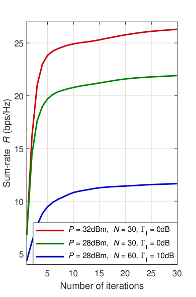
(a) Convergence of Algorithm 1.

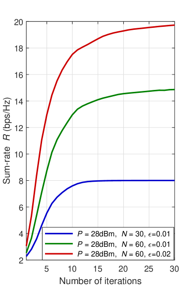
(b) Convergence of Algorithm 2.

Figure 3: Convergence performance of the proposed algorithms.

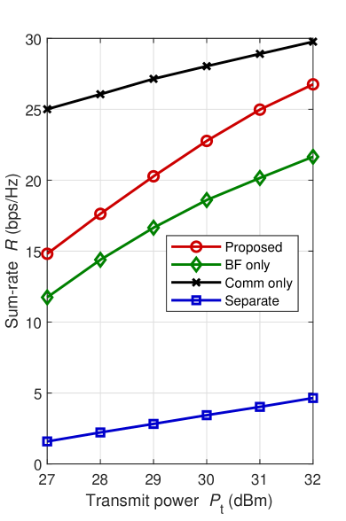
(a) SNR-constrained ($\Gamma_{\text{t}}=7$dB).

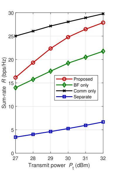
(b) CRB-constrained ($\varepsilon=0.02$).

Figure 4: Sum-rate versus transmit power $P_{\text{t}}$ ($N=49$).

The achievable sum-rate versus transmit power $P_{\text{t}}$ for the SNR-constrained joint beamforming and reflection design is presented in Fig. 4(a). We observe that the schemes which jointly design the radar and communication beamforming achieve a remarkable performance improvement compared with the “Separate” scheme. In addition, there is no doubt that the “Comm only” scheme achieves the best sum-rate performance and the proposed scheme is much better than the “BF only” scheme. Moreover, we observe that the performance gap between “Comm only” and the proposed scheme becomes smaller with the increase of $P_{\text{t}}$, since more transmit power can be exploited to improve the communication performance for a fixed radar sensing requirement. The performance of the CRB-constrained design is shown in Fig. 4(b), in which the same performance relationship as that for the SNR-constrained scenario is observed and similar conclusions can be drawn.

VI-D Impact of the Number of Reflecting Elements

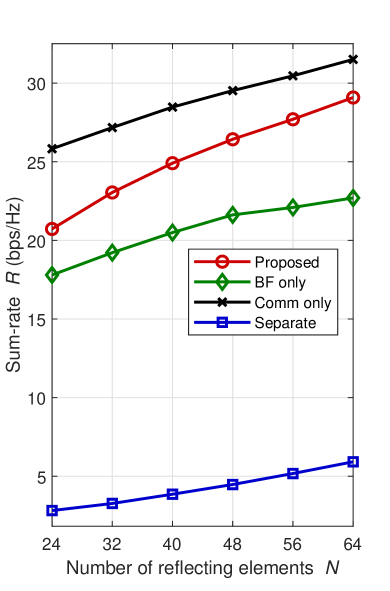
(a) SNR-constrained ($\Gamma_{\text{t}}=7$dB).

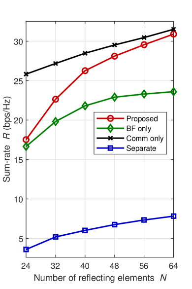
(b) CRB-constrained ($\varepsilon=0.02$).

Figure 5: Sum-rate versus the number of reflecting elements $N$ ($P=32$dBm).

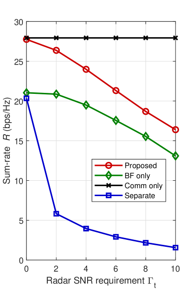
(a) $R$ versus SNR $\Gamma_{\text{t}}$.

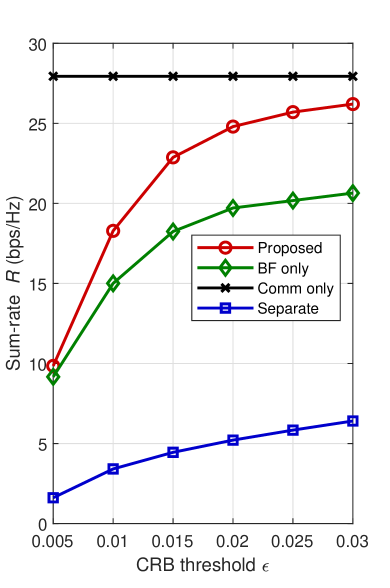
(b) $R$ versus CRB $\varepsilon$.

Figure 6: Impact of radar sensing performance ($N=49$, $P=30$dBm).

Next, we illustrate the achievable sum-rate versus the number of reflecting elements $N$ in Fig. 6. It is obvious that more reflecting elements provide larger passive beamforming gains since they can exploit more DoFs to manipulate the propagation environment. Moreover, comparing Fig. 5(a) and Fig. 5(b), we see that additional reflecting elements provide more pronounced performance gains for the CRB-constrained schemes. Specifically, the achievable sum-rate increases by 40% in the target detection scenario, and 76% in the target DoA estimation scenario. This phenomena implies that a larger RIS not only directs more energy to the target for detection, but more importantly, it improves the accuracy of the DoA estimation.

VI-E Impact of the Radar Sensing Performance

The impact of different radar sensing requirements is shown in Fig. 6. We clearly observe the performance trade-off between multi-user communications and radar target detection or DoA estimation. In addition, a huge performance degradation for the “Separate” scheme occurs when the radar SNR changes from 0dB to 2dB. This is because a tighter target detection constraint requires more power in designing $\mathbf{W}_{\text{r}}$, thus leaving less power for optimizing $\mathbf{W}_{\text{c}}$ to maximize the sum-rate.

VII Conclusions

In this paper, we considered a general case for RIS-assisted ISAC systems, in which both the direct and reflected links contribute to MU-MISO communications and radar sensing. In addition to the sum-rate performance metric for multi-user communications, we derived the radar SNR metric for target detection and the CRB for estimating target DoAs. We formulated the optimization problems that maximize the sum-rate as well as satisfy a worst-case radar SNR or CRB constraint, the transmit power budget, and the unit-modulus constraint of the RIS reflection coefficients. Efficient alternating algorithms based on FP, MM, and ADMM were developed to convert the resulting non-convex problems into several tractable sub-problems and then iteratively solve them. Simulation results verified the advantages of the proposed algorithms, illustrated the performance improvements introduced by more resources, and demonstrated the performance trade-off between communications and radar sensing with limited resources.

Appendix A

According to (17), the derivatives of $\bm{\eta}$ with respect to each parameter can be calculated as

$$\frac{\partial\bm{\eta}}{\partial\theta_{1}}=\alpha_{\text{t}}\text{vec}\{\dot{\mathbf{H}}_{\text{t}}(\bm{\phi})\mathbf{WS}\},~{}\frac{\partial\bm{\eta}}{\partial\theta_{2}}=\alpha_{\text{t}}\text{vec}\{\ddot{\mathbf{H}}_{\text{t}}(\bm{\phi})\mathbf{WS}\},~{}\frac{\partial\bm{\eta}}{\partial\bm{\alpha}}=[1~{}\jmath]^{T}\otimes\text{vec}\{{\mathbf{H}}_{\text{t}}(\bm{\phi})\mathbf{WS}\},$$ (66)

where $\dot{\mathbf{H}}_{\text{t}}(\bm{\phi})$ and $\ddot{\mathbf{H}}_{\text{t}}(\bm{\phi})$ denote the partial derivatives of $\mathbf{H}_{\text{t}}(\bm{\phi})$ with respect to $\theta_{1}$ and $\theta_{2}$, respectively. Thus, plugging (66) into (18), the elements of $\mathbf{F}_{\text{IM}}$ can be calculated as

$$F_{\theta_{1},\theta_{1}} =\frac{2|\alpha_{\text{t}}|^{2}}{\sigma_{\text{r}}^{2}}\Re\{\text{vec}^{H}\{\dot{\mathbf{H}}_{\text{t}}(\bm{\phi})\mathbf{WS}\}\text{vec}\{\dot{\mathbf{H}}_{\text{t}}(\bm{\phi})\mathbf{WS}\}\}=\frac{2L|\alpha_{\text{t}}|^{2}}{\sigma_{\text{r}}^{2}}\text{Tr}\{\dot{\mathbf{H}}_{\text{t}}(\bm{\phi})\mathbf{WW}^{H}\dot{\mathbf{H}}^{H}_{\text{t}}(\bm{\phi})\},$$ (67a)

$$F_{\theta_{1},\theta_{2}} =F_{\theta_{2},\theta_{1}}=\frac{2L|\alpha_{\text{t}}|^{2}}{\sigma_{\text{r}}^{2}}\Re\{\text{Tr}\{\ddot{\mathbf{H}}_{\text{t}}(\bm{\phi})\mathbf{WW}^{H}\dot{\mathbf{H}}^{H}_{\text{t}}(\bm{\phi})\}\},$$ (67b)

$$F_{\theta_{2},\theta_{2}} =\frac{2L|\alpha_{\text{t}}|^{2}}{\sigma_{\text{r}}^{2}}\text{Tr}\{\ddot{\mathbf{H}}_{\text{t}}(\bm{\phi})\mathbf{WW}^{H}\ddot{\mathbf{H}}^{H}_{\text{t}}(\bm{\phi})\},~{}~{}\mathbf{F}_{\bm{\alpha},\bm{\alpha}^{T}}=\frac{2L}{\sigma_{\text{r}}^{2}}\text{Tr}\{\mathbf{H}_{\text{t}}(\bm{\phi})\mathbf{WW}^{H}\mathbf{H}^{H}_{\text{t}}(\bm{\phi})\}\mathbf{I}_{2},$$ (67c)

$$\mathbf{F}_{\theta_{1},\bm{\alpha}^{T}} =\frac{2L}{\sigma_{\text{r}}^{2}}\Re\{\text{Tr}\{\alpha^{*}_{\text{t}}\mathbf{H}_{\text{t}}(\bm{\phi})\mathbf{WW}^{H}\dot{\mathbf{H}}^{H}_{\text{t}}(\bm{\phi})\}[1~{}\jmath]\},$$ (67d)

$$\mathbf{F}_{\theta_{2},\bm{\alpha}^{T}} =\frac{2L}{\sigma_{\text{r}}^{2}}\Re\{\text{Tr}\{\alpha^{*}_{\text{t}}\mathbf{H}_{\text{t}}(\bm{\phi})\mathbf{WW}^{H}\ddot{\mathbf{H}}^{H}_{\text{t}}(\bm{\phi})\}[1~{}\jmath]\}.$$ (67e)

It is noted that we assume that $\mathbf{SS}^{H}=L\mathbf{I}_{K}$ due to the fact that sufficient samples are usually collected for parameter estimation. Based on the above derivations, the sub-matrices of $\mathbf{F}$ can be constructed as

$$\mathbf{F}_{\bm{\theta}\bm{\theta}^{T}}=\left[\begin{array}[]{cc}F_{\theta_{1},\theta_{1}}&F_{\theta_{1},\theta_{2}}\\ F_{\theta_{2},\theta_{1}}&F_{\theta_{2},\theta_{2}}\end{array}\right],\quad\mathbf{F}_{\bm{\theta}\bm{\alpha}^{T}}=\left[\begin{array}[]{c}F_{\theta_{1},\bm{\alpha}^{T}}\\ F_{\theta_{2},\bm{\alpha}^{T}}\end{array}\right].$$ (68)

Appendix B

In order to re-arrange each element of $\mathbf{F}_{\text{IM}}$ as explicit expressions with respect to $\mathbf{W}$ and $\bm{\phi}$, we first utilize the transformation $\text{vec}\{\mathbf{ABC}\}=(\mathbf{C}^{T}\otimes\mathbf{A})\text{vec}\{\mathbf{B}\}$ to re-formulate the term $\mathbf{H}_{\text{t}}(\bm{\phi})\mathbf{w}_{k}$ as

$$\mathbf{H}_{\text{t}}(\bm{\phi})\mathbf{w}_{k}=\underbrace{\mathbf{h}_{\text{d,t}}\mathbf{h}_{\text{d,t}}^{T}\mathbf{w}_{k}}_{\mathbf{q}_{0,k}}+(\underbrace{\mathbf{w}_{k}^{T}\mathbf{h}_{\text{d,t}}\mathbf{G}^{T}\!\text{diag}\{\!\mathbf{h}_{\text{r,t}}\!\}\!+\!\mathbf{w}_{k}^{T}\mathbf{G}^{T}\!\text{diag}\{\!\mathbf{h}_{\text{r,t}}\!\}\!\otimes\!\mathbf{h}_{\text{d,t}}}_{\mathbf{U}_{0,k}})\bm{\phi}$$ (69)

$$\qquad\qquad\quad+(\underbrace{\mathbf{w}_{k}^{T}\mathbf{G}^{T}\!\text{diag}\{\mathbf{h}_{\text{r,t}}\}\!\otimes\!\mathbf{G}^{T}\!\text{diag}\{\mathbf{h}_{\text{r,t}}\}}_{\mathbf{Z}_{0,k}})\text{vec}\{\bm{\phi\phi}^{T}\!\}.$$

Similarly, the terms $\dot{\mathbf{H}}_{\text{t}}(\bm{\phi})\mathbf{w}_{k}$ and $\ddot{\mathbf{H}}_{\text{t}}(\bm{\phi})\mathbf{w}_{k}$ can be re-formulated as

$$\dot{\mathbf{H}}_{\text{t}}(\bm{\phi})\mathbf{w}_{k}=\mathbf{q}_{1,k}+\mathbf{U}_{1,k}\bm{\phi},\quad\ddot{\mathbf{H}}_{\text{t}}(\bm{\phi})\mathbf{w}_{k}=\mathbf{U}_{2,k}\bm{\phi}+\mathbf{Z}_{2,k}\text{vec}\{\bm{\phi\phi}^{T}\}.$$ (70)

Then, the functions $\mathcal{F}_{1}(\mathbf{W},\bm{\phi})\sim\mathcal{F}_{6}(\mathbf{W},\bm{\phi})$ are defined and re-arranged as

$$\mathcal{F}_{1}(\mathbf{W},\bm{\phi}) \triangleq\text{Tr}\{\dot{\mathbf{H}}_{\text{t}}(\bm{\phi})\mathbf{WW}^{H}\dot{\mathbf{H}}^{H}_{\text{t}}(\bm{\phi})\}=\sum_{k=1}^{K+M}\mathbf{w}_{k}^{H}\underbrace{\dot{\mathbf{H}}^{H}_{\text{t}}(\bm{\phi})\dot{\mathbf{H}}_{\text{t}}(\bm{\phi})}_{\mathbf{A}_{1}}\mathbf{w}_{k}$$

$$=\underbrace{\sum_{k=1}^{K+M}\mathbf{q}_{1,k}^{H}\mathbf{q}_{1,k}}_{q_{1}}+2\Re\Big{\{}\bm{\phi}^{H}\underbrace{\sum_{k=1}^{K+M}\mathbf{U}_{1,k}^{H}\mathbf{q}_{1,k}}_{\mathbf{u}_{1}}\Big{\}}+\bm{\phi}^{H}\underbrace{\sum_{k=1}^{K+M}\mathbf{U}_{1,k}^{H}\mathbf{U}_{1,k}}_{\mathbf{U}_{1}}\bm{\phi},$$ (71a)

$$\mathcal{F}_{2}(\mathbf{W},\bm{\phi}) \triangleq\text{Tr}\{\ddot{\mathbf{H}}_{\text{t}}(\bm{\phi})\mathbf{WW}^{H}\dot{\mathbf{H}}^{H}_{\text{t}}(\bm{\phi})\}=\text{Tr}\{\mathbf{A}_{2}\mathbf{WW}^{H}\}$$

$$=\overline{\mathbf{u}}_{2}^{H}\bm{\phi}+\bm{\phi}^{H}\mathbf{U}_{2}\bm{\phi}+\overline{\mathbf{z}}_{2}^{H}(\bm{\phi}\!\otimes\!\bm{\phi})+\bm{\phi}^{H}\mathbf{C}_{2}(\bm{\phi}\!\otimes\!\bm{\phi}),$$ (71b)

$$\mathcal{F}_{3}(\mathbf{W},\bm{\phi}) \triangleq\text{Tr}\{\mathbf{H}_{\text{t}}(\bm{\phi})\mathbf{WW}^{H}\dot{\mathbf{H}}^{H}_{\text{t}}(\bm{\phi})\}=\text{Tr}\{\mathbf{A}_{3}\mathbf{WW}^{H}\}$$

$$=q_{3}+\bm{\phi}^{H}\mathbf{u}_{3}+\overline{\mathbf{u}}_{3}^{H}\bm{\phi}+\bm{\phi}^{H}\mathbf{U}_{3}\bm{\phi}+\overline{\mathbf{z}}_{3}^{H}(\bm{\phi}\!\otimes\!\bm{\phi})+\bm{\phi}^{H}\mathbf{C}_{3}(\bm{\phi}\!\otimes\!\bm{\phi}),$$ (71c)

$$\mathcal{F}_{4}(\mathbf{W},\bm{\phi}) \triangleq\text{Tr}\{\ddot{\mathbf{H}}_{\text{t}}(\bm{\phi})\mathbf{WW}^{H}\ddot{\mathbf{H}}^{H}_{\text{t}}(\bm{\phi})\}=\text{Tr}\{\mathbf{A}_{4}\mathbf{WW}^{H}\}$$

$$=\bm{\phi}^{H}\mathbf{U}_{4}\bm{\phi}+2\Re\big{\{}(\bm{\phi}\!\otimes\!\bm{\phi})^{H}\overline{\mathbf{C}}_{4}\bm{\phi}\big{\}}+(\bm{\phi}\!\otimes\!\bm{\phi})^{H}\mathbf{Z}_{4}(\bm{\phi}\!\otimes\!\bm{\phi}),$$ (71d)

$$\mathcal{F}_{5}(\mathbf{W},\bm{\phi}) \triangleq\text{Tr}\{\mathbf{H}_{\text{t}}(\bm{\phi})\mathbf{WW}^{H}\ddot{\mathbf{H}}^{H}_{\text{t}}(\bm{\phi})\}=\text{Tr}\{\mathbf{A}_{5}\mathbf{WW}^{H}\}=\bm{\phi}^{H}\mathbf{u}_{5}+\bm{\phi}^{H}\mathbf{U}_{5}\bm{\phi}+(\bm{\phi}\!\otimes\!\bm{\phi})^{H}\mathbf{z}_{5}$$

$$\quad+(\bm{\phi}\!\otimes\!\bm{\phi})^{H}\mathbf{Z}_{5}(\bm{\phi}\!\otimes\!\bm{\phi})+(\bm{\phi}\!\otimes\!\bm{\phi})^{H}\overline{\mathbf{C}}_{5}\bm{\phi}+\bm{\phi}^{H}\mathbf{C}_{5}(\bm{\phi}\!\otimes\!\bm{\phi}),$$ (71e)

$$\mathcal{F}_{6}(\mathbf{W},\bm{\phi}) \triangleq\text{Tr}\{\mathbf{H}_{\text{t}}(\bm{\phi})\mathbf{WW}^{H}\mathbf{H}^{H}_{\text{t}}(\bm{\phi})\}=\text{Tr}\{\mathbf{A}_{6}\mathbf{WW}^{H}\}=q_{6}+2\Re\big{\{}\bm{\phi}^{H}\mathbf{u}_{6}\big{\}}+\bm{\phi}^{H}\mathbf{U}_{6}\bm{\phi}$$

$$\quad+2\Re\big{\{}(\bm{\phi}\!\otimes\!\bm{\phi})^{H}\mathbf{z}_{6}\big{\}}+(\bm{\phi}\!\otimes\!\bm{\phi})^{H}\mathbf{Z}_{6}(\bm{\phi}\!\otimes\!\bm{\phi})+2\Re\big{\{}(\bm{\phi}\!\otimes\!\bm{\phi})^{H}\overline{\mathbf{C}}_{6}\bm{\phi}\big{\}}.$$ (71f)

Considering that the derivations are similar and straightforward, we only present the detailed derivations and expressions for $\mathcal{F}_{1}(\mathbf{W},\bm{\phi})$. The details for other variables irrelevant to $\bm{\phi}$ can be obtained in the same way and are omitted in this paper due to space limitations.

References

• [1] R. Liu, M. Li, and A. L. Swindlehurst, “Joint beamforming and reflection design for RIS-assisted ISAC systems,” in Proc. European Signal Process., Belgrade, Serbia, Aug. 2022.
• [2] F. Liu, C. Masouros, A. P. Petropulu, H. Griffiths, and L. Hanzo, “Joint radar and communication design: Applications, state-of-the-art, and the road ahead,” IEEE Trans. Commun., vol. 68, no. 6, pp. 3834-3862, Jun. 2020.
• [3] J. A. Zhang, M. L. Rahman, K. Wu, X. Huang, Y. J. Guo, S. Chen, and J. Yuan, “Enabling joint communication and radar sensing in mobile networks - A survey,” IEEE Commun. Surveys Tuts., vol. 24, no. 1, pp. 306-345, First Quart. 2022.
• [4] F. Liu, Y. Cui, C. Masouros, J. Xu, T. X. Han, Y. C. Eldar, and S. Buzzi, “Integrated sensing and communications: Towards dual-functional wireless networks for 6G and beyond,” IEEE J. Sel. Areas Commun., vol. 40, no. 6, pp. 1728-1767, Jun. 2022.
• [5] A. Liu, et al., “A survey on fundamental limits of integrated sensing and communication,” IEEE Commun. Surveys Tuts., vol. 24, no. 2, pp. 994-1034, 2nd Quart. 2022.
• [6] F. Liu, et al., “Seventy years of radar and communications: The road from separation to integration,” Oct. 2022. [Online]. Available: https://arxiv.org/abs/2210.00446v1
• [7] X. Liu, T. Huang, N. Shlezinger, Y. Liu, J. Zhou, and Y. C. Eldar, “Joint transmit beamforming for multiuser MIMO communications and MIMO radar,” IEEE Trans. Signal Process., vol. 68, pp. 3929-3944, Jun. 2020.
• [8] J. A. Zhang, F. Liu, C. Masouros, R. W. Heath Jr., Z. Feng, L. Zheng, and A. Petropulu, “An overview of signal processing techniques for joint communication and radar sensing,” IEEE J. Sel. Topics Signal Process., vol. 15, no. 6, pp. 1295-1315, Nov. 2021.
• [9] F. Liu, Y.-F. Liu, A. Li, C. Masouros, and Y. C. Eldar, “Cramér-Rao bound optimization for joint radar-communication beamforming,” IEEE Trans. Signal Process., vol. 70, pp. 240-253, Dec. 2021.
• [10] B. K. Chalise, M. G. Amin, and B. Himed, “Performance tradeoff in a unified passive radar and communications system,” IEEE Signal Process. Lett., vol. 24, no. 9, pp. 1275-1279, Sep. 2017.
• [11] H. Hua, T. X. Han, and J. Xu, “MIMO integrated sensing and communication: CRB-rate tradeoff,” Sep. 2022. [Online]. Available: https://arxiv.org/abs/2209.12721v1
• [12] R. Liu, M. Li, Q. Liu, and A. L. Swindlehurst, “Joint waveform and filter designs for STAP-SLP-based MIMO-DFRC systems,” IEEE J. Sel. Areas Commun., vol. 40, no. 6, pp. 1918-1931, Jun. 2022.
• [13] M. Di Renzo et al., “Smart radio environments empowered by reconfigurable intelligent surfaces: How it works, state of research, and the road ahead,” IEEE J. Sel. Areas Commun., vol. 38, no. 11, pp. 2450-2525, Nov. 2020.
• [14] Q. Wu, S. Zhang, B. Xiong, C. You, and R. Zhang, “Intelligent reflecting surface aided wireless communications: A tutorial,” IEEE Trans. Commun., vol. 69, no. 5, pp. 3313-3351, May 2021.
• [15] E. Ayanoglu, F. Capolino, and A. L. Swindlehurst, “Wave-controlled metasurface-based reconfigurable intelligent surfaces,” IEEE Wireless Commun., vol. 29, no. 4, pp. 86-92, Aug. 2022.
• [16] Q. Wu and R. Zhang, “Intelligent reflecting surface enhanced wireless network via joint active and passive beamforming,” IEEE Trans. Wireless Commun., vol. 18, no. 11, pp. 5394-5409, Nov. 2019.
• [17] R. Liu, M. Li, Q. Liu, and A. Lee Swindlehurst, “Joint symbol-level precoding and reflecting designs for IRS-enhanced MU-MISO systems,” IEEE Trans. Wireless Commun., vol. 20, no. 2, pp. 798-811, Feb. 2021.
• [18] X. Song, J. Xu, F. Liu, T. X. Han, and Y. C. Eldar, “Intelligent reflecting surface enabled sensing: Cramér-Rao bound optimization,” in IEEE Globecom Workshops (GC Wkshps), Rio de Janeiro, Brazil, Dec. 2022.
• [19] R. Liu, M. Li, H. Luo, Q. Liu, and A. L. Swindlehurst, “Integrated sensing and communication with reconfigurable intelligent surfaces: Opportunities, applications, and future directions,” IEEE Wireless Commun., to appear.
• [20] S. P. Chepuri, N. Shlezinger, F. Liu, G. C. Alexandropoulos, S. Buzzi, and Y. C. Eldar, “Integrated sensing and communications with reconfigurable intelligent surfaces,” Nov. 2022. [Online]. Available: https://arxiv.org/abs/2211.01003v1
• [21] X. Wang, Z. Fei, Z. Zheng, and J. Guo, “Joint waveform design and passive beamforming for RIS-assisted dual-functional radar-communication system,” IEEE Trans. Veh. Technol., vol. 70, no. 5, pp. 5131-5136, May 2021.
• [22] X. Wang, Z. Fei, J. Huang, and H. Yu, “Joint waveform and discrete phase shift design for RIS-assisted integrated sensing and communication system under Cramér-Rao bound constraint,” IEEE Trans. Veh. Technol., vol. 71, no. 1, pp. 1004-1009, Jan. 2022.
• [23] H. Luo, R. Liu, M. Li, Y. Liu, and Q. Liu, “Joint beamforming design for RIS-assisted integrated sensing and communication systems,” IEEE Trans. Veh. Technol., vol. 71, no. 12, pp. 13393-13397, Dec. 2022.
• [24] X. Song, T. X. Han, and J. Xu, “Cramér-Rao bound minimization for IRS-enabled multiuser integrated sensing and communication with extended target,” Oct. 2022. [Online]. Available: https://arxiv.org/abs/2210.16592v1
• [25] Z. Xing, R. Wang, and X. Yuan, “Passive beamforming design for reconfigurable intelligent surface enabled integrated sensing and communication,” Jun. 2022. [Online]. Available: https://arxiv.org/abs/2206.00525v1
• [26] Z. Wang, X. Mu, and Y. Liu, “STARS enabled integrated sensing and communications,” Jul. 2022. [Online]. Available: https://arxiv.org/abs/2207.10748v1
• [27] S. Yan, S. Cai, W. Xia, J. Zhang, and S. Xia, “A reconfigurable intelligent surface aided dual-function radar and communication system,” in Proc. IEEE Int. Symp. Joint Commun. Sensing (JC&S), Seefeld, Austria, Mar. 2022.
• [28] R. Liu, M. Li, Y. Liu, Q. Wu, and Q. Liu, “Joint transmit waveform and passive beamforming design for RIS-aided DFRC systems,” IEEE J. Sel. Topics Signal Process., vol. 16, no. 5, pp. 995-1010, Aug. 2022.
• [29] C. Hu, L. Dai, S. Han, and X. Wang, “Two-timescale channel estimation for reconfigurable intelligent surface aided wireless communications,” IEEE Trans. Commun., vol. 69, no. 11, pp. 7736-7747, Nov. 2021.
• [30] S. M. Kay, Fundamentals of Statistical Signal Processing: Detection Theory, vol. 2. Englewood Cliffs, NJ, USA: Prentice-Hall, 1998.
• [31] I. Bekkerman and J. Tabrikian, “Target detection and localization using MIMO radars and sonars,” IEEE Trans. Signal Process., vol. 54, no. 10, pp. 3873-3883, Oct. 2006.
• [32] S. M. Kay, Fundamentals of Statistical Signal Processing: Estimation Theory, vol. 1, Englewood Cliffs, NJ, USA: Prentice Hall, 1998.
• [33] K. Shen and W. Yu, “Fractional programming for communication systems-part I: Power control and beamforming,” IEEE Trans. Signal Process., vol. 66, no. 10, pp. 2616-2630, May. 2018.
• [34] S. Boyd, S. P. Boyd, and L. Vandenberghe, Convex optimization. Cambridge, U.K.: Cambridge university press, 2004.
• [35] F. Zhang, The Schur Complement and Its Applications. Berlin, Germany: Springer-Verlag, 2005.