Klein-Gordon Equation with Self-Interaction $\lambda\phi^{4}$ and Arbitrary Spherical Source Terms

Abstract

The Klein-Gordon equation for a scalar field sourced by a spherically symmetric background is an interesting second-order differential equation with applications in particle physics, astrophysics, and elsewhere. Here we present solutions for generic source density profiles in the case where the scalar field has no interactions or a mass term. For a $\lambda\phi^{4}$ self-interaction term, we provide the necessary expressions for a numerical computation, an algorithm to numerically match the initial conditions from infinity to the origin, and an accurate guess of that initial condition. We also provide code to perform the numerical calculations that can be adapted for arbitrary density profiles.

I Introduction

The Klein-Gordon equation allows one to compute the behavior of a relativistic field $\phi(t,x,y,z)$. The massless form with no interactions is

$$\square\phi=0\,,$$ (1)

where $\square$ is the d’Alembert operator $\square=\frac{\partial^{2}}{\partial t^{2}}-\frac{\partial^{2}}{\partial x^{2}}-\frac{\partial^{2}}{\partial y^{2}}-\frac{\partial^{2}}{\partial z^{2}}$. The more general version of the Klein-Gordon equation includes a mass term for $\phi$ as well as additional interactions.

$$\square\phi+V^{\prime}(\phi)=0\,,$$ (2)

where $V$ is the potential and the prime denotes the derivative with respect to the field. The potential for a massive field that is also self interacting is

$$V(\phi)=\frac{1}{2}m^{2}\phi^{2}+\frac{1}{4!}\lambda\phi^{4}\,,$$ (3)

where $m$ is the mass of the field and $\lambda$ is a dimensionless parameter of the model indicating the strength of the interaction. Such a potential has been considered in many different physical environments including loops, renormalization effects, sources, and perturbative solutions among others, see e.g. Coleman and Weinberg (1973); Dvali et al. (2011); Yoda and Nojiri (2012); Shi (2021); Davoudiasl and Denton (2023). Note that a $\phi^{4}$ term may be induced at the loop level or may contribute to loop calculations. We ignore these issues here and treat $\phi$ as a classical field which is relevant when $\lambda\ll 1$. In addition, one could also consider a cubic term $\propto\phi^{3}$ which we also ignore as it turns out the $\lambda\phi^{4}$ term will contain all the challenges of the more general potential. Finally, we note that we are fixing the signs of the terms in eq. 3; the Higgs field is a well studied example with a different sign on the $m^{2}\phi^{2}$ term. The numerical approach is equally valid in either case, while care is required to extend the analytic results.

The final contribution to the Klein-Gordon equation we consider is a source term $n(r)$ where $n(r)$ is some background field charge density profile that is coupled to $\phi$ via an additional interaction. We also assume that $n(r)=0$ for $r>r_{s}$ where $r_{s}$ is the finite radius of the object. Note that we have taken $n$ to be spherically symmetric and depend only on the radius and not direction or time. We will also assume that $\lim_{r\to 0}n(r)$ is finite. These conditions are all met for celestial objects such as planets or stars. Now the full Klein-Gordon equation we will consider is

$$\square\phi+m^{2}\phi+\frac{1}{3!}\lambda\phi^{3}+n(r)=0\,.$$ (4)

Since the equation is independent of time or direction in spherical coordinates, we make the ansatz that $\phi(t,x,y,z)=\phi(r)$. Then, in spherical coordinates, we have the second order differential equation we wish to solve:

$$-2\frac{\phi^{\prime}}{r}-\phi^{\prime\prime}+m^{2}\phi+\frac{1}{3!}\lambda\phi^{3}+n(r)=0\,,$$ (5)

where the primes denote derivatives with respect to $r$.

Before we begin to solve it, we note several features.

• Being a second order differential equation, two initial conditions are necessary (but not necessarily sufficient) to uniquely determine the field. The initial conditions will depend on the underlying physics of the problem, outlined here.

• The first of the initial conditions can be determined at the center of the sphere where symmetry arguments find that we must have $\phi^{\prime}(0)=0$, provided that $\phi$ is $C^{1}$ through the origin. Diverging derivatives would require that the field diverges so this possibility can be discarded, provided that a finite solution can be found.

• Next, we have that the field should satisfy $\phi(\infty)=0$ since in the absence of a source term we want the field to return to the vacuum state.

• The inclusion of the $\lambda$ term makes the equation non-linear. Thus one cannot use superposition to take a single solution and form up the total solution as one can in the case where $\lambda=0$.

Before addressing the full solution in its generality, we solve it in simpler cases and learn useful strategies for the full solution.

II Massless Non-Self Interacting Case

We begin with the simplest possible case: $m=\lambda=0$. The differential equation is

$$-2\frac{\phi^{\prime}}{r}-\phi^{\prime\prime}+n(r)=0\,.$$ (6)

This is equivalent to electrodynamics and can be solved in many ways. We focus on deriving a general solution to the differential equation.

The solution for $r>r_{s}$ is

$$\phi(r)=\frac{A}{r}+B\,,$$ (7)

for free parameters $A$ and $B$. We see that $B=0$ since $\phi(\infty)=0$.

Inside the sphere the general solution is

$$\phi(r)=C+\int_{0}^{r}\left(\frac{D}{r_{1}^{2}}+\frac{g}{r_{1}^{2}}\int_{0}^{r_{1}}n(r_{2})r_{2}^{2}dr_{2}\right)dr_{1}\,,$$ (8)

for some free parameters $C$ and $D$. From the initial condition $\phi^{\prime}(0)=0$ we must have $D=0$.

It is useful to know $\phi(0)$ for numerical purposes. We calculate $\lim_{r\to 0}\phi(r)$ directly from the differential equation, eq. 6, by multiplying by $r$ (this does not create a problem for evaluation as $r\to 0$ since $\phi\in C^{1}$) and integrating over $r$:

$$-2\int_{0}^{\infty}\phi^{\prime}dr-\int_{0}^{\infty}r\phi^{\prime\prime}dr+\int_{0}^{r_{s}}n(r)rdr=0\,.$$ (9)

We now use the fact that $\lim_{r\to\infty}r\phi^{\prime}(r)=0$ since $\phi^{\prime}(r)$ must fall off faster than $1/r$ as $r\to\infty$ since if $\phi^{\prime}(r)\to 1/r$ then $\phi(r)\to\log(r)$ at large $r$ diverges which fails our second initial condition requirement. We also use $\phi^{\prime}(0)=0$ and find that

$$\phi(0)=-\int_{0}^{r_{s}}rn(r)dr\,.$$ (10)

This allows for a determination of $C$ in eq. 8. Combining eq. 10 with eq. 8 for $r<r_{s}$, we have

$$\phi(r)=\int_{0}^{r}\left(\frac{1}{r_{1}^{2}}\int_{0}^{r_{1}}n(r_{2})r_{2}^{2}dr_{2}\right)dr_{1}-\int_{0}^{r_{s}}n(r_{1})r_{1}dr_{1}\,.$$ (11)

Finally we determine $A$ in eq. 7 to be

$$A=-gr_{s}\int_{0}^{r_{s}}\left(n(r)r-\frac{1}{r^{2}}\int_{0}^{r}n(r_{1})r_{1}^{2}dr_{1}\right)dr\,,$$ (12)

completing the calculation.

II.1 An Example

A common example is to consider a uniform hard sphere of charge given by

$$n(r)=\begin{cases}n\qquad&r<r_{s}\\ 0&r>r_{s}\end{cases}\,.$$ (13)

While astrophysical bodies typically have $n^{\prime}(r)\lneq 0$ for $r<r_{s}$, this approximation may still be useful for showing the behavior of the field from a large core sourcing most of the field strength.

We show that these equations reproduce the known behavior. First we find that

$$A=-\frac{1}{3}nr_{s}^{3}\,,$$ (14)

We define the total charge

$$Q =4\pi\int_{0}^{r_{s}}n(r)r^{2}dr\,,$$ (15)

$$=\frac{4}{3}\pi nr_{s}^{3}\,,$$ (16)

where for the second equation we have set $n(r)$ to the step function in eq. 13. Then the solution reproduces the familiar result

$$\phi(r)=\begin{cases}-\frac{Q}{8\pi r_{s}}\left(3-\frac{r^{2}}{r_{s}^{2}}\right)\qquad&r<r_{s}\\ -\frac{Q}{4\pi r}&r>r_{s}\end{cases}\,.$$ (17)

III Massive Non-Self Interacting Case

We now consider $m\neq 0$ but still keep $\lambda=0$. This is often referred to as a Yukawa potential Yukawa (1935). The differential equation is

$$-2\frac{\phi^{\prime}}{r}-\phi^{\prime\prime}+m^{2}\phi+n(r)=0\,,$$ (18)

which has also been studied in a variety of contexts including with the spherical source term Yukawa (1935); Smirnov and Xu (2019).

For $r>r_{s}$ the solution is

$$\phi(r)=\frac{A}{r}e^{-mr}+\frac{B}{r}e^{mr}\,,$$ (19)

for free parameters $A$ and $B$. Again, $B=0$ since $\phi(\infty)=0$ and we have taken $m>0$ WLOG.

Inside the sphere the solution is of the form

$$\phi(r)=\frac{C}{r}e^{-mr}+\frac{D}{r}e^{mr}+I(r)\,,$$ (20)

where

$$I(r) =\frac{g}{2mr}\left[e^{mr}\int_{0}^{r}e^{-mr_{1}}n(r_{1})r_{1}dr_{1}-e^{-mr}\int_{0}^{r}e^{mr_{1}}n(r_{1})r_{1}dr_{1}\right]\,,$$ (21)

$$I^{\prime}(r) =\frac{-g}{2mr^{2}}\left[e^{mr}(1-mr)\int_{0}^{r}e^{-mr_{1}}n(r_{1})r_{1}dr_{1}-e^{-mr}(1+mr)\int_{0}^{r}e^{mr_{1}}n(r_{1})r_{1}dr_{1}\right]\,.$$ (22)

Note that $\lim_{r\to 0}I^{\prime}(r)=0$ so long as $n(r)$ is finite at the origin. To satisfy the initial condition $\phi^{\prime}(0)=0$ we must have $C=-D$. Then we write

$$\phi(r)=2\frac{D}{r}\sinh(mr)+I(r)\,,$$ (23)

We now require that $\phi$ and $\phi^{\prime}$ are continuous at $r=r_{s}$. We find

$$A={} I(r_{s})r_{s}\cosh(mr_{s})$$

$$-\frac{1}{m}\left[I(r_{s})+I^{\prime}(r_{s})r_{s}\right]\sinh(mr_{s})\,,$$ (24)

$$D={} -\frac{e^{-mr_{s}}}{2m}\left[I(r_{s})(1+mr_{s})+I^{\prime}(r_{s})r_{s}\right]\,.$$ (25)

Thus $I(r)$ and $I^{\prime}(r)$ contain all the non-trivial information about $n(r)$ necessary to compute $\phi(r)$ anywhere. This completes the calculation.

III.1 An Example

We again repeat the example of the previous section where $n(r)$ is a hard sphere as defined in eq. 13. Then we have

$$I(r) =\frac{n}{m^{3}r}\left[\sinh(mr)-mr\right]\,,$$ (26)

$$I^{\prime}(r) =-\frac{n}{m^{3}r^{2}}\left[\sinh(mr)-mr\cosh(mr)\right]\,.$$ (27)

This leads to coefficients of

$$A =\frac{n}{m^{3}}\left[\sinh(mr_{s})-mr_{s}\cosh(mr_{s})\right]\,,$$ (28)

$$D =-\frac{n}{2m^{3}}\left[1-e^{-mr_{s}}-mr_{s}e^{-mr_{s}}\right]\,.$$ (29)

Thus we write the complete solution for the hard sphere of charge as

$$\phi(r)=\\ \begin{cases}-\frac{n}{m^{2}}\left[1-e^{-mr_{s}}(1+mr_{s})\frac{\sinh(mr)}{mr}\right]&r<r_{s}\\ -\frac{n}{m^{2}}\left[mr_{s}\cosh(mr_{s})-\sinh(mr_{s})\right]\frac{e^{-mr}}{mr}&r>r_{s}\end{cases}\,.$$ (30)

It is easy to verify that this recovers the massless solution in the limit $m\to 0$.

Analytic expressions also exist for some other density profiles such an exponential density function of the form $n(r)=n_{0}e^{-r\kappa}$, see e.g. Smirnov and Xu (2019).

III.2 Beyond a point charge

The above solution is for a hard sphere of charge, we now elaborate some of its properties. First, in the limit that $r_{s}$ is small compared to $1/m$, but $n/r_{s}^{3}$ proportional to the total charge $Q$ defined in eq. 15 is held constant, we find that we recover the expected Yukawa potential expression valid for $r\gg r_{s}$

$$\lim_{r_{s}\to 0}\phi(r)=-\frac{Q}{4\pi}\frac{e^{-mr}}{r}\,.$$ (31)

If we add in the next terms in the $mr_{s}\ll 1$ expansion, we find

$$\phi(r)=-\frac{Q}{4\pi}\frac{e^{-mr}}{r}\left\{1\vphantom{\frac{1}{2}}\right.\\ \left.+\frac{1}{10}\left(mr_{s}\right)^{2}+\frac{1}{280}\left(mr_{s}\right)^{4}+\mathcal{O}[(mr_{s})^{6}]\right\}\,.$$ (32)

Thus a Yukawa potential for a massive mediator depends not only on the total charge of the source, but also the size of the source. Note that linearity applies here since $\lambda=0$ so a non-uniform source can be summed or integrated.

We see from eq. 32 that if $mr_{s}\sim 1$ then there is a $\sim 10\%$ correction to the point charge assumption, and it takes only $mr_{s}\sim 3$ to get a factor of 2 correction from the point charge approximation. Objects with a declining density profile $n^{\prime}(r)<0$ will see a smaller correction as they are closer to a point charge.

III.3 Surface to Core Ratio

A quantity that may be of interest for some problems is the ratio of the field strength at the surface of the sphere to the center. Continuing with $\lambda=0$, for limiting values of $m$ we find that the ratio is

$$R_{sc}\equiv\frac{\phi(r_{s})}{\phi(0)}=\begin{cases}\dfrac{\int_{0}^{r_{s}}r^{2}n(r)dr}{r_{s}\int_{0}^{r_{s}}rn(r)dr}\quad&m=0\\[14.45377pt] \dfrac{1}{2}\dfrac{n(r_{s})}{n(0)}&m\to\infty\end{cases}\,,$$ (33)

where the $\frac{1}{2}$ comes from assume that we are exactly at $r=r_{s}$. In the hard sphere case this simplifies to

$$R_{sc}=\frac{\sinh(mr_{s})-mr_{s}\cosh(mr_{s})}{mr_{s}-e^{mr_{s}}+(mr_{s})^{2}}\,,$$ (34)

which is, in the limits,

$$R_{sc}=\begin{cases}\frac{2}{3}\quad&m=0\\[7.22743pt] \frac{1}{2}&m\to\infty\end{cases}\,,$$ (35)

but has a local minimum at $mr_{s}\simeq 3.93$ where $R_{sc}\simeq 0.41$. So the allowed range of $R_{sc}$ for any value of $m$ but with $\lambda=0$ is $[0.41,\frac{2}{3}]$.

We note that so long as $n^{\prime}(r)<0$ (which is what we expect in celestial situations), then $R_{sc}\lneq\frac{2}{3}$ at $m=0$. Similarly, in the $m\to\infty$ limit $R_{sc}\lneq\frac{1}{2}$.

IV Massive Self Interacting Case

We now address the solution of the full differential equation from eq. 5 including the $\lambda\phi^{3}$ term. We are not aware of a general analytic solution to this equation. Ref. Frasca (2011) determined the time and space varying wave solution in the absence of a source term. To understand the behavior of the full equation we turn to approximations and numerical solutions.

We begin by identifying several useful properties of this equation to aid in numerical solutions. First, we note that the term $\phi^{\prime}/r$ becomes $0/0$ as $r\to 0$. In the limit $r\to 0$, since $\phi^{\prime}(0)=0$, we have that $\phi^{\prime\prime}(0)=\lim_{r\to 0}\phi^{\prime}(r)/r$ by L’Hôpital’s rule. Thus

$$\lim_{r\to 0}\frac{\phi^{\prime}(r)}{r}=\frac{1}{3}\left[m^{2}\phi(0)+\frac{\lambda}{3!}\phi^{3}(0)+n(0)\right]\,.$$ (36)

Thus all that is needed to determine this ratio is $\phi(0)$. Moreover, $\phi(0)$ is also needed to have both initial conditions at the origin (the other being $\phi^{\prime}(0)=0$) and allows us to calculate eq. 36 to evaluate the differential equation near the origin.

The value of $\phi(0)$ is ultimately set from the fact that $\phi(\infty)=0$. In principle, one can numerically vary $\phi(0)$ until one finds that $\phi(\infty)\to 0$. This strategy is numerically viable by following a procedure that maximizes the distance $r$ at which either $\phi(r)$ crosses zero or when the derivative changes from positive to negative.

This strategy suffers from two main problems. First, a sufficiently accurate initial guess is needed to realistically converge on the correct value of $\phi(0)$. Second, when $\lambda$ is large enough to contribute, the differential equation may become quite stiff depending on the shape of the density profile. For example, for some interesting parameters, we find that changing the initial condition $\phi(0)$ by one part in the $10^{14}$, close to the doule precision limit, the numerical solution varies between diverging to positive infinity and negative infinity well within $r_{s}$. Thus we find that while it may be possible to evaluate $\phi(0)$ to good precision, it is not always sufficient to fully evolve the function to any value of $r$ desired. Arbitrary precision techniques are likely required here.

To aid with the first issue, we found some expressions that serve well to approximate $\phi(0)$ by examining its behavior in different limits and then connecting them together. In the small $\lambda$ limit we recover the solution from eqs. 23 and 25 which is

$$\lim_{\lambda\to 0}\phi(0) =-e^{-mr_{s}}\left[I(r_{s})(1+mr_{s})+I^{\prime}(r_{s})r_{s}\right]$$ (37)

$$\equiv f_{0}$$ (38)

In the hard sphere case, this becomes

$$\lim_{\lambda\to 0}\phi(0)=-\frac{n}{m^{2}}\left[1-e^{-mr_{s}}(1+mr_{s})\right]\,.$$ (39)

In the massless case this returns the known result,

$$\lim_{\lambda,m\to 0}\phi(0)=-\frac{nr_{s}^{2}}{2}\,.$$ (40)

Second, we consider $\phi(0)$ in the large $\lambda$ limit,

$$\lim_{\lambda\to\infty}\phi(0) =-\left[\frac{3!}{\lambda}n(0)\right]^{1/3}$$ (41)

$$\equiv f_{\infty}(\lambda)$$ (42)

Then to interpolate between the two, we numerically use this functional form

$$\phi(0)\simeq-\left[|f_{0}|^{-\alpha}+|f_{\infty}(\lambda)|^{-\alpha}\right]^{-1/\alpha}\,,$$ (43)

where we find that $\alpha=2$ provides good numerical agreement as shown in fig. 1. In particular, we can numerically determine the optimal value of $\alpha$ over an interesting range of $\lambda$ and find that $\alpha\simeq 1.97$ at $m=0$ which then increases to $\alpha\simeq 2.38$ at $m=1$ and then decreases back down below $2$ as $m$ continues to increase. This justifies our choice of $\alpha=2$ as a good guess for all cases.

We also note that in the hard sphere case we find the critical value of $\lambda$ that indicates when the transition between the two limits occurs.

$$\lambda_{c}=\frac{3!}{n^{2}}\left(\frac{m^{2}}{1-e^{-mr_{s}}(1+mr_{s})}\right)^{3}\,,$$ (44)

which, in the massless limit, becomes

$$\lim_{m\to 0}\lambda_{c}=\frac{3!\times 2^{3}}{n^{2}r_{s}^{6}}\,.$$ (45)

We see in fig. 1 that eq. 43 is accurate at the $\lesssim 1-2\%$ level for $m=0$ and $\lesssim 10\%$ when both $m$ and $\lambda$ are contributing. This is sufficient to guess the initial value of $\phi(0)$ in the hard shell case and can be used to derive a useful guess for arbitrary density profiles.

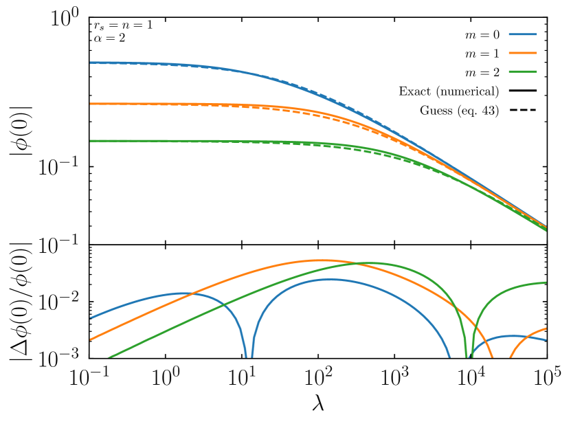
Figure 1: Top: The numerical value of $|\phi(0)|$ as a function of $\lambda$ for different representative values of $m$. The dashed curves are the approximations using eq. 43. We use a hard sphere of charge with $n=1$ and $r_{s}=1$ and fix $\alpha=2$. Bottom: The fractional error between the exact numerical and approximate calculations.

In fig. 2 we show the value of the field as a function of radius for various different values of $m$ and $\lambda$ in the hard sphere of charge case, normalized to the field strength at the origin for easy comparison. We see that in the case with $m\neq 0$ and $\lambda=0$ (Yukawa) the field falls to zero faster than in the $m=\lambda=0$ (electromagnetic) case, as expected due to the $e^{-mr}$ contribution. The inclusion of the self-interacting $\lambda$ term, however, causes the field to fall off back to zero more slowly at first, and then faster later, leading to a distinct behavior that cannot be recovered with just $m$. We also see that at large $r$ the $m$ term will dominate over the $\lambda$ term. This makes sense since as $r$ increases, $|\phi|$ decreases and thus the contribution from $\frac{\lambda}{3!}\phi^{3}$ will decrease relative to the $m^{2}\phi$ term.

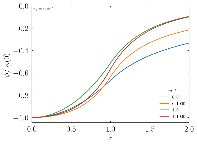
Figure 2: The normalized field value for four different pairs of $m$ and $\lambda$ as a function of radius in the hard sphere of charge case. We have taken the sphere size to be unity $r_{s}=1$ and the density to also be unity $n=1$.

V Code

We provide code to numerically compute solutions to the Klein-Gordon equation in for arbitrary spherically symmetric source potentials Denton (2023). The primary calculations occur in the S5.cpp file. The code evaluates $\phi(0)$ with the phi0_KG function using the phi0_Guess function as a guess. Some care may be required to get an appropriate window, depending on the parameters used and the density profile. Three density profiles are included: HARD, SUN from BS05(OP) Bahcall et al. (2005), and EARTH from the Preliminary Reference Earth Model Dziewonski and Anderson (1981). Then, given $\phi(0)$, the value of the field for a range of radii is calculated with the KG which returns the value of the field as an array.

The phi0_KG function determines the value of $\phi(0)$ such that $\lim_{r\to\infty}\phi(r)=0$. Specifically, it starts with the guess from eq. 43 and attempts to root find a function phi0_KG_helper across a window around the initial guess. The phi0_KG_helper function advances the differential equation in radius and returns a value as soon as a condition is met. If the derivative turns negative $\phi^{\prime}<0$ then it returns a negative number that is large in magnitude if it turns negative quickly. If the value of the field crosses the origin $\phi>0$ then it returns a positive number it is large if it passes the origin quickly. If neither condition happens after advancing a distance of $100r_{s}$ then it returns a value related to the value of the field at $100r_{s}$.

We have checked that this performs as expected whenever analytic expressions are available.

VI Conclusions

In this article we considered the calculation of a scalar field sourced by a spherically symmetric background field with an arbitrary density profile such as a celestial object. We developed expressions for arbitrary density profiles of the source in the non-self interacting case for a massless or a massive scalar. In general, however, a scalar field may well have a $\phi^{4}$ term as well that, as we have shown, acts quite differently from a mass term. While a closed form expression for the self interacting case with a $\lambda\phi^{4}$ term seems to not exist, we developed expressions to allow for numerical calculations, provided code to carry out such calculations, and presented some insight into the behavior of these solutions.