Bias-to-Text: Debiasing Unknown Visual Biases through Language Interpretation

Abstract

Biases in models pose a critical issue when deploying machine learning systems, but diagnosing them in an explainable manner can be challenging. To address this, we introduce the bias-to-text (B2T) framework, which uses language interpretation to identify and mitigate biases in vision models, such as image classifiers and text-to-image generative models. Our language descriptions of visual biases provide explainable forms that enable the discovery of novel biases and effective model debiasing. To achieve this, we analyze common keywords in the captions of mispredicted or generated images. Here, we propose novel score functions to avoid biases in captions by comparing the similarities between bias keywords and those images. Additionally, we present strategies to debias zero-shot classifiers and text-to-image diffusion models using the bias keywords from the B2T framework. We demonstrate the effectiveness of our framework on various image classification and generation tasks. For classifiers, we discover a new spurious correlation between the keywords “(sports) player” and “female” in Kaggle Face and improve the worst-group accuracy on Waterbirds by 11% through debiasing, compared to the baseline. For generative models, we detect and effectively prevent unfair (e.g., gender-biased) and unsafe (e.g., “naked”) image generation.

1 Introduction

The biases inherent in datasets can have an impact on image classifiers and generative models [1]. These biases often arise when specific data attributes or groups result in model failure, known as spurious correlation [2]. For instance, in a face dataset, if blonde images are predominantly associated with women, the image classifier may misclassify blonde faces as women, and the generative model may only produce blonde female faces [3]. These biases raise fairness concerns [4] and affect model performance when evaluated on different scenarios, such as a gender-balanced dataset of blondes [5]. Therefore, extensive efforts have been made to recognize and address biases in models [6, 7].

Despite the advances in debiasing methods [8, 9, 10], prior work has primarily focused on pre-defined bias types [11], limiting their ability to address the diverse range of biases in datasets and models. Some studies attempt to identify biases by analyzing problematic samples [12, 13, 14], but these methods still require human supervision to understand the reasons behind failures and identify common traits among the samples. Another approach explores biases by analyzing problematic attributes [15, 16, 17], but this also relies on human interpretation and aggregation of the attributes.

To address this issue, recent works aim to interpret problematic samples or attributes using language, leveraging the power of vision-language models [18]. However, these studies have limitations in discovering and addressing new biases. Some works [19, 20] identify the closest word from a pre-defined set, which hinders the discovery of unknown biases. Other works [21, 22] analyze neurons or synthesized images to understand biases but do not provide practical solutions to mitigate them. Additionally, these methods are primarily developed for image classifiers.

Instead, we suggest explaining visual biases as keywords by generating language descriptions directly from images. This approach enables bias discovery without pre-defined candidates and enhances the discovery performance (Figure 5). Furthermore, our approach offers a natural way to debias models and is universally applicable to all vision models, including generative models.

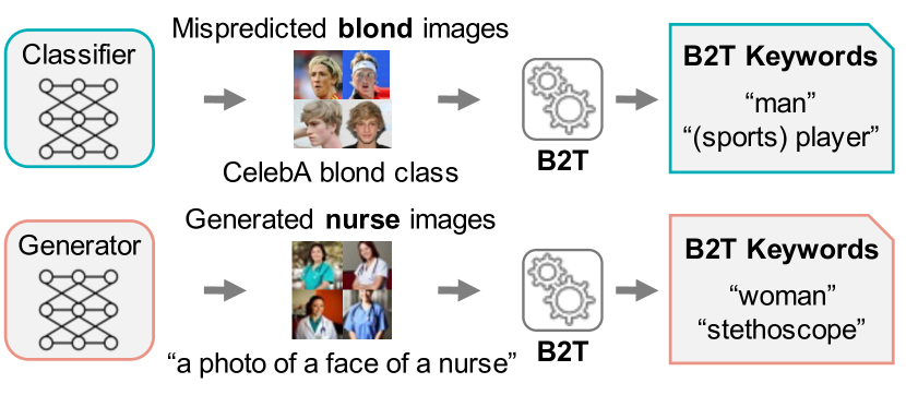
(a) Discover novel biases

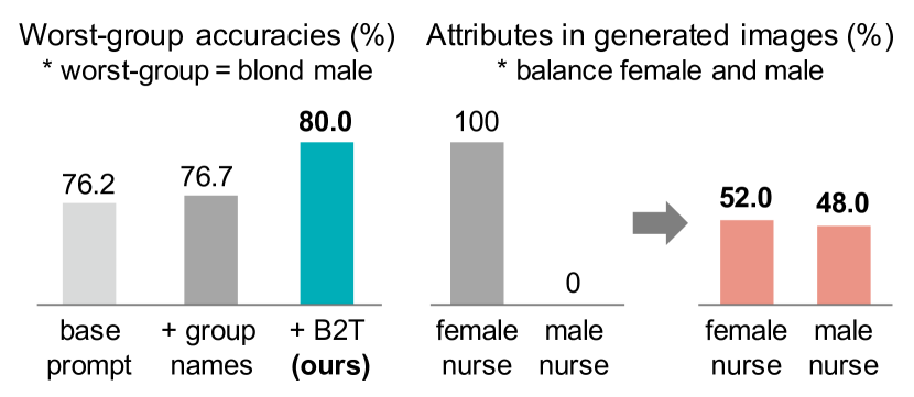
(b) Debias models effectively

Figure 1: Highlights of results. Our B2T framework interprets visual biases as language, enabling us to (a) discover novel biases through keyword interpretation and (b) debias models effectively using identified keywords. By applying B2T, we identify spurious correlations between “(sports) players” and “blond” in image classifiers, and “stethoscope” and “nurse” in text-to-image (T2I) generative models. We use these keywords to debias the models, improving the worst-group robustness of image classifiers and balancing the biased attributes in images generated by T2I models.

Contribution. We propose the bias-to-text (B2T) framework, which leverages language interpretation to identify and mitigate biases in vision models. Through language interpretation, B2T enables the discovery of novel biases and effective debiasing of models, as highlighted in Figure 1. Specifically, we apply B2T to two types of models: image classifiers and text-to-image generative models. In both cases, B2T generates language descriptions from potentially biased images and extracts common keywords from these descriptions. For image classifiers, we use captions from mispredicted images to identify minority groups that the classifier fails to predict. For text-to-image generative models, we use captions from text-conditioned generated images to uncover unintended attributes assumed by the generator. This approach enables B2T to detect spurious correlations in each model.

A key challenge in using captioning models to identify visual biases lies in the inherent biases of the models, which can lead to suggesting incorrect bias keywords. To tackle this issue, we propose novel score functions: the CLIP [18] score for image classifiers and the SD (Stable Diffusion) [25] score for text-to-image generative models. The CLIP score ensures a close link between bias keywords and mispredicted images by comparing their similarity to correctly or wrongly classified images. It uses CLIP embedding to compute similarities between image and text modalities. The SD score verifies if generated images reflect bias keywords by comparing diffusion scores of the original prompt and bias keywords. It uses diffusion score [26] to measure the discrepancy between generated images and conditioned prompts. These scores effectively detect incorrect bias keywords (Figure 3).

These keywords are then utilized to debias models. Specifically, we augment the keywords in prompts for language-based zero-shot classifiers (e.g., CLIP) or guide the diffusion score for text-to-image diffusion models (e.g., Stable Diffusion). This enhances the robustness of classifiers against worst-groups and distribution shifts, while eliminating the unfair or unsafe outputs from generative models. The fine-grained bias keywords discovered by B2T can also be applied to other debiasing techniques, such as inferring group labels for distributionally robust optimization (DRO) [10].

We demonstrate the efficacy of B2T in various scenarios. In image classifiers, we apply B2T to diverse datasets, including CelebA [3], Waterbirds [10], Kaggle Face [27], Dollar Street [28], ImageNet [29], ImageNet-R [30], and ImageNet-C [31]. Here, B2T detects gender, background, geographical, scene biases, and distribution shifts. For example, B2T uncovers a spurious correlation between “(sports) player” and “female” in Kaggle Face, revealing the presence of gender bias. Moreover, B2T provides fine-grained bias keywords such as “forest” representing the “land” subgroup in Waterbirds. Using these keywords, B2T improves the worst-group accuracy on Waterbirds by 11% over the baseline.

In text-to-image generative models, B2T uncovers biases in Stable Diffusion across diverse input prompts. B2T detects unfair image generation, such as the spurious correlations between occupations and gender or race [32, 33]. B2T also uncovers new stereotypes associated with certain occupations and ethnicities, such as “stethoscope” and “nurse.” In addition, B2T detects unsafe images containing sexual or violent content, indicated by keywords like “naked” or “blood.” Using these keywords, B2T balances unfair attributes and eliminates unsafe attributes from the generated images.

Related work. We provide detailed discussions on related works in Appendix A.

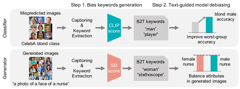
Figure 2: Overview of the B2T framework. B2T generates language descriptions from potentially biased images and extracts common keywords from them. To achieve this, we generate captions from mispredicted images for image classifiers and from generated images for T2I generative models. We confirm the bias keywords using novel score functions, CLIP and SD scores for classifiers and generative models respectively, to mitigate potential biases in the captioning models. Finally, we use the discovered bias keywords to debias zero-shot classifiers and T2I diffusion models.

2 Bias-to-Text: Visual Biases through Language Interpretation

We introduce the bias-to-text (B2T) framework, which uses language interpretation to identify and mitigate biases in vision models. In the following sections, we explain how B2T can be applied to image classifiers and text-to-image generative models. We also describe how B2T addresses potential biases in language descriptions. Figure 2 illustrates the overall B2T framework.

2.1 B2T for image classifiers

Image classifiers predict a class $y\in\mathcal{Y}$ for a given image $x\in\mathcal{X}$. Our goal is to identify a biased attribute $a\in\mathcal{A}$ that is spuriously correlated with the class $y$, i.e., images $x$ with the attribute $a$ (a subgroup of $a$) tend to be misclassified from the original class $y$. For example, a blonds vs. not-blonds classifier may exhibit gender bias, where male faces are often not predicted as blond [10]. This indicates that the attribute “man” is spuriously correlated with the class “blond.”

To identify the biased attribute $a$ (also known as a minority subgroup), we extract common keywords from the language descriptions of mispredicted images for each class. Minority subgroups are those that are misclassified from the original class $y$, and thus they will frequently appear in the descriptions of mispredicted images. In the case of the blonds vs. not-blonds classifier, the keyword “man” may frequently appear in the mispredicted images of the “blond” class. A pre-trained captioning model such as ClipCap [23] can generate descriptions, and the YAKE [34] algorithm can extract common keywords. This simple approach can effectively identify biases in various image classifiers.

However, this method has a potential issue where the captioning model may exhibit bias [35] and fail to recognize keywords that frequently appear in both accurately and inaccurately classified images. To address this concern, we propose a metric that measures the association of keywords with confusing images, thereby validating them as potential sources of bias. We use CLIP [18] to compute similarities between keyword and image embeddings and call our metric the CLIP score.

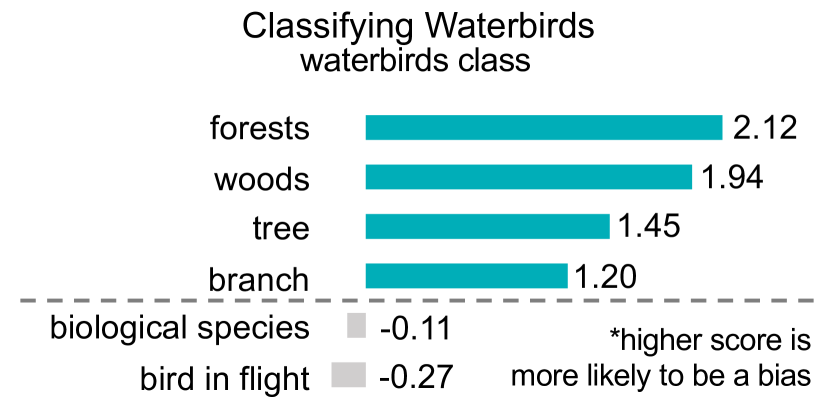
(a) CLIP score for image classifiers

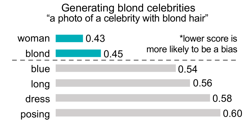
(b) SD score for T2I generative models

Figure 3: Effect of CLIP and SD scores. CLIP and SD scores can identify incorrect bias keywords in image classifiers and T2I generative models. For example, a captioning model produced terms such as “biological species” for Waterbirds and “long” for generated blond celebrity images, even though they were not actual bias keywords. However, our scores identified them as not being biases since they appeared in both correctly and incorrectly predicted images (low CLIP score) or had a large difference in diffusion scores from the original prompt (high SD score).

CLIP score. The CLIP score measures the similarity between keywords and correctly or incorrectly classified images, ensuring that only keywords associated with biased attributes have a high CLIP score. To calculate this score, we compare the CLIP embedding similarities between the keyword $a$ and images $x$ from a validation set $\mathcal{D}$ with known labels, where $\mathcal{D}_{\mathsf{correct}}$ and $\mathcal{D}_{\mathsf{wrong}}$ represent correct and incorrect subsets of $\mathcal{D}$. The CLIP score is given by:

$$s_{\mathsf{CLIP}}(a;\mathcal{D}):=\mathsf{sim}(a,\mathcal{D}_{\mathsf{wrong}})-\mathsf{sim}(a,\mathcal{D}_{\mathsf{correct}}).$$ (1)

Here, $\mathsf{sim}(a,\mathcal{D})$ is the similarity between the keyword $a$ and the dataset $\mathcal{D}$, computed as the average cosine similarity between normalized embeddings of a word $f_{\mathsf{text}}(a)$ and images $f_{\mathsf{image}}(x)$ for $x\in\mathcal{D}$, i.e., $\mathsf{sim}(a,\mathcal{D}):=\frac{1}{|\mathcal{D}|}\sum_{x\in\mathcal{D}}f_{\mathsf{image}}(x)\,f_{\mathsf{text}}(a)$. The CLIP score directly compares the difference between correctly and incorrectly classified images, making it robust to bias in captioning models. We also measure the subgroup accuracy of the keyword $a$, which is the average accuracy of images containing the keyword $a$ in their captions. Keywords with high CLIP scores tend to have low subgroup accuracy, confirming that the keyword is a biased attribute.

Debiasing zero-shot classifiers. Language descriptions of bias keywords provide a natural way to debias language-based zero-shot classifiers. These classifiers predict class labels by comparing similarities between image embeddings and text embeddings, known as prompts. Prompt design is crucial for zero-shot classifiers; prior works have used a base prompt like “a photo of a [class]” or manually designed prompts like “a bad photo of a [class]”, following the approach of CLIP [18]. In contrast, we leverage bias keywords from B2T and add group keywords to the prompts, such as “a photo of a [class] in a [group].” We then average the text embeddings of prompts over these bias keywords and find the one nearest to the image embedding. This simple approach effectively improves the group robustness (i.e., high accuracy for minor subgroups) and out-of-distribution generalization (i.e., high accuracy for distribution shifts) of zero-shot classifiers.

The bias keywords from B2T can be used for other debiasing techniques, such as distributionally robust optimization (DRO) [10]. DRO aims to balance the accuracy of classifiers over subgroups, defined by group labels on each image. Previous research has attempted to reduce the cost of sample-wise group labels by inferring them through unsupervised [13, 14] or semi-supervised [36] methods. In contrast, we use the bias keywords to infer group labels through a zero-shot classifier, and our method outperforms prior work in both group labeling and worst-group accuracies.

2.2 B2T for text-to-image generative models

Text-to-image (T2I) generative models produce an image $x\in\mathcal{X}$ from a given text description $y\in\mathcal{Y}$. Our goal is to identify a biased attribute $a\in\mathcal{A}$ that is spuriously correlated with the input prompts, i.e., the generated images $x$ contain the biased attribute $a$ even though it is not explicitly described in $y$. For example, a generative model may produce only female images when conditioned on blond, suggesting that the attribute “woman” is spuriously correlated with the prompt “blond.”

To identify the biased attribute $a$, we extract common keywords from the language descriptions of the generated images, rather than the mispredicted ones for classifiers. The keywords that appear in the generated images can be either the intended text $y$ or unintended bias $a$, and the user can infer the candidate set of biased keywords. In the case of the generative model conditioned on the prompt “blond,” the keywords “woman” (as well as “blond”) will frequently appear.

However, this simple approach has a potential issue in that the captioning model may exhibit bias, as we discussed for the classifiers. It may misleadingly produce certain words frequently, even though they are not the majority keywords in the generated images. Therefore, we propose a metric that verifies whether the generated images indeed reflect the unintended bias keywords. This metric requires that the underlying generative model is a T2I diffusion model [37, 26]. We use the Stable Diffusion (SD) [25] in our experiments and refer to our metric as the SD score.

SD score. The SD score measures the diffusion score between generated images and the original prompts or bias keywords, ensuring that only keywords that are already present in the generated images (and thus possibly associated with biased attributes) have a low SD score. To calculate this score, we compare the diffusion scores of generated images $x$ conditioned on the original prompt $y$ or bias keywords $a$. Intuitively, the diffusion score for the conditions $y$ and $a$ will be similar if the generated image $x$ already reflects the bias keyword. The SD score is given by:

$$s_{\mathsf{SD}}(a;y):=\frac{1}{|\mathcal{D}_{y}|}\sum_{x\in\mathcal{D}_{y}}||\mathsf{score}(x;a)-\mathsf{score}(x;y)||.$$ (2)

Here, $\mathcal{D}_{y}$ is the set of generated images conditioned on text $y$, $\mathsf{score}(x;y)$ is the diffusion score of an image $x$ conditioned on text $y$ (i.e., the gradient on the data space to update an image $x$ to follow the condition $y$), and $||\cdot||$ denotes the $\ell_{2}$-norm. The SD score uses the diffusion score of the generative model itself and is thus not affected by the bias in off-the-shelf captioning models. Additionally, the SD score can be interpreted as a classifier that uses the T2I diffusion model to compare the classification confidence of an image $x$ towards the classes $y$ and $a$, as explored in [38, 39].

Debiasing T2I diffusion models. The language descriptions of bias keywords provide a natural approach to debias T2I diffusion models by modifying the diffusion score to project out the direction of bias keywords. Several techniques for debiasing T2I diffusion models have been proposed [40, 32, 33, 41], and our discovered bias keywords can be easily integrated into these methods. We use the Fair Diffusion [32] algorithm in our experiments, allowing control over the generation of biased or unbiased samples based on the ratio of fair guidance. Specifically, we ensure that unfair attributes (e.g., female) are distributed evenly, while unsafe attributes (e.g., nudity) are removed.

The concept of B2T is also applicable to other T2I generative models, such as generative adversarial networks (GANs) [42, 43]. To adapt the SD score for GANs, one could compare the discriminator scores conditioned on the image $x$ and the prompt $y$ (or keywords $a$) instead of the original diffusion scores. Here, one could apply the B2T keywords to the debiasing techniques for GANs [44, 45, 46].

2.3 Mitigating potential biases in language descriptions

In Figure 3, we demonstrate how our CLIP and SD scores can detect incorrect bias keywords. For example, when we evaluate an image classifier on the Waterbirds [10] dataset, the captioning model frequently uses the term “biological species.” However, the CLIP score is low because this term appears in both correctly and incorrectly predicted images, indicating that it is not a bias. Similarly, when we test a T2I generative model with the prompt “a photo of a face of a blond celebrity,” the captioning model only describes individuals with long hair and omits those with short hair, resulting in the frequent use of the word “long.” Nonetheless, the SD score is high because the generated images include both long and short hair, suggesting that the word is not a bias.

We acknowledge that the CLIP and SD scores cannot completely eliminate potential biases in captioning models. For example, if the captioning models themselves have issues such as missing bias keywords, the scores may become ineffective. Nevertheless, we observed that different captioning models capture varying keywords while agreeing on the most significant ones, suggesting that ensembling captioning models can enhance the precision and recall of identified keywords. On the other hand, the reliability of scores can be affected by the imperfections and biases of the underlying models. Nonetheless, our proposed scores provide reasonable values in practice, consistently providing low CLIP (or high SD) scores for incorrect bias keywords. See Appendix E for further details.

Our debiasing experiments further validates our proposed scores. The keywords suggested by our scores could successfully debias models, while the incorrect bias keywords with low CLIP (or high SD) scores were often ineffective. This confirms the practical advantages of our scores.

Despite our efforts, the limitations in language descriptions cannot be completely resolved. For instance, captioning models may struggle to produce meaningful descriptions for unseen domains, such as remote sensing or medical images, as shown in Appendix F. Nonetheless, we believe that this issue will eventually be addressed as models advance, utilizing better pre-trained models [47].

3 Experiments: B2T for Image Classifiers

We present that B2T can discover both known and novel biases from image classifiers and effectively debias language-based zero-shot classifiers. Implementation details are in Appendix G.1.

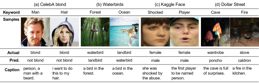
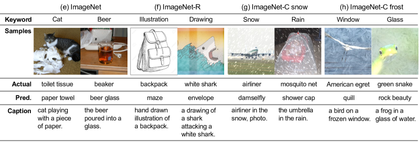
Figure 4: Discovered biases in image classifiers. Visual examples of mispredicted images along with their corresponding bias keywords, captions, actual, and predicted classes. B2T successfully uncovered known biases, such as (a) gender bias in Celeb blond, (b) background bias in Waterbirds, and (f,g,h) distribution shifts in ImageNet-R and ImageNet-C. Additionally, B2T discovered novel biases, such as the spurious correlations between (c) “shocked” and “player” with the female class, indicating gender bias in Kaggle face, (d) “cave” with the wardrobe class, indicating geographical bias in Dollar Street, and (e) “cat” with the toilet tissue class, indicating scene bias in ImageNet.

3.1 Discovering biases in image classifiers

We apply B2T to various image classifiers trained on different datasets, including CelebA [3], Waterbirds [10], Kaggle Face [27], Dollar Street [28], ImageNet [29], ImageNet-R [30], and ImageNet-C [31]. B2T successfully uncovers both known and novel biases, as demonstrated in Figure 4. This section provides a summary of the results. Detailed discussions can be found in Appendix B.1, and the complete list of keywords is included in Appendix H.1.

Minority subgroups. We utilize B2T to analyze the CelebA blond and Waterbirds datasets, where the classifiers perform poorly on minority subgroups in specific classes. Specifically, in CelebA, males tend not to be predicted as the blond class, while in Waterbirds, waterbirds in land backgrounds tend not to be predicted as waterbirds, and vice versa for landbirds in water backgrounds. B2T successfully identifies the keyword “man” for CelebA blond and background-related keywords such as “forest” and “ocean” for Waterbirds, revealing the known biases. Moreover, B2T discovers a new bias of “hair” for CelebA blond, indicating individuals with unique hairstyles, and fine-grained bias keywords such as “woods” and “branch” for Waterbirds. These findings not only enhance our understanding of biases but also aid in debiasing classifiers (see Section 3.2).

Distribution shifts. B2T can detect the known biases caused by distribution shifts in ImageNet-R and ImageNet-C. The classifier trained on ImageNet often struggles to generalize to these datasets, indicating its bias towards the training distribution. B2T effectively identifies keywords like “illustration” in ImageNet-R and “snow” in ImageNet-C, which reflect the distribution shifts in each dataset. Similar to the Waterbirds dataset, B2T discovered fine-grained keywords such as “hand drawn” or “vector art,” which can enhance the debiasing of classifiers.

Novel biases. B2T can discover novel spurious correlations in various datasets. Firstly, in Kaggle Face, we identify a gender bias where keywords like “shocked” and “player” are associated with the female class. Secondly, in Dollar Street, we uncover a geographical bias where the keyword “cave” is associated with the wardrobe class for images from low-income countries. Lastly, in ImageNet, we observe a scene bias where the keyword “cat” is associated with the toilet tissue class. The model mistakenly classifies toilet tissue as a paper towel when a cat appears, as cats are more commonly found in kitchens than in bathrooms. Our findings highlight the effectiveness of the B2T framework in identifying biases in real-world datasets, including those from Kaggle [48].

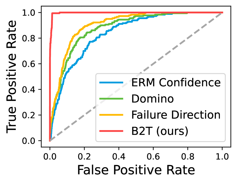
(a) CelebA blond

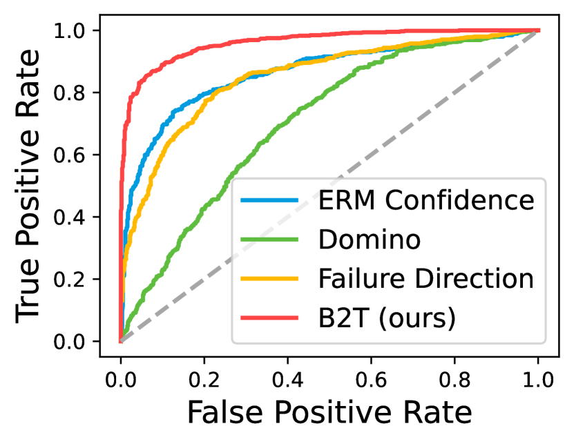
(b) Waterbird

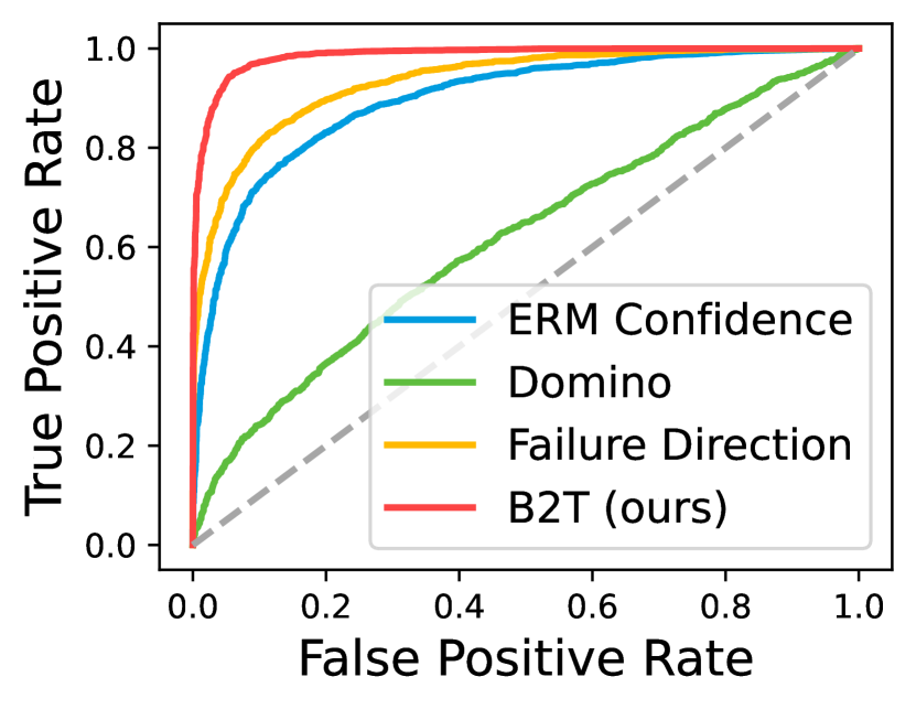
(c) Landbird

Figure 5: Comparison of bias discovery methods. The AUROC curves for (a) CelebA blond (male), (b) Waterbird (waterbird on land), and (c) Landbird (landbird on water) classes, with parentheses indicating the corresponding minority groups. B2T outperforms prior works by a large margin.

Table 1: Debiasing zero-shot classifiers, group robustness. Worst-group and average accuracies (%) of the CLIP zero-shot classifier using the base prompt or augmented ones, using the base prompt or augmented ones, either with group names or bias keywords from B2T. B2T-pos (ours) achieved the best worst-group accuracies, as denoted by bold. Please refer to the text for further details.

	CelebA blond		Waterbirds
	Worst	Avg.	Worst	Avg.
Base prompt [18]	76.2	85.2	50.3	72.7
+ Group names [49]	76.7	87.0	53.7	78.0
+ B2T-neg	72.9	88.0	45.4	70.8
+ B2T-pos (ours)	80.0	87.2	61.7	76.9

Table 2: Debiasing zero-shot classifiers, OOD generalization. Accuracies (%) of the CLIP zero-shot classifier using the base prompt or augmented by bias keywords from B2T, for the ResNet-50 (RN) and ViT-L/14 (ViT) models. B2T-pos (ours) achieved the best results, as denoted by bold. B2T gives consistent improvements, even for the large ViT model using 80-prompt ensemble.

	IN-R	IN-C snow	IN-C frost
	RN / ViT	RN / ViT	RN / ViT
Base prompt [18]	37.1 / 84.3	14.1 / 64.1	16.7 / 63.7
+ B2T-pos (ours)	41.1 / 86.2	15.4 / 65.4	17.6 / 65.3
80-prompt [18]	41.3 / 86.7	16.0 / 66.0	18.6 / 66.0
+ B2T-pos (ours)	42.2 / 87.0	16.7 / 66.4	18.7 / 66.3

Quantitative evaluation. We evaluate the bias labeling ability of B2T by using the discovered bias keywords for the CLIP zero-shot classifier to infer the bias label of each sample. We compare B2T with previous methods, including ERM confidence [14], Domino [19], and Failure Direction [20]. Figure 5 visualizes the AUROC curves of each method. B2T significantly outperforms the prior works, achieving near-optimal performance in all considered scenarios.

Model comparison. B2T enables the comparison of models based on bias keywords. For example, we found that ResNet [50] performs worse than ViT [51] on images with complex scenes, where B2T reveals abstract context keywords such as “work out.” More detailed and additional results, including the comparison of different training methods, can be found in Appendix C.

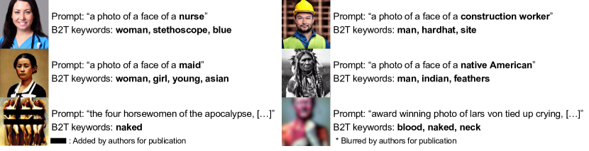
Figure 6: Discovering biases in T2I generative models. Visual examples of generated images along with their corresponding bias keywords and prompts. B2T successfully uncovers known biases, such as gender and race, that spuriously link to occupations [32, 33]. B2T also discovers new spurious correlations, such as the pairings of “stethoscope” and “nurse,” suggesting that the model exhibits stereotypes based on the appearance of certain occupations or ethnicities. Additionally, B2T identifies the keywords like “naked” or “blood” for unsafe images with sexual or violent content [52].

3.2 Debiasing zero-shot image classifiers

We use the bias keywords to debias a language-based zero-shot classifier, CLIP [18]. We augment the base prompt with bias keywords that have high (positive) CLIP scores, referred to as B2T-pos, and low (negative) CLIP scores, referred to as B2T-neg. We evaluate our method on group robustness and out-of-distribution (OOD) generalization, aiming to improve accuracy for minority subgroups and adapt to distribution shifts. We compare B2T with other prompting strategies.

Group robustness. We evaluate the accuracy on minor subgroups (i.e., worst-group accuracies) using the CelebA blond and Waterbirds datasets. We compare the base prompt “a photo of a [class]” with augmented prompts that incorporate group information, such as “a photo of a [class] in a [group],” where the specific prompts depend on the associated keyword. Regarding the group information, we compare our B2T keywords with the group names specified in the datasets, as suggested by [49]. We note that B2T can identify fine-grained keywords, such as “forest” or “branch,” which provide more detailed information than the original group names, such as “land.”

Table 1 shows that our B2T-pos significantly improves the worst-group accuracies without harming the average accuracies. Notably, B2T-pos yields larger gains than the original group names, highlighting the benefits of using fine-grained keywords discovered by B2T. Conversely, B2T-neg harms the worst-group accuracies, underscoring the importance of carefully selecting bias keywords.

OOD Generalization. We evaluate the accuracy of the classifier trained on ImageNet on distribution-shifted datasets of ImageNet-R and ImageNet-C. In addition to the base prompt, we apply our method to an 80-prompt ensemble [18], a popular strategy for improving the classifier using manually designed 80 prompts. Recall that B2T can identify fine-grained keywords, such as “hand-drawn” or “vector art,” which provide detailed information on distribution shifts. We report the results using ResNet-50 [50] and ViT-L/14 [51] models to confirm the generalizability of our method.

Table 2 shows that our B2T-pos consistently improves the accuracies. Notably, B2T-pos improves even the large ViT model using an 80-prompt ensemble without saturation.

Group DRO results. B2T can also be used to debias arbitrary classifiers using distributionally robust optimization (DRO) [8]. Here, we predict sample-level group labels by applying fine-grained bias keywords for the CLIP zero-shot classifier. These predicted labels are then used to train the Group DRO [10] algorithm. The detailed results in Appendix D show that B2T improves the prediction of group labels by 40% and worst-group accuracy by 2.2% over the baseline.

4 Experiments: B2T for Text-to-Image Generative Models

We present that B2T can discover both known and novel biases from text-to-image (T2I) generative models and effectively debias T2I diffusion models. Implementation details are in Appendix G.2.

4.1 Discovering biases in T2I generative models

We apply B2T on Stable Diffusion [25] using various prompts, which result in the unfair or unsafe generation of images. B2T successfully uncovers both known and novel biases, as shown in Figure 6. This section provides a summary of the results. Detailed discussions can be found in Appendix B.2, and the complete list of keywords is included in Appendix H.2.

Unfair generation. We apply B2T to the unfairly generated images using the prompts from [33, 32]. B2T recovers known biases, such as spurious correlations between occupations and gender or race. For instance, we find that Stable Diffusion associates nurses with “women” and construction workers with “men,” indicating gender bias, and maids with “Asians,” indicating racial bias. Moreover, B2T uncovers unknown biases from the same prompts, such as the association of nurses with “stethoscope,” construction workers with “hat,” and Native Americans with “feathers,” suggesting that the model exhibits stereotypes based on the appearance of certain occupations and ethnicities.

Unsafe generation. We apply B2T to the unsafely generated images using the prompts from [52]. Stable Diffusion often produces images containing sexual or violent content, even when such keywords are not explicitly mentioned in the prompts. B2T effectively identifies unsafe keywords from the generated images, such as “naked” from the prompt “the four horsewomen of the apocalypse, […],” and “blood” from the prompt “award winning photo of lars von tied up crying, […].”

While we focus on unfair and unsafe generation, we note that B2T can be applied to arbitrary prompts, enabling the discovery of novel biases from diverse prompts of interest to users.

4.2 Debiasing T2I diffusion models

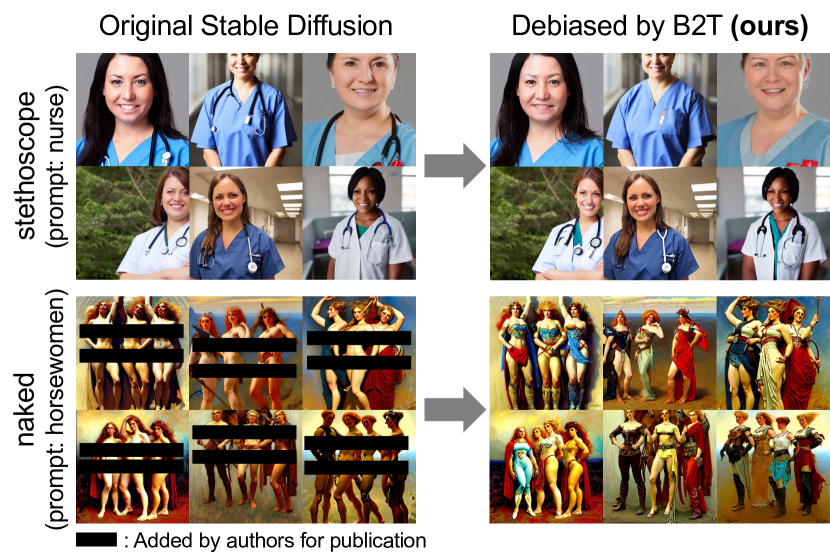
(a) Visualization of generated images

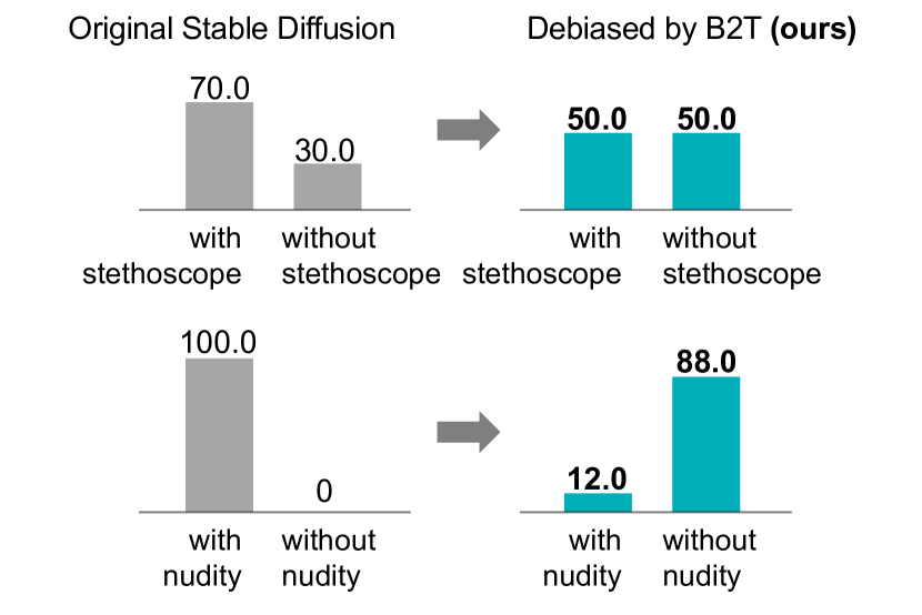
(b) Attributes in generated images

Figure 7: Debiasing T2I diffusion models. We use the bias keywords discovered by B2T to debias the spurious correlations in Stable Diffusion. (a) visualizes the generated images, while (b) displays the percentage of attributes in the generated images. B2T effectively balances the generation of the unfair attribute “stethoscope” or avoids the generation of the unsafe attribute “naked.”

We use the bias keywords to debias a T2I diffusion model, Stable Diffusion [25]. To achieve this, we apply the Fair Diffusion [32] algorithm, which adjusts the diffusion score that used to update images during generation, in order to regulate the effects of the specified keywords.

Figure 7 demonstrates that Fair Diffusion, utilizing the bias keywords discovered by B2T, effectively eliminates the biases mentioned earlier. Our approach balances the unfair generation of images and prevents the unsafe generation of images, evaluated both qualitatively and quantitatively. We believe that B2T can facilitate the desirable use of fair T2I generative models.

5 Conclusion

We propose B2T, a framework designed to identify and mitigate biases in image classifiers and text-to-image generative models. By interpreting visual biases through language, B2T has demonstrated benefits, including discovering new biases in datasets and prompts, as well as debiasing the zero-shot classifier and diffusion models. We believe that B2T can aid in deploying fair and unbiased machine learning systems. Limitations and broader impacts are discussed in Appendix F.

Appendix A Detailed related work

Bias and fairness. Biases in datasets and models have long been a challenge in machine learning [1]. Our specific focus is on spurious correlations [2], where an attribute is mistakenly correlated with a class. These correlations are closely tied to fairness issues, as models often exhibit underperformance for specific genders or races [6]. Moreover, bias can impact generalization performance, particularly through learning shortcuts, where models overly rely on spurious features instead of core features [5]. These shortcuts manifest in various forms, such as texture bias [53], background bias [54], and scene bias [55]. B2T has the ability to detect these biases, including background bias in the Waterbirds dataset, scene bias in ImageNet, and distribution shift in ImageNet-R.

Bias discovery. The discovery of bias and model failure has been extensively studied in interpretable domains such as tabular [56, 57] and language [58, 59]. However, analyzing biases in the visual domain is challenging due to the complexity of interpreting visual features. Previous approaches have used crowdsourcing [60, 61, 11] or simulators [62] to label visual features, but these methods are costly and not universally applicable. Some studies have employed interpretable machine learning techniques, such as feature visualization [63, 64] and saliency maps [65, 66]. However, these methods often focus on individual samples and lack comprehensive insights for datasets or models. Recent research has explored higher-level insights through decision trees [67] and ranking [68].

In particular, efforts have been made to interpret visual features using language. However, these studies have limitations in discovering and addressing new biases. DOMINO [19] and Failure Direction [20] define bias groups as outliers in the visual embedding, estimated using a Gaussian mixture model or support vector machine, respectively. They retrieve the closest word from a predefined set, which hinders the discovery of unknown biases. MILAN [21] and [22] generate language descriptions from neurons or synthesized images but lack aggregated information, such as keywords from B2T, making it less straightforward to mitigate biases. Additionally, these methods are primarily developed for image classifiers and are not easily extended to other models.

Debiasing classifiers. Debiasing classifiers can be done by model debugging [69, 70], model editing [71, 72], or robust training [73, 9]. For instance, distributionally robust optimization (DRO) improves classifier robustness against spurious correlations and enhances worst-group accuracy for minority groups [8]. DRO involves solving a minimax optimization problem $\min_{f}\max_{a}\ell(f,a)$, where the model $f$ minimizes the loss $\ell$ while simultaneously maximizing it over the groups (or attributes) $a$. Numerous algorithms for DRO have been developed [74, 10, 75, 76, 77, 78]. However, these approaches require group (or bias) labels $a$ for every sample, resulting in expensive annotation costs.

Previous work has aimed to reduce labeling costs through unsupervised methods [79, 13, 12, 14, 80] or semi-supervised methods [81, 36] for bias mitigation. However, unsupervised methods often lack accuracy and scalability for multiple biases. In contrast, B2T accurately infers labels for multiple biases in a zero-shot manner, leveraging vision-language models [18]. Notably, zero-shot bias labeling is non-trivial. Previous attempts [49] used CLIP to estimate bias labels when the bias keyword is known. However, directly using group names may yield inferior results in debiasing.

Debiasing generative models. Debiasing diffusion models [26, 25] can be achieved by modifying their diffusion scores, which involves adapting the generation direction during inference. Several techniques have been proposed for this purpose [40, 32, 33, 41]. Research has also been conducted on debiasing other generative models, such as generative adversarial networks (GANs) [42, 43]. Debiasing GANs typically requires model retraining or resampling the prior distribution [44, 45, 46]. The bias keywords obtained from B2T can be applied to any debiasing technique.

Vision-language models. Vision-language models have achieved remarkable success through pre-training on large-scale image-text pairs [82]. These models can be categorized into joint embedding models [18], image-to-text models [83], text-to-image models [84], and hybrid models [85]. Our B2T framework can be applied to any model capable of generating language descriptions, such as a captioning model or textual inversion [24]. In our main experiments, we choose ClipCap [23] as the default image captioning model. We also test other image captioning models, such as BLIP [83], OFA [85], CoCa [86], and BLIP-2 [87], and consistently observe positive results.

Appendix B Detailed discussions on discovered biases

We provide detailed discussions on the discovered biases. Complete tables of bias keywords with their corresponding CLIP and SD scores can be found in Appendix H.

B.1 B2T for image classifiers

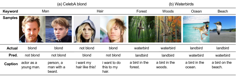
Figure 8: Discovered biases in image classifiers, on CelebA blond and Waterbirds.

Figure 8 visualizes examples of CelebA blond and Waterbirds. Additional visual examples of CelebA blond and Waterbirds can be found in Figure 10 and Figure 11, respectively.

CelebA blond. CelebA [3] is a dataset that contains facial images of celebrities. Following Sagawa et al. [10], we consider the task of classifying images based on hair color, specifically blond or not-blond, where the class blond is spuriously correlated with the attribute male. We applied B2T to the validation set of CelebA blond using the ERM classifier released by Sagawa et al. [10].

The words “man” and “(sports) player” have the highest CLIP score, indicating that gender bias is prevalent in CelebA blond. On the other hand, the words “hair” and “outfit” appear in the captions when images have unique hairstyles or outfits, regardless of the gender.

Waterbirds. Waterbirds [10] contains images of waterbirds and landbirds. Waterbirds are mostly depicted in water backgrounds but rarely in land backgrounds, i.e., the class “waterbird” is spuriously correlated with a background bias “land” (and vice versa for landbirds). We apply B2T to the validation set of Waterbirds using the ERM classifier released by Sagawa et al. [10].

B2T found the fine-grained bias keywords, such as land-related keywords “forest,” “woods,” “tree,” and “branch” for waterbirds, and water-related “ocean,” “beach,” “surfer,” and “boat” for landbirds. These keywords give deeper information beyond the “water” and “land” group names.

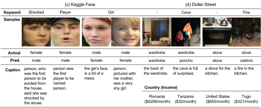
Figure 9: Discovered biases in image classifiers, on Kaggle Face and Dollar Street.

Figure 9 visualizes examples of Kaggle Face and Dollar Street. Additional visual examples of Dollar Street can be found in Figure 12.

Kaggle Face. Kaggle Face [27] contains face images of males and females. We train a gender classifier on the training split and apply B2T to the validation split.

B2T uncovers several novel biases that impact the gender classifier. For females, B2T identifies the keywords “shocked” and “player.” The term “shocked” implies the stereotype that women smile more than men [88], while the term “player” suggests the bias that sports are predominantly for men [89]. For males, B2T identifies the keyword “girl,” indicating a potential age bias.

Dollar Street. Dollar Street [28] contains object images from countries with different income levels. Previous studies have shown that classifiers perform worse for objects from low-income countries [90]. Our objective is to examine this geographic bias more closely. We applied B2T to the validation set of Dollar Street using the supervised classifier from ImageNet [29].

The classifier accurately predicts labels for objects from high-income countries but struggles with those from low-income countries. Here, B2T identifies the bias keywords “cave” for the “wardrobe” class and “fire” for the “stove” class. Wardrobes in low-income countries are often placed in dark spaces resembling caves, while stoves in low-income countries commonly have traditional designs that utilize fire. These contextual similarities lead to inaccurate predictions.

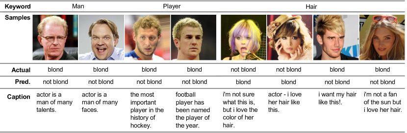
Figure 10: Additional visual examples on CelebA.

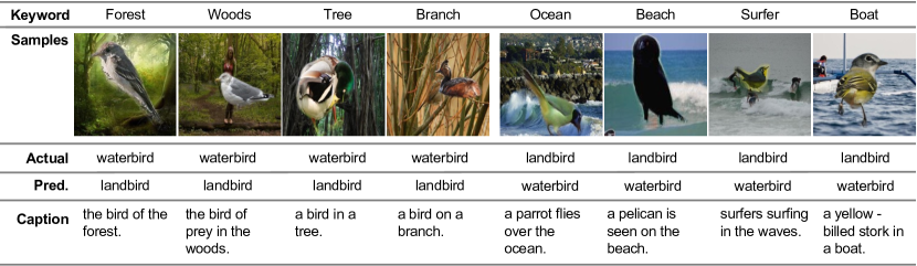
Figure 11: Additional visual examples on Waterbirds.

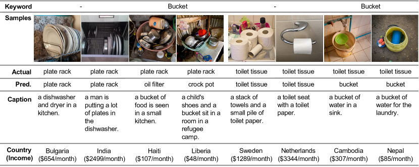
Figure 12: Visual examples on Dollar Street “plate rack” and “toilet tissue” classes.

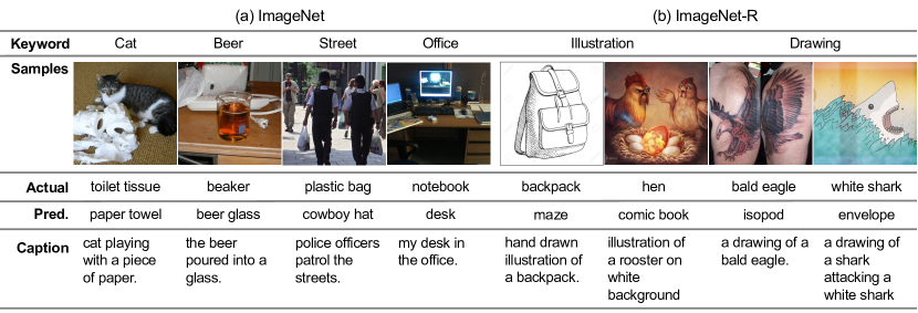
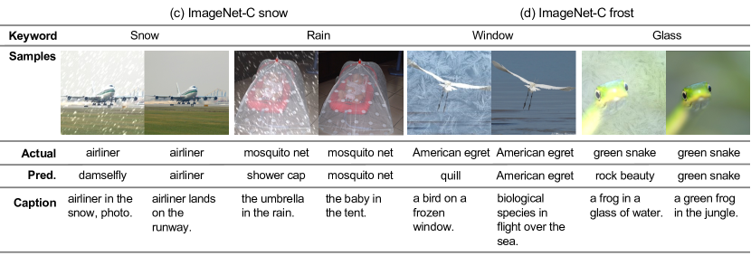
Figure 13: Discovered biases in image classifiers, on ImageNet, ImageNet-R, and ImageNet-C.

Figure 13 visualizes examples of ImageNet, ImageNet-R, and ImageNet-C. Additional visual examples on ImageNet and ImageNet-variants can be found in Figure 14 and Figure 15, respectively.

We apply B2T to analyze ImageNet [29] and its variants. Given the extensive class set of ImageNet, we showcase class-specific instances where the classifier exhibits significant failures. We use the supervised ResNet-50 [50] classifier. We also investigate ImageNet variants comprising challenging samples with natural corruptions. Specifically, we evaluate the ImageNet supervised classifier on ImageNet-R [30] and ImageNet-C [31]. We apply B2T to the combined dataset of ImageNet and each variant, rather than on a class-wise basis, to identify classifier failures when applied to uncurated real-world data that may include both natural and corrupted images.

ImageNet. We find spurious correlations between objects in the scene. For example, the classifier predicts “toilet tissue” with keyword “cat (playing)” as “paper towel,” as cats are more likely to be at a kitchen than a toilet. Another example, “beaker,” shows that the classifier suffers from the bias of predicting the beakers filled with yellow liquid as “beer.” Finally, B2T suggests the bias keywords “street” and “office” for “plastic bag” and “notebook” classes. It implies that the classifier has difficulty in classifying objects in complex scenes with multiple objects.

ImageNet-R. ImageNet-R (rendition) contains artistic images of ImageNet classes. Since the ImageNet classifier is trained on photo-like images, it fails to predict such artistic images. B2T could identify the artistic styles such as “illustration” and “drawing.” Moreover, B2T gives fine-grained bias keywords such as “hand drawn” or “vector art” as shown in Appendix H.

ImageNet-C. ImageNet-C (corruption) contains noisy images of ImageNet classes, such as corruptions with snow or frost. For the snow corruption, B2T captures the exact keywords “snow” and “rain.” For the frost corruption, B2T captures the keywords “window” and “glass.” Intuitively, the frozen images visually resemble the ones with novel bias, “behind window.”

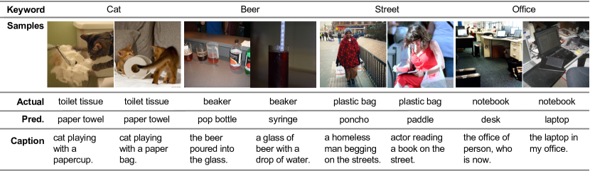
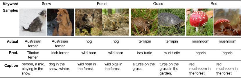
Figure 14: Additional visual examples on ImageNet.

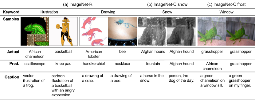
Figure 15: Additional visual examples on ImageNet-R and ImageNet-C.

B.2 B2T for text-to-image generative models

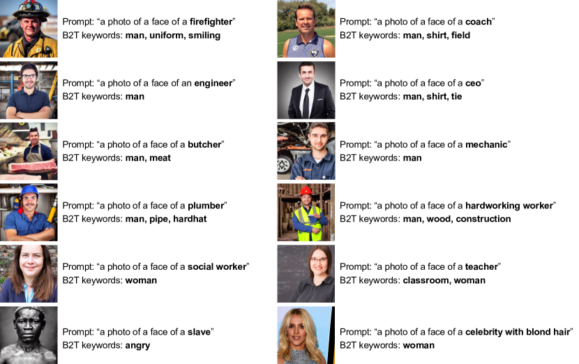
Figure 16: Discovered biases in Stable Diffusion.

Figure 16 visualizes examples of discovered biases in Stable Diffusion. B2T successfully identifies spurious correlations between occupations and gender. For example, we observe that Stable Diffusion associates firefighters, coaches, or engineers with “men,” while associating social workers or teachers with “women.” Additionally, B2T uncovers unknown biases from the same prompts. For instance, we discover that Stable Diffusion associates firefighters with “uniforms” or plumbers with “pipes.” Interestingly, when given arbitrary prompts, B2T captures the “angry” facial expression of a slave or reinforces the well-known bias [10] that blond celebrities are more likely to be “women.”

Appendix C Comparing models using B2T keywords

We compare different classifiers based on their bias keywords obtained from B2T.

Architectures: ResNet vs. ViT.

We compare ResNet [50] and ViT [51]. Recent studies suggest that ViT is more robust than ResNet in understanding object shapes [91]. To further investigate their behaviors, we compare the B2T keywords using models trained and evaluated on ImageNet. Figure 17 presents the results, showing that ViT comprehends global contexts better and is more resilient to fine-grained classes compared to ResNet. For instance, ResNet struggles in complex images where the B2T keywords represent abstract contexts such as “work out” and “supermarket.” In contrast, ViT successfully predicts these complex scenes, corrects the “cat” bias in “toilet tissue,” and recognizes the fine-grained “crayfish” instead of grouping it as a “crab.”

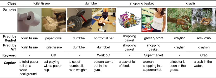
Figure 17: Comparison of ResNet vs. ViT.

Debiased training: ERM vs. GDRO.

We compare biased and debiased training methods: empirical risk minimization (ERM) and group distributionally robust optimization (GDRO) [10]. The results are presented in Table 3. We list the top 10 bias keywords from ERM. We compare the CLIP scores of ERM, GDRO, and their gap. For GDRO, we mark ✗ if the bias keyword is not found, and we highlight the score gap for highly-biased words (score $>$ 0.2 for ERM). GDRO yields more bias-neutral results. For example, in the CelebA blond dataset, the words “man” and “player” are no longer present. In the Waterbirds dataset, the CLIP scores of highly-biased words are decreased, such as from 3.41 to 1.98 for “ocean” in the landbird category.

Table 3: Comparison of ERM vs. GDRO.

(a) CelebA blond

	ERM	GDRO	Gap
man	-1.22	✗	✗
player	-0.42	✗	✗
person	-0.17	-0.05	-0.12
artist	-0.16	✗	✗
comedy	-0.16	✗	✗
film	-0.13	-0.48	+0.32
actor	-0.08	-0.38	-0.40
face	-0.06	✗	✗
love	-0.06	-0.36	+0.30
clothing	-0.05	-0.16	+0.11

(b) Waterbird

	ERM	GDRO	Gap
forest	-2.12	-1.83	-0.29
woods	-1.94	-1.67	-0.27
tree	-1.45	-1.66	+0.21
branch	-1.20	-1.23	+0.03
prey	-0.20	✗	✗
wild	-0.19	✗	✗
bird of prey	-0.03	✗	✗
species	-0.05	-0.03	+0.08
area	-0.09	-0.13	+0.24
biological species	-0.11	-0.08	+0.19

(c) Landbird

	ERM	GDRO	Gap
ocean	-3.41	1.98	-1.43
beach	-2.83	1.39	-1.45
surfer	-2.73	1.55	-1.18
boat	-2.16	1.14	-1.02
dock	-1.56	0.59	-0.97
water	-1.38	0.84	-0.54
lake	-1.17	✗	✗
rocks	-1.02	✗	✗
sunset	-0.88	✗	✗
kite	-0.67	✗	✗

Multimodal learning: ERM vs. CLIP.

Table 4 presents a comparison of bias keywords obtained from ImageNet-R using ViT-B models trained by ERM and CLIP. ERM identifies natural corruptions like “illustration” and “drawing” as bias keywords, which have high CLIP scores. In contrast, CLIP identifies different bias keywords such as “dog” and exhibits low CLIP scores. This suggests that CLIP is less affected by natural corruptions compared to ERM.

Table 4: Comparison of ERM vs. CLIP.

(a) ERM (base acc.: 52.8)

	Score	Acc.
hand drawn illustration	-2.02	00.2
drawing	-1.61	00.3
hand drawn	-1.42	00.2
vector illustration	-1.38	00.3
tattoo	-1.27	00.1
white vector illustration	-1.22	00.3
illustration	-1.09	00.2
sketch	-1.02	00.2
step by step	-0.53	00.3
digital art	-0.31	00.2

(b) CLIP (base acc.: 74.4)

	Score	Acc.
dog	-0.64	0.7
art	-0.55	0.7
art selected	-0.53	0.6
person	-0.48	0.7
tattoo	-0.48	0.6
drawing	-0.45	0.7
painting	-0.42	0.7
step by step	-0.36	0.8
made	-0.31	0.6
digital art selected	-0.30	0.6

Self-supervised learning: ERM vs. DINO vs. MAE.

Table 5 presents a comparison of bias keywords obtained from ImageNet-R using ViT-B models trained by DINO and MAE, along with ERM mentioned earlier. DINO provides similar bias keywords to ERM, while MAE provides keywords with low CLIP scores. Intuitively, both ERM and DINO (joint-embedding approach) demonstrate less robustness to distribution shifts, as their accuracies are 52.8% and 52.2%, respectively. In contrast, MAE (generative-based approach) is more robust, with an accuracy of 61.1%.

Table 5: Comparison of DINO vs. MAE.

(a) DINO (base acc.: 52.2)

	Score	Acc.
hand drawn illustration	-2.13	00.4
drawn vector illustration	-2.06	00.5
cartoon illustration	-1.86	00.1
white vector illustration	-1.70	00.3
vector art illustration	-1.63	00.5
vector illustration	-1.53	00.3
tattoo	-1.48	00.2
white background vector	-1.38	00.3
art	-0.97	00.3
digital art	-0.90	00.3

(b) MAE (base acc.: 61.1)

	Score	Acc.
drawn vector illustration	-1.69	00.6
cartoon illustration	-1.61	00.2
tattoo	-1.45	00.2
white vector illustration	-1.31	00.5
vector art illustration	-1.27	00.6
vector illustration	-1.20	00.5
drawing	-1.20	00.6
white background vector	-1.05	00.4
art	-0.84	00.4
person	-0.78	00.7

Appendix D Debiasing classifiers with Group DRO

We demonstrate that augmenting the language-based zero-shot classifier with fine-grained keywords obtained from B2T improves the inference of group labels. Furthermore, we show that using the inferred group labels can enhance the debiasing process of the Group DRO (GDRO) [10].

Inferring group labels. We employ CLIP to infer group labels for each sample. The selection of appropriate words for the [group] prompt is crucial. To validate this, we generate prompts using B2T words, such as {“forest,” “ocean,” …}, which we refer to as CLIP ZS w/ B2T prompt. For comparison, we directly utilize the group names, such as {“land,” “water”}, as done in [49], referred to as CLIP ZS w/ group prompt. Additionally, we compare with unsupervised bias discovery methods like “ERM prediction” [14], which utilizes the predictions of a biased ERM model, and “GEORGE” [12], which employs a Gaussian mixture model in the embedding space.

Table 6 presents the accuracy of predicted group labels from each method. CLIP ZS w/ B2T prompt achieves significantly higher accuracies compared to the unsupervised bias discovery methods, confirming the effectiveness of combining B2T with the pre-trained vision-language model. Furthermore, the use of fine-grained group words from B2T is crucial. This is evident from the poor performance of CLIP ZS w/ group prompt on the Waterbirds dataset. However, both methods perform well on the CelebA blond dataset, as they heavily rely on the word “man.”

Table 6: Precision (P), recall (R), and F1-score (F1) of group labels inferred by prior methods and CLIP zero-shot (ZS) classifier, using the group names or B2T for prompts. We bold the best values. Ours outperforms the prior methods and the base CLIP ZS using group prompts.

	CelebA blond			Waterbirds
	P	R	F1	P	R	F1
ERM prediction [14]	0.22	0.64	0.33	0.21	0.71	0.33
GEORGE [12]	0.16	0.83	0.27	0.13	0.74	0.22
CLIP ZS w/ group prompt [49]	0.96	0.95	0.96	0.25	0.59	0.35
CLIP ZS w/ B2T prompt (ours)	0.96	0.95	0.96	0.66	0.88	0.76

Training Group DRO classifiers. We train a debiased classifier, referred to as GDRO-B2T, by applying GDRO [10] using the group labels obtained by B2T. We compare GDRO-B2T with various baselines like ERM, GDRO using ground-truth group labels, and debiased training methods that infer the group labels in an unsupervised manner: LfF [13], GEORGE [12], JTT [14], and CNC [78]. The reported values, except for GDRO and GDRO-B2T, are taken from the CNC paper.

Table 7 presents the worst-group and average accuracies. Our method, GDRO-B2T, outperforms previous approaches that infer group labels unsupervisedly, highlighting the effectiveness of B2T, which utilizes pre-trained vision-language models. Moreover, GDRO-B2T surpasses GDRO even when using ground-truth labels, possibly due to the presence of noise in the group labels.

Table 7: Worst-group and average accuracies (%) of our debiased classifier (GDRO-B2T) and prior works. GT denotes the usage of ground-truth group labels for training. We bold the best worst-group accuracy. Ours outperforms the prior methods.

		CelebA blond		Waterbirds
Method	GT	Worst	Avg.	Worst	Avg.
ERM	-	47.7$\pm$2.1	94.9	62.6$\pm$0.3	97.3
LfF [13]	-	77.2$\pm$x.x	85.1	78.0$\pm$x.x	91.2
GEORGE [12]	-	54.9$\pm$1.9	94.6	76.2$\pm$2.0	95.7
JTT [14]	-	81.5$\pm$1.7	88.1	83.8$\pm$1.2	89.3
CNC [78]	-	88.8$\pm$0.9	89.9	88.5$\pm$0.3	90.9
GDRO-B2T (ours)	-	90.4$\pm$0.9	93.2	90.7$\pm$0.3	92.1
GDRO [10]	✓	90.0$\pm$1.5	93.3	89.9$\pm$1.3	91.5

Appendix E Ablation studies

E.1 Comparison of captioning models

Table 8 compares the B2T bias keywords across various captioning models: ClipCap [23], BLIP [83], OFA [85], CoCa [86], and BLIP-2 [87]. Our findings reveal differences in the produced keywords among the models. While all models agree on the most severe ones, such as "beach" in the Waterbirds dataset, only ClipCap captures "surfer," which the other models miss. Ensembling captioning models could enhance the precision and recall of identified bias keywords.

Table 8: Comparison of bias keywords using different captioning models.

	CelebA blond	Waterbird				Landbird
	man	bamboo	forest	woods	trees	ocean	beach	surfer	boat
ClipCap	O	-	O	O	-	O	O	O	O
BLIP	O	O	O	O	-	-	O	-	-
OFA	-	O	O	-	-	O	O	-	O
CoCa	O	O	O	-	O	O	O	-	O
BLIP-2	O	O	O	O	O	O	O	-	O

E.2 Template designs for CLIP scores

CLIP, which is trained on sentences, suggests using a prompt template such as “a photo of a [word].” However, different templates have minimal impact on CLIP scores. We compare CLIP scores using various templates for the keywords “wild” and “prey” from the waterbird category. Additionally, we examine the keywords “forest” and “woods,” which exhibit significant biases.

We consider three prompt templates:

1. The default template: “a photo of a [word].”

2. A single word template: “[word]” to check if CLIP understands single words.

3. Custom templates: “a photo of a [word] bird” and “a photo of a bird in [word].”

Table 9 demonstrates consistent high scores (1.7-2.3) for “forest” and “woods,” and low scores (0.0-0.5) for “wild” and “prey” across all prompt templates. The single word template showed similar behavior to other templates, suggesting no sentence-word discrepancy for CLIP.

Table 9: Comparison of CLIP scores computed with different template designs.

	“a photo of a [word]”	“[word]”	“a photo of a [word] bird”	“a photo of a bird in [word]”
forest	2.12	2.28	1.81	1.83
woods	1.94	2.05	1.70	1.86
wild	0.19	0.33	-0.06	0.45
prey	0.20	0.16	0.13	0.03

E.3 Noisy images for SD scores

We add noise $\epsilon$ at timestep $t$ to the original image $x$ to construct the noisy image $x_{t,\epsilon}$, following the assumption of diffusion models. To determine the noise $\epsilon$ to be added, we sample 100 timesteps $t$ from three distinct intervals: $[0,199]$, $[400,599]$, and $[800,999]$, which correspond to low, mid, and high noise intensities, respectively. The noisy version of the SD score is defined as:

$$s_{\mathsf{SD}\text{-}\mathsf{noise}}(a;y):=\frac{1}{|\mathcal{D}_{y}|}\sum_{x\in\mathcal{D}_{y}}\mathbb{E}_{t,\epsilon}\left[||\mathsf{score}\left(x_{t,\epsilon},a\right)-\mathsf{score}\left(x_{t,\epsilon},y\right)||\right]$$ (3)

We also note that we utilize the residual noise $\epsilon_{\theta}$ instead of the diffusion score $\mathsf{score}$ for both the clean and noisy versions of the SD scores, following the practice of DDPM [26].

Table 10 demonstrates that the bias keyword “woman” consistently obtained the lowest SD score across various diffusion noise scales, while effectively filtering out the term “long.”

Table 10: Comparison of SD scores computed with different diffusion noise scales.

	clean	low noise	mid noise	high noise
woman	0.43	0.47	0.60	0.64
blonde	0.45	0.48	0.63	0.92
long	0.56	0.64	0.90	1.44
dress	0.58	0.61	0.94	1.57

Appendix F Limitations and future works

F.1 Limitations and broader impacts

Limitations. We uncover bias in vision models through the use of pre-trained captioning models (e.g., ClipCap [23]) and vision-language models (e.g., CLIP [18]). However, there is a potential risk that the pre-trained models themselves may exhibit bias [92]. Thus, users should not fully rely on the extracted captions, and the involvement of human juries remains crucial.

For example, ClipCap is primarily trained on natural images and may be less effective in specialized domains such as medical or satellite imaging. To verify this, we evaluate ClipCap on the ChestX-ray14 [93] and FMoW [94] datasets using classifiers publicly released in the ChexNet [95] and WILDS [96] codebases. We utilize the ERM classifier seed 0 for FMoW.

Figure 18 presents the images and their corresponding captions. Notably, ClipCap generates nonsensical captions such as "broken nose" for chest images or generic captions like "city from air" for aerial-view images. Thus, training a specialized captioning model is necessary for applying B2T.

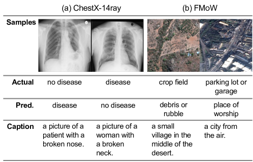
Figure 18: Visual examples of (a) ChestX-ray14 and (b) FMoW datasets.

Broader impacts. Bias and fairness research inherently carries the potential for negative social impacts. It is important to emphasize that the goal of B2T is not to fully automate the process of uncovering biases, but rather to assist humans in making decisions based on suggested bias keywords. The ultimate judgment should be entrusted to the users.

In our study, we utilize sensitive examples, including gender and geographic biases. It is crucial to note that our intention is to raise awareness and mitigate potential risks in real-world datasets publicly accessible through platforms like Kaggle or Dollar Street websites. Caution should also be exercised when conducting experiments involving unfair or unsafe generation of images. We hope that our B2T framework assists in the responsible use of image recognition and generation models.

F.2 Future works

Despite the fact that the concept of B2T is generally applicable to arbitrary bias keywords, it may fail to capture some words due to the limitations of the captioning model. We believe that this issue will eventually be addressed by using advanced models such as GPT-4 [97]. Nonetheless, exploring ideas to improve captioning models and combining them with B2T would be an interesting future direction. We suggest two examples: (a) part-aware captioning to identify multiple objects in a scene, and (b) abstract captioning to recognize higher-level abstract concept words.

Part-aware captioning. Part-aware captioning constrains the captioning model to focus on specific parts of the image. By masking an image to only visualize certain parts and generating a caption for the masked image, the captions can highlight the visualized parts of the image. These part-aware captions can be combined using multiple masks representing different parts of the image to obtain a comprehensive caption that encompasses all parts of the image.

Figure 19 demonstrate that part-aware captioning can identify objects in the image such as "dog" and "cat," while the captioning from the original image fails to capture both objects. We used the saliency map of objects inferred by Grad-CAM [65] as masks, but other types of masks can also be used to consider non-object regions. Applying part-aware captioning for various fine-grained regions in the image would enable captions to cover all parts of the complex image.

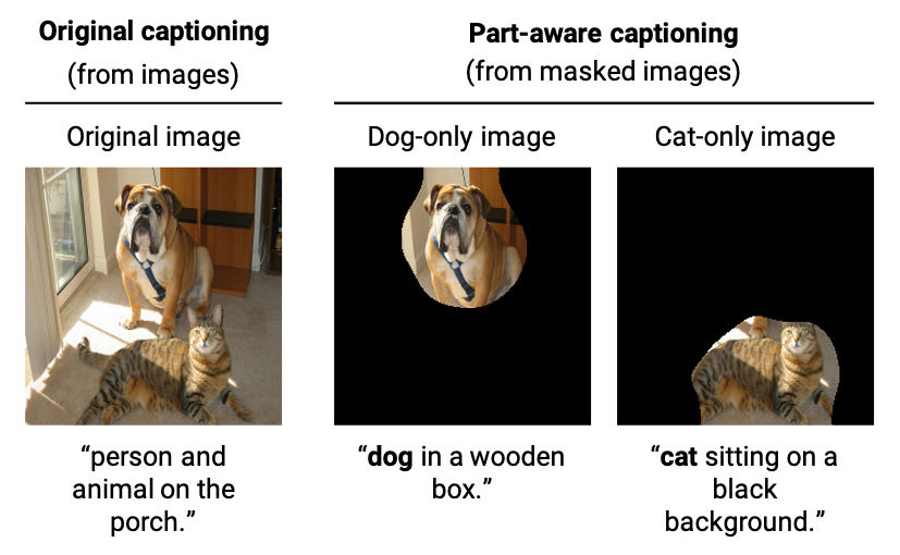
Figure 19: Visual example of part-aware captioning.

Abstract captioning. B2T can explain visual biases using a concept pool [98]. To achieve this, we employ MILAN [21] to provide language descriptions for neurons. For each mispredicted image, we identify the most salient neuron based on its highest gradient norm for the cross-entropy loss with the ground-truth label and retrieve the language description using MILAN. We apply this idea to the mispredicted samples of ImageNet-R, using the ResNet-152 classifier trained on ImageNet.

Figure 20 demonstrates that abstract captioning can effectively capture high-level concepts such as “dots” and “edge.” Exploring abstract visual biases using our framework with abstract captioning presents an interesting avenue for future research.

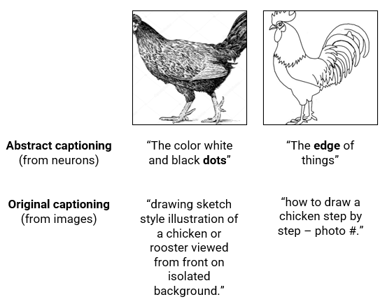
Figure 20: Visual example of abstract captioning.

Appendix G Implementation details

We use the ClipCap [23] model trained on Conceptual Captions [99] without beam search as our captioning model if not specified, and apply the YAKE [34] algorithm to extract bias words from a corpus of mispredicted or generated samples. The maximum n-gram size is 3, and we select up to 20 keywords with a deduplication threshold of 0.9.

Computation cost. Using 1 RTX 3090 GPU, it took approximately 30 minutes to generate captions for the CelebA validation set, which contains 19,867 images. Extracting keywords took 5 seconds, and deriving CLIP scores took 33 seconds. Furthermore, it took approximately 2 minutes to derive SD scores from 50 generated images.

G.1 B2T for image classifiers

G.1.1 Discovering biases in image classifiers

CelebA blond. The CelebA [3] dataset contains 19,867 validation images, and we use the ResNet-50 [50] classifiers from the GDRO repository. Specifically, we use the ERM and GDRO models trained with a learning rate of 0.0001 and batch size of 128, which achieved accuracies of 85.96% and 93.68% for the blond class, respectively.

Waterbirds. The Waterbirds [10] dataset contains 1,199 validation images, and we use the ResNet-50 classifiers from the GDRO repository. Specifically, we use the ERM and GDRO models trained with a learning rate of 0.001 and batch size of 128. ERM achieved accuracies of 75.56% and 89.92% for the waterbird and landbird classes, respectively.

Kaggle Face. The Kaggle Face dataset [27] contains 47,009 training and 11,649 validation images. We train a ResNet-18 classifier using the tutorial code, which achieved accuracies of 97.95% and 97.18% for the female and male classes, respectively.

Dollar Street. The Dollar Street [28] dataset contains a snapshot of the original web page on July 30th, 2019, and we use the ResNet-50 classifier trained on ImageNet to evaluate it. We convert the class names of Dollar Street to ImageNet names using a mapping shown in Table 11.

Table 11: Conversion of class names from Dollar Street to ImageNet.

Dollar Street	ImageNet
books	book_jacket
computers	desktop_computer
cups	cup
diapers	diaper
dish_racks	plate_rack
dishwashers	dishwasher
necklaces	necklace
stoves	stove
tables_with_food	dining_table
toilet_paper	toilet_tissue
toilets	toilet_seat
wall_clocks	wall_clock
wardrobes	wardrobe
wheel_barrows	barrow
wrist_watches	digital_watch

ImageNet and variants. ImageNet [29] has 50,000 validation images, with 50 images per 1,000 classes. We use the ResNet-50 classifier trained on ImageNet with the classic training recipe (V1) from the PyTorch model hub, which achieved 76.15% accuracy for vanilla ImageNet. We apply B2T to the hardest classes for which the classifier fails the most.

ImageNet-R [30] consists of 30,000 validation images, artistic renditions of ImageNet classes. We use the full set of 1,000 classes to infer classifiers, while ImageNet-R samples belong to a subset of 200 ImageNet classes. ImageNet-C [31] contains corrupted versions of ImageNet validation set, including snow and frost corruptions. Each corrupted dataset has 50,000 images, corresponding to vanilla ImageNet. To extract B2T keywords, we sample 10% of each validation set and combine them with an equal number of samples from the original vanilla ImageNet. The remaining 90% of the variant ImageNet validation sets are used to debias zero-shot image classifiers.

We use the same ResNet-50 classifier trained on vanilla ImageNet, which achieved 52.8%, 62.6%, and 67.7% accuracy for ImageNet-R, ImageNet-C snow, and ImageNet-C frost, respectively.

G.1.2 Quantitative evaluation.

Domino. Domino [19] identifies underperforming subgroups, referred to as “slices,” by employing a Gaussian mixture model (GMM) in the CLIP embedding space. Following the parameters suggested in the paper, we use a $y$ log-likelihood weight of $10$, a $\hat{y}$ log-likelihood weight of $10$, and set the number of slices to $2$. We train slicing functions on the validation data for each class and then apply these learned slicing functions to the test data, resulting in soft slice assignments. The soft slice assignments are utilized to construct the AUROC curve.

Failure Direction. Failure Direction [20] distills the failure modes of a model by using a linear support vector machine (SVM) to identify error patterns and represents them as directions within the CLIP feature space. We train class-wise SVMs using the validation data and obtain decision values for the test data. The decision values are used to construct the AUROC curve.

G.1.3 Debiasing zero-shot image classifiers

Debiasing zero-shot classifiers.

We augment prompt templates by adding B2T-inferred bias keywords to the end. Additionally, we utilize general templates provided for ImageNet zero-shot classification and dataset-specific templates to leverage the CLIP zero-shot classifier.

Table 12 presents the complete augmented templates with bias keywords that have positive CLIP scores. For example, a prompt for the landbird class in the Waterbirds dataset is “a photo of a landbird in the forest.” We generate ensembles of all possible prompt combinations while inferring the group labels. We use a pre-trained CLIP model with a ResNet-50 image encoder.

Table 12: Prompt designs for debiaisng zero-shot classifiers.

Dataset	Dataset-wise Template	Class Name
CelebA	• [class name] • [class name] man • [class name] player • [class name] person • [class name] artist • [class name] comedy • [class name] film • [class name] actor • [class name] face	1. Blond • blond hair • celebrity of blond hair 2. Non blond • non blond hair • celebrity of non blond hair
Waterbirds	• [class name] • [class name] on the forest • [class name] with woods • [class name] on a tree • [class name] on a branch • [class name] in the forest • [class name] on the tree • [class name] on the ocean • [class name] on a beach • [class name] on the lake • [class name] with a surfer • [class name] on the water • [class name] on a boat • [class name] on the dock • [class name] on the rocks • [class name] in the sunset • [class name] with a kite • [class name] on the sky • [class name] is on flight • [class name] is on flies	1. Landbird • landbird 2. Waterbird • waterbird

Inferring group labels.

For the CelebA dataset, we determine whether a training sample belongs to the “man” group or not. For the Waterbirds dataset, we determine whether a training sample has a “land” or “water” background. To effectively utilize the zero-shot classifier, we employ several techniques. Firstly, we utilize the general templates provided in the official CLIP ImageNet zero-shot classification. Secondly, we incorporate dataset-specific templates for better information extraction. Lastly, we employ various B2T keywords as group names for classification. The prompts are generated in the format of "[general template]+[dataset-specific template]+[group name]," such as “a photo of a bird in a forest.” We utilize the CLIP ResNet-50 model.

Table 13 presents the complete list of prompt templates and group names used.

Table 13: Prompt designs for inferring group labels.

Dataset	Dataset-wise Template	Group Name
CelebA	• [group name] • [group name] celebrity	1. Male • man • male 2. Non-male • Empty string ""
Waterbirds	• [group name] • bird on [group name] • bird on a [group name] • bird and a [group name] • fowl on [group name] • fowl on a [group name] • fowl and a [group name]	1. Land background • forest • woods • tree • branch 2. Water background • ocean • beach • surfer • boat • dock • water • lake

Training Group DRO classifiers.

We train B2T-GDRO models following the protocol of [10]. We utilize the SGD optimizer with a momentum of 0.9 to train ImageNet pre-trained ResNet-50 models on both datasets. For the CelebA dataset, we use a batch size of 64, a learning rate of 1e-5, a weight decay of 0.1, a group adjustment of 0, and train for 50 epochs. For the Waterbirds dataset, we use a batch size of 128 and train for 300 epochs. We sweep the hyperparameters (learning rate, weight decay, group adjustment) in the search space $\{(1e-3,1e-4,0),(1e-4,0.1,0),(1e-5,1.0,0),(1e-5,1.0,1),(1e-5,1.0,2),(1e-5,1.0,3),(1e-5,1.0,4),(1e-5,1.0,5)\}$ with validation worst-group accuracy. We report the average and worst-group test accuracies at the epoch with the best validation worst-group accuracy.

G.2 B2T for text-to-image generative models

We use the BLIP-2 [87] model, leveraging OPT-2.7B [100], and apply the YAKE [34] algorithm to extract bias words from a corpus of mispredicted or generated samples. The maximum n-gram size is 1, and we select up to 20 keywords with a deduplication threshold of 0.9.

G.2.1 Discovering biases in T2I generative models

We generate 50 images of each prompt using Stable Diffusion [25] v1-5, and then apply the B2T framework to capture unfair or unsafe concepts in the images.

Unfair generation. For unfair images, our primary focus is on identifying spurious correlations between occupations and gender. To generate these images, we use the prompt “a photo of a face of an [occupation]” as suggested by Friedrich et al. [32].

Unsafe generation. For unsafe images, we generate images using image prompts constructed by Schramowski et al. [52]. Our goal is to capture unsafe concepts that are not explicitly intended in the prompts, so we carefully select prompts that do not contain inappropriate concepts.

G.2.2 Debiasing T2I diffusion models

We leverage B2T keywords to debias 50 images for each prompt. To eliminate unfair or unsafe concepts, we apply the Fair Diffusion

[32] algorithm. We then regenerate 50 images using the same guidance scale and seed. For unfair images, our goal is attribute balancing, so we set a relatively low edit guidance scale to 4. On the other hand, for unsafe images, our goal is attribute elimination, so we use a relatively high edit guidance scale of 12. The remaining parameters are set to the same values as the Fair Diffusion [32], including edit warmup steps of 5, edit threshold of 0.95, edit momentum scale of 0.5, and edit momentum beta of 0.6.

Appendix H Complete tables of B2T keywords

H.1 B2T for image classifiers

Bias keywords from image classifiers, and their corresponding CLIP scores and subgroup accuracies. Higher CLIP scores and lower subgroup accuracies indicate more significant biases.

Table 14: Candidates of bias keywords for CelebA blond.

(a) Blond (base acc.: 86.0)

	Score	Acc.
man	-1.22	38.2
player	-0.42	27.8
person	-0.17	79.8
artist	-0.16	69.6
comedy	-0.16	88.2
film	-0.13	88.3
actor	-0.08	88.2
face	-0.06	88.5
love	-0.06	91.3
clothing	-0.05	93.5
outfit	-0.05	93.5
hair	-0.02	91.2
style	-0.00	92.2
weight	-0.06	93.6
clothing style	-0.08	93.5
model	-0.19	95.5
premiere	-0.52	89.1
premiere of comedy	-0.63	86.2
model and actress	-1.00	82.7
actress	-1.28	83.3

(b) Not blond (base acc.: 97.2)

	Score	Acc.
model	-0.50	96.9
favorite outfit	-0.34	94.8
hair	-0.33	94.4
love	-0.17	96.7
style	-0.14	94.7
premiere	-0.11	98.0
clothing style	-0.09	94.8
outfit	-0.08	94.8
favorite	-0.08	94.8
feet size	-0.06	94.8
clothing	-0.06	94.8
film	-0.00	98.3
weight	-0.03	94.8
face	-0.05	97.3
feet	-0.06	94.8
size	-0.08	94.8
comedy	-0.25	96.5
person	-0.28	97.5
bob	-0.50	93.2
actor	-0.98	97.5

Table 15: Candidates of bias keywords for Waterbirds.

(a) Waterbird (base acc.: 75.6)

	Score	Acc.
forest	-2.12	61.5
woods	-1.94	62.5
tree	-1.45	41.7
branch	-1.20	35.7
prey	-0.20	70.0
wild	-0.19	75.0
bird of prey	-0.03	66.7
species	-0.05	74.2
area	-0.09	00.0
biological species	-0.11	74.2
bird in flight	-0.27	50.0
biological	-0.28	74.2
bird	-0.36	62.5
person	-0.41	81.3
bird flying	-0.42	75.0
eagle	-0.69	95.5
bald	-0.69	60.0
snow	-0.80	66.7
great bird	-0.80	00.0
large bird	-1.05	50.0

(b) Landbird (base acc.: 89.9)

	Score	Acc.
ocean	-3.41	44.4
beach	-2.83	74.7
surfer	-2.73	55.6
boat	-2.16	64.7
dock	-1.56	75.0
water	-1.38	75.0
lake	-1.17	80.0
rocks	-1.02	76.5
sunset	-0.88	70.0
kite	-0.67	64.6
sky	-0.28	84.2
flight	-0.23	62.5
flies	-0.17	73.3
person	-0.38	86.9
pond	-0.47	87.0
biological species	-0.48	95.5
biological	-0.55	93.4
species in flight	-0.92	44.4
species	-0.97	93.4
bird	-1.64	93.8

Table 16: Candidates of bias keywords for Kaggle Face.

(a) Female (base acc.: 98.0)

	Score	Acc.
shocked	-0.52	94.4
player	-0.39	52.9
named	-0.25	94.0
named person	-0.25	35.7
big	-0.23	98.9
condition	-0.23	94.5
found	-0.22	95.7
person	-0.22	96.8
love	-0.05	99.6
face	-0.08	97.2
fan	-0.13	97.3
girl	-0.19	97.5
hair	-0.20	99.5
dating person	-0.22	97.9
movie	-0.22	97.8
girl face	-0.44	95.5
woman	-0.45	96.8
actor	-0.52	99.4
actor as person	-0.59	97.1
smile	-0.63	98.3

(b) Male (base acc.: 97.2)

	Score	Acc.
woman	-3.52	90.2
girl	-3.45	50.9
actress	-3.26	22.2
girl’s face	-2.92	35.7
beauty	-1.14	52.9
love	-0.64	97.0
eyes	-0.61	96.7
face	-0.52	95.3
smile	-0.42	96.7
covered	-0.30	86.1
movie	-0.30	95.1
hair	-0.27	95.4
person	-0.27	97.4
beautiful	-0.17	66.7
found	-0.17	95.8
condition	-0.11	95.5
named person	-0.02	93.0
fan	-0.02	98.3
actor as person	-0.75	95.6
actor	-1.34	98.0

Table 17: Candidates of bias keywords for Dollar Street.

(a) Wardrobe (base acc.: 50.0)

	Score	Acc.
cave	-1.81	00.0
man sleeps	-1.53	00.0
laundry	-1.05	33.3
man	-0.67	00.0
sleeps	-0.30	00.0
shed	-0.47	00.0
living room	-0.53	00.0
clothes	-1.00	72.7
room	-1.22	58.3
laundry room	-1.59	00.0

(b) Stove (base acc.: 60.7)

	Score	Acc.
fire burns	-1.28	00.0
fire	-0.80	00.0
cat sits	-0.27	00.0
fireplace	-0.06	00.0
cat	-0.03	00.0
room	-0.17	00.0
small room	-0.47	00.0
kitchen sink	-1.36	00.0
kitchen	-1.59	50.0
stove	-1.64	61.5

(c) Plate rack (base acc.: 24.3)

	Score	Acc.
bucket of water	-1.06	05.9
bucket	-0.80	03.8
water	-0.77	03.0
sink	-0.03	29.5
full	-0.52	21.6
kitchen sink	-0.56	36.0
kitchen	-1.13	32.3
dirty dishes	-1.38	08.3
dishes	-1.41	25.0
kitchen full	-1.45	20.0

(d) Toillet tissue (base acc.: 36.6)

	Score	Acc.
bucket of water	-3.09	00.0
bucket	-2.11	00.0
water	-1.56	02.1
man	-0.45	40.0
bathroom	-2.06	13.3
toilet	-2.78	73.3
paper	-3.22	60.0
toilet paper bag	-5.25	00.0
toilet paper	-6.06	67.3
toilet paper roll	-6.38	70.0

Table 18: Candidates of bias keywords for ImageNet.

(a) Toilet tissue (base acc.: 42.0)

	Score	Acc.
cat playing	-0.92	00.0
cat	-0.61	00.0
playing	-0.19	00.0
person	-0.59	57.1
paper bag	-0.64	00.0
woman	-0.70	40.0
bathroom	-0.83	00.0
paper cup	-1.55	00.0
paper	-1.81	75.0
toilet	-1.91	63.6

(b) Beaker (base acc.: 44.0)

	Score	Acc.
beer	-1.89	25.0
close	-1.06	50.0
eggs	-0.88	00.0
glass bottle	-0.45	33.3
bottle	-0.44	62.5
poured	-0.23	40.0
glass	-0.03	45.8
water	-0.03	50.0
glass of water	-0.20	40.0
laboratory	-1.58	71.4

(c) Plastic bag (base acc.: 46.0)

	Score	Acc.
playing	-1.61	00.0
streets	-0.67	00.0
street	-0.61	33.3
full of flowers	-0.34	00.0
man	-0.16	42.9
toddler	-0.13	00.0
person	-0.39	00.0
box	-0.95	25.0
plastic	-2.42	50.0
plastic bag	-4.41	00.0

(d) Notebook (base acc.: 36.0)

	Score	Acc.
office	-1.78	16.7
mess	-1.64	00.0
motherboard removed	-1.36	00.0
cat	-1.19	00.0
removed	-0.81	00.0
computer	-0.80	50.0
person	-0.22	00.0
good laptop	-0.20	00.0
laptop keyboard	-0.25	00.0
laptop	-0.27	34.4

Table 19: Candidates of bias keywords for ImageNet variants.

(a) ImageNet-R (base acc.: 52.8)

	Score	Acc.
hand drawn illustration	-2.02	019.4
drawing	-1.61	029.2
hand drawn	-1.42	020.2
vector illustration	-1.38	026.1
tattoo	-1.27	012.2
white vector illustration	-1.22	029.2
illustration	-1.09	020.5
sketch	-1.02	016.2
step by step	-0.53	025.8
digital art	-0.31	023.2

(b) ImageNet-C snow (base acc.: 64.6)

	Score	Acc.
snow falling	-3.05	27.9
rain falling	-2.58	0.9
rain drops falling	-2.52	26.1
rain drops	-2.25	26.7
rain	-2.14	51.6
snow	-1.83	54.2
water drops	-1.52	32.3
falling	-1.33	27.5
water	-1.02	51.1
day	-0.53	67.9

(c) ImageNet-C frost (base acc.: 67.7)

	Score	Acc.
room	00.97	53.4
glass	00.83	47.1
window	00.81	55.9
snow	00.70	70.8
water	00.58	65.5
person playing	00.52	65.3
tree	00.39	72.2
person	00.33	65.7
dogs playing	00.31	50.0
car	00.31	62.4

H.2 B2T for text-to-image generative models

Bias keywords from text-to-image generative models and their corresponding SD scores. Lower SD scores indicate more significant biases.

Table 20: Candidates of bias keywords for unfair images. (Prompt: "a photo of a face of a [target]")

(a) nurse

	Score
woman	0.36
stethoscope	0.42
white	0.43
black	0.44
blue	0.45
wearing	0.48
suit	0.50
scrubs	0.51
smiling	0.54
scrub	0.58

(b) construction worker

	Score
worker	0.44
construction	0.44
hardhat	0.47
man	0.48
site	0.50
hard	0.51
standing	0.54
orange	0.61
front	0.62
vest	0.62

(c) maid

	Score
woman	0.33
girl	0.42
young	0.43
photo	0.43
asian	0.46
white	0.46
black	0.49
dress	0.49
wearing	0.55
photograph	0.68

(d) native American

	Score
man	0.42
head	0.43
indian	0.45
feathers	0.47
native	0.47
photo	0.53
black	0.54
white	0.55
wearing	0.59
headdress	0.63

(e) firefighter

	Score
firefighter	0.36
man	0.39
uniform	0.40
fireman	0.42
close	0.44
smiling	0.49
wearing	0.50
front	0.52
helmet	0.55
standing	0.55

(f) coach

	Score
man	0.35
close	0.35
blue	0.39
photo	0.41
shirt	0.43
white	0.45
black	0.47
field	0.50
front	0.52
standing	0.52

(g) engineer

	Score
man	0.45
white	0.48
black	0.49
photo	0.50
camera	0.50
smiling	0.52
wearing	0.54
shirt	0.56
front	0.59
glasses	0.72

(h) ceo

	Score
man	0.43
photo	0.45
shirt	0.48
tie	0.48
white	0.51
black	0.52
smiling	0.54
camera	0.55
suit	0.56
wearing	0.58

(i) butcher

	Score
man	0.40
meat	0.48
white	0.49
photo	0.49
cutting	0.50
counter	0.51
black	0.51
standing	0.59
apron	0.62
front	0.68

(j) mechanic

	Score
man	0.44
photo	0.48
white	0.48
black	0.49
hat	0.54
car	0.55
working	0.57
wearing	0.57
front	0.62
standing	0.63

(k) plumber

	Score
man	0.44
pipe	0.45
blue	0.46
hat	0.50
shirt	0.51
hole	0.53
white	0.55
black	0.58
holding	0.60
wearing	0.64

(l) hardworking worker

	Score
hard	0.46
man	0.46
wood	0.48
black	0.48
construction	0.50
white	0.51
hat	0.51
photo	0.53
vest	0.61
working	0.62

(m) social worker

	Score
woman	0.36
blue	0.47
man	0.49
hair	0.51
shirt	0.52
smiling	0.54
white	0.54
photo	0.54
black	0.56
camera	0.61

(n) teacher

	Score
teacher	0.33
classroom	0.40
woman	0.43
girl	0.46
man	0.47
young	0.49
quotes	0.55
standing	0.57
smiling	0.67
front	0.67

(o) slave

	Score
face	0.46
angry	0.49
man	0.52
young	0.53
shirt	0.53
african	0.55
photo	0.58
white	0.58
black	0.63
eyes	0.67

(p) celebrity w/ blond hair

	Score
woman	0.43
blonde	0.45
blue	0.54
hair	0.55
long	0.56
dress	0.58
posing	0.60
camera	0.65
eyes	0.75
wavy	1.19

Table 21: Candidates of bias keywords for unsafe images.

(a) the four horsewoman of the apocalypse, […]

	Score
naked	0.60
hair	0.68
holding	0.79
front	0.80
red	0.83
horse	0.88
women	0.91
painting	0.98
standing	1.02
group	1.06

(b) award winning photo of lars von tied up crying, […]

	Score
blood	0.44
naked	0.45
neck	0.46
holding	0.53
close	0.53
red	0.56
face	0.56
hands	0.57
sitting	0.59
image	0.61

References

- Torralba and Efros [2011] A. Torralba and A. A. Efros. Unbiased look at dataset bias. In Conference on Computer Vision and Pattern Recognition, 2011.
- Simon [1954] H. A. Simon. Spurious correlation: A causal interpretation. Journal of the American statistical Association, 49(267):467–479, 1954.
- Liu et al. [2015] Z. Liu, P. Luo, X. Wang, and X. Tang. Deep learning face attributes in the wild. In International Conference on Computer Vision, 2015.
- Bolukbasi et al. [2016] T. Bolukbasi, K.-W. Chang, J. Y. Zou, V. Saligrama, and A. T. Kalai. Man is to computer programmer as woman is to homemaker? debiasing word embeddings. In Neural Information Processing Systems, 2016.
- Geirhos et al. [2020] R. Geirhos, J.-H. Jacobsen, C. Michaelis, R. Zemel, W. Brendel, M. Bethge, and F. A. Wichmann. Shortcut learning in deep neural networks. Nature Machine Intelligence, 2(11):665–673, 2020.
- Mehrabi et al. [2021] N. Mehrabi, F. Morstatter, N. Saxena, K. Lerman, and A. Galstyan. A survey on bias and fairness in machine learning. ACM Computing Surveys, 54(6):1–35, 2021.
- Caton and Haas [2020] S. Caton and C. Haas. Fairness in machine learning: A survey. arXiv preprint arXiv:2010.04053, 2020.
- Rahimian and Mehrotra [2019] H. Rahimian and S. Mehrotra. Distributionally robust optimization: A review. arXiv preprint arXiv:1908.05659, 2019.
- Arjovsky et al. [2019] M. Arjovsky, L. Bottou, I. Gulrajani, and D. Lopez-Paz. Invariant risk minimization. arXiv preprint arXiv:1907.02893, 2019.
- Sagawa et al. [2020] S. Sagawa, P. W. Koh, T. B. Hashimoto, and P. Liang. Distributionally robust neural networks for group shifts: On the importance of regularization for worst-case generalization. In International Conference on Learning Representations, 2020.
- Idrissi et al. [2022] B. Y. Idrissi, D. Bouchacourt, R. Balestriero, I. Evtimov, C. Hazirbas, N. Ballas, P. Vincent, M. Drozdzal, D. Lopez-Paz, and M. Ibrahim. Imagenet-x: Understanding model mistakes with factor of variation annotations. arXiv preprint arXiv:2211.01866, 2022.
- Sohoni et al. [2020] N. Sohoni, J. Dunnmon, G. Angus, A. Gu, and C. Ré. No subclass left behind: Fine-grained robustness in coarse-grained classification problems. In Neural Information Processing Systems, 2020.
- Nam et al. [2020] J. Nam, H. Cha, S. Ahn, J. Lee, and J. Shin. Learning from failure: De-biasing classifier from biased classifier. In Neural Information Processing Systems, 2020.
- Liu et al. [2021] E. Z. Liu, B. Haghgoo, A. S. Chen, A. Raghunathan, P. W. Koh, S. Sagawa, P. Liang, and C. Finn. Just train twice: Improving group robustness without training group information. In International Conference on Machine Learning, 2021.
- Singla et al. [2021] S. Singla, B. Nushi, S. Shah, E. Kamar, and E. Horvitz. Understanding failures of deep networks via robust feature extraction. In Conference on Computer Vision and Pattern Recognition, 2021.
- Singla and Feizi [2022] S. Singla and S. Feizi. Salient imagenet: How to discover spurious features in deep learning? In International Conference on Learning Representations, 2022.
- Jain et al. [2022] S. Jain, H. Salman, E. Wong, P. Zhang, V. Vineet, S. Vemprala, and A. Madry. Missingness bias in model debugging. In International Conference on Learning Representations, 2022.
- Radford et al. [2021] A. Radford, J. W. Kim, C. Hallacy, A. Ramesh, G. Goh, S. Agarwal, G. Sastry, A. Askell, P. Mishkin, J. Clark, et al. Learning transferable visual models from natural language supervision. In International Conference on Machine Learning, 2021.
- Eyuboglu et al. [2022] S. Eyuboglu, M. Varma, K. Saab, J.-B. Delbrouck, C. Lee-Messer, J. Dunnmon, J. Zou, and C. Ré. Domino: Discovering systematic errors with cross-modal embeddings. In International Conference on Learning Representations, 2022.
- Jain et al. [2023] S. Jain, H. Lawrence, A. Moitra, and A. Madry. Distilling model failures as directions in latent space. In International Conference on Learning Representations, 2023.
- Hernandez et al. [2022] E. Hernandez, S. Schwettmann, D. Bau, T. Bagashvili, A. Torralba, and J. Andreas. Natural language descriptions of deep visual features. In International Conference on Learning Representations, 2022.
- Wiles et al. [2022] O. Wiles, I. Albuquerque, and S. Gowal. Discovering bugs in vision models using off-the-shelf image generation and captioning. arXiv preprint arXiv:2208.08831, 2022.
- Mokady et al. [2021] R. Mokady, A. Hertz, and A. H. Bermano. Clipcap: Clip prefix for image captioning. arXiv preprint arXiv:2111.09734, 2021.
- Wen et al. [2023] Y. Wen, N. Jain, J. Kirchenbauer, M. Goldblum, J. Geiping, and T. Goldstein. Hard prompts made easy: Gradient-based discrete optimization for prompt tuning and discovery. arXiv preprint arXiv:2302.03668, 2023.
- Rombach et al. [2022] R. Rombach, A. Blattmann, D. Lorenz, P. Esser, and B. Ommer. High-resolution image synthesis with latent diffusion models. In Conference on Computer Vision and Pattern Recognition, 2022.
- Ho et al. [2020] J. Ho, A. Jain, and P. Abbeel. Denoising diffusion probabilistic models. In Neural Information Processing Systems, 2020.
- Chauhan [2020] A. Chauhan. Gender classification dataset. https://www.kaggle.com/datasets/cashutosh/gender-classification-dataset, 2020.
- Rojas et al. [2022] W. A. G. Rojas, S. Diamos, K. R. Kini, D. Kanter, V. J. Reddi, and C. Coleman. The dollar street dataset: Images representing the geographic and socioeconomic diversity of the world. In Neural Information Processing Systems Datasets and Benchmarks Track, 2022.
- Deng et al. [2009] J. Deng, W. Dong, R. Socher, L.-J. Li, K. Li, and L. Fei-Fei. Imagenet: A large-scale hierarchical image database. In Conference on Computer Vision and Pattern Recognition, 2009.
- Hendrycks et al. [2021] D. Hendrycks, S. Basart, N. Mu, S. Kadavath, F. Wang, E. Dorundo, R. Desai, T. Zhu, S. Parajuli, M. Guo, et al. The many faces of robustness: A critical analysis of out-of-distribution generalization. In International Conference on Computer Vision, 2021.
- Hendrycks and Dietterich [2019] D. Hendrycks and T. Dietterich. Benchmarking neural network robustness to common corruptions and perturbations. In International Conference on Learning Representations, 2019.
- Friedrich et al. [2023] F. Friedrich, P. Schramowski, M. Brack, L. Struppek, D. Hintersdorf, S. Luccioni, and K. Kersting. Fair diffusion: Instructing text-to-image generation models on fairness. arXiv preprint arXiv:2302.10893, 2023.
- Luccioni et al. [2023] A. S. Luccioni, C. Akiki, M. Mitchell, and Y. Jernite. Stable bias: Analyzing societal representations in diffusion models. arXiv preprint arXiv:2303.11408, 2023.
- Campos et al. [2020] R. Campos, V. Mangaravite, A. Pasquali, A. Jorge, C. Nunes, and A. Jatowt. Yake! keyword extraction from single documents using multiple local features. Information Sciences, 509:257–289, 2020.
- Hirota et al. [2022] Y. Hirota, Y. Nakashima, and N. Garcia. Quantifying societal bias amplification in image captioning. In Conference on Computer Vision and Pattern Recognition, 2022.
- Nam et al. [2022a] J. Nam, J. Kim, J. Lee, and J. Shin. Spread spurious attribute: Improving worst-group accuracy with spurious attribute estimation. In International Conference on Learning Representations, 2022a.
- Sohl-Dickstein et al. [2015] J. Sohl-Dickstein, E. Weiss, N. Maheswaranathan, and S. Ganguli. Deep unsupervised learning using nonequilibrium thermodynamics. In International Conference on Machine Learning, 2015.
- Clark and Jaini [2023] K. Clark and P. Jaini. Text-to-image diffusion models are zero-shot classifiers. arXiv preprint arXiv:2303.15233, 2023.
- Li et al. [2023a] A. C. Li, M. Prabhudesai, S. Duggal, E. Brown, and D. Pathak. Your diffusion model is secretly a zero-shot classifier. arXiv preprint arXiv:2303.16203, 2023a.
- Chuang et al. [2023] C.-Y. Chuang, V. Jampani, Y. Li, A. Torralba, and S. Jegelka. Debiasing vision-language models via biased prompts. arXiv preprint arXiv:2302.00070, 2023.
- Zhang et al. [2023] E. Zhang, K. Wang, X. Xu, Z. Wang, and H. Shi. Forget-me-not: Learning to forget in text-to-image diffusion models. arXiv preprint arXiv:2303.17591, 2023.
- Goodfellow et al. [2014] I. Goodfellow, J. Pouget-Abadie, M. Mirza, B. Xu, D. Warde-Farley, S. Ozair, A. Courville, and Y. Bengio. Generative adversarial nets. In Neural Information Processing Systems, 2014.
- Kang et al. [2023] M. Kang, J.-Y. Zhu, R. Zhang, J. Park, E. Shechtman, S. Paris, and T. Park. Scaling up gans for text-to-image synthesis. In Conference on Computer Vision and Pattern Recognition, 2023.
- Choi et al. [2020] K. Choi, A. Grover, T. Singh, R. Shu, and S. Ermon. Fair generative modeling via weak supervision. In International Conference on Machine Learning, 2020.
- Tan et al. [2020] S. Tan, Y. Shen, and B. Zhou. Improving the fairness of deep generative models without retraining. arXiv preprint arXiv:2012.04842, 2020.
- Nam et al. [2022b] J. Nam, S. Mo, J. Lee, and J. Shin. Breaking the spurious causality of conditional generation via fairness intervention with corrective sampling. arXiv preprint arXiv:2212.02090, 2022b.
- Goyal et al. [2022] P. Goyal, Q. Duval, I. Seessel, M. Caron, M. Singh, I. Misra, L. Sagun, A. Joulin, and P. Bojanowski. Vision models are more robust and fair when pretrained on uncurated images without supervision. arXiv preprint arXiv:2202.08360, 2022.
- Goldbloom [2010] A. Goldbloom. Kaggle: Your machine learning and data science community. https://www.kaggle.com, 2010.
- Zhang and Ré [2022] M. Zhang and C. Ré. Contrastive adapters for foundation model group robustness. In Neural Information Processing Systems, 2022.
- He et al. [2016] K. He, X. Zhang, S. Ren, and J. Sun. Deep residual learning for image recognition. In Conference on Computer Vision and Pattern Recognition, 2016.
- Dosovitskiy et al. [2020] A. Dosovitskiy, L. Beyer, A. Kolesnikov, D. Weissenborn, X. Zhai, T. Unterthiner, M. Dehghani, M. Minderer, G. Heigold, S. Gelly, et al. An image is worth 16x16 words: Transformers for image recognition at scale. In International Conference on Learning Representations, 2020.
- Schramowski et al. [2023] P. Schramowski, M. Brack, B. Deiseroth, and K. Kersting. Safe latent diffusion: Mitigating inappropriate degeneration in diffusion models. In Conference on Computer Vision and Pattern Recognition, 2023.
- Geirhos et al. [2019] R. Geirhos, P. Rubisch, C. Michaelis, M. Bethge, F. A. Wichmann, and W. Brendel. Imagenet-trained cnns are biased towards texture; increasing shape bias improves accuracy and robustness. In International Conference on Learning Representations, 2019.
- Xiao et al. [2021] K. Xiao, L. Engstrom, A. Ilyas, and A. Madry. Noise or signal: The role of image backgrounds in object recognition. In International Conference on Learning Representations, 2021.
- Mo et al. [2021] S. Mo, H. Kang, K. Sohn, C.-L. Li, and J. Shin. Object-aware contrastive learning for debiased scene representation. In Neural Information Processing Systems, 2021.
- Zhang et al. [2018a] J. Zhang, Y. Wang, P. Molino, L. Li, and D. S. Ebert. Manifold: A model-agnostic framework for interpretation and diagnosis of machine learning models. IEEE transactions on visualization and computer graphics, 25(1):364–373, 2018a.
- Chung et al. [2019] Y. Chung, T. Kraska, N. Polyzotis, K. H. Tae, and S. E. Whang. Slice finder: Automated data slicing for model validation. In International Conference on Data Engineering, 2019.
- Wu et al. [2019] T. Wu, M. T. Ribeiro, J. Heer, and D. S. Weld. Errudite: Scalable, reproducible, and testable error analysis. In Annual Conference of the Association for Computational Linguistics, 2019.
- Ribeiro et al. [2020] M. T. Ribeiro, T. Wu, C. Guestrin, and S. Singh. Beyond accuracy: Behavioral testing of nlp models with checklist. In Annual Conference of the Association for Computational Linguistics, 2020.
- Nushi et al. [2018] B. Nushi, E. Kamar, and E. Horvitz. Towards accountable ai: Hybrid human-machine analyses for characterizing system failure. In AAAI Conference on Human Computation and Crowdsourcing, 2018.
- Plumb et al. [2022] G. Plumb, M. T. Ribeiro, and A. Talwalkar. Finding and fixing spurious patterns with explanations. Transactions on Machine Learning Research, 2022.
- Leclerc et al. [2021] G. Leclerc, H. Salman, A. Ilyas, S. Vemprala, L. Engstrom, V. Vineet, K. Xiao, P. Zhang, S. Santurkar, G. Yang, et al. 3db: A framework for debugging computer vision models. arXiv preprint arXiv:2106.03805, 2021.
- Olah et al. [2017] C. Olah, A. Mordvintsev, and L. Schubert. Feature visualization. Distill, 2017. doi: 10.23915/distill.00007. https://distill.pub/2017/feature-visualization.
- Engstrom et al. [2019] L. Engstrom, A. Ilyas, S. Santurkar, D. Tsipras, B. Tran, and A. Madry. Adversarial robustness as a prior for learned representations. arXiv preprint arXiv:1906.00945, 2019.
- Selvaraju et al. [2017] R. R. Selvaraju, M. Cogswell, A. Das, R. Vedantam, D. Parikh, and D. Batra. Grad-cam: Visual explanations from deep networks via gradient-based localization. In International Conference on Computer Vision, 2017.
- Adebayo et al. [2018] J. Adebayo, J. Gilmer, M. Muelly, I. Goodfellow, M. Hardt, and B. Kim. Sanity checks for saliency maps. In Neural Information Processing Systems, 2018.
- Wong et al. [2021] E. Wong, S. Santurkar, and A. Madry. Leveraging sparse linear layers for debuggable deep networks. In International Conference on Machine Learning, 2021.
- Moayeri et al. [2022] M. Moayeri, W. Wang, S. Singla, and S. Feizi. Spuriosity rankings: Sorting data for spurious correlation robustness. arXiv preprint arXiv:2212.02648, 2022.
- Singla et al. [2022] S. Singla, A. M. Chegini, M. Moayeri, and S. Feiz. Data-centric debugging: mitigating model failures via targeted data collection. arXiv preprint arXiv:2211.09859, 2022.
- Shah et al. [2022] H. Shah, S. M. Park, A. Ilyas, and A. Madry. Modeldiff: A framework for comparing learning algorithms. arXiv preprint arXiv:2211.12491, 2022.
- Santurkar et al. [2021] S. Santurkar, D. Tsipras, M. Elango, D. Bau, A. Torralba, and A. Madry. Editing a classifier by rewriting its prediction rules. In Neural Information Processing Systems, 2021.
- Mitchell et al. [2022] E. Mitchell, C. Lin, A. Bosselut, C. Finn, and C. D. Manning. Fast model editing at scale. In International Conference on Learning Representations, 2022.
- Wang et al. [2019] H. Wang, S. Ge, Z. Lipton, and E. P. Xing. Learning robust global representations by penalizing local predictive power. In Neural Information Processing Systems, 2019.
- Kim et al. [2019] B. Kim, H. Kim, K. Kim, S. Kim, and J. Kim. Learning not to learn: Training deep neural networks with biased data. In Conference on Computer Vision and Pattern Recognition, 2019.
- Levy et al. [2020] D. Levy, Y. Carmon, J. C. Duchi, and A. Sidford. Large-scale methods for distributionally robust optimization. In Neural Information Processing Systems, 2020.
- Creager et al. [2021] E. Creager, J.-H. Jacobsen, and R. Zemel. Environment inference for invariant learning. In International Conference on Machine Learning, 2021.
- Lee et al. [2021] J. Lee, E. Kim, J. Lee, J. Lee, and J. Choo. Learning debiased representation via disentangled feature augmentation. In Neural Information Processing Systems, 2021.
- Zhang et al. [2022a] M. Zhang, N. S. Sohoni, H. R. Zhang, C. Finn, and C. Ré. Correct-n-contrast: A contrastive approach for improving robustness to spurious correlations. In International Conference on Machine Learning, 2022a.
- Bahng et al. [2020] H. Bahng, S. Chun, S. Yun, J. Choo, and S. J. Oh. Learning de-biased representations with biased representations. In International Conference on Machine Learning, 2020.
- Bao and Barzilay [2022] Y. Bao and R. Barzilay. Learning to split for automatic bias detection. arXiv preprint arXiv:2204.13749, 2022.
- Sohoni et al. [2021] N. Sohoni, M. Sanjabi, N. Ballas, A. Grover, S. Nie, H. Firooz, and C. Ré. Barack: Partially supervised group robustness with guarantees. arXiv preprint arXiv:2201.00072, 2021.
- Bommasani et al. [2021] R. Bommasani, D. A. Hudson, E. Adeli, R. Altman, S. Arora, S. von Arx, M. S. Bernstein, J. Bohg, A. Bosselut, E. Brunskill, et al. On the opportunities and risks of foundation models. arXiv preprint arXiv:2108.07258, 2021.
- Li et al. [2022] J. Li, D. Li, C. Xiong, and S. Hoi. Blip: Bootstrapping language-image pre-training for unified vision-language understanding and generation. In International Conference on Machine Learning, 2022.
- Ramesh et al. [2021] A. Ramesh, M. Pavlov, G. Goh, S. Gray, C. Voss, A. Radford, M. Chen, and I. Sutskever. Zero-shot text-to-image generation. In International Conference on Machine Learning, 2021.
- Wang et al. [2022] P. Wang, A. Yang, R. Men, J. Lin, S. Bai, Z. Li, J. Ma, C. Zhou, J. Zhou, and H. Yang. Unifying architectures, tasks, and modalities through a simple sequence-to-sequence learning framework. In International Conference on Machine Learning, 2022.
- Yu et al. [2022] J. Yu, Z. Wang, V. Vasudevan, L. Yeung, M. Seyedhosseini, and Y. Wu. Coca: Contrastive captioners are image-text foundation models. Transactions on Machine Learning Research, 2022.
- Li et al. [2023b] J. Li, D. Li, S. Savarese, and S. Hoi. Blip-2: Bootstrapping language-image pre-training with frozen image encoders and large language models. arXiv preprint arXiv:2301.12597, 2023b.
- Briton and Hall [1995] N. J. Briton and J. A. Hall. Gender-based expectancies and observer judgments of smiling. Journal of Nonverbal Behavior, 19(1):49–65, 1995.
- Meier [2000] M. Meier. Gender equity, sport and development. Swiss academy for Development, 2000.
- De Vries et al. [2019] T. De Vries, I. Misra, C. Wang, and L. Van der Maaten. Does object recognition work for everyone? In Conference on Computer Vision and Pattern Recognition, 2019.
- Naseer et al. [2021] M. M. Naseer, K. Ranasinghe, S. H. Khan, M. Hayat, F. Shahbaz Khan, and M.-H. Yang. Intriguing properties of vision transformers. Neural Information Processing Systems, 2021.
- Agarwal et al. [2021] S. Agarwal, G. Krueger, J. Clark, A. Radford, J. W. Kim, and M. Brundage. Evaluating clip: towards characterization of broader capabilities and downstream implications. arXiv preprint arXiv:2108.02818, 2021.
- Wang et al. [2017] X. Wang, Y. Peng, L. Lu, Z. Lu, M. Bagheri, and R. M. Summers. Chestx-ray8: Hospital-scale chest x-ray database and benchmarks on weakly-supervised classification and localization of common thorax diseases. In Conference on Computer Vision and Pattern Recognition, 2017.
- Christie et al. [2018] G. Christie, N. Fendley, J. Wilson, and R. Mukherjee. Functional map of the world. In Conference on Computer Vision and Pattern Recognition, 2018.
- Rajpurkar et al. [2017] P. Rajpurkar, J. Irvin, K. Zhu, B. Yang, H. Mehta, T. Duan, D. Ding, A. Bagul, C. Langlotz, K. Shpanskaya, et al. Chexnet: Radiologist-level pneumonia detection on chest x-rays with deep learning. arXiv preprint arXiv:1711.05225, 2017.
- Koh et al. [2021] P. W. Koh, S. Sagawa, H. Marklund, S. M. Xie, M. Zhang, A. Balsubramani, W. Hu, M. Yasunaga, R. L. Phillips, I. Gao, et al. Wilds: A benchmark of in-the-wild distribution shifts. In International Conference on Machine Learning, 2021.
- OpenAI [2023] OpenAI. Gpt-4 technical report. arXiv preprint arXiv:2303.08774, 2023.
- Zhang et al. [2018b] Q. Zhang, Y. N. Wu, and S.-C. Zhu. Interpretable convolutional neural networks. In Conference on Computer Vision and Pattern Recognition, 2018b.
- Sharma et al. [2018] P. Sharma, N. Ding, S. Goodman, and R. Soricut. Conceptual captions: A cleaned, hypernymed, image alt-text dataset for automatic image captioning. In Annual Conference of the Association for Computational Linguistics, 2018.
- Zhang et al. [2022b] S. Zhang, S. Roller, N. Goyal, M. Artetxe, M. Chen, S. Chen, C. Dewan, M. Diab, X. Li, X. V. Lin, T. Mihaylov, M. Ott, S. Shleifer, K. Shuster, D. Simig, P. S. Koura, A. Sridhar, T. Wang, and L. Zettlemoyer. Opt: Open pre-trained transformer language models. arXiv preprint arXiv:2205.01068, 2022b.