Covariant light-front approach for $B_{c}$ decays into charmonium: implications on form factors and branching ratios

Abstract

In this work, we investigate the form factors of $B_{c}$ decays into $J/\Psi,\psi(2S,3S),\eta_{c},$ $\eta_{c}(2S,3S),\chi_{c0},\chi_{c1},h_{c}$ and $X(3872)$ mesons in the covariant light-front quark model (CLFQM). For the purpose of the branching ratio calculation, the form factors of $B_{c}\to D^{(*)},D^{(*)}_{s}$ transitions are also included. In order to obtain the form factors for the physical transition processes, we need to extend these form factors from the space-like region to the time-like region. The $q^{2}$-dependence for each transition form factor is also plotted. Then, using the factorization method, we calculate the branching ratios of 80 $B_{c}$ decay channels with a charmonium involved in each mode. Most of our predictions are comparable to the results given by other approaches. As to the decays with the radially excited-state S-wave charmonia involved, such as $\psi(2S,3S)$ and $\eta_{c}(2S,3S)$, two sets of parameters for their light-front wave functions, corresponding to scenario I (SI) and scenario II (SII), are adopted to calculate the branching ratios. By comparing with the future experimental data, one can discriminate which parameters are more favored.

I Introduction

During the period from the 1970s to 1980s, the light-front quark model (LFQM) was developed terent ; chung to deal with nonperturbative physical quantities such as decay constants, transition form factors, and so on. This relativistic quark model is based on a light-front formalism dirac and quantum chromodynamics (QCD) light-front quantization brodsky . The LFQM can provide a relativistic treatment of the hadron momentum and fully treatment of the quark spin by using the so-called Melosh rotation. At the same time, the light-front wave functions are independent of the hadron momentum and thus are manifestly Lorentz invariant. Equipped with these advantages, the LFQM becomes a convenient approach and has been employed to calculate decay constants and form factors jaus90 ; jaus91 ; ji92 ; cheng97 ; cheng98 . While under the LFQM, the constituent quark and antiquark in a bound state are required to be on their mass shells, which makes degrees of freedom of light-front momentum become three and the Lorentz covariance of the matrix elements to be lost. The usual practice is only taking the plus component ($\mu=+$) of the current matrix elements, which will miss the zero-mode contributions. However, lacking the zero-mode contributions sometimes affects the calculation accuracy. Unfortunately, such conventional LFQM approach with defect is powerless to calculate the zero-mode contributions. At the end of the twentieth century, Jaus put forward the covariant Light-Front quark model (CLFQM) jaus . The previous LFQM is usually called the standard Light-Front quark model (SLFQM) jaus . The CLFQM is more convincing than the SLFQM. In the CLFQM approach jaus , when evaluating the light-front matrix element from the momentum loop integral by a light-front decomposition to the internal momentum and carrying out the integration over the minus component ($p^{-}=p^{0}-p^{3}$) by means of contour methods, one will encounter additional spurious contribution proportional to the light-like vector $\omega^{\mu}=(0,2,0_{\bot})$, which violates the covariance. While this spurious contribution is just canceled by the zero-mode contribution, at the same time the covariance of the current matrix elements is restored, and all the problems can be resolved. Since the popular CLFQM was proposed, it has been widely used to study the form factors and the decay constants of the ground-state S-wave and low-lying P-wave mesons, and is further applied to phenomenological studies about $B_{c}$ decays hycheng ; wwang ; wwang1 ; wwang2 ; Ke13 . Certainly, there still exist some discussions about the self-consistency of the CLFQM, for example, the decay constant of the vector meson, which is different as a result of extracting from different polarization (longitudinal and transverse) states choi14 ; chang18 ; chang20 ; chang21 .

$B_{c}$ meson decays have received extensive attention because of its unique structure in the Standard Model. The $B_{c}$ meson is the only heavy meson composed of two heavy quarks with different flavors (b and c), which cannot annihilate into gluons (photon) via strong (electromagnetic) interaction. Decays of the $B_{c}$ meson occur only via weak interaction, which includes three types at the quark level, the $b\to c(u)$, $c\to s(d)$ transitions, and the weak annihlilations. Although the phase space of the $c$ quark decays is much smaller than that of the $b$ quark decays, the Cabibbo-Kobayashi-Maskawa (CKM) matrix elements are greatly in favor of the $c$ quark decays (i.e., $|V_{cs}|\gg|V_{cb}|,|V_{cd}|\gg|V_{ub}|$), which provide about $70\%$ of the $B_{c}$ decay width, while the $b$ quark decays and the weak annihilations only amount to about $20\%$ and $10\%$, respectively gouz . On the experimental side, since the $B_{c}$ meson was first discovered by the Collider Detector at Fermilab (CDF) collaboration via the decay of $B_{c}\to J/\Psi l\nu$ in 1.8 TeV $p\bar{p}$ collisions at the Fermilab Tevatron, many $B_{c}$ decay channels have been observed by the Large Hadron Collider beauty (LHCb) collaboration, such as $B_{c}^{+}\to J/\Psi\pi^{+}\pi^{-}\pi^{+}$ aajj1 , $B_{c}^{+}\to J/\Psi\pi^{+}$ aajj11 , $B_{c}^{+}\to J/\Psi K^{+}$ aajj2 , $B_{c}^{+}\to J/\Psi D_{s}^{(*)+}$ aajj3 , $B_{c}^{+}\to J/\Psi K^{+}K^{-}\pi^{+}$ aajj4 , and $B_{c}^{+}\to B^{0}_{s}\pi^{+}$ aajj5 . The inclusive production cross section of the $B_{c}$ meson at the LHC is estimated to be at a level of $1\mu b$ for $\sqrt{14}$ TeV. This means that around $\mathcal{O}(10^{9})$ $B_{c}$ events with a luminosity of $1fb^{-1}$ can be provided gao10 , which are sufficient for studying the $B_{c}$ meson decays. On the theoretical side, many theoretical methods have been used to study the $B_{c}$ meson decays to charmonium states, such as the perturbation QCD (PQCD) approach Zhu ; Rui:2016opu , the generalized factorization (GF) approach Hsiao:2016pml , the QCD factorization (QCDF) approach chang182 , the QCD sum rule (QCDSR) approach V , the Bethe-Salpter Equation approach chang , the relativistic quark model (RQM) Ivanov ; kang , and nonrelativistic QCD approach(NRQCD) Qiao .

The development of the theoretical and experimental aspects of the $B_{c}$ meson physics motivates us to investigate the $B_{c}$ weak decays with a charmonium involved in each mode. In Sect.2, we recapitulate the CLFQM, including the definitions of the decay constants and the relevant formulae of $B_{c}$ to charmonium or charmed meson transition form factors. In Sect.3, after determining the shape parameters $\beta^{\prime}$ using the corresponding decay constants, we provide the numerical results of $B_{c}$ transition form factors and their $q^{2}$ dependence. Then, using the transition form factors, we calculate the branching ratios of $B_{c}$ decays with a charmonium meson involved in each mode. In addition, detailed data analysis and discussion, including a comparison with the other model calculations, are carried out. The conclusions are presented in the final part.

Table 1: Feynman rules for the vertices $i\Gamma^{\prime}_{M}$ of the incoming meson-quark-antiquark, where $p^{\prime}_{1}$ and $p_{2}$ are the quark and antiquark momenta, respectively.

$M\left({}^{2S+1}L_{J}\right)$	$i\Gamma_{M}^{\prime}$
$\text{ pseudoscalar }\left({}^{1}S_{0}\right)$	$H_{P}^{\prime}\gamma_{5}$
$\text{ vector }\left({}^{3}S_{1}\right)$	$iH_{V}^{\prime}\left[\gamma_{\mu}-\frac{1}{W_{V}^{\prime}}\left(p_{1}^{\prime}-p_{2}\right)_{\mu}\right]$
$\text{ scalar }\left({}^{3}P_{0}\right)$	$-iH_{S}^{\prime}$
$\text{ axial }\left({}^{3}P_{1}\right)$	$-iH_{3_{A}}^{\prime}\left[\gamma_{\mu}+\frac{1}{W_{3_{A}}^{\prime}}\left(p_{1}^{\prime}-p_{2}\right)_{\mu}\right]\gamma_{5}$
$\text{ axial }\left({}^{1}P_{1}\right)$	$-iH_{1_{A}}^{\prime}\left[\frac{1}{W_{1_{A}}^{\prime}}\left(p_{1}^{\prime}-p_{2}\right)_{\mu}\right]\gamma_{5}$

II Formalism

II.1 Covariant light-front quark model

Under the covariant light-front quark model, the light-front coordinates of a momentum $p$ are used, $p=(p^{-},p^{+},p_{\perp})$, with $p^{\pm}=p^{0}\pm p_{z},$ and $p^{2}=p^{+}p^{-}-p^{2}_{\perp}$. The Feynman diagrams for $B_{c}$ meson decay and transition amplitudes are shown in Fig. 1. The incoming (outgoing) meson has mass $M^{\prime}(M^{\prime\prime})$ with the momentum $P^{\prime}=p_{1}^{\prime}+p_{2}(P^{\prime\prime}=p_{1}^{\prime\prime}+p_{2})$, where $p_{1}^{\prime(\prime\prime)}$ and $p_{2}$ are the momenta of the quark and antiquark inside the incoming (outgoing) meson with mass $m_{1}^{\prime(\prime\prime)}$and $m_{2}$, respectively. Here, we use the same notation as those in Refs. jaus ; hycheng and $M^{\prime}=m_{B_{c}}$ for $B_{c}$ meson decays. These momenta can be expressed in terms of the internal variables $(x_{i},p{{}^{\prime}}_{\perp})$ as

$$p_{1,2}^{\prime+}=x_{1,2}P^{\prime+},\quad p_{1,2\perp}^{\prime}=x_{1,2}P_{\perp}^{\prime}\pm p_{\perp}^{\prime}$$ (1)

with $x_{1}+x_{2}=1$. Using these internal variables, we can define some quantities for the incoming meson which will be used in the following calculations:

$$M_{0}^{\prime 2} = \left(e_{1}^{\prime}+e_{2}\right)^{2}=\frac{p_{\perp}^{\prime 2}+m_{1}^{\prime 2}}{x_{1}}+\frac{p_{\perp}^{2}+m_{2}^{2}}{x_{2}},\quad\widetilde{M}_{0}^{\prime}=\sqrt{M_{0}^{\prime 2}-\left(m_{1}^{\prime}-m_{2}\right)^{2}},$$

$$e_{i}^{(\prime)} = \sqrt{m_{i}^{(\prime)2}+p_{\perp}^{\prime 2}+p_{z}^{\prime 2}},\quad\quad p_{z}^{\prime}=\frac{x_{2}M_{0}^{\prime}}{2}-\frac{m_{2}^{2}+p_{\perp}^{\prime 2}}{2x_{2}M_{0}^{\prime}},$$ (2)

where $M^{\prime}_{0}$ is the kinetic invariant mass of the incoming meson and can be expressed as the energies of the quark and the antiquark $e^{(\prime)}_{i}$. It is similar to the case of the outgoing meson.

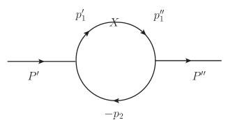
Figure 1: Feynman diagrams for $B_{c}$ decay (left) and transition (right) amplitudes, where $P^{\prime(\prime\prime)}$ is the incoming (outgoing) meson momentum, $p^{\prime(\prime\prime)}_{1}$ is the quark momentum, $p_{2}$ is the antiquark momentum and X denotes the vector or axial vector transition vertex.

To calculate the amplitudes for the transition form factors, we need the Feynman rules for the meson-quark-antiquark vertices ($i\Gamma^{\prime}_{M}(M=P,V,A,S)$), which are listed in Tab. 1. It is noted that for the outgoing meson, we should use $i(\gamma_{0}\Gamma^{\prime{\dagger}}_{M}\gamma_{0})$ for the relevant vertices. The $B_{c}\to M$ ($M$ denotes a pseudoscalar (P), a vector (V), an axial-vector (A) or a scalar (S) meson) form factors induced by vector and aixal-vector currents are defined as

$$\left\langle P\left(P^{\prime\prime}\right)\left|V_{\mu}\right|B_{c}\left(P^{\prime}\right)\right\rangle = f_{+}(q^{2})P_{\mu}+f_{-}(q^{2})q_{\mu},$$ (3)

$$\left\langle V\left(P^{\prime\prime},\varepsilon\right)\left|V_{\mu}\right|B_{c}\left(P^{\prime}\right)\right\rangle = \epsilon_{\mu\nu\alpha\beta}\varepsilon^{*\nu}P^{\alpha}q^{\beta}g(q^{2}),$$ (4)

$$\left\langle V\left(P^{\prime\prime},\varepsilon\right)\left|A_{\mu}\right|B_{c}\left(P^{\prime}\right)\right\rangle = -i\left\{\varepsilon_{\mu}^{*}f(q^{2})+\varepsilon^{*}\cdot P\left[P_{\mu}a_{+}(q^{2})+q_{\mu}a_{-}(q^{2})\right]\right\},$$ (5)

$$\left\langle\;{}^{1}A\left(P^{\prime\prime},\varepsilon\right)\left|A_{\mu}\right|B_{c}\left(P^{\prime}\right)\right\rangle =- q^{\;{}^{1}A}(q^{2})\epsilon_{\mu\nu\alpha\beta}\varepsilon^{*\nu}P^{\alpha}q^{\beta},$$ (6)

$$\left\langle\;{}^{1}A\left(P^{\prime\prime},\varepsilon\right)\left|V_{\mu}\right|B_{c}\left(P^{\prime}\right)\right\rangle = i\left\{l^{\;{}^{1}A}(q^{2})\varepsilon_{\mu}^{*}+\varepsilon^{*}\cdot P\left[P_{\mu}c^{\;{}^{1}A}_{+}(q^{2})+q_{\mu}c^{\;{}^{1}A}_{-}(q^{2})\right]\right\},$$ (7)

$$\left\langle\;{}^{3}A\left(P^{\prime\prime},\varepsilon\right)\left|A_{\mu}\right|B_{c}\left(P^{\prime}\right)\right\rangle =- q^{\;{}^{3}A}(q^{2})\epsilon_{\mu\nu\alpha\beta}\varepsilon^{*\nu}P^{\alpha}q^{\beta},$$ (8)

$$\left\langle\;{}^{3}A\left(P^{\prime\prime},\varepsilon\right)\left|V_{\mu}\right|B_{c}\left(P^{\prime}\right)\right\rangle = i\left\{l^{\;{}^{3}A}(q^{2})\varepsilon_{\mu}^{*}+\varepsilon^{*}\cdot P\left[P_{\mu}c^{\;{}^{3}A}_{+}(q^{2})+q_{\mu}c^{\;{}^{3}A}_{-}(q^{2})\right]\right\},$$ (9)

$$\left\langle S\left(P^{\prime\prime}\right)\left|A_{\mu}\right|B_{c}\left(P^{\prime}\right)\right\rangle = i\left[u_{+}(q^{2})P_{\mu}+u_{-}(q^{2})q_{\mu}\right].$$ (10)

In calculations, the Bauer-Stech-Wirbel (BSW) bsw form factors for the $B_{c}\to M$ transition are more frequently used and defined by

$$\left\langle P\left(P^{\prime\prime}\right)\left|V_{\mu}\right|B_{c}\left(P^{\prime}\right)\right\rangle = \left(P_{\mu}-\frac{m_{B_{c}}^{2}-m_{P}^{2}}{q^{2}}q_{\mu}\right)F_{1}^{B_{c}P}\left(q^{2}\right)+\frac{m_{B_{c}}^{2}-m_{P}^{2}}{q^{2}}q_{\mu}F_{0}^{B_{c}P}\left(q^{2}\right),\;\;\;\;\;\;$$ (11)

$$\left\langle V\left(P^{\prime\prime},\varepsilon^{\mu*}\right)\left|V_{\mu}\right|B_{c}\left(P^{\prime}\right)\right\rangle = -\frac{1}{m_{B_{c}}+m_{V}}\epsilon_{\mu\nu\alpha\beta}\varepsilon^{*\nu}P^{\alpha}q^{\beta}V^{B_{c}V}\left(q^{2}\right),$$ (12)

$$\left\langle V\left(P^{\prime\prime},\varepsilon^{\mu*}\right)\left|A_{\mu}\right|B_{c}\left(P^{\prime}\right)\right\rangle = i\left\{\left(m_{B_{c}}+m_{V}\right)\varepsilon_{\mu}^{*}A_{1}^{B_{c}V}\left(q^{2}\right)-\frac{\varepsilon^{*}\cdot P}{m_{B_{c}}+m_{V}}P_{\mu}A_{2}^{B_{c}V}\left(q^{2}\right)\right.$$ (13)

$$\left.-2m_{V}\frac{\varepsilon^{*}\cdot P}{q^{2}}q_{\mu}\left[A_{3}^{B_{c}V}\left(q^{2}\right)-A_{0}^{B_{c}V}\left(q^{2}\right)\right]\right\},$$

$$\left\langle A\left(P^{\prime\prime},\varepsilon^{\mu*}\right)\left|V_{\mu}\right|B_{c}\left(P^{\prime}\right)\right\rangle = -i\left\{\left(m_{B_{c}}-m_{A}\right)\varepsilon_{\mu}^{*}V_{1}^{B_{c}A}\left(q^{2}\right)-\frac{\varepsilon^{*}\cdot P}{m_{B_{c}}-m_{A}}P_{\mu}V_{2}^{B_{c}A}\left(q^{2}\right)\right.$$ (14)

$$\left.-2m_{A}\frac{\varepsilon^{*}\cdot P}{q^{2}}q_{\mu}\left[V_{3}^{B_{c}A}\left(q^{2}\right)-V_{0}^{B_{c}A}\left(q^{2}\right)\right]\right\},$$

$$\left\langle A\left(P^{\prime\prime},\varepsilon^{\mu*}\right)\left|A_{\mu}\right|B_{c}\left(P^{\prime}\right)\right\rangle = -\frac{1}{m_{B_{c}}-m_{A}}\epsilon_{\mu\nu\alpha\beta}\varepsilon^{*\nu}P^{\alpha}q^{\beta}A^{B_{c}A}\left(q^{2}\right),$$ (15)

$$\left\langle S\left(P^{\prime\prime}\right)\left|A_{\mu}\right|B_{c}\left(P^{\prime}\right)\right\rangle = \left(P_{\mu}-\frac{m_{B_{c}}^{2}-m_{S}^{2}}{q^{2}}q_{\mu}\right)F_{1}^{B_{c}S}\left(q^{2}\right)+\frac{m_{B_{c}}^{2}-m_{S}^{2}}{q^{2}}q_{\mu}F_{0}^{B_{c}S}\left(q^{2}\right),\;\;\;\;\;\;\;\;$$ (16)

where $P=P^{\prime}+P^{\prime\prime},q=P^{\prime}-P^{\prime\prime}$, and the convention $\epsilon_{0123}=1$ is adopted.

To smear the singularity at $q^{2}=0$ in Eq.(13) and (14), the relations $V^{B_{c}A}_{3}(0)=V^{B_{c}A}_{0}(0),A^{B_{c}V}_{3}(0)=A^{B_{c}V}_{0}(0)$ are required, and

$$V^{B_{c}A}_{3}(q^{2}) = \frac{m_{B_{c}}-m_{A}}{2m_{A}}V^{B_{c}A}_{1}(q^{2})-\frac{m_{B_{c}}+m_{A}}{2m_{A}}V^{B_{c}A}_{2}(q^{2}),$$ (17)

$$A^{B_{c}V}_{3}(q^{2}) = \frac{m_{B_{c}}+m_{V}}{2m_{V}}A^{B_{c}V}_{1}(q^{2})-\frac{m_{B_{c}}-m_{V}}{2m_{V}}A^{B_{c}V}_{2}(q^{2}).$$ (18)

These two kinds of form factors are related to each other via

$$F^{B_{c}P}_{1}(q^{2}) = f_{+}(q^{2}),F^{B_{c}P}_{0}(q^{2})=f_{+}(q^{2})+\frac{q^{2}}{q\cdot P}f_{-}(q^{2}),$$ (19)

$$V^{B_{c}V}(q^{2}) = -(m_{B_{c}}+m_{V})g(q^{2}),A^{B_{c}V}_{1}(q^{2})=-\frac{f(q^{2})}{m_{B_{c}}+m_{V}},$$ (20)

$$A^{B_{c}V}_{2}(q^{2}) = (m_{B_{c}}+m_{V})a_{+}(q^{2}),A^{B_{c}V}_{3}(q^{2})-A^{B_{c}V}_{0}(q^{2})=\frac{q^{2}}{2m_{V}}a_{-}(q^{2}),$$ (21)

$$A^{B_{c}A}(q^{2}) = -(m_{B_{c}}-m_{A})q(q^{2}),V^{B_{c}A}_{1}(q^{2})=-\frac{l(q^{2})}{m_{B_{c}}-m_{A}},$$ (22)

$$V^{B_{c}A}_{2}(q^{2}) = (m_{B_{c}}-m_{A})c_{+}(q^{2}),V^{B_{c}A}_{3}(q^{2})-V^{B_{c}A}_{0}(q^{2})=\frac{q^{2}}{2m_{A}}c_{-}(q^{2}),$$ (23)

$$F^{B_{c}S}_{1}(q^{2}) = -u_{+}(q^{2}),F^{B_{c}S}_{0}(q^{2})=-u_{+}(q^{2})-\frac{q^{2}}{q\cdot P}u_{-}(q^{2}).$$ (24)

II.2 Wave functions and decay constants

In order to calculate the form factors, we need to specify the light-front wave functions. In principle, one can obtain them by solving the relativistic Schr$\ddot{o}$dinger equation. But it is difficult to obtain the exact solution in many cases. Therefore, phenomenological wave functions are usually employed to describe the hadronic structure. In the present work, we shall use the phenomenological Gaussian-type wave functions

$$\varphi^{\prime} = \varphi^{\prime}\left(x_{2},p_{\perp}^{\prime}\right)=4\left(\frac{\pi}{\beta^{\prime 2}}\right)^{\frac{3}{4}}\sqrt{\frac{dp_{z}^{\prime}}{dx_{2}}}\exp\left(-\frac{p_{z}^{\prime 2}+p_{\perp}^{\prime 2}}{2\beta^{\prime 2}}\right),$$

$$\varphi_{p}^{\prime} = \varphi_{p}^{\prime}\left(x_{2},p_{\perp}^{\prime}\right)=\sqrt{\frac{2}{\beta^{\prime 2}}}\varphi^{\prime},\quad\frac{dp_{z}^{\prime}}{dx_{2}}=\frac{e_{1}^{\prime}e_{2}}{x_{1}x_{2}M_{0}^{\prime}},$$ (25)

where the parameter $\beta^{\prime}$ describes the momentum distribution and is approximately of order $\Lambda_{QCD}$. It is usually determined by the decay constants through the analytic expressions in the conventional light-front approach, which are given as follows jaus ; hycheng :

$$f_{P} = \frac{N_{c}}{16\pi^{3}}\int dx_{2}d^{2}p_{\perp}^{\prime}\frac{h^{\prime}_{P}}{x_{1}x_{2}(M^{\prime 2}-M^{\prime 2}_{0})}4\left(m_{1}^{\prime}x_{2}+m_{2}x_{1}\right),$$ (26)

$$f_{V} = \frac{N_{c}}{4\pi^{3}M^{\prime}}\int dx_{2}d^{2}p_{\perp}^{\prime}\frac{h_{V}^{\prime}}{x_{1}x_{2}\left(M^{\prime 2}-M_{0}^{\prime 2}\right)}$$ (27)

$$\times\left[x_{1}M_{0}^{\prime 2}-m_{1}^{\prime}\left(m_{1}^{\prime}-m_{2}\right)-p_{\perp}^{\prime 2}+\frac{m_{1}^{\prime}+m_{2}}{w_{V}^{\prime}}p_{\perp}^{\prime 2}\right],$$

$$f_{\;{}^{3}A} = -\frac{N_{c}}{4\pi^{3}M^{\prime}}\int dx_{2}d^{2}p_{\perp}^{\prime}\frac{h_{\;{}^{3}A}^{\prime}}{x_{1}x_{2}\left(M^{\prime 2}-M_{0}^{\prime 2}\right)}$$ (28)

$$\times\left[x_{1}M_{0}^{\prime 2}-m_{1}^{\prime}\left(m_{1}^{\prime}+m_{2}\right)-p_{\perp}^{\prime 2}-\frac{m_{1}^{\prime}-m_{2}}{w_{\;{}^{3}A}^{\prime}}p_{\perp}^{\prime 2}\right],$$

$$f_{\;{}^{1}A} = \frac{N_{c}}{4\pi^{3}M^{\prime}}\int dx_{2}d^{2}p_{\perp}^{\prime}\frac{h_{\;{}^{3}A}^{\prime}}{x_{1}x_{2}\left(M^{\prime 2}-M_{0}^{\prime 2}\right)}\left(\frac{m_{1}^{\prime}-m_{2}}{w_{\;{}^{1}A}^{\prime}}p_{\perp}^{\prime 2}\right),$$ (29)

$$f_{S} = \frac{N_{c}}{16\pi^{3}}\int dx_{2}d^{2}p_{\perp}^{\prime}\frac{h_{S}^{\prime}}{x_{1}x_{2}\left(M^{\prime 2}-M_{0}^{\prime 2}\right)}4\left(m_{1}^{\prime}x_{2}-m_{2}x_{1}\right),$$ (30)

where $m_{1}^{\prime}$ and $m_{2}$ are the constituent quarks of meson $M(M=P,V,\;^{3}A,\;^{1}A,S)$. By the way, a tensor meson ($\;{}^{3}P_{2}$ state) cannot be produced through $(V\pm A)$ or tensor current, so we should not define its decay constant. The explicit forms of $h^{\prime}_{M}$ are given by hycheng

$$h_{P}^{\prime} = h_{V}^{\prime}=\left(M^{\prime 2}-M_{0}^{\prime 2}\right)\sqrt{\frac{x_{1}x_{2}}{N_{c}}}\frac{1}{\sqrt{2}\widetilde{M}_{0}^{\prime}}\varphi^{\prime},$$ (31)

$$h_{S}^{\prime} = \sqrt{\frac{2}{3}}h_{\;{}^{3}A}^{\prime}=\left(M^{\prime 2}-M_{0}^{\prime 2}\right)\sqrt{\frac{x_{1}x_{2}}{N_{c}}}\frac{1}{\sqrt{2}\widetilde{M}_{0}^{\prime}}\frac{\widetilde{M}_{0}^{\prime 2}}{2\sqrt{3}M_{0}^{\prime}}\varphi_{p}^{\prime},$$ (32)

$$h_{\;{}^{1}A}^{\prime} = \left(M^{2\prime}-M_{0}^{\prime 2}\right)\sqrt{\frac{x_{1}x_{2}}{N_{c}}}\frac{1}{\sqrt{2}\widetilde{M}_{0}^{\prime}}\varphi_{p}^{\prime}.$$ (33)

It is easy to see that the decay constants of the scalar meson and $\;{}^{1}A$ type of axial meson are zero for $m^{\prime}_{1}=m_{2}$, which satisfy the $SU(N)$ flavor constrain. The other nontrivial decay constants can be obtained through the experimental results for the purely leptonic decays or the lattice QCD calculations. The constituent quark masses used in the calculations will be listed in the next section.

II.3 Form factors

One important difference between the conventional light-front quark approach and the covariant one lies in the treatment of the constituent quarks. In the conventional light-front framework, the constituent quarks are required to be on their mass shells, and the physical quantities, such as decay constant and form factor, can be extracted from the plus component of the corresponding current matrix elements. However, this framework misses the zero-mode contributions and renders the matrix elements non-covariant. In order to resolve this problem, the covariant light-front approach was proposed by Jaus jaus , which provides a systematical way to deal with the zero-mode contributions by including the so-called Z-diagram contributions. Then physical quantities can be calculated in terms of Feynman momentum loop integrals in a manifestly covariant way. As a result, the constituent quarks of the meson will be off-shell. For the general $B_{c}\rightarrow P$ transition, the decay amplitude for the lowest order is

$$\mathcal{B}_{\mu}^{B_{c}P}=-i^{3}\frac{N_{c}}{(2\pi)^{4}}\int d^{4}p_{1}^{\prime}\frac{H_{B_{c}}^{\prime}\left(H_{P}^{\prime\prime}\right)}{N_{1}^{\prime}N_{1}^{\prime\prime}N_{2}}S_{\mu}^{B_{c}P},$$ (34)

where $N_{1}^{\prime(\prime\prime)}=p_{1}^{\prime(\prime\prime)2}-m_{1}^{\prime(\prime\prime)2},N_{2}=p_{2}^{2}-m_{2}^{2}$ arise from the quark propagators, and the trace $S_{\mu}^{B_{c}P}$ can be directly obtained by using the Lorentz contraction,

$$S_{\mu}^{B_{c}P} = \operatorname{Tr}\left[\gamma_{5}\left(\not p_{1}^{\prime\prime}+m_{1}^{\prime\prime}\right)\gamma_{\mu}\left(\not p_{1}^{\prime}+m_{1}^{\prime}\right)\gamma_{5}\left(-\not p_{2}+m_{2}\right)\right]$$ (35)

$$= 2p_{1\mu}^{\prime}\left[M^{\prime 2}+M^{\prime\prime 2}-q^{2}-2N_{2}-\left(m_{1}^{\prime}-m_{2}\right)^{2}-\left(m_{1}^{\prime\prime}-m_{2}\right)^{2}+\left(m_{1}^{\prime}-m_{1}^{\prime\prime}\right)^{2}\right]$$

$$+q_{\mu}\left[q^{2}-2M^{\prime 2}+N_{1}^{\prime}-N_{1}^{\prime\prime}+2N_{2}+2\left(m_{1}^{\prime}-m_{2}\right)^{2}-\left(m_{1}^{\prime}-m_{1}^{\prime\prime}\right)^{2}\right]$$

$$+P_{\mu}\left[q^{2}-N_{1}^{\prime}-N_{1}^{\prime\prime}-\left(m_{1}^{\prime}-m_{1}^{\prime\prime}\right)^{2}\right].$$

In practice, we use the light-front decomposition of the Feynman loop momentum and integrate out the minus component through the contour method. If the covariant vertex functions are not singular when performing integration, the transition amplitudes will pick up the singularities in the antiquark propagators. The integration then leads to

$$N_{1}^{\prime(\prime\prime)} \rightarrow \hat{N}_{1}^{\prime(\prime\prime)}=x_{1}\left(M^{\prime(\prime\prime 2}-M_{0}^{\prime(\prime\prime)2}\right),$$

$$H_{M}^{\prime(\prime\prime)} \rightarrow h_{M}^{\prime(\prime\prime)}$$

$$W_{M}^{\prime\prime} \rightarrow w_{M}^{\prime\prime}$$

$$\int\frac{d^{4}p_{1}^{\prime}}{N_{1}^{\prime}N_{1}^{\prime\prime}N_{2}}H_{B_{c}}^{\prime}H_{M}^{\prime\prime}S^{B_{c}M} \rightarrow -i\pi\int\frac{dx_{2}d^{2}p_{\perp}^{\prime}}{x_{2}\hat{N}_{1}^{\prime}\hat{N}_{1}^{\prime\prime}}h_{B_{c}}^{\prime}h_{M}^{\prime\prime}\hat{S}^{B_{c}M},$$ (36)

where

$$M_{0}^{\prime\prime 2}=\frac{p_{\perp}^{\prime\prime 2}+m_{1}^{\prime\prime 2}}{x_{1}}+\frac{p_{\perp}^{\prime\prime 2}+m_{2}^{2}}{x_{2}},$$ (37)

with $p^{\prime\prime}_{\perp}=p^{\prime}_{\perp}-x_{2}q_{\perp}$, and $M$ in the subscript and superscript denotes a pseudoscalar (P), a vector (V), an axial-vector (A) or a scalar (S) meson. The explicit forms of $h^{\prime(\prime\prime)}_{M}$ have been given in Eq.(31)-Eq.(33). For the $B_{c}\to V,A$ transitions, the $\omega^{\prime\prime}_{M}(M=V,A)$ in the corresponding vertex operators listed in Tab. 1 are given as

$$w_{V}^{\prime\prime} = M_{0}^{\prime\prime}+m_{1}^{\prime\prime}+m_{2},\quad w_{3A}^{\prime\prime}=\frac{\widetilde{M}_{0}^{\prime\prime 2}}{m_{1}^{\prime\prime}-m_{2}},\quad w_{1A}^{\prime\prime}=2,$$ (38)

where $\widetilde{M}_{0}^{\prime\prime}=\sqrt{M_{0}^{\prime\prime 2}-\left(m_{1}^{\prime\prime}-m_{2}\right)^{2}}$.

After performing the integration with the contour method, we will be confronted with additional spurious contributions proportional to the light-like four-vector $\tilde{\omega}=(0,2,\bf{0}_{\perp})$. These undesired spurious contributions can be eliminated by inclusion of the zero-mode contributions, which amount to performing the $p^{-}$ integration in a proper way. The specific rules under the $p^{-}$ integration have been derived in Refs. jaus ; hycheng , and the relevant ones are collected in the Appendix.

Using Eqs.(35)-(37) and taking the integration rules given in Refs jaus ; hycheng , we obtain the $B_{c}\to P$ form factors,

$$f_{+}\left(q^{2}\right)=\frac{N_{c}}{16\pi^{3}}\int dx_{2}d^{2}p_{\perp}^{\prime}\frac{h_{B_{c}}^{\prime}h_{P}^{\prime\prime}}{x_{2}\hat{N}_{1}^{\prime}\hat{N}_{1}^{\prime\prime}}\left[x_{1}\left(M_{0}^{\prime 2}+M_{0}^{\prime\prime 2}\right)+x_{2}q^{2}\right.$$

$$\left.-x_{2}\left(m_{1}^{\prime}-m_{1}^{\prime\prime}\right)^{2}-x_{1}\left(m_{1}^{\prime}-m_{2}\right)^{2}-x_{1}\left(m_{1}^{\prime\prime}-m_{2}\right)^{2}\right],$$ (39)

$$f_{-}\left(q^{2}\right)=\frac{N_{c}}{16\pi^{3}} \int dx_{2}d^{2}p_{\perp}^{\prime}\frac{2h_{B_{c}}^{\prime}h_{P}^{\prime\prime}}{x_{2}\hat{N}_{1}^{\prime}\hat{N}_{1}^{\prime\prime}}\left\{-x_{1}x_{2}M^{\prime 2}-p_{\perp}^{\prime 2}-m_{1}^{\prime}m_{2}+\left(m_{1}^{\prime\prime}-m_{2}\right)\left(x_{2}m_{1}^{\prime}+x_{1}m_{2}\right)\right.$$ (40)

$$+2\frac{q\cdot P}{q^{2}}\left(p_{\perp}^{\prime 2}+2\frac{\left(p_{\perp}^{\prime}\cdot q_{\perp}\right)^{2}}{q^{2}}\right)+2\frac{\left(p_{\perp}^{\prime}\cdot q_{\perp}\right)^{2}}{q^{2}}-\frac{p_{\perp}^{\prime}\cdot q_{\perp}}{q^{2}}\left[M^{\prime\prime 2}-x_{2}\left(q^{2}+q\cdot P\right)\right.$$

$$\left.\left.-\left(x_{2}-x_{1}\right)M^{\prime 2}+2x_{1}M_{0}^{\prime 2}-2\left(m_{1}^{\prime}-m_{2}\right)\left(m_{1}^{\prime}+m_{1}^{\prime\prime}\right)\right]\right\}.$$

It is similar for the $B_{c}\to V$ transition amplitudes, which are given by hycheng

$$\mathcal{B}_{\mu}^{B_{c}V}=-i^{3}\frac{N_{c}}{(2\pi)^{4}}\int d^{4}p_{1}^{\prime}\frac{H_{B_{c}}^{\prime}\left(iH_{V}^{\prime\prime}\right)}{N_{1}^{\prime}N_{1}^{\prime\prime}N_{2}}S_{\mu\nu}^{B_{c}V}\varepsilon^{*\nu},$$ (41)

where

$$S_{\mu\nu}^{B_{c}V} = \left(S_{V}^{B_{c}V}-S_{A}^{B_{c}V}\right)_{\mu\nu}$$

$$= \operatorname{Tr}\left[\left(\gamma_{\nu}-\frac{1}{W_{V}^{\prime\prime}}\left(p_{1}^{\prime\prime}-p_{2}\right)_{\nu}\right)\left(p_{1}^{\prime\prime}+m_{1}^{\prime\prime}\right)\left(\gamma_{\mu}-\gamma_{\mu}\gamma_{5}\right)\left(\not p_{1}^{\prime}+m_{1}^{\prime}\right)\gamma_{5}\left(-\not p_{2}+m_{2}\right)\right]$$

$$= -2i\epsilon_{\mu\nu\alpha\beta}\left\{p_{1}^{\prime\alpha}P^{\beta}\left(m_{1}^{\prime\prime}-m_{1}^{\prime}\right)+p_{1}^{\prime\alpha}q^{\beta}\left(m_{1}^{\prime\prime}+m_{1}^{\prime}-2m_{2}\right)+q^{\alpha}P^{\beta}m_{1}^{\prime}\right\}$$

$$+\frac{1}{W_{V}^{\prime\prime}}\left(4p_{1\nu}^{\prime}-3q_{\nu}-P_{\nu}\right)i\epsilon_{\mu\alpha\beta\rho}p_{1}^{\prime\alpha}q^{\beta}P^{\rho}$$

$$+2g_{\mu\nu}\left\{m_{2}\left(q^{2}-N_{1}^{\prime}-N_{1}^{\prime\prime}-m_{1}^{\prime 2}-m_{1}^{\prime\prime 2}\right)-m_{1}^{\prime}\left(M^{\prime\prime 2}-N_{1}^{\prime\prime}-N_{2}-m_{1}^{\prime\prime 2}-m_{2}^{2}\right)\right.$$

$$\left.-m_{1}^{\prime\prime}\left(M^{\prime 2}-N_{1}^{\prime}-N_{2}-m_{1}^{\prime 2}-m_{2}^{2}\right)-2m_{1}^{\prime}m_{1}^{\prime\prime}m_{2}\right\}$$

$$+8p_{1\mu}^{\prime}p_{1\nu}^{\prime}\left(m_{2}-m_{1}^{\prime}\right)-2\left(P_{\mu}q_{\nu}+q_{\mu}P_{\nu}+2q_{\mu}q_{\nu}\right)m_{1}^{\prime}+2p_{1\mu}^{\prime}P_{\nu}\left(m_{1}^{\prime}-m_{1}^{\prime\prime}\right)$$

$$+2p_{1\mu}^{\prime}q_{\nu}\left(3m_{1}^{\prime}-m_{1}^{\prime\prime}-2m_{2}\right)+2P_{\mu}p_{1\nu}^{\prime}\left(m_{1}^{\prime}+m_{1}^{\prime\prime}\right)+2q_{\mu}p_{1\nu}^{\prime}\left(3m_{1}^{\prime}+m_{1}^{\prime\prime}-2m_{2}\right)$$

$$+\left\{2p_{1\mu}^{\prime}\left[M^{\prime 2}+M^{\prime\prime 2}-q^{2}-2N_{2}+2\left(m_{1}^{\prime}-m_{2}\right)\left(m_{1}^{\prime\prime}+m_{2}\right)\right]\right.$$

$$+q_{\mu}\left[q^{2}-2M^{\prime 2}+N_{1}^{\prime}-N_{1}^{\prime\prime}+2N_{2}-\left(m_{1}+m_{1}^{\prime\prime}\right)^{2}+2\left(m_{1}^{\prime}-m_{2}\right)^{2}\right]$$

$$\left.+P_{\mu}\left[q^{2}-N_{1}^{\prime}-N_{1}^{\prime\prime}-\left(m_{1}^{\prime}+m_{1}^{\prime\prime}\right)^{2}\right]\right\}\frac{1}{2W_{V}^{\prime\prime}}\left(4p_{1\nu}^{\prime}-3q_{\nu}-P_{\nu}\right).$$ (42)

From the above equation, we can get the expressions for $B_{c}\to V$ form factors defined in Eqs.(4) and (5) hycheng

$$g(q^{2}) = -\frac{N_{c}}{16\pi^{3}}\int dx_{2}d^{2}p_{\perp}^{\prime}\frac{2h_{B_{c}}^{\prime}h_{V}^{\prime\prime}}{x_{2}\hat{N}_{1}^{\prime}\hat{N}_{1}^{\prime\prime}}\left\{x_{2}m_{1}^{\prime}+x_{1}m_{2}+\left(m_{1}^{\prime}-m_{1}^{\prime\prime}\right)\frac{p_{\perp}^{\prime}\cdot q_{\perp}}{q^{2}}\right.$$ (43)

$$\left.+\frac{2}{w_{V}^{\prime\prime}}\left[p_{\perp}^{\prime 2}+\frac{\left(p_{\perp}^{\prime}\cdot q_{\perp}\right)^{2}}{q^{2}}\right]\right\},$$

$$f(q^{2}) = \frac{N_{c}}{16\pi^{3}}\int dx_{2}d^{2}p_{\perp}^{\prime}\frac{h_{B_{c}}^{\prime}h_{V}^{\prime\prime}}{x_{2}\hat{N}_{1}^{\prime}\hat{N}_{1}^{\prime\prime}}\left\{2x_{1}\left(m_{2}-m_{1}^{\prime}\right)\left(M_{0}^{\prime 2}+M_{0}^{\prime\prime 2}\right)-4x_{1}m_{1}^{\prime\prime}M_{0}^{\prime 2}+2x_{2}m_{1}^{\prime}q\cdot P\right.$$ (44)

$$\left.+2m_{2}q^{2}-2x_{1}m_{2}\left(M^{\prime 2}+M^{\prime\prime 2}\right)+2\left(m_{1}^{\prime}-m_{2}\right)\left(m_{1}^{\prime}+m_{1}^{\prime\prime}\right)^{2}+8\left(m_{1}^{\prime}-m_{2}\right)\right.$$

$$\left.\times\left[p_{\perp}^{\prime 2}+\frac{\left(p_{\perp}^{\prime}\cdot q_{\perp}\right)^{2}}{q^{2}}\right]+2\left(m_{1}^{\prime}+m_{1}^{\prime\prime}\right)\left(q^{2}+q\cdot P\right)\frac{p_{\perp}^{\prime}\cdot q_{\perp}}{q^{2}}-4\frac{q^{2}p_{\perp}^{\prime 2}+\left(p_{\perp}^{\prime}\cdot q_{\perp}\right)^{2}}{q^{2}w_{V}^{\prime\prime}}\right.$$

$$\left.\times\left[2x_{1}\left(M^{\prime 2}+M_{0}^{\prime 2}\right)-q^{2}-q\cdot P-2\left(q^{2}+q\cdot P\right)\frac{p_{\perp}^{\prime}\cdot q_{\perp}}{q^{2}}\right.\right.$$

$$\left.\left.-2\left(m_{1}^{\prime}-m_{1}^{\prime\prime}\right)\left(m_{1}^{\prime}-m_{2}\right)\right]\right\},$$

$$a_{+}(q^{2}) = \frac{N_{c}}{16\pi^{3}}\int dx_{2}d^{2}p_{\perp}^{\prime}\frac{2h_{B_{c}}^{\prime}h_{V}^{\prime\prime}}{x_{2}\hat{N}_{1}^{\prime}\hat{N}_{1}^{\prime\prime}}\left\{\left(x_{1}-x_{2}\right)\left(x_{2}m_{1}^{\prime}+x_{1}m_{2}\right)-\left[2x_{1}m_{2}+m_{1}^{\prime\prime}+\left(x_{2}-x_{1}\right)m_{1}^{\prime}\right]\right.$$ (45)

$$\left.\times\frac{p_{\perp}^{\prime}\cdot q_{\perp}}{q^{2}}-2\frac{x_{2}q^{2}+p_{\perp}^{\prime}\cdot q_{\perp}}{x_{2}q^{2}w_{V}^{\prime\prime}}\left[p_{\perp}^{\prime}\cdot p_{\perp}^{\prime\prime}+\left(x_{1}m_{2}+x_{2}m_{1}^{\prime}\right)\left(x_{1}m_{2}-x_{2}m_{1}^{\prime\prime}\right)\right]\right\},$$

$$a_{-}(q^{2}) = \frac{N_{c}}{16\pi^{3}}\int dx_{2}d^{2}p_{\perp}^{\prime}\frac{h_{B_{c}}^{\prime}h_{V}^{\prime\prime}}{x_{2}\hat{N}_{1}^{\prime}\hat{N}_{1}^{\prime\prime}}\left\{2\left(2x_{1}-3\right)\left(x_{2}m_{1}^{\prime}+x_{1}m_{2}\right)-8\left(m_{1}^{\prime}-m_{2}\right)\right.$$ (46)

$$\times\left[\frac{p_{\perp}^{\prime 2}}{q^{2}}+2\frac{\left(p_{\perp}^{\prime}\cdot q_{\perp}\right)^{2}}{q^{4}}\right]-\left[\left(14-12x_{1}\right)m_{1}^{\prime}-2m_{1}^{\prime\prime}-\left(8-12x_{1}\right)m_{2}\right]\frac{p_{\perp}^{\prime}\cdot q_{\perp}}{q^{2}}$$

$$+\frac{4}{w_{V}^{\prime\prime}}\left(\left[M^{\prime 2}+M^{\prime\prime 2}-q^{2}+2\left(m_{1}^{\prime}-m_{2}\right)\left(m_{1}^{\prime\prime}+m_{2}\right)\right]\left(A_{3}^{(2)}+A_{4}^{(2)}-A_{2}^{(1)}\right)\right.$$

$$+Z_{2}\left(3A_{2}^{(1)}-2A_{4}^{(2)}-1\right)+\frac{1}{2}\left[x_{1}\left(q^{2}+q\cdot P\right)-2M^{\prime 2}-2p_{\perp}^{\prime}\cdot q_{\perp}-2m_{1}^{\prime}\left(m_{1}^{\prime\prime}+m_{2}\right)\right.$$

$$\left.\left.\left.-2m_{2}\left(m_{1}^{\prime}-m_{2}\right)\right]\left(A_{1}^{(1)}+A_{2}^{(1)}-1\right)q\cdot P\left[\frac{p_{\perp}^{\prime 2}}{q^{2}}+\frac{\left(p_{\perp}^{\prime}\cdot q_{\perp}\right)^{2}}{q^{4}}\right]\left(4A_{2}^{(1)}-3\right)\right)\right\},\;\;\;$$

where the functions $A^{(1)}_{1},A^{(1)}_{2},A^{(2)}_{3},A^{(2)}_{4}$ and $Z_{2}$ are listed in the Appendix. and the physical form factors $V^{B_{c}V}(q^{2}),A_{0}^{B_{c}V}(q^{2}),A_{1}^{B_{c}V}(q^{2}),$ and $A_{2}^{B_{c}V}(q^{2})$ can be related to the above formulae through Eqs. (20) and (21).

The extension to $B_{c}\to A$ transitions is straightforward and their form factors have similar expressions as those in the $B_{c}\to V$ transitions case. The $B_{c}\to\;^{3}A,\;^{1}A$ transition amplitudes are defined as hycheng

$$\mathcal{B}_{\mu}^{B_{c}\;^{1}A} = -i^{3}\frac{N_{c}}{(2\pi)^{4}}\int d^{4}p_{1}^{\prime}\frac{H_{B_{c}}^{\prime}H_{{}^{1}A}^{\prime\prime}}{N_{1}^{\prime}N_{1}^{\prime\prime}N_{2}}S_{\mu\nu}^{B_{c}\;^{1}A}\varepsilon^{\prime\prime*\nu},$$ (47)

$$\mathcal{B}_{\mu}^{B_{c}\;^{3}A} = -i^{3}\frac{N_{c}}{(2\pi)^{4}}\int d^{4}p_{1}^{\prime}\frac{H_{B_{c}}^{\prime}H_{{}^{3}A}^{\prime\prime}}{N_{1}^{\prime}N_{1}^{\prime\prime}N_{2}}S_{\mu\nu}^{B_{c}\;^{3}A}\varepsilon^{\prime\prime*\nu},$$ (48)

where the traces $S_{\mu\nu}^{B_{c}\;^{i}A}(i=1,3)$

$$S_{\mu\nu}^{B_{c}\;^{3}A} = \left(S_{V}^{B_{c}\;^{3}A}-S_{A}^{B_{c}\;^{3}A}\right)_{\mu\nu}$$

$$= \operatorname{Tr}\left[\left(\gamma_{\nu}-\frac{1}{W_{\;{}^{3}A}^{\prime\prime}}\left(p_{1}^{\prime\prime}-p_{2}\right)_{\nu}\right)\gamma_{5}\left(\not p_{1}^{\prime\prime}+m_{1}^{\prime\prime}\right)\left(\gamma_{\mu}-\gamma_{\mu}\gamma_{5}\right)\left(\not p_{1}^{\prime}+m_{1}^{\prime}\right)\gamma_{5}\left(-\not p_{2}+m_{2}\right)\right]$$

$$= \operatorname{Tr}\left[\left(\gamma_{\nu}-\frac{1}{W_{\;{}^{3}A}^{\prime\prime}}\left(p_{1}^{\prime\prime}-p_{2}\right)_{\nu}\right)\left(\not p_{1}^{\prime\prime}-m_{1}^{\prime\prime}\right)\left(\gamma_{\mu}\gamma_{5}-\gamma_{\mu}\right)\left(\not p_{1}^{\prime}+m_{1}^{\prime}\right)\gamma_{5}\left(-\not p_{2}+m_{2}\right)\right],$$

$$S_{\mu\nu}^{B_{c}\;^{1}A} = \left(S_{V}^{B_{c}\;^{1}A}-S_{A}^{B_{c}\;^{1}A}\right)_{\mu\nu}$$ (50)

$$= \operatorname{Tr}\left[\left(-\frac{1}{W_{\;{}^{1}A}^{\prime\prime}}\left(p_{1}^{\prime\prime}-p_{2}\right)_{\nu}\right)\gamma_{5}\left(\not p_{1}^{\prime\prime}+m_{1}^{\prime\prime}\right)\left(\gamma_{\mu}-\gamma_{\mu}\gamma_{5}\right)\left(\not p_{1}^{\prime}+m_{1}^{\prime}\right)\gamma_{5}\left(-\not p_{2}+m_{2}\right)\right]$$

$$= \operatorname{Tr}\left[\left(-\frac{1}{W_{\;{}^{1}A}^{\prime\prime}}\left(p_{1}^{\prime\prime}-p_{2}\right)_{\nu}\right)\left(\not p_{1}^{\prime\prime}-m_{1}^{\prime\prime}\right)\left(\gamma_{\mu}\gamma_{5}-\gamma_{\mu}\right)\left(\not p_{1}^{\prime}+m_{1}^{\prime}\right)\gamma_{5}\left(-\not p_{2}+m_{2}\right)\right].\;\;$$

By comparing Eq.(42) and Eqs.(II.3),(50), we have $S^{B_{c}\;^{i}A}_{V(A)}=S^{B_{c}V}_{A(V)}(i=1,3)$ with the replacements $m^{\prime\prime}_{1}\to-m^{\prime\prime}_{1},W^{\prime\prime}_{V}\to W^{\prime\prime}_{{}^{3}A,^{1}A}$. Note that only the term $1/W^{\prime\prime}$ is kept in $S_{\mu\nu}^{B_{c}\;^{1}A}$. Thus the $B_{c}\to\;^{i}A(i=1,3)$ form factors can be related to the $B_{c}\to V$ form factors through the following replacements:

$$l^{{}^{3}A,^{1}A}(q^{2}) = f(q^{2}),\;\;\;\;\text{with}\;\;\;\;$$ (51)

$$m^{\prime\prime}_{1}\to-m^{\prime\prime}_{1},h^{\prime\prime}_{V}\to h^{\prime\prime}_{{}^{3}A,^{1}A},w^{\prime\prime}_{V}\to w^{\prime\prime}_{{}^{3}A,^{1}A},$$

$$q^{{}^{3}A,^{1}A}(q^{2}) = g(q^{2}),\;\;\;\;\text{with}\;\;\;\;$$ (52)

$$m^{\prime\prime}_{1}\to-m^{\prime\prime}_{1},h^{\prime\prime}_{V}\to h^{\prime\prime}_{{}^{3}A,^{1}A},w^{\prime\prime}_{V}\to w^{\prime\prime}_{{}^{3}A,^{1}A},$$

$$c^{{}^{3}A,^{1}A}_{\pm}(q^{2}) = a_{\pm}(q^{2}),\;\;\text{with}\;\;\;\;$$ (53)

$$m^{\prime\prime}_{1}\to-m^{\prime\prime}_{1},h^{\prime\prime}_{V}\to h^{\prime\prime}_{{}^{3}A,^{1}A},w^{\prime\prime}_{V}\to w^{\prime\prime}_{{}^{3}A,^{1}A},$$

where the replacement of $m^{\prime\prime}_{1}\to-m^{\prime\prime}_{1}$ is not applied to $m^{\prime\prime}_{1}$ in $w^{\prime\prime}$ and $h^{\prime\prime}$, because they arise from the propagator and quark-antiquark-meson coupling vertex. The physical form factors $A^{B_{c}A}(q^{2}),V_{0}^{B_{c}A}(q^{2}),V_{1}^{B_{c}A}(q^{2}),V_{2}^{B_{c}A}(q^{2})$ can be related to the above formulae through Eqs.(22) and (23).

we finally turn to the $B_{c}\to S$ transition amplitude, which is given as hycheng

$$\mathcal{B}^{B_{c}S}=-i^{3}\frac{N_{c}}{(2\pi)^{4}}\int d^{4}p_{1}^{\prime}\frac{H_{B_{c}}^{\prime}\left(H_{S}^{\prime\prime}\right)}{N_{1}^{\prime}N_{1}^{\prime\prime}N_{2}}S_{\mu}^{B_{c}S},$$ (54)

where the trace $S_{\mu}^{B_{c}S}$

$$S_{\mu}^{B_{c}S} = Tr\left[\left(\not p_{1}^{\prime\prime}+m_{1}^{\prime\prime}\right)\gamma_{\mu}\gamma_{5}\left(\not p_{1}^{\prime}+m_{1}^{\prime}\right)\gamma_{5}\left(-\not p_{2}+m_{2}\right)\right]$$ (55)

$$= 2p_{1\mu}^{\prime}\left[M^{\prime 2}+M^{\prime\prime 2}-q^{2}-2N_{2}-\left(m_{1}^{\prime}-m_{2}\right)^{2}-\left(m_{1}^{\prime\prime}+m_{2}\right)^{2}+\left(m_{1}^{\prime}+m_{1}^{\prime\prime}\right)^{2}\right]$$

$$+q_{\mu}\left[q^{2}-2M^{\prime 2}+N_{1}^{\prime}-N_{1}^{\prime\prime}+2N_{2}+2\left(m_{1}^{\prime}-m_{2}\right)^{2}-\left(m_{1}^{\prime}+m_{1}^{\prime\prime}\right)^{2}\right]$$

$$+P_{\mu}\left[q^{2}-N_{1}^{\prime}-N_{1}^{\prime\prime}-\left(m_{1}^{\prime}+m_{1}^{\prime\prime}\right)^{2}\right].$$

Using the formulae above and the integration rules obtained in Refs. jaus ; hycheng , we have the $B_{c}\to S$ form factors

$$F_{1}^{B_{c}S}\left(q^{2}\right) = \frac{N_{c}}{16\pi^{3}}\int dx_{2}d^{2}p_{\perp}^{\prime}\frac{h_{B_{c}}^{\prime}h_{S}^{\prime\prime}}{x_{2}\hat{N}_{1}^{\prime}\hat{N}_{1}^{\prime\prime}}\left[x_{1}\left(M_{0}^{\prime 2}+M_{0}^{\prime\prime 2}\right)+x_{2}q^{2}\right.$$ (56)

$$\left.-x_{2}\left(m_{1}^{\prime}+m_{1}^{\prime\prime}\right)^{2}-x_{1}\left(m_{1}^{\prime}-m_{2}\right)^{2}-x_{1}\left(m_{1}^{\prime\prime}+m_{2}\right)^{2}\right],$$

$$F_{0}^{B_{c}S}\left(q^{2}\right) = F_{1}^{B_{c}S}\left(q^{2}\right)+\frac{q^{2}}{q\cdot P}\frac{N_{c}}{16\pi^{3}}\int dx_{2}d^{2}p_{\perp}^{\prime}\frac{2h_{B_{c}}^{\prime}h_{S}^{\prime\prime}}{x_{2}\hat{N}_{1}^{\prime}\hat{N}_{1}^{\prime\prime}}\left\{-x_{1}x_{2}M^{\prime 2}-p_{\perp}^{\prime 2}-m_{1}^{\prime}m_{2}\right.$$ (57)

$$\left.-\left(m_{1}^{\prime\prime}+m_{2}\right)\left(x_{2}m_{1}^{\prime}+x_{1}m_{2}\right)+2\frac{q\cdot P}{q^{2}}\left(p_{\perp}^{\prime 2}+2\frac{\left(p_{\perp}^{\prime}\cdot q_{\perp}\right)^{2}}{q^{2}}\right)+2\frac{\left(p_{\perp}^{\prime}\cdot q_{\perp}\right)^{2}}{q^{2}}\right.$$

$$\left.-\frac{p_{\perp}^{\prime}\cdot q_{\perp}}{q^{2}}\left[M^{\prime\prime 2}-x_{2}\left(q^{2}+q\cdot P\right)-\left(x_{2}-x_{1}\right)M^{\prime 2}+2x_{1}M_{0}^{\prime 2}\right.\right.$$

$$\left.\left.-2\left(m_{1}^{\prime}-m_{2}\right)\left(m_{1}^{\prime}-m_{1}^{\prime\prime}\right)\right]\right\}.$$

III Numerical results and discussions

Equipped with explicit expressions of the form factors $f_{+}(q^{2}),f_{-}(q^{2})$ for $B_{c}\to P$ transitions, $g(q^{2}),f(q^{2}),a_{+}(q^{2}),a_{-}(q^{2})$ for $B_{c}\to V$ transitions, $l^{\;{}^{i}A}(q^{2}),q^{\;{}^{i}A}(q^{2}),c^{\;{}^{i}A}_{+}(q^{2}),c^{\;{}^{i}A}_{-}(q^{2})$ for $B_{c}\to\;^{i}A(i=1,3)$ transitions, and $F_{1}^{B_{c}S}(q^{2}),F_{0}^{B_{c}S}(q^{2})$ for $B_{c}\to S$ transitions, we now proceed to perform numerical studies using the CLFQM. In the earlier works wwang ; wwang1 , the form factors of $B_{c}$ decays into the ground-state charmonia and charmed mesons were calculated. In this work, besides updating the transition form factors of $B_{c}$ decays to these ground-state charmonia and charmed mesons, we also study the results of $B_{c}$ transitions to some excited-state charmonia. With these form factors, we then calculate the branching ratios of 80 $B_{c}$ decays with a charmonium involved in each channel.

As mentioned earlier, the shape parameter $\beta^{\prime}$ in the wave function describes the momentum distribution and can be calculated using the meson’s decay constant under the CLFQM. The analytic expressions for the calculations are listed in Sect.2.2. The decay constant for the $B_{c}$ meson is employed by the result provided by the lattice QCD chiu1

$$f_{B_{c}}=(489\pm 4\pm 3)\;\text{MeV},$$ (58)

which is larger than the value used in Refs. wwang ; wwang1 . The decay constant of $J/\Psi$ can be determined by the leptonic decay width

$$\Gamma_{ee}\equiv\Gamma(J\Psi\to e^{+}e^{-})=\frac{4\pi\alpha^{2}_{em}Q^{2}_{c}f^{3}_{J\Psi}}{3m_{J\Psi}},$$ (59)

with the electric charge of the charm quark $Q_{c}=\frac{2}{3}$, $\alpha_{em}$ being a fine-structure constant. Using the updated measured result for the electronic width of $J/\Psi$ given in PDG22 pdg22 $\Gamma_{ee}=(5.53\pm 0.10)$ keV, one can obtain the decay constant of $J/\Psi$

$$f_{J/\Psi}=(431.0\pm 4.3)\;\text{MeV},$$ (60)

which is different from the previous value $f_{J/\Psi}=(416\pm 5)$ MeV wwang . Similarly, using the measured result $\Gamma(\psi(2S)\to e^{+}e^{-})=2.36\pm 0.04$ keV, we obtain the decay constant of the radially excited meson $\psi(2S)$, $f_{\psi(2S)}=296^{+3}_{-2}$ MeV. The decay constant of the radially excited state $\psi(3S)$ is determined as $f_{\psi(3S)}=(187\pm 8)$ MeV by using the data $\Gamma_{\psi(3S)\to ee}=(5.53\pm 0.10)$ keV. As for the decay constant $f_{\eta_{c}}$, we use the the lattice QCD result given in Ref. damir

$$f_{\eta_{c}}=(387\pm 7\pm 2)\;\text{MeV},$$ (61)

which is a little larger than the value $f_{\eta_{c}}=340.9^{+16.3}_{-16.6}$ MeV extracted from the data of $\eta_{c}\to\gamma\gamma$ decay. The decay constant $f_{\eta_{c}(2S)}$ can be determined by the double photon decay of $\eta_{c}(2S)$ as

$$f_{\eta_{c}(2S)}=\sqrt{\frac{81m_{\eta_{c}(2S)}\Gamma_{\eta_{c}(2S)\to\gamma\gamma}}{64\pi\alpha^{2}_{em}}}.$$ (62)

By using the measured results of the branching ratio $Br(\eta_{c}(2S)\to\gamma\gamma)=(1.9\pm 1.3)\times 10^{-4}$ and $\Gamma_{\eta_{c}(2S)}=11.3^{+3.2}_{-2.9}$ MeV pdg22 , we can obtain the decay constant

$$f_{\eta_{c}(2S)}=(243^{+79}_{-111})\;\text{MeV}.$$ (63)

However, there is no calculation for the decay constant of $\eta_{c}(3S)$ or the data on $\eta_{c}(3S)\to\gamma\gamma$ decay used to extract it from experiment. We can fix the decay constant $f_{\eta_{c}(3S)}$ through the assumption $\frac{f_{\eta_{c}(3S)}}{f_{\eta_{c}}}=\frac{f_{\psi(3S)}}{f_{J/\Psi}}$ ymwang ; cmeng and obtain it as

$$f_{\eta_{c}(3S)}=(170.0\pm 8.0)\;\text{MeV}.$$ (64)

To determine the shape parameter of $\chi_{c1}$, we use the decay constant $f_{\chi_{c1}}=185$ MeV evaluated from the light-cone QCD sum rules at the scale $\mu=m_{c}$ olpak . This value is much smaller than $f_{\chi_{c1}}=340^{+119}_{-101}$ MeV given in Ref. wwang1 . So the corresponding shape parameter $\beta^{\prime}_{\chi_{c1}}=(0.536\pm 0.023)$ GeV is smaller than the value $\beta^{\prime}_{\chi_{c1}}=(0.7\pm 0.1)$ GeV obtained in Ref. wwang1 . For the charmonia $\chi_{c0}$ and $h_{c}$, we will assume the same values and introduce an uncertainty of $10\%$ to the shape parameters to compensate the different Lorentz structures, that is $\beta^{\prime}_{\chi_{c0}}=\beta^{\prime}_{h_{c}}=(0.536\pm 0.023)$ GeV. The decay constant of $X(3872)$ is determined using the branching fractions $Br(B^{-}\to J/\Psi K^{-})=(1.026\pm 0.031)\times 10^{-3}$ and $Br(B^{-}\to X(3872)K^{-})=(2.3\pm 0.9)\times 10^{-4}$ and is obtained as

$$f_{X(3872)}=(234\pm 52)\;\text{MeV},$$ (65)

which is lower than $f_{X(3872)}=329^{+111}_{-95}$ MeV used in the previous CLFQM calculations wwang2 . The experimental results for the decay constants of charmed mesons are given as pdg22

$$f_{D}=(204.6\pm 5.0)\;\text{MeV},\;\;\;f_{D_{s}}=(257.5\pm 4.6)\;\text{MeV}.$$ (66)

As for the decay constants of the vector charmed meson $D^{*}$ and $D^{*}_{s}$, we used the lattice QCD results $f_{D^{*}}=(245\pm 20^{+3}_{-2})$ MeV,  $f_{D^{*}_{s}}=(272\pm 16^{+3}_{-20})$ MeV Boucaud . Using these decay constants and the masses of the constituent quarks and mesons given in Tab. 2, we can obtain the values of the shape parameters $\beta^{\prime}$ for our considered mesons which are listed in Tab. 3.

Table 2: The masses (GeV) of the constituent quarks and mesons ymwang ; pdg22 .

$m_{u}$	$m_{d}$	$m_{s}$	$m_{c}$	$m_{b}$
$0.25$	$0.25$	$0.37$	$1.4$	$4.8$
$m_{B_{c}}$	$m_{D^{+}}$	$m_{D^{+}_{s}}$	$m_{D^{\ast+}}$	$m_{D^{\ast+}_{s}}$
$6.27447$	$1.86966$	$1.96835$	$2.01026$	$2.1122$
$m_{J/\Psi}$	$m_{\psi(2S)}$	$m_{\psi(3S)}$	$m_{\chi_{c0}}$	$m_{\chi_{c1}}$
$3.09690$	$3.68610$	$4.039$	$3.41471$	$3.51067$
$m_{\eta_{c}}$	$m_{\eta_{c}(2S)}$	$m_{\eta_{c}(3S)}$	$m_{h_{c}}$	$m_{X(3872)}$
$2.9839$	$3.6375$	$3.940$	$3.52538$	$3.87165$

Table 3: The shape parameters $\beta^{\prime}$ (in units of GeV) in the Gaussian-type light-front wave functions defined in Eq.(25), and the uncertainties are from the decay constants.

$\beta^{\prime}_{B_{c}}$	$\beta^{\prime}_{D}$	$\beta^{\prime}_{D_{s}}$	$\beta^{\prime}_{D^{\ast}}$	$\beta^{\prime}_{D^{\ast}_{s}}$
$1.058^{+0.009}_{-0.010}$	$0.464^{+0.011}_{-0.014}$	$0.497^{+0.032}_{-0.028}$	$0.409^{+0.021}_{-0.022}$	$0.438^{+0.016}_{-0.027}$
$\beta^{\prime}_{J/\Psi}$	$\beta^{\prime}_{\psi(2S)}$	$\beta^{\prime}_{\psi(3S)}$	$\beta^{\prime}_{\eta_{c}}$	$\beta^{\prime}_{\eta_{c}(2S)}$
$0.646^{+0.041}_{-0.041}$	$0.566^{+0.004}_{-0.003}$	$0.449^{+0.012}_{-0.013}$	$0.754\pm 0.014$	$0.488^{+0.140}_{-0.187}$
$\beta^{\prime}_{\eta_{c}(3s)}$	$\beta^{\prime}_{\chi_{c0}}$	$\beta^{\prime}_{\chi_{c1}}$	$\beta^{\prime}_{h_{c}}$	$\beta^{\prime}_{X(3872)}$
$0.382^{+0.045}_{-0.054}$	$0.536\pm 0.023$	$0.536\pm 0.023$	$0.536\pm 0.023$	$0.62^{+0.057}_{-0.064}$

Table 4: $B_{c}\to D,D^{*},D_{s},D_{s}^{*},\eta_{c},\eta_{c}{(2S,3S)},J/\Psi,\psi(2S,3S)$ form factors in the CLFQM. The uncertainties are from the decay constants of $B_{c}$ and final-state meson.

F	F(0)	$F(q^{2}_{max})$	$a$	$b$
$F^{B_{c}\eta_{c}}_{1}$	$0.60^{+0.00+0.01}_{-0.00-0.01}$	$1.06^{+0.00+0.03}_{-0.00-0.03}$	$1.95^{+0.01+0.03}_{-0.01-0.03}$	$0.48^{+0.00+0.01}_{-0.00-0.01}$
$F^{B_{c}\eta_{c}}_{0}$	$0.60^{+0.00+0.01}_{-0.01-0.00}$	$0.85^{+0.00+0.02}_{-0.01-0.02}$	$1.44^{+0.00+0.03}_{-0.00-0.03}$	$-0.62^{+0.02+0.02}_{-0.02-0.03}$
$F^{B_{c}\eta_{c}(2S)}_{1}$	$0.37^{+0.00+0.12}_{-0.00-0.18}$	$0.48^{+0.00+0.28}_{-0.00-0.31}$	$1.44^{+0.00+0.92}_{-0.00-0.66}$	$0.15^{+0.02+0.50}_{-0.02-0.34}$
$F^{B_{c}\eta_{c}(2S)}_{0}$	$0.37^{+0.00+0.12}_{-0.00-0.18}$	$0.41^{+0.00+0.28}_{-0.01-0.28}$	$0.73^{+0.01+0.99}_{-0.01-0.95}$	$-0.81^{+0.02+0.34}_{-0.02-0.28}$
$F^{B_{c}\eta_{c}(3S)}_{1}$	$0.29^{+0.00+0.04}_{-0.00-0.05}$	$0.36^{+0.00+0.07}_{-0.00-0.08}$	$1.53^{+0.00+0.29}_{-0.00-0.23}$	$0.23^{+0.01+0.13}_{-0.01-0.13}$
$F^{B_{c}\eta_{c}(3S)}_{0}$	$0.29^{+0.00+0.04}_{-0.00-0.05}$	$0.32^{+0.00+0.07}_{-0.00-0.08}$	$0.85^{+0.01+0.44}_{-0.01-0.31}$	$-0.74^{+0.01+0.05}_{-0.00-0.24}$
$F^{B_{c}D}_{1}$	$0.17^{+0.00+0.01}_{-0.00-0.01}$	$0.97^{+0.01+0.10}_{-0.01-0.08}$	$3.09^{+0.02+0.07}_{-0.02-0.05}$	$0.91^{+0.00+0.02}_{-0.00-0.01}$
$F^{B_{c}D}_{0}$	$0.17^{+0.00+0.01}_{-0.00-0.01}$	$0.30^{+0.01+0.04}_{-0.01-0.04}$	$2.32^{+0.01+0.08}_{-0.01-0.06}$	$-2.42^{+0.06+0.11}_{-0.06-0.16}$
$F^{B_{c}D_{s}}_{1}$	$0.21^{+0.00+0.01}_{-0.00-0.01}$	$1.09^{+0.01+0.07}_{-0.01-0.06}$	$2.68^{+0.02+0.04}_{-0.01-0.04}$	$0.79^{+0.00+0.01}_{-0.00-0.01}$
$F^{B_{c}D_{s}}_{0}$	$0.21^{+0.00+0.01}_{-0.00-0.01}$	$0.45^{+0.01+0.03}_{-0.01-0.03}$	$1.91^{+0.04+0.01}_{-0.04-0.01}$	$-1.55^{+0.04+0.06}_{-0.04-0.06}$
$V^{B_{c}J/\Psi}$	$0.76^{+0.00+0.04}_{-0.00-0.04}$	$1.37^{+0.00+0.11}_{-0.00-0.10}$	$2.16^{+0.01+0.09}_{-0.01-0.08}$	$0.53^{+0.00+0.01}_{-0.00-0.01}$
$A^{B_{c}J/\Psi}_{0}$	$0.55^{+0.00+0.03}_{-0.00-0.04}$	$0.76^{+0.00+0.06}_{-0.00-0.07}$	$1.22^{+0.02+0.07}_{-0.02-0.07}$	$0.16^{+0.00+0.00}_{-0.00-0.00}$
$A^{B_{c}J/\Psi}_{1}$	$0.53^{+0.00+0.02}_{-0.03-0.00}$	$0.78^{+0.01+0.02}_{-0.01-0.05}$	$1.45^{+0.03+0.09}_{-0.01-0.09}$	$0.29^{+0.00+0.02}_{-0.00-0.00}$
$A^{B_{c}J/\Psi}_{2}$	$0.49^{+0.00+0.00}_{-0.00-0.01}$	$0.84^{+0.00+0.03}_{-0.00-0.00}$	$1.97^{+0.01+0.11}_{-0.01-0.11}$	$0.43^{+0.00+0.03}_{-0.00-0.03}$
$V^{B_{c}\psi(2S)}$	$0.57^{+0.00+0.01}_{-0.00-0.00}$	$0.67^{+0.00+0.02}_{-0.00-0.00}$	$1.01^{+0.01+0.01}_{-0.01-0.02}$	$-0.16^{+0.03+0.01}_{-0.03-0.02}$
$A^{B_{c}\psi(2S)}_{0}$	$0.41^{+0.00+0.00}_{-0.00-0.00}$	$0.44^{+0.00+0.00}_{-0.00-0.00}$	$0.39^{+0.01+0.01}_{-0.01-0.01}$	$-0.15^{+0.02+0.01}_{-0.02-0.01}$
$A^{B_{c}\psi(2S)}_{1}$	$0.35^{+0.00+0.00}_{-0.00-0.00}$	$0.35^{+0.00+0.00}_{-0.00-0.00}$	$0.08^{+0.01+0.02}_{-0.02-0.03}$	$-0.69^{+0.03+0.01}_{-0.04-0.02}$
$A^{B_{c}\psi(2S)}_{2}$	$0.17^{+0.00+0.00}_{-0.00-0.00}$	$0.12^{+0.00+0.00}_{-0.00-0.00}$	$-1.53^{+0.07+0.09}_{-0.09-0.13}$	$-3.67^{+0.14+0.13}_{-0.19-0.21}$
$V^{B_{c}\psi(3S)}$	$0.46^{+0.00+0.02}_{-0.00-0.02}$	$0.53^{+0.00+0.03}_{-0.00-0.03}$	$1.14^{+0.03+0.04}_{-0.03-0.03}$	$-0.01^{+0.01+0.01}_{-0.01-0.01}$
$A^{B_{c}\psi(3S)}_{0}$	$0.31^{+0.00+0.01}_{-0.00-0.01}$	$0.33^{+0.00+0.01}_{-0.00-0.01}$	$0.49^{+0.03+0.03}_{-0.02-0.03}$	$-0.04^{+0.01+0.01}_{-0.01-0.01}$
$A^{B_{c}\psi(3S)}_{1}$	$0.27^{+0.00+0.01}_{-0.00-0.01}$	$0.28^{+0.00+0.02}_{-0.00-0.01}$	$0.25^{+0.02+0.04}_{-0.02-0.03}$	$-0.45^{+0.01+0.00}_{-0.01-0.00}$
$A^{B_{c}\psi(3S)}_{2}$	$0.14^{+0.00+0.01}_{-0.00-0.01}$	$0.12^{+0.00+0.02}_{-0.00-0.02}$	$-1.01^{+0.02+0.04}_{-0.02-0.04}$	$-2.73^{+0.01+0.00}_{-0.01-0.00}$
$V^{B_{c}D^{\ast}}$	$0.20^{+0.03+0.00}_{-0.03-0.00}$	$1.18^{+0.19+0.10}_{-0.19-0.07}$	$3.39^{+0.02+0.15}_{-0.02-0.12}$	$0.99^{+0.01+0.04}_{-0.01-0.03}$
$A^{B_{c}D^{\ast}}_{0}$	$0.14^{+0.00+0.02}_{-0.00-0.02}$	$0.35^{+0.01+0.07}_{-0.01-0.06}$	$1.88^{+0.03+0.12}_{-0.03-0.10}$	$0.18^{+0.01+0.01}_{-0.01-0.01}$
$A^{B_{c}D^{\ast}}_{1}$	$0.13^{+0.02+0.00}_{-0.02-0.00}$	$0.44^{+0.07+0.04}_{-0.07-0.03}$	$2.38^{+0.02+0.16}_{-0.02-0.13}$	$0.52^{+0.00+0.05}_{-0.00-0.04}$
$A^{B_{c}D^{\ast}}_{2}$	$0.12^{+0.01+0.00}_{-0.00-0.01}$	$0.55^{+0.05+0.05}_{-0.01-0.09}$	$2.98^{+0.02+0.17}_{-0.02-0.15}$	$0.68^{+0.00+0.06}_{-0.00-0.06}$
$V^{B_{c}D^{\ast}_{s}}$	$0.25^{+0.00+0.00}_{-0.00-0.00}$	$1.24^{+0.01+0.08}_{-0.01-0.05}$	$3.22^{+0.02+0.16}_{-0.02-0.09}$	$0.94^{+0.01+0.04}_{-0.00-0.02}$
$A^{B_{c}D^{\ast}_{s}}_{0}$	$0.18^{+0.02+0.00}_{-0.03-0.00}$	$0.41^{+0.05+0.02}_{-0.07-0.01}$	$1.77^{+0.02+0.13}_{-0.02-0.07}$	$0.19^{+0.01+0.01}_{-0.01-0.00}$
$A^{B_{c}D^{\ast}_{s}}_{1}$	$0.16^{+0.00+0.01}_{-0.02-0.00}$	$0.47^{+0.00+0.07}_{-0.06-0.02}$	$2.25^{+0.02+0.17}_{-0.02-0.09}$	$0.50^{+0.00+0.05}_{-0.00-0.03}$
$A^{B_{c}D^{\ast}_{s}}_{2}$	$0.15^{+0.01+0.00}_{-0.01-0.00}$	$0.60^{+0.05+0.06}_{-0.03-0.04}$	$2.85^{+0.02+0.19}_{-0.02-0.10}$	$0.67^{+0.00+0.06}_{-0.00-0.04}$

From Tab. 4, we can find that the form factors of $B_{c}$ transitions to charmed mesons ($D,D^{*},D_{s},D^{*}_{s}$) at the maximally recoiling point ($q^{2}=0$) are smaller than those of $B_{c}$ transitions to ground-state charmonia. This is because the initial charm quark in the $B_{c}$ decays to charmed mesons is almost at rest, and its momentum is of order $m_{c}$, while the charmed mesons in the final states move very fast, and the final charm quark tends to have a very large momentum of order $m_{b}$. So the overlaps of the initial and final states’ light-front wave functions in these transitions are limited, which induce small values for the form factors. In the $B_{c}$ transitions to charmonia, both the spectator charm quark and the charm antiquark generated from the weak vertex are heavy, and the light-front wave functions of the charmonia have a maximum near $E\sim m_{c}$. It is expected that the overlaps of the $B_{c}$ and charmonium’s light-front wave functions become large, which induce larger form factors. Thus it is easy to understand that for the $B_{c}$ decays to the charmonium and charmed meson, for example $B_{c}\to J/\Psi D$, the Feynman amplitudes associated with $B_{c}$ transitions to charmonia are much more important than that associated with $B_{c}$ transitions to charmed mesons. Furthermore, the SU(3) symmetry breaking effects between the form factors of $B_{c}\to D$ and $B_{c}\to D_{s}$ transitions are large, since the decay constant of $D_{s}$ meson is larger than that of the $D$ meson. It is similar between the form factors of $B_{c}\to D^{*}$ and $B_{c}\to D^{*}_{s}$ transitions. These can be checked by future experiments. The uncertainties from the decay constant of $\eta_{c}(2S)$ shown in Eq.(63) are very large, so there are relevant large uncertainties in the $B_{c}\to\eta_{c}(2S)$ transition form factors. It is noted that if evaluating the form factors at $q^{2}>0$ region in the frame of $q_{\perp}=0$, we must include the non-valence configuration (the so-called Z-graph contribution) arising from quark pair creation from the vacuum, which is difficult for us to calculate reliably. While if one calculates in the frame of $q^{+}=0$, such non-valence contribution vanishes automatically. Because of the condition $q^{+}=0$ imposed in the course of calculation, the form factors are obtained only for space-like momentum transfer $q^{2}=-q^{2}_{\perp}\leq 0$, while the physical transition processes are relevant for the time-like form factors. Many authors jaus ; hycheng ; wwang have proposed parametrization of form factors by using some explicit functions of $q^{2}$ in the space-like region, then extending them to the time-like region. Here, we will adopt the parametrization form given in Ref. wwang :

$$F(q^{2})=F(0)\exp(a\frac{q^{2}}{m^{2}_{B_{c}}}+b\frac{q^{4}}{m^{4}_{B_{c}}}).$$ (67)

Table 5: Comparison of the $B_{c}\to\eta_{c}$ and $B_{c}\to J/\Psi$ transition form factors at $q^{2}=0$ between this work and other literature.

	$F^{B_{c}\eta_{c}}_{1}=F^{B_{c}\eta_{c}}_{0}$	$V^{B_{c}J/\psi}$	$A^{B_{c}J/\psi}_{0}$	$A^{B_{c}J/\psi}_{1}$	$A^{B_{c}J/\psi}_{2}$
This work	$0.60$	$0.76$	$0.55$	$0.53$	$0.49$
wwang	$0.61$	$0.74$	$0.53$	$0.50$	$0.44$
Nobes	$0.5359$	$0.736$	$0.532$	$0.524$	$0.509$
Santorelli	$0.61$	$0.83$	$0.57$	$0.56$	$0.54$
sun 1	$0.66$	–	$0.655$	$0.578$	$0.427$
Verma	$0.58$	$0.91$	$0.58$	$0.63$	$0.74$
Onishchenko	$0.66$	$1.03$	$0.60$	$0.63$	$0.69$
P	$0.76$	$0.96$	$0.69$	$0.68$	$0.66$
Zuo ; T	$0.87$	$1.69$	$0.27$	$0.75$	$1.69$
Likhoded ; Kiselev 2	$0.66[0.7]$	$1.03[0.94]$	$0.60[0.66]$	$0.63[0.66]$	$0.69[0.66]$
D.s	$0.420$	$0.591$	$0.408$	$0.416$	$0.431$
Galkin	$0.47$	$0.49$	$0.40$	$0.50$	$0.73$
Hernandez	$0.49$	$0.61$	$0.45$	$0.49$	$0.56$
Colangelo	$0.20$	$0.38$	$0.26$	$0.27$	$0.28$
and	$0.23$	$0.33$	$0.21$	$0.21$	$0.23$

¹ Here the results with $\omega=0.8$ GeV are quoted.
² The results out (in) the brackets are evaluated in sum rules (potential) model.

Table 6: Comparison of the $B_{c}\to D,D^{*},D_{s},D_{s}^{*}$ transition form factors at $q^{2}=0$ between this work and other literature.

	$F^{B_{c}D}_{1}=F^{B_{c}D}_{0}$	$A_{0}^{B_{c}D^{\ast}}$	$A^{B_{c}D^{\ast}}_{1}$	$A^{B_{c}D^{\ast}}_{2}$	$V^{B_{c}D^{\ast}}$
This work	$0.17$	$0.20$	$0.14$	$0.13$	$0.12$
Colangelo	$0.13$	$0.25$	$0.05$	$0.11$	$0.17$
Galkin	$0.14$	$0.18$	$0.14$	$0.17$	$0.19$
Nobes	$0.1446$	$0.175$	$0.094$	$0.100$	$0.105$
D.s 1	$0.154$	$0.224$	$0.156$	$0.145$	$0.134$
wwang	$0.16$	$0.13$	$0.09$	$0.08$	$0.07$
Likhoded ; Kiselev 2	$0.32[0.29]$	$1.66[1.74]$	$0.35[0.37]$	$0.43[0.43]$	$0.51[0.50]$
Zuo ; T	$0.35$	$0.57$	$0.05$	$0.32$	$0.57$
P	$0.69$	$0.98$	$0.47$	$0.56$	$0.64$
Verma	$0.075$	$0.16$	$0.081$	$0.095$	$0.11$
	$F^{B_{c}D_{s}}_{1}=F^{B_{c}D_{s}}_{0}$	$A^{B_{c}D^{\ast}_{s}}$	$V^{B_{c}D^{\ast}_{s}}_{0}$	$V^{B_{c}D^{\ast}_{s}}_{1}$	$V^{B_{c}D^{\ast}_{s}}_{2}$
This work	$0.21$	$0.25$	$0.18$	$0.16$	$0.15$
Verma	$0.15$	$0.29$	$0.16$	$0.18$	$0.20$
wwang	$0.28$	$0.23$	$0.17$	$0.14$	$0.12$
Likhoded ; Kiselev 2	$0.45[0.43]$	$2.02[2.27]$	$0.47[0.52]$	$0.56[0.56]$	$0.65[0.60]$

¹ Here the results with $\omega=0.6$ GeV are quoted.
² The results out (in) the brackets are evaluated in sum rules (potential) model.

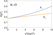
Figure 2: Form factors $F_{1}(q^{2}),F_{0}(q^{2})$ for the $B_{c}\to D$ transition.

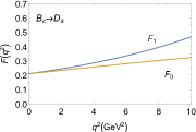
Figure 3: Form factors $F_{1}(q^{2}),F_{0}(q^{2})$ for the $B_{c}\to D_{s}$ transition.

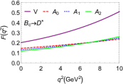
Figure 4: Form factors $V(q^{2})$, $A_{0}(q^{2})$, $A_{1}(q^{2})$ and $A_{2}(q^{2})$ for the $B_{c}\to D^{\ast}$ transition.

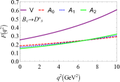
Figure 5: Form factors $V(q^{2})$, $A_{0}(q^{2})$, $A_{1}(q^{2})$ and $A_{2}(q^{2})$ for the $B_{c}\to D^{\ast}_{s}$ transition.

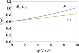
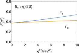
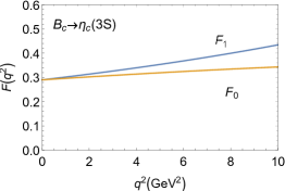
Figure 6: Form factors $F_{1}(q^{2}),F_{0}(q^{2})$ for the $B_{c}\to\eta_{c}$ (left), $B_{c}\to\eta_{c}(2S)$ (center), $B_{c}\to\eta_{c}(3S)$ (right) transitions.

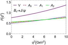
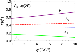
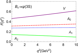
Figure 7: Form factors $V(q^{2})$, $A_{0}(q^{2}),$ $A_{1}(q^{2})$ and $A_{2}(q^{2})$ for the $B_{c}\to J/\Psi$ (left), $B_{c}\to\psi(2S)$ (center) and $B_{c}\to\psi(3S)$ (right) transitions.

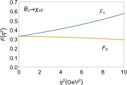
Figure 8: Form factors$F_{1}(q^{2}),F_{0}(q^{2})$ for the $B_{c}\to\chi_{c0}$ transition.

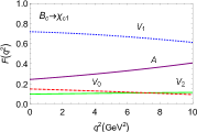
Figure 9: Form factors $A(q^{2}),V_{0}(q^{2}),V_{1}(q^{2})$ and $V_{2}(q^{2})$ for the $B_{c}\to\chi_{c1}$ transition.

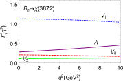
Figure 10: Form factors $A(q^{2})$, $V_{0}(q^{2})$, $V_{1}(q^{2})$ and $V_{2}(q^{2})$ for the $B_{c}\to X(3872)$ transition.

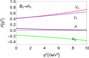
Figure 11: Form factors $A(q^{2})$, $V_{0}(q^{2})$, $V_{1}(q^{2})$ and $V_{2}(q^{2})$ for the $B_{c}\to h_{c}$ transition.

The parameters $a$ and $b$ will be fitted in the space-like region ($-10$ GeV${}^{2}\leq q^{2}\leq 0$). The $q^{2}$-dependence of form factors in the time-like region are plotted in Figs. 3, 3, 5, 5, 6, 7, 9, 9, 11 and 11. In general the slope parameters $a,b$ are very sensitive to the values of $\beta^{\prime}$, while the form factors at $q^{2}=0$ are less sensitive to the variation in $\beta^{\prime}$ values.

III.1 Transition form factors

In Tab. 5, we can find that the values of the $B_{c}\to\eta_{c}$ transition form factors $F^{B_{c}\eta_{c}}_{0,1}$ predicted by many works wwang ; Nobes ; Santorelli ; sun ; Verma ; sharm ; Dhir ; Onishchenko ; P ; Zuo ; T ; Likhoded ; Kiselev are larger than $0.5$, only a few of values D.s ; Galkin ; Hernandez ; Colangelo ; and are less than $0.5$. Similarly, many predictions for the form factor $V^{B_{c}J/\psi}$ are larger than $0.6$ except for a few of values. As for the form factors $A^{B_{c}J/\psi}_{0,1,2}$, most of their values lie in the range of $0.5\sim 0.7$.

In Tab. 6, we compare our results of the $B_{c}\to D,D^{*},D_{s},D_{s}^{*}$ transition form factors at $q^{2}=0$ with other calculations. One can find that our results are consistent with those calculated using the relativistic quark model (RQM) D.s ; Galkin , while they are too large for the results given by the relativistic constituent quark model (RCQM) P , the light-cone sum rule (LCSR) Zuo ; T , and the QCD sum rules Likhoded ; Kiselev . In Refs. Likhoded ; Kiselev , the form factors have a threefold enhancement by including the Coulomb-like $\alpha_{s}/v$ corrections for the heavy quarkonium $B_{c}$. It seems too small for the values of $F^{B_{c}D}_{0,1}$ predicted using the Bauer-Stech-Wirbel (BSW) relativistic quark model Verma . Compared with the previous CLFQM calculations wwang , our predictions for the form factors $V^{B_{c}D^{*}},A^{B_{c}D^{*}}_{0,1,2}$ have a significant enhancement by using a larger decay constant $f_{D^{*}}$, while the influence from the difference values for the decay constant $f_{B_{c}}$ is small.

For the $B_{c}$ transition to a ground-state vector meson, which is either a charmed meson or a charmonium, the form factor $V$ is the largest one, and $A_{0,1,2}$ are close to each other. It is easy to find this character in Figs. 5 and 5 and the first pannel of Fig. 7. On the other hand, if the final-state meson is a radially excited meson $\psi(2S)$ or $\psi(3S)$, the form factors show a hierarchy $V>A_{2}>A_{1}>A_{0}$, which can be found in the last two pannels of Fig.7. Nevertheless, $V$ is always the largest one among the form factors of $B_{c}$ transition to either a ground state or a radially excited charmonium. There also exits another hierarchy for the $B_{c}\to\eta_{c},\eta_{c}(2S),\eta_{c}(3S)$ transitions, $F_{0,1}^{B_{c}\to\eta_{c}}>F_{0,1}^{B_{c}\to\eta_{c}(2S)}>F_{0,1}^{B_{c}\to\eta_{c}(3S)}$. The $q^{2}$ dependence of the $B_{c}\to\chi_{c1}$ transition is shown in Fig.9, where $V_{1}$ is much larger than other form factors $A,V_{0,2}$. It is very like the case of the $B_{c}\to X(3872)$ transition shown in Fig.11. Thus it is a natural assignment of this state as the first radial excitation of a 1P charmonium state $\chi_{c1}$. Because both $\chi_{c1}$ and $X(3872)$ have the same quantum numbers $J^{PC}=1^{++}$, they should have similar properties in $B_{c}$ decays, while it is very different for the $B_{c}$ transition to another type of axial vector meson $h_{c}$ with $J^{PC}=1^{+-}$, where the value of $V_{0}$ is large and close to that of $V_{1}$ as shown in Fig.11. Certainly, the values of the form factor $V_{1}$ for both of $B_{c}$ transitions to these two types of axial vector charmonia are large. By comparing with Fig.11 and 11, one can find that both of the values of $V_{2}$ in the $B_{c}\to X(3873)$ and $B_{c}\to h_{c}$ transition form factors are the smallest; especially, $V_{2}$ for the $B_{c}\to h_{c}$ transition becomes negative. As we know, there is sill no definite answer about the internal properties of the $X(3872)$. From Fig.11, one can find that the form factors of the $B_{c}\to X(3872)$ transition are almost flat in their $q^{2}$ behaviors except for $A^{B_{c}X(3872)}$. A comparison of these values with experimental measurements for the $B_{c}\to X(3872)$ transition form factors will provide unique insight into the mysterious inner structure of $X(3872)$. The form factors for the $B_{c}$ to these P-wave charmonium transitions are listed in Tab. 7.

Table 7: Results for the $B_{c}\to\chi_{c0},\chi_{c1},h_{c},X(3872)$ transition form factors and the fitted parameters $a$ and $b$. The uncertainties are from the decay constants of $B_{c}$ and final state mesons.

F	F(0)	$F(q^{2}_{max})$	a	b
$F^{B_{c}\chi_{c0}}_{1}$	$0.33^{+0.00+0.02}_{-0.02-0.00}$	$0.52^{+0.00+0.04}_{-0.00-0.03}$	$2.07^{+0.02+0.04}_{-0.02-0.04}$	$0.39^{+0.01+0.01}_{-0.01-0.02}$
$F^{B_{c}\chi_{c0}}_{0}$	$0.33^{+0.02+0.02}_{-0.00-0.02}$	$0.30^{+0.02+0.02}_{-0.00-0.02}$	$-0.14^{+0.01+0.06}_{-0.01-0.06}$	$-1.29^{+0.01+0.03}_{-0.01-0.03}$
$A^{B_{c}\chi_{c1}}$	$0.24^{+0.00+0.01}_{-0.00-0.01}$	$0.36^{+0.00+0.02}_{-0.00-0.02}$	$1.96^{+0.02+0.03}_{-0.02-0.03}$	$0.33^{+0.02+0.01}_{-0.01-0.02}$
$V^{B_{c}\chi_{c1}}_{0}$	$0.15^{+0.00+0.00}_{-0.00-0.00}$	$0.11^{+0.00+0.01}_{-0.00-0.00}$	$-1.19^{+0.01+0.20}_{-0.20-0.01}$	$-2.60^{+0.05+0.24}_{-0.05-0.25}$
$V^{B_{c}\chi_{c1}}_{1}$	$0.72^{+0.00+0.02}_{-0.00-0.02}$	$0.65^{+0.00+0.02}_{-0.00-0.03}$	$-0.25^{+0.02+0.10}_{-0.02-0.09}$	$-1.51^{+0.00+0.06}_{-0.00-0.06}$
$V^{B_{c}\chi_{c1}}_{2}$	$0.10^{+0.00+0.00}_{-0.00-0.00}$	$0.11^{+0.00+0.00}_{-0.00-0.00}$	$0.83^{+0.04+0.02}_{-0.03-0.02}$	$-0.77^{+0.05+0.03}_{-0.03-0.05}$
$A^{B_{c}h_{c}}$	$0.06^{+0.00+0.00}_{-0.00-0.00}$	$0.01^{+0.00+0.00}_{-0.00-0.00}$	$-6.24^{+0.08+0.60}_{-0.07-0.66}$	$-14.41^{+0.12+1.46}_{-0.11-1.62}$
$V^{B_{c}h_{c}}_{0}$	$0.41^{+0.03+0.00}_{-0.03-0.00}$	$0.63^{+0.05+0.01}_{-0.05-0.01}$	$2.17^{+0.02+0.05}_{-0.02-0.05}$	$0.38^{+0.01+0.01}_{-0.01-0.02}$
$V^{B_{c}h_{c}}_{1}$	$0.42^{+0.02+0.00}_{-0.02-0.00}$	$0.58^{+0.03+0.01}_{-0.03-0.01}$	$1.64^{+0.02+0.05}_{-0.02-0.0.05}$	$0.22^{+0.00+0.01}_{-0.00-0.01}$
$V^{B_{c}h_{c}}_{2}$	$-0.18^{+0.00+0.01}_{-0.00-0.01}$	$-0.31^{+0.01+0.00}_{-0.00-0.01}$	$2.71^{+0.02+0.04}_{-0.02-0.04}$	$0.61^{+0.01+0.01}_{-0.01-0.02}$
$A^{B_{c}X(3872)}$	$0.28^{+0.00+0.02}_{-0.00-0.03}$	$0.37^{+0.00+0.03}_{-0.00-0.04}$	$1.85^{+0.02+0.09}_{-0.02-0.08}$	$0.38^{+0.01+0.01}_{-0.01-0.03}$
$V^{B_{c}X(3872)}_{0}$	$0.21^{+0.00+0.01}_{-0.00-0.01}$	$0.19^{+0.00+0.02}_{-0.00-0.02}$	$-0.52^{+0.01+0.38}_{-0.01-0.32}$	$-1.45^{+0.02+0.36}_{-0.03-0.32}$
$V^{B_{c}X(3872)}_{1}$	$1.13^{+0.00+0.01}_{-0.00-0.03}$	$1.10^{+0.00+0.05}_{-0.00-0.06}$	$-0.05^{+0.01+0.24}_{-0.01-0.20}$	$-1.03^{+0.00+0.15}_{-0.00-0.12}$
$V^{B_{c}X(3872)}_{2}$	$0.11^{+0.00+0.01}_{-0.01-0.01}$	$0.12^{+0.00+0.01}_{-0.01-0.01}$	$0.77^{+0.03+0.04}_{-0.03-0.04}$	$-0.61^{+0.02+0.08}_{-0.02-0.12}$

Table 8: Comparison of the $B_{c}\to\eta_{c}(2S,3S),\psi(2S,3S),\chi_{c1},h_{c},X(3872)$ transition form factors at $q^{2}=0$ between this work and other literature.

	$F^{B_{c}\eta_{c}(2S)}_{1}(0)=F^{B_{c}\eta_{c}(2S)}_{0}(0)$	$F^{B_{c}\eta_{c}(3S)}_{1}(0)=F^{B_{c}\eta_{c}(3S)}_{0}(0)$	$-$	$-$
This work	$0.37$	$0.29$	$-$	$-$
Rui:2016opu	$1.04$	$0.78$	$-$	$-$
	$V^{B_{c}\psi(2S)}$	$A^{B_{c}\psi(2S)}_{0}$	$A^{B_{c}\psi(2S)}_{1}$	$A^{B_{c}\psi(2S)}_{2}$
This work	$0.57$	$0.41$	$0.35$	$0.17$
Ke13	$0.525$	$0.452$	$0.335$	$0.102$
Rui:2016opu	$1.71$	$0.80$	$0.87$	$1.22$
	$V^{B_{c}\psi(3S)}$	$A^{B_{c}\psi(3S)}_{0}$	$A^{B_{c}\psi(3S)}_{1}$	$A^{B_{c}\psi(3S)}_{2}$
This work	$0.46$	$0.31$	$0.27$	$0.14$
Rui:2016opu	$1.07$	$0.41$	$0.41$	$0.66$
	$A^{B_{c}\chi_{c1}}$	$V^{B_{c}\chi_{c1}}_{0}$	$V^{B_{c}\chi_{c1}}_{1}$	$V^{B_{c}\chi_{c1}}_{2}$
This work	$0.24$	$0.15$	$0.72$	$0.10$
wwang1	$0.36$	$0.13$	$0.85$	$0.15$
	$A^{B_{c}h_{c}}$	$V^{B_{c}h_{c}}_{0}$	$V^{B_{c}h_{c}}_{1}$	$V^{B_{c}h_{c}}_{2}$
This work	$0.06$	$0.41$	$0.42$	$-0.18$
wwang1	$0.07$	$0.64$	$0.50$	$-0.32$
	$A^{B_{c}X(3872)}$	$V^{B_{c}X(3872)}_{0}$	$V^{B_{c}X(3872)}_{1}$	$V^{B_{c}X(3872)}_{2}$
This work	$0.28$	$0.21$	$1.13$	$0.11$
wwang2	$0.36$	$0.18$	$1.15$	$0.13$

From Tab. 8, we can find that the form factors of $B_{c}\to\eta_{c}(2S,3S),\psi(2S,3S)$ transitions calculated in the PQCD approach Rui:2016opu may be more than twice as larger as those predicted in the CLFQM, which will induce large differences for the branching ratios of some correlative decay channels given by these two approaches. In the PQCD appraoch, the form factors are sensitive to the formulae of the $B_{c}$ wave functions. In Ref. Rui:2016opu , the authors argued that the $B_{c}$ wave function in the light-cone formula is broader in shape than that of the traditional zero-point one, which is $\propto\delta(x-r_{c})$, so the overlap between the initial and final states’ wave functions becomes larger by using the light-cone wave function for the $B_{c}$ meson, which induces larger form factors. Our predictions for the $B_{c}$ to vector charmonium $J/\Psi,\psi(2S)$ transition form factors are close to the results given by the LFQM calculations Ke13 except for $A^{B_{c}\psi(2S)}_{2}$. For the $B_{c}$ to the axial vector charmonium transition form factors, our results are also consistent with the previous CLQM calculations wwang1 ; wwang2 .

III.2 Branching ratios

Besides the masses of the constituent quarks and mesons listed in Table. 2, other inputs, such as the $B_{c}$ meson lifetime $\tau_{B_{c}}$, the Wilson coefficients $a_{1},a_{2}$, and the Cabibbo-Kobayashi-Maskawa (CKM) matrix elements, are listed as pdg22 ; buras

$$\tau_{B_{c}} = (0.510\pm 0.009)\times 10^{-12}s,a_{1}=1.07,a_{2}=0.234,$$ (68)

$$V_{cd} = 0.221\pm 0.004,V_{cb}=(40.8\pm 1.4)\times 10^{-3},V_{cs}=0.975\pm 0.006$$ (69)

$$V_{us} = 0.2243\pm 0.0008,V_{ud}=0.97373\pm 0.00031.$$ (70)

First, we consider the branching ratios of the decays $B_{c}\to\eta_{c}(J/\Psi)P(V)$, which can be calculated through the formula

$$\mathcal{B}r(B_{c}\to\eta_{c}(J/\Psi)P(V))=\frac{\tau_{B_{c}}}{\hbar}\Gamma(B_{c}\to\eta_{c}(J/\Psi)P(V)),$$ (71)

where the decay width $\Gamma(B_{c}\to\eta_{c}(J/\Psi)P(V))$ for each channel is given as following

$$\Gamma\left(B_{c}\to\eta_{c}P(V)\right) = \frac{\left|G_{F}V_{cb}V_{uq}^{*}a_{1}f_{P(V)}m_{B_{c}}^{2}F_{0}^{B_{c}\eta_{c}}(m^{2}_{P(V)})\right|^{2}}{32\pi m_{B_{c}}}\left(1-r_{\eta_{c}}^{2}\right),$$ (72)

$$\Gamma\left(B_{c}\to J/\Psi P\right) = \frac{\left|G_{F}V_{cb}V_{uq}^{*}a_{1}f_{P}m_{B_{c}}^{2}A_{0}^{B_{c}J/\Psi}(m^{2}_{P})\right|^{2}}{32\pi m_{B_{c}}}\left(1-r_{J/\psi}^{2}\right),$$ (73)

with the subscript $q=d(s)$ in the CKM element $V_{uq}$ for the decays with $\pi,\rho(K,K^{*})$ involved. For the decays $B_{c}\to J/\Psi V$, the corresponding decay width is the summation of the three polarizations

$$\Gamma\left(B_{c}\to J/\Psi V\right) = \frac{|\vec{p}|}{8\pi m_{B_{c}}^{2}}\left(|\mathcal{A}_{L}(B_{c}\to J/\Psi V)|^{2}+2\left|\mathcal{A}_{N}\left(B_{c}\to J/\Psi V\right)\right|^{2}\right.$$ (74)

$$\left.+2\left|\mathcal{A}_{T}\left(B_{c}\to J/\psi V\right)\right|^{2}\right),$$

where $\vec{p}$ is the three-momentum of either of the two final states in the $B_{c}$ rest frame

$$|\vec{p}|=\frac{\sqrt{\left(m_{B_{c}}^{2}-\left(m_{J/\psi}+m_{V}\right)^{2}\right)\left(m_{B_{c}}^{2}-\left(m_{J/\psi}-m_{V}\right)^{2}\right)}}{2m_{B_{c}}},$$ (75)

and the three polarization amplitudes $\mathcal{A}_{L},\mathcal{A}_{N},and\mathcal{A}_{T}$ are given as

$$\mathcal{A}_{L}\left(B_{c}\to J/\Psi V\right) = \frac{G_{F}}{\sqrt{2}}V^{*}_{cb}V_{uq}a_{1}f_{V}m^{2}_{B_{c}}\frac{1}{2r_{J/\Psi}}\left[\frac{\lambda(1,r^{2}_{J/\Psi},r^{2}_{V})}{1+r_{J/\Psi}}A^{B_{c}J/\Psi}_{2}(m^{2}_{V})\right.$$ (76)

$$\left.-(1-r^{2}_{J/\Psi}-r^{2}_{V})(1+r_{J/\Psi})A^{B_{c}J/\Psi}_{1}(m^{2}_{V})\right],$$

$$\mathcal{A}_{N}\left(B^{+}_{c}\to J/\psi V\right) = -\frac{G_{F}}{\sqrt{2}}V^{*}_{cb}V_{uq}a_{1}f_{V}m_{B_{c}}^{2}r_{V}\left(1+r_{J/\Psi}\right)A_{1}^{B_{c}J/\Psi}\left(m_{V}^{2}\right),$$ (77)

$$\mathcal{A}_{T}\left(B_{c}\to J/\Psi V\right) = -\frac{G_{F}}{\sqrt{2}}V^{*}_{cb}V_{uq}a_{1}f_{V}m_{B_{c}}^{2}r_{V}\frac{\sqrt{\lambda\left(1,r_{J/\Psi}^{2},r_{V}^{2}\right)}}{1+r_{J/\Psi}}V^{B_{c}J/\Psi}\left(m_{V}^{2}\right),$$ (78)

with $\lambda\left(1,r_{J/\Psi}^{2},r_{V}^{2}\right)=\left(1+r_{J/\psi}^{2}-r_{V}^{2}\right)^{2}-4r_{J/\Psi}^{2}$.

Table 9: The CLFQM predictions for branching ratios $(10^{-3})$ of $B_{c}$ decays to final states containing a ground-state S-wave charmonium ($\eta_{c}$ or $J/\Psi$) and a light pseudoscalar or vector meson. The first error is induced by the $B_{c}$ meson life time, and the second and third uncertainties are from the decay constants of $B_{c}$ and charmonia.

mode	This work	Qiao	Ebert	chang	V	Ivanov	Naimuddin	Colangelo1	Abd	Rui:2014tpa	Rui:2016opu	wwang2	Ke13
$B^{+}_{c}\to J/\psi\pi^{+}$	$1.97^{+0.04+0.00+0.24}_{-0.04-0.00-0.25}$	$2.91(2.22)$	$0.61$	$2.1$	$1.3$	$1.7$	$0.34$	$1.3$	$1.1$	$2.33$	$2.6$	$2.0$	$0.664$
$B^{+}_{c}\to J/\psi K^{+}$	$0.16^{+0.00+0.00+0.02}_{-0.00-0.00-0.02}$	$0.22(0.16)$	$0.05$	$0.16$	$0.11$	$0.13$	$0.11$	$0.07$	$0.08$	$0.19$	$-$	$0.16$	$0.0527$
$B^{+}_{c}\to J/\psi\rho^{+}$	$5.34^{+0.09+0.07+0.73}_{-0.09-0.07-0.63}$	$8.08(6.03)$	$1.6$	$6.5$	$4.0$	$4.9$	$1.8$	$3.7$	$3.1$	$8.20$	$-$	$5.0$	$-$
$B^{+}_{c}\to J/\psi K^{*+}$	$0.31^{+0.01+0.00+0.04}_{-0.01-0.00-0.04}$	$0.43(0.32)$	$0.10$	$0.35$	$0.22$	$0.28$	$0.09$	$0.2$	$0.18$	$0.48$	$-$	$0.29$	$0.109$
$B^{+}_{c}\to\eta_{c}\pi^{+}$	$2.36^{+0.04+0.00+0.06}_{-0.04-0.00-0.06}$	$5.19(2.95)$	$0.85$	$2.2$	$2.0$	$1.9$	$0.34$	$0.26$	$1.4$	$2.98$	$5.2$	$-$	$-$
$B^{+}_{c}\to\eta_{c}K^{+}$	$0.19^{+0.00+0.00+0.00}_{-0.00-0.00-0.01}$	$0.38(0.21)$	$0.07$	$0.17$	$0.13$	$0.15$	$0.03$	$0.02$	$0.11$	$0.24$	$-$	$-$	$-$
$B^{+}_{c}\to\eta_{c}\rho^{+}$	$6.01^{+0.11+0.00+0.16}_{-0.11-0.01-0.16}$	$14.5(7.89)$	$2.1$	$5.9$	$4.2$	$4.5$	$1.06$	$0.67$	$3.3$	$9.83$	$-$	$-$	$-$
$B^{+}_{c}\to\eta_{c}K^{*+}$	$0.34^{+0.01+0.00+0.01}_{-0.01-0.00-0.01}$	$0.77(0.41)$	$0.11$	$0.31$	$0.20$	$0.25$	$0.06$	$0.04$	$0.18$	$0.57$	$-$	$-$	$-$

From Tab. 9, one can find that our predictions are consistent with the results given by the QCD sum rules V , the relativistic constituent quark model (RCQM) Ivanov and the Bethe-Salpeter equation approach under the so-called instantaneous nonrelativistic approximation chang . In Ref. Qiao , the authors calculated these decays in the nonrelativistic QCD (NRQCD) approach at the next-to-leading-order (NLO) in the QCD coupling $\alpha_{s}$. It is interesting that the leading-order (LO) results for these channels, except for the decay $B^{+}_{c}\to J/\Psi\rho^{+}$ are in agreement with our predictions, while the branching ratios obtain substantial enhancement after including the NLO QCD correction, which provides a large factor $K$. We wonder whether these results will still be stable with the higher order corrections, such as the next-to-next-to-leading-order (NNLO) contributions, involved. In Ref. Ebert , the branching ratios are calculated in the relativistic quark model using $v/c$ expansion for $B_{c}$ and the charmonium, and the obtained results are smaller than most of other predictions, including ours; for example, their results are only about one third of our predictions in most cases. Certainly, the results given in the QCD relativistic (potential) models Colangelo1 ; Abd are also small. As mentioned earlier, the results calculated using the PQCD approach are sensitive to the types of wave functions for $B_{c}$ meson (the traditional zero-point wave function and the light-cone wave function). For example, if taking the light-cone wave function for the $B_{c}$ meson, the branching ratio of the decay $B^{+}_{c}\to\eta_{c}\pi^{+}$ will reach $(5.2^{+2.6}_{-1.4})\times 10^{-3}$ Rui:2016opu , which is much larger than $(2.98^{+1.24}_{-1.05})\times 10^{-3}$ obtained using the traditional zero-point one. From Tab. 9, one can find that the ratio of the branching fractions $R_{K/\pi}\equiv\frac{Br(B_{c}^{+}\to J/\Psi K^{+})}{Br(B_{c}^{+}\to J/\Psi\pi^{+})}=0.081\pm 0.011$, which is consistent with the value $R_{K/\pi}=0.079\pm 0.007\pm 0.003$ given by the LHCb collaboration lhcb1 .

If replacing $P(V)$ with $D(D^{*})$, the branching ratios of the corresponding decays $B_{c}\to\eta_{c}(J/\Psi)D(D^{*})$ can be obtained by their decay widths:

$$\Gamma\left(B_{c}\to\eta_{c}D\right) = \frac{\left(G_{F}V^{*}_{cb}V_{cd}m_{B_{c}}^{2}\right)^{2}\left(1-r_{\eta_{c}}^{2}-r_{D}^{2}\right)}{32\pi m_{B_{c}}}$$ (79)

$$\times|a_{1}f_{D}F_{0}^{B_{c}\eta_{c}}(m_{D}^{2})+a_{2}f_{\eta_{c}}F_{0}^{B_{c}D}(m_{\eta_{c}}^{2})|^{2},$$

$$\Gamma\left(B_{c}\to\eta_{c}D^{\ast}\right) = \frac{\left(G_{F}V^{*}_{cb}V_{cd}m_{B_{c}}^{2}\right)^{2}\left(1-r_{\eta_{c}}^{2}-r_{D^{\ast}}^{2}\right)}{32\pi m_{B_{c}}}$$ (80)

$$\times|a_{1}f_{D^{\ast}}F_{0}^{B_{c}\eta_{c}}(m_{D^{*}}^{2})+a_{2}f_{\eta_{c}}A_{0}^{B_{c}D^{\ast}}(m_{\eta_{c}}^{2})|^{2},$$

$$\Gamma\left(B_{c}\to J/\Psi D\right) = \frac{\left(G_{F}V^{*}_{cb}V_{cd}m_{B_{c}}^{2}\right)^{2}\left(1-r_{J/\psi}^{2}-r_{D}^{2}\right)}{32\pi m_{B_{c}}}$$ (81)

$$\times|a_{1}f_{D}A_{0}^{B_{c}J/\Psi}(m^{2}_{D})+a_{2}f_{J/\Psi}F_{0}^{B_{c}D}(m^{2}_{J/\Psi})|^{2}.$$

For the decay $B_{c}\to J/\Psi D^{*}$, the corresponding decay width is the summation of the three polarizations:

$$\Gamma\left(B_{c}\to J/\Psi D^{*}\right) = \frac{|\vec{p}|}{8\pi m_{B_{c}}^{2}}\left(|\mathcal{A}_{L}(B_{c}\to J/\Psi D^{*})|^{2}+2\left|\mathcal{A}_{N}\left(B_{c}\to J/\Psi D^{*}\right)\right|^{2}\right.$$ (82)

$$\left.+2\left|\mathcal{A}_{T}\left(B_{c}\to J/\Psi D^{*}\right)\right|^{2}\right),$$

where the three polarization amplitudes $\mathcal{A}_{L},\mathcal{A}_{N}$ and $\mathcal{A}_{T}$ are given as

$$\mathcal{A}_{L}\left(B_{c}\to J/\Psi D^{\ast}\right) = \frac{G_{F}}{\sqrt{2}}V^{*}_{cb}V_{cd}m^{2}_{B_{c}}\left\{-(1-r^{2}_{J/\Psi}-r^{2}_{D^{*}})\right.$$

$$\left.\times\left[\frac{a_{1}f_{D^{*}}(1+r_{J/\Psi})}{2r_{J/\Psi}}A^{B_{c}J/\Psi}_{1}(m^{2}_{D^{*}})+\frac{a_{2}f_{J/\Psi}(1+r_{D^{*}})}{2r_{D^{*}}}A^{B_{c}D^{*}}_{1}(m^{2}_{J/\Psi})\right]\right.$$

$$\left.+\frac{a_{1}\lambda_{1}f_{D^{*}}}{2r_{J/\Psi}(1+r_{J/\Psi})}A^{B_{c}J/\Psi}_{2}(m^{2}_{D^{*}})+\frac{a_{2}\lambda_{2}f_{J/\Psi}}{2r_{D^{*}}(1+r_{D^{*}})}A^{B_{c}D^{*}}_{2}(m^{2}_{J/\Psi})\right\},$$

$$\mathcal{A}_{N}\left(B_{c}\rightarrow J/\psi D^{\ast}\right) = -\frac{G_{F}}{\sqrt{2}}V^{*}_{cb}V_{cd}m_{B_{c}}^{2}[a_{1}f_{D^{\ast}}r_{D^{\ast}}\left(1+r_{J/\Psi}\right)A_{1}^{B_{c}J/\Psi}\left(m_{D^{\ast}}^{2}\right)$$ (84)

$$+a_{2}f_{J/\Psi}r_{J/\Psi}\left(1+r_{D^{\ast}}\right)A_{1}^{B_{c}D^{\ast}}\left(m_{J/\Psi}^{2}\right)],$$

$$\mathcal{A}_{T}\left(B_{c}\to J/\Psi D^{\ast}\right) = -\frac{G_{F}}{\sqrt{2}}V^{*}_{cb}V_{cd}m_{B_{c}}^{2}\left[\frac{a_{1}\sqrt{\lambda_{1}}}{1+r_{J/\Psi}}f_{D^{\ast}}r_{D^{\ast}}V^{B_{c}J/\Psi}\left(m_{D^{\ast}}^{2}\right)\right.$$ (85)

$$\left.+\frac{a_{2}\sqrt{\lambda_{2}}}{1+r_{D^{\ast}}}f_{J/\Psi}r_{J/\Psi}V^{B_{c}D^{\ast}}\left(m_{J/\psi}^{2}\right)\right],$$

with $\lambda_{1}=\lambda\left(1,r_{J/\Psi}^{2},r_{D^{\ast}}^{2}\right),\lambda_{2}=\lambda\left(1,r_{D^{\ast}}^{2},r_{J/\Psi}^{2}\right)$. As for the decay widths of the decays $B_{c}\to\eta_{c}(J/\Psi)D_{s}(D^{*}_{s})$, they can be obtained by performing the replacements $D\rightarrow D_{s},D^{*}\rightarrow D^{*}_{s},V_{cd}\rightarrow V_{cs}$ in Eqs.(79)$-$(85). The calculation results are listed in Tab. 10. One can find that our predictions are a little larger than most of other results, but are smaller the the PQCD calculations. The branching ratios of the decays with $D^{(*)}_{s}$ involved are at least one order larger than those of the corresponding decays with $D^{(*)}$ involved. This is because the CKM matrix element $V_{cs}$ associated with the former is much larger than $V_{cd}$ associated with the latter. All of these decays with the ground-state S-wave charmonia involved have large branching ratios, which lie in the range of $10^{-4}\sim 10^{-3}$ and can be detected by the present LHCb experiments. In Ref. aajj3 , if assuming that the spectator diagram dominates and that factorization holds, one can obtain the approximations

$$R_{D^{+}_{s}/\pi^{+}} \equiv \frac{\Gamma(B^{+}_{c}\to J/\Psi D^{+}_{s})}{\Gamma(B^{+}_{c}\to J/\Psi\pi^{+})}\approx\frac{\Gamma(B^{+}_{c}\to\bar{D}^{*}D^{+}_{s})}{\Gamma(B^{+}_{c}\to\bar{D}^{*}\pi^{+})},$$ (86)

$$R_{D^{*+}_{s}/D^{+}_{s}} \equiv \frac{\Gamma(B^{+}_{c}\to J/\Psi D^{*+}_{s})}{\Gamma(B^{+}_{c}\to J/\Psi D^{+}_{s})}\approx\frac{\Gamma(B^{+}_{c}\to\bar{D}^{*}D^{*+}_{s})}{\Gamma(B^{+}_{c}\to\bar{D}^{*}D^{+}_{s})},$$ (87)

which were measured as $R_{D^{+}_{s}/\pi^{+}}=2.90\pm 0.57\pm 0.24$ and $R_{D^{*+}_{s}/D^{+}_{s}}=2.37\pm 0.56\pm 0.10$ by the LHCb collaboration aajj3 , and given as $R_{D^{+}_{s}/\pi^{+}}=2.76\pm 0.47$ and $R_{D^{*+}_{s}/D^{+}_{s}}=1.93\pm 0.26$ by ATLAS atlas . From our calculations, these two ratios are obtained as

$$R_{D^{+}_{s}/\pi^{+}} \equiv \frac{\Gamma(B^{+}_{c}\to J/\Psi D^{+}_{s})}{\Gamma(B^{+}_{c}\to J/\Psi\pi^{+})}=3.09\pm 1.05,$$ (88)

$$R_{D^{*+}_{s}/D^{+}_{s}} \equiv \frac{\Gamma(B^{+}_{c}\to J/\Psi D^{*+}_{s})}{\Gamma(B^{+}_{c}\to J/\Psi D^{+}_{s})}=1.48\pm 0.50,$$ (89)

where the value of $R_{D^{+}_{s}/\pi^{+}}$ is consistent with the measurements given by LHCb and ATLAS, while $R_{D^{*+}_{s}/D^{+}_{s}}$ can explain the ATLAS result within errors.

Table 10: CLFQM predictions for branching ratios $(10^{-3})$ of $B_{c}$ decays to final states containing a ground-state S-wave charmonium ($\eta_{c}$ or $J/\Psi$) and a charmed meson. The errors are induced by the same sources as in Table 9.

mode	This work	chang	V	Ivanov	Naimuddin	Colangelo	Abd	FU	Rui:2014tpa
$B^{+}_{c}\to\eta_{c}D^{+}$	$0.22^{+0.00+0.01+0.02}_{-0.00-0.01-0.00}$	$0.012$	$0.15$	$0.19$	$0.06$	$0.05$	$0.14$	$0.10$	$0.44$
$B^{+}_{c}\to J/\psi D^{+}$	$0.20^{+0.00+0.00+0.03}_{-0.00-0.00-0.03}$	$0.009$	$0.09$	$0.15$	$0.04$	$0.13$	$0.09$	$0.09$	$0.28$
$B^{+}_{c}\to\eta_{c}D^{*+}$	$0.31^{+0.01+0.00+0.01}_{-0.01-0.00-0.01}$	$0.010$	$0.10$	$0.19$	$0.07$	$0.02$	$0.13$	$0.10$	$0.58$
$B^{+}_{c}\to J/\psi D^{*+}$	$0.41^{+0.01+0.00+0.05}_{-0.01-0.00-0.01}$	$-$	$0.28$	$0.45$	$0.18$	$0.19$	$0.28$	$0.28$	$0.67$
$B^{+}_{c}\to\eta_{c}D^{+}_{s}$	$6.44^{+0.11+0.73+0.94}_{-0.11-0.71-0.50}$	$0.54$	$2.8$	$4.4$	$1.79$	$5$	$2.6$	$2.5$	$12.32$
$B^{+}_{c}\to J/\psi D^{+}_{s}$	$6.09^{+0.11+0.36+1.15}_{-0.11-0.33-0.47}$	$0.41$	$1.7$	$3.4$	$1.15$	$3.4$	$1.5$	$2.2$	$8.05$
$B^{+}_{c}\to\eta_{c}D^{*+}_{s}$	$6.97^{+0.12+0.17+0.39}_{-0.12-0.14-0.07}$	$0.44$	$2.7$	$3.7$	$1.49$	$0.38$	$2.4$	$2.0$	$16.54$
$B^{+}_{c}\to J/\psi D^{*+}_{s}$	$9.03^{+0.04+0.02+0.34}_{-0.04-0.02-0.32}$	$-$	$6.7$	$9.7$	$4.4$	$5.9$	$5.5$	$6.0$	$20.45$

Next, we consider the decays with the P-wave charmonia involved in the final states. The P-wave charmonium can be $\chi_{c0},\chi_{c1}$ or $h_{c}$. The decay widths of the decays $B_{c}\to\chi_{c0(1)}P(V),h_{c}P(V)$ are given as follows

$$\Gamma\left(B_{c}\to\chi_{c0}P(V)\right) = \frac{\left|G_{F}V_{cb}V_{uq}^{*}a_{1}f_{P(V)}m_{B_{c}}^{2}F_{0}^{B_{c}\chi_{c0}}(m^{2}_{P(V)})\right|^{2}}{32\pi m_{B_{c}}}\left(1-r_{\chi_{c0}}^{2}\right),$$ (90)

$$\Gamma\left(B_{c}\to\chi_{c1}P\right) = \frac{\left|G_{F}V_{cb}V_{uq}^{*}a_{1}f_{P}m_{B_{c}}^{2}A_{0}^{B_{c}\chi_{c1}}(m^{2}_{P})\right|^{2}}{32\pi m_{B_{c}}}\left(1-r_{\chi_{c1}}^{2}\right),$$ (91)

where the subscript $q=d(s)$ in the CKM element $V_{uq}$ for the decays with $\pi,\rho(K,K^{*})$ involved. For the decays $B_{c}\to\chi_{c1}V$, the corresponding decay widths are the summation of the three polarizations

$$\Gamma\left(B_{c}\to\chi_{c1}V\right) = \frac{|\vec{p}|}{8\pi m_{B_{c}}^{2}}\left(|\mathcal{A}_{L}(B_{c}\to\chi_{c1}V)|^{2}+2\left|\mathcal{A}_{N}\left(B_{c}\to\chi_{c1}V\right)\right|^{2}\right.$$ (92)

$$\left.+2\left|\mathcal{A}_{T}\left(B_{c}\to\chi_{c1}V\right)\right|^{2}\right),$$

where

$$\mathcal{A}_{L}\left(B_{c}\to\chi_{c1}V\right) = \frac{G_{F}}{\sqrt{2}}V^{*}_{cb}V_{uq}a_{1}f_{V}m^{2}_{B_{c}}\frac{1}{2r_{\chi_{c1}}}\left[\frac{\lambda(1,r^{2}_{\chi_{c1}},r^{2}_{V})}{1-r_{\chi_{c1}}}V^{B_{c}\chi_{c1}}_{2}(m^{2}_{V})\right.$$ (93)

$$\left.-(1-r^{2}_{\chi_{c1}}-r^{2}_{V})(1-r_{\chi_{c1}})V^{B_{c}\chi_{c1}}_{1}(m^{2}_{V})\right],$$

$$\mathcal{A}_{N}\left(B^{+}_{c}\to\chi_{c1}V\right) = -\frac{G_{F}}{\sqrt{2}}V^{*}_{cb}V_{uq}a_{1}f_{V}m_{B_{c}}^{2}r_{V}\left(1-r_{\chi_{c1}}\right)V_{1}^{B_{c}\chi_{c1}}\left(m_{V}^{2}\right),$$ (94)

$$\mathcal{A}_{T}\left(B_{c}\to\chi_{c1}V\right) = -\frac{G_{F}}{\sqrt{2}}V^{*}_{cb}V_{uq}a_{1}f_{V}m_{B_{c}}^{2}r_{V}\frac{\sqrt{\lambda\left(1,r_{\chi_{c1}}^{2},r_{V}^{2}\right)}}{1-r_{\chi_{c1}}}A^{B_{c}\chi_{c1}}\left(m_{V}^{2}\right).$$ (95)

It is noted that the analytic formulae of the decay widths between the decays $B_{c}\to h_{c}P(V)$ and $B_{c}\to\chi_{1c}P(V)$ are similar. Summing the branching fractions of the these decays in Tab. 11, we find that the results of the decays with $\pi^{+}(\rho^{+})$ involved are about one order of magnitude larger compared with those of the decays with $K^{+}(K^{*+})$ involved. The difference mainly comes from the the CKM matrix elements: the former involve a larger factor $V_{ud}\sim 1$, while the latter is associated with a smaller factor $V_{us}=\lambda\sim 0.225$. Our predictions are comparable to most other theoretical results, such as the QCD-motivated RQM based on the quasi-potential approach R.N , the NRQM Hernandez , the RCQM M.A . The branching ratios of the decays $B_{c}\to\chi_{c0(1)}P(V)$ predicted by most works have a common property: $Br(B_{c}\to\chi_{c0}P(V))$ are much larger than $Br(B_{c}\to\chi_{c1}P(V))$. This characteristic can be tested by the present LHCb experiments.

Table 11: The CLFQM predictions for branching ratios $(10^{-3})$ of $B_{c}$ decays to final states containing a P-wave charmonium and a light pseudoscalar or vector meson. The errors are induced by the same sources as in Table 9.

mode	This work	R.N	Hernandez	M.A	Zong	O.N	Z.H	Zhu	Rui:2017pre
$B^{+}_{c}\to\chi_{c0}\pi^{+}$	$0.66^{+0.01+0.01+0.08}_{-0.01-0.01-0.07}$	$0.21$	$0.26$	$0.55$	$0.28$	$9.8$	$0.31$	$4.2$	$1.6$
$B^{+}_{c}\to\chi_{c1}\pi^{+}$	$0.13^{+0.00+0.00+0.00}_{-0.00-0.00-0.00}$	$0.2$	$0.0014$	$0.068$	$0.07$	$0.089$	$0.021$	$0.05$	$0.51$
$B^{+}_{c}\to h_{c}\pi^{+}$	$0.96^{+0.02+0.02+0.13}_{-0.02-0.02-0.12}$	$0.46$	$0.53$	$1.1$	$0.5$	$16$	$0.98$	$6.2$	$0.54$
$B^{+}_{c}\to\chi_{c0}\rho^{+}$	$1.69^{+0.00+0.02+0.20}_{-0.00-0.02-0.19}$	$0.58$	$0.67$	$1.3$	$0.72$	$33$	$0.76$	$-$	$5.8$
$B^{+}_{c}\to\chi_{c1}\rho^{+}$	$0.43^{+0.01+0.00+0.01}_{-0.01-0.00-0.01}$	$0.15$	$0.1$	$0.29$	$0.29$	$4.6$	$0.23$	$1.47$	$2.8$
$B^{+}_{c}\to h_{c}\rho^{+}$	$2.42^{+0.04+0.16+0.19}_{-0.04-0.09-0.42}$	$1.0$	$1.3$	$2.5$	$1.2$	$53$	$2.2$	$1.24$	$2.3$
$B^{+}_{c}\to\chi_{c0}K^{+}$	$0.052^{+0.001+0.001+0.006}_{-0.001-0.001-0.006}$	$0.016$	$0.02$	$0.042$	$0.0021$	$-$	$0.023$	$0.32$	$0.12$
$B^{+}_{c}\to\chi_{c1}K^{+}$	$0.010^{+0.000+0.000+0.000}_{-0.000-0.000-0.000}$	$0.015$	$0.00011$	$0.0051$	$0.00052$	$-$	$0.0016$	$0.004$	$0.038$
$B^{+}_{c}\to h_{c}K^{+}$	$0.075^{+0.001+0.001+0.010}_{-0.001-0.001-0.001}$	$0.035$	$0.041$	$0.083$	$0.0038$	$-$	$0.074$	$0.47$	$0.043$
$B^{+}_{c}\to\chi_{c0}K^{*+}$	$0.096^{+0.002+0.001+0.011}_{-0.002-0.001-0.011}$	$0.04$	$0.037$	$0.07$	$0.0039$	$-$	$0.045$	$-$	$0.33$
$B^{+}_{c}\to\chi_{c1}K^{*+}$	$0.027^{+0.001+0.000+0.000}_{-0.001-0.000-0.000}$	$0.01$	$0.0073$	$0.018$	$0.0018$	$-$	$0.017$	$0.0707$	$0.18$
$B^{+}_{c}\to h_{c}K^{*+}$	$0.13^{+0.00+0.00+0.02}_{-0.00-0.01-0.01}$	$0.07$	$0.071$	$0.13$	$0.0068$	$-$	$0.13$	$0.0618$	$0.13$

If replacing $P(V)$ with $D(D^{*})$ in the upper decays, the branching ratios of the corresponding decays $B_{c}\to\chi_{c0(1)}(h_{c})D(D^{*})$ can be obtained by their decay widths:

$$\Gamma\left(B_{c}\to\chi_{c0}D\right) = \frac{\left(G_{F}V^{*}_{cb}V_{cd}m_{B_{c}}^{2}\right)^{2}\left(1-r_{\chi_{c0}}^{2}-r_{D}^{2}\right)}{32\pi m_{B_{c}}}$$ (96)

$$\times|a_{1}f_{D}F_{0}^{B_{c}\chi_{c0}}(m_{D}^{2})+a_{2}f_{\chi_{c0}}F_{0}^{B_{c}D}(m_{\chi_{c0}}^{2})|^{2},$$

$$\Gamma\left(B_{c}\to\chi_{c0}D^{\ast}\right) = \frac{\left(G_{F}V^{*}_{cb}V_{cd}m_{B_{c}}^{2}\right)^{2}\left(1-r_{\chi_{c0}}^{2}-r_{D^{\ast}}^{2}\right)}{32\pi m_{B_{c}}}$$ (97)

$$\times|a_{1}f_{D^{\ast}}F_{0}^{B_{c}\chi_{c0}}(m_{D^{*}}^{2})+a_{2}f_{\chi_{c0}}A_{0}^{B_{c}D^{\ast}}(m_{\chi_{c0}}^{2})|^{2},$$

$$\Gamma\left(B_{c}\to\chi_{c1}D\right) = \frac{\left(G_{F}V^{*}_{cb}V_{cd}m_{B_{c}}^{2}\right)^{2}\left(1-r_{\chi_{c1}}^{2}-r_{D}^{2}\right)}{32\pi m_{B_{c}}}$$ (98)

$$\times|a_{1}f_{D}V_{0}^{B_{c}\chi_{c1}}(m_{D}^{2})+a_{2}f_{\chi_{c1}}F_{0}^{B_{c}D}(m_{\chi_{c1}}^{2})|^{2}.$$

Table 12: CLFQM predictions for branching ratios $(10^{-3})$ of $B_{c}$ decays to final states containing a P-wave charmonium ($\chi_{c0},\chi_{c1}$ or $h_{c}$) and a light pseudoscalar or vector meson. The errors are induced by the same sources as in Table 9.

mode	This work	hffu
$B^{+}_{c}\to\chi_{c0}D^{+}$	$0.075^{+0.001+0.001+0.001}_{-0.001-0.001-0.001}$	$0.033$
$B^{+}_{c}\to\chi_{c1}D^{+}$	$0.019^{+0.000+0.000+0.001}_{-0.000-0.000-0.001}$	$0.14\times 10^{-3}$
$B^{+}_{c}\to h_{c}D^{+}$	$0.075^{+0.001+0.001+0.011}_{-0.001-0.001-0.010}$	$0.066$
$B^{+}_{c}\to\chi_{c0}D^{+}_{s}$	$2.29^{+0.04+0.02+0.34}_{-0.04-0.07-0.23}$	$0.88$
$B^{+}_{c}\to\chi_{c1}D^{+}_{s}$	$0.60^{+0.01+0.03+0.06}_{-0.01-0.04-0.01}$	$0.20\times 10^{-2}$
$B^{+}_{c}\to h_{c}D^{+}_{s}$	$2.24^{+0.04+0.02+0.33}_{-0.04-0.04-0.29}$	$1.58$
$B^{+}_{c}\to\chi_{c0}D^{*+}$	$0.11^{+0.00+0.00+0.01}_{-0.00-0.00-0.01}$	$0.042$
$B^{+}_{c}\to\chi_{c1}D^{*+}$	$0.054^{+0.001+0.000+0.000}_{-0.001-0.000-0.000}$	$0.026$
$B^{+}_{c}\to h_{c}D^{*+}$	$0.11^{+0.00+0.00+0.03}_{-0.00-0.00-0.01}$	$0.071$
$B^{+}_{c}\to\chi_{c0}D^{*+}_{s}$	$2.49^{+0.04+0.02+0.32}_{-0.04-0.33-0.30}$	$0.84$
$B^{+}_{c}\to\chi_{c1}D^{*+}_{s}$	$1.23^{+0.02+0.00+0.07}_{-0.02-0.01-0.07}$	$0.49$
$B^{+}_{c}\to h_{c}D^{*+}_{s}$	$2.41^{+0.04+0.02+0.34}_{-0.04-0.02-0.32}$	$1.34$

For the decay $B_{c}\to\chi_{c1}D^{*}$, the corresponding decay width is the summation of the three polarizations:

$$\Gamma\left(B_{c}\to\chi_{c1}D^{*}\right) = \frac{|\vec{p}|}{8\pi m_{B_{c}}^{2}}\left(|\mathcal{A}_{L}(B_{c}\to\chi_{c1}D^{*})|^{2}+2\left|\mathcal{A}_{N}\left(B_{c}\to\chi_{c1}D^{*}\right)\right|^{2}\right.$$ (99)

$$\left.+2\left|\mathcal{A}_{T}\left(B_{c}\to\chi_{c1}D^{*}\right)\right|^{2}\right),$$

where the three polarization amplitudes $\mathcal{A}_{L},\mathcal{A}_{N}$ and $\mathcal{A}_{T}$ are given as

$$\mathcal{A}_{L}\left(B_{c}\to\chi_{c1}D^{\ast}\right) = \frac{G_{F}}{\sqrt{2}}V^{*}_{cb}V_{cd}m^{2}_{B_{c}}\left\{-(1-r^{2}_{\chi_{c1}}-r^{2}_{D^{*}})\right.$$ (100)

$$\left.\times\left[\frac{a_{1}f_{D^{*}}(1-r_{\chi_{c1}})}{2r_{\chi_{c1}}}V^{B_{c}\chi_{c1}}_{1}(m^{2}_{D^{*}})+\frac{a_{2}f_{\chi_{c1}}(1+r_{D^{*}})}{2r_{D^{*}}}A^{B_{c}D^{*}}_{1}(m^{2}_{\chi_{c1}})\right]\right.$$

$$\left.+\frac{a_{1}\lambda_{1}f_{D^{*}}}{2r_{\chi_{c1}}(1-r_{\chi_{c1}})}V^{B_{c}\chi_{c1}}_{2}(m^{2}_{D^{*}})+\frac{a_{2}\lambda_{2}f_{\chi_{c1}}}{2r_{D^{*}}(1+r_{D^{*}})}A^{B_{c}D^{*}}_{2}(m^{2}_{\chi_{c1}})\right\},\;\;\;$$

$$\mathcal{A}_{N}\left(B_{c}\to\chi_{c1}D^{\ast}\right) = -\frac{G_{F}}{\sqrt{2}}V^{*}_{cb}V_{cd}m_{B_{c}}^{2}[a_{1}f_{D^{\ast}}r_{D^{\ast}}\left(1-r_{\chi_{c1}}\right)V_{1}^{B_{c}\chi_{c1}}\left(m_{D^{\ast}}^{2}\right)$$ (101)

$$+a_{2}f_{\chi_{c1}}r_{\chi_{c1}}\left(1+r_{D^{\ast}}\right)A_{1}^{B_{c}D^{\ast}}\left(m_{\chi_{c1}}^{2}\right)],$$

$$\mathcal{A}_{T}\left(B_{c}\to\chi_{c1}D^{\ast}\right) = -\frac{G_{F}}{\sqrt{2}}V^{*}_{cb}V_{cd}m_{B_{c}}^{2}\left[\frac{a_{1}\sqrt{\lambda_{1}}}{1-r_{\chi_{c1}}}f_{D^{\ast}}r_{D^{\ast}}A^{B_{c}\chi_{c1}}\left(m_{D^{\ast}}^{2}\right)\right.$$ (102)

$$\left.+\frac{a_{2}\sqrt{\lambda_{2}}}{1+r_{D^{\ast}}}f_{\chi_{c1}}r_{\chi_{c1}}V^{B_{c}D^{\ast}}\left(m_{\chi_{c1}}^{2}\right)\right],$$

with $\lambda_{1}=\lambda\left(1,r_{\chi_{c1}}^{2},r_{D^{\ast}}^{2}\right),\lambda_{2}=\lambda\left(1,r_{D^{\ast}}^{2},r_{\chi_{c1}}^{2}\right)$. As to the decay widths of the channels $B_{c}\to\chi_{c0}(\chi_{c1})D_{s}(D^{*}_{s})$, they can be obtained by performing the replacements $D\to D_{s},D^{*}\rightarrow D^{*}_{s},V_{cd}\rightarrow V_{cs}$ in Eqs. (96)$-$(102). The branching ratios of the these decays are given in Tab. 12, where we also list the results given by the Salpeter method hffu . This method is the relativistic instantaneous approximation of the original Bethe-Salpeter equation.

Table 13: CLFQM predictions for branching ratios $(\times 10^{-3})$ of the decays $B_{c}\to X(3872)M$, where $M$ represents a light pseudoscalar, a vector meson, or a charmed meson. The errors are induced by the same sources as in Table 9.

mode	This work	wwang2	Zhang:2022xqs	Hsiao:2016pml
$B^{+}_{c}\to X(3872)\pi^{+}$	$0.25^{+0.00+0.01+0.03}_{-0.00-0.01-0.01}$	$0.17$	$0.27$	$0.06$
$B^{+}_{c}\to X(3872)K^{+}$	$0.020^{+0.000+0.001+0.000}_{-0.000-0.001-0.000}$	$0.013$	$0.025$	$0.0047$
$B^{+}_{c}\to X(3872)\rho^{+}$	$0.63^{+0.01+0.03+0.03}_{-0.01-0.03-0.08}$	$0.41$	$-$	$-$
$B^{+}_{c}\to X(3872)K^{*+}$	$0.036^{+0.001+0.001+0.004}_{-0.001-0.002-0.002}$	$0.024$	$-$	$-$
$B^{+}_{c}\to X(3872)D^{+}$	$0.033^{+0.001+0.002+0.001}_{-0.001-0.002-0.000}$	$-$
$B^{+}_{c}\to X(3872)D^{*+}$	$0.078^{+0.001+0.007+0.009}_{-0.001-0.007-0.006}$	$-$
$B^{+}_{c}\to X(3872)D^{+}_{s}$	$1.00^{+0.02+0.15+0.15}_{-0.02-0.15-0.10}$	$-$
$B^{+}_{c}\to X(3872)D^{*+}_{s}$	$1.78^{+0.03+0.07+0.12}_{-0.03-0.07-0.08}$	$-$

Though the $X(3872)$ has been confirmed by many experimental collaborations, such as CDF cdf , D0 d0 , Babar babar0 and LHCb lhcb , with quantum numbers $J^{PC}=1^{++}$ and isospin $I=0$, there are still many uncertainties. Though many different exotic hadron state interpretations, such as a loosely bound molecular state close ; wong ; braaten0 ; swanson ; zhusl , a compact tetraquark state chiu ; barnea ; maiani1 ; hogaasen , $c\bar{c}g$ hybrid meson close2 ; li , glueball li , have been put forward, the first raidal excitation of $1P$ charmonium state $\chi_{c1}(1P)$ as the most natural assignment has not been ruled out barnes ; eichten ; quigg . By assuming the $X(3872)$ as a $1^{++}$ charmonium state, we calculate the branching ratios of the decays $B^{+}_{c}\to X(3872)M$ (here, $M$ represents a light pseudoscalar, a vector meson, or a charmed meson). The analytic expressions of the corresponding decay widths are similar to those of the decays $B_{c}\to\chi_{c1}M$ listed in Eqs. (91), (92), (98) and (99). In Tab. 13, we list the branching fractions of the decays $B_{c}\to X(3872)M$. One can find that our predictions for the decays $B^{+}_{c}\to X(3872)\pi^{+}(K^{+})$ are consistent with the results given in the PQCD approach Zhang:2022xqs , while they are much larger than those calculated in the generalized factorization (GF) approach Hsiao:2016pml . Certainly, some of these decays studied using the CLFQM about 15 years ago wwang2 , the differences between our predictions and the previous calculations are induced by taking different values for some parameters.

Lastly, we turn to the branching ratios of the decays with the radially excited S-wave charmonia, such as $\eta_{c}(2S,3S)$ and $\psi(3S,3S)$, involved in the final states. The correspond decay widths are similar to those of the decays $B_{c}\to\eta_{c}M,J/\Psi M$, where $M$ represents a light pseudoscalar, a vector meson, or a charmed meson ($D^{(*)},D^{(*)}_{s}$). As we know, in order to compare with experiments, the ratios

$$R_{\psi(2S)/J/\Psi} \equiv Br(B_{c}\to\psi(2S)\pi)/Br(B_{c}\to J/\Psi\pi),$$ (103)

$$R_{\eta_{c}(2S)/\eta_{c}} \equiv Br(B_{c}\to\eta_{c}(2S)\pi)/Br(B_{c}\to\eta_{c}\pi),$$ (104)

are often used. If we still employ the traditional light-front wave functions for the radially excited chuarmonia given in Eq.(25), we will get larger branching ratios than most other theoretical predictions; even worse, the obtained value $R_{\psi(2S)/J/\Psi}=0.467$ is much larger than the experimental data $R_{\psi(2S)/J/\Psi}=0.268\pm 0.032\pm 0.007\pm 0.006$ given by PDG pdg22 . There exists a similar case in Ref.Ke13 , so we follow the same strategy by choosing the modified harmonic oscillator wave functions:

$$\varphi^{\prime}_{2S} = 4\left(\frac{\pi}{\beta^{\prime 2}}\right)^{\frac{3}{4}}\sqrt{\frac{dp_{z}^{\prime}}{dx_{2}}}\exp\left(-\frac{2^{\delta}}{2}\frac{p_{z}^{\prime 2}+p_{\perp}^{\prime 2}}{\beta^{\prime 2}}\right)(a_{2}-b_{2}\frac{p_{z}^{\prime 2}+p_{\perp}^{\prime 2}}{\beta^{\prime 2}}),$$ (105)

$$\varphi^{\prime}_{3S} = 4\left(\frac{\pi}{\beta^{\prime 2}}\right)^{\frac{3}{4}}\sqrt{\frac{dp_{z}^{\prime}}{dx_{2}}}\exp\left(-\frac{3^{\delta}}{2}\frac{p_{z}^{\prime 2}+p_{\perp}^{\prime 2}}{\beta^{\prime 2}}\right)(a_{3}-b_{3}\frac{p_{z}^{\prime 2}+p_{\perp}^{\prime 2}}{\beta^{\prime 2}}+c_{3}\frac{(p_{z}^{\prime 2}+p_{\perp}^{\prime 2})^{2}}{\beta^{\prime 4}}).$$ (106)

In order to keep the orthogonality and normalization for the wave functions of these radially excited states, one needs to introduce a factor $n^{\delta}$ into the exponential functions in these wave functions, which can be determined by fitting the data of the corresponding decay constants. Similarly, there exists a $1/n$ exponential dependence factor in the wave functions of the hydrogen-like atoms, which are obtained by solving the Schr$\ddot{o}$dinger equation. In Ref. Ke13 , the authors supposed that the parameters shown in Eqs. (105) and (106) are the same as those for $\Upsilon(2S)$ and $\Upsilon(3S)$ under the heavy quark effective theory, which are given as Ke:2010vn

$$a_{2} = 1.88684,\;\;b_{2}=1.54943,\;\;\delta=1/1.82,$$

$$a_{3} = 2.53764,\;\;b_{3}=5.67431,\;\;c_{3}=1.85652\;\;\;\text{(scenario I)}.$$ (107)

It is noted that these parameters are determined by assuming that the $\Upsilon(iS)(i=2,3)$ mesons have the same $\beta^{\prime}$ values as that of $\beta^{\prime}_{\Upsilon}$ for $\Upsilon(1S)$. In fact, under this assumption, once the value of $\delta$ is fixed, these parameters given in Eq.(107) can be determined using the orthogonality and normalization for the wave functions of these ground and radially excited states. That is to say, if we only replace $\beta^{\prime}_{\Upsilon}$ with $\beta^{\prime}_{J/\Psi}$, the values of parameters $a_{2,3},b_{2,3},c_{3}$ are not changed. We call this case as scenario I (SI). As another possibility, we also assume here that each value of $\beta^{\prime}$ in the wave functions of $J/\Psi$ and $\psi(2S,3S)$ is different but with $\delta=1/1.82$ fixed, then we can get another group of values for these parameters:

$$a_{2} = 1.99718,\;\;b_{2}=1.48536,\;\;\delta=1/1.82,$$

$$a_{3} = 3.00375,\;\;b_{3}=5.54952,\;\;c_{3}=1.49566\;\;\;\text{(scenario II)},$$ (108)

Table 14: CLFQM predictions for branching ratios ($\times 10^{-4}$) of the decays $B_{c}\to\psi(2S)P(V)$, $\eta_{c}(2S)P(V)$ with $P(V)$ representing a light pseudoscalar (vector) meson. For each decay channel, we calculate both in scenario I (upper line) and scenario II (lower line). The first two errors for these entries correspond to the uncertainties from the lifetime and the decay constant of the initial meson $B_{c}$, respectively. The last one is from the parameter $\delta$ in the modified wave functions of the radially excited charmonium $\psi(2S)$ or $\eta_{c}(2S)$.

mode	This work	Bediaga:2011cs	Nayak:2022qaq	Chao:1997c	chang	Colangelo1	Chang:2014jca	Zhou:2020bnm	Ke13	Rui:2015iia	Rui:2016opu	Galkin
$B^{+}_{c}\to\psi(2S)\pi^{+}$	$4.18^{+0.07+0.02+1.42}_{-0.07-0.02-1.13}$	$3.7$	$1.39$	$0.63$	$2.2$	$2.0$	$2.66$	$1.42$	$2.97$	$6.7$	$4.8$	$1.1$
	$2.52^{+0.04+0.01+0.99}_{-0.04-0.01-0.75}$
$B^{+}_{c}\to\psi(2S)K^{+}$	$0.33^{+0.01+0.00+0.11}_{-0.01-0.00-0.09}$	$0.29$	$0.109$	$0.04$	$0.16$	$0.089$	$-$	$0.102$	$0.23$	$-$	$-$	$0.1$
	$0.20^{+0.01+0.00+0.08}_{-0.01-0.00-0.06}$
$B^{+}_{c}\to\psi(2S)\rho^{+}$	$11.93^{+0.21+0.052+4.04}_{-0.21-0.052-3.14}$	$11$	$-$	$1.6$	$6.3$	$4.8$	$6.83$	$-$	$-$	$-$	$-$	$1.8$
	$7.18^{+0.13+0.04+2.84}_{-0.13-0.04-2.15}$
$B^{+}_{c}\to\psi(2S)K^{*+}$	$0.70^{+0.012+0.024+0.21}_{-0.012-0.014-0.20}$	$0.57$	$-$	$0.081$	$0.34$	$0.27$	$41$	$-$	$-$	$-$	$-$	$0.098$
	$0.42^{+0.01+0.01+0.15}_{-0.01-0.08-0.13}$
$B^{+}_{c}\to\eta_{c}(2S)\pi^{+}$	$3.35^{+0.06+0.02+1.15}_{-0.06-0.02-0.89}$	$2.4$	$1.44$	$2.2$	$2.4$	$0.66$	$2.87$	$1.67$	$-$	$10.3$	$14$	$1.7$
	$0.46^{+0.01+0.01+0.31}_{-0.01-0.01-0.21}$
$B^{+}_{c}\to\eta_{c}(2S)K^{+}$	$0.27^{+0.01+0.00+0.09}_{-0.01-0.00-0.07}$	$0.18$	$0.117$	$0.16$	$0.18$	$0.049$	$-$	$0.119$	$-$	$-$	$-$	$0.1$
	$0.036^{+0.001+0.000+0.025}_{-0.001-0.001-0.017}$
$B^{+}_{c}\to\eta_{c}(2S)\rho^{+}$	$8.54^{+0.15+0.04+2.93}_{-0.15-0.05-2.27}$	$5.5$	$12.46$	$5.25$	$5.5$	$1.4$	$-$	$0.356$	$-$	$-$	$-$	$3.6$
	$1.17^{+0.02+0.01+0.79}_{-0.02-0.02-0.53}$
$B^{+}_{c}\to\eta_{c}(2S)K^{*+}$	$0.49^{+0.01+0.00+0.17}_{-0.01-0.00-0.13}$	$0.26$	$0.239$	$0.25$	$0.28$	$0.0715$	$-$	$0.191$	$-$	$-$	$-$	$0.2$
	$0.067^{+0.001+0.001+0.045}_{-0.001-0.001-0.030}$

Table 15: CLFQM predictions for branching ratios ($\times 10^{-4}$) of the decays $B_{c}\to\psi(2S)D^{+}_{(s)}(D^{*+}_{(s)}),\eta_{c}(2S)D^{+}_{(s)}(D^{*+}_{(s)})$. For each decay channel, we calculate in SI (upper line) and SII (lower line). The errors for these entries are the same with those in Table 14.

mode	This work	Zhou:2020bnm	Ke13	Bediaga:2011cs	Colangelo1	Nayak:2022qaq	chang
$B^{+}_{c}\to\psi(2S)D^{+}$	$0.71^{+0.01+0.00+0.23}_{-0.01-0.00-0.18}$	$0.0156$	$0.138$	$0.24$	$0.073$	$0.07(0.11)$	$0.11$
	$0.44^{+0.00+0.00+0.17}_{-0.00-0.00-0.13}$
$B^{+}_{c}\to\psi(2S)D^{*+}$	$0.92^{+0.16+0.05+0.27}_{-0.16-0.01-0.21}$	$1.29$	$0.42$	$-$	$0.052$	$-$	$-$
	$0.61^{+0.01+0.00+0.20}_{-0.01-0.00-0.16}$
$B^{+}_{c}\to\psi(2S)D^{+}_{s}$	$10.92^{+0.19+1.07+2.67}_{-0.19-0.97-3.85}$	$2.69$	$3.08$	$5.25$	$1.2$	$2.57(3.94)$	$4.4$
	$6.67^{+0.12+0.84+1.79}_{-0.12-0.75-2.71}$
$B^{+}_{c}\to\psi(2S)D^{*+}_{s}$	$19.25^{+0.33+0.21+6.16}_{-0.33-0.32-4.36}$	$27.2$	$8.85$	$-$	$1.7$	$-$	$-$
	$12.60^{+0.22+0.16+4.53}_{-0.22-0.27-3.12}$
$B^{+}_{c}\to\eta_{c}(2S)D^{+}$	$0.35^{+0.01+0.00+0.11}_{-0.01-0.00-0.10}$	$0.0364$	$-$	$0.057$	$0.022$	$0.161(0.21)$	$0.2$
	$0.079^{+0.001+0.001+0.037}_{-0.001-0.001-0.027}$
$B^{+}_{c}\to\eta_{c}(2S)D^{*+}$	$0.50^{+0.01+0.00+0.15}_{-0.01-0.00-0.11}$	$0.292$	$-$	$0.21$	$0.00078$	$0.12(0.185)$	$0.11$
	$0.13^{+0.00+0.00+0.05}_{-0.00-0.00-0.04}$
$B^{+}_{c}\to\eta_{c}(2S)D^{+}_{s}$	$10.62^{+0.19+0.67+0.87}_{-0.19-0.81-1.89}$	$4.46$	$-$	$0.67$	$0.785$	$5.81(7.4)$	$8.7$
	$2.36^{+0.04+0.52+0.62}_{-0.04-0.60-0.34}$
$B^{+}_{c}\to\eta_{c}(2S)D^{*+}_{s}$	$11.07^{+0.20+0.17+3.62}_{-0.20-0.28-2.45}$	$3.56$	$-$	$4.5$	$0.2$	$4.61(6.13)$	$4.4$
	$2.76^{+0.05+0.08+1.34}_{-0.05-0.14-0.79}$

which are called as scenario II (SII). In this work, we calculate in these two scenarios for the $B_{c}$ decays with $\psi(2S)$ or $\psi(3S)$ involved in the final states. By using these modified wave functions for $\psi(2S)$, one can obtained that $R_{\psi(2S)/J/\Psi}=0.212\pm 0.071$ in SI, which is consistent with the data. At the same time, the tensions between our predictions with other theoretical results are greatly reduced. For example, the branching ratio $Br(B_{c}^{+}\to\eta_{c}(2S)\pi^{+})=(7.70^{+0.11+0.03+0.84}_{-0.12-0.04-0.52})\times 10^{-4}$ using the traditional light-front wave function for $\eta_{c}(2S)$, while $Br(B_{c}^{+}\to\eta_{c}(2S)\pi^{+})=(3.35^{+0.06+0.02+0.89}_{-0.06-0.02-1.20})\times 10^{-4}$ by replacing with the modified wave function in SI, which are close to the results given by Refs.Bediaga:2011cs ; Chao:1997c ; chang ; Chang:2014jca . This is similar for the decay $B_{c}^{+}\to\psi(2S)\pi^{+}$. The branching ratios of the decays $B_{c}^{+}\to\eta_{c}(2S)\pi^{+}$ and $B_{c}^{+}\to\psi(2S)\pi^{+}$ in SI are close to each other; this is also supported by most of the other theoretical predictions shown in Table 14. Furthermore, the differences of the branching ratios of the decays $B_{c}\to J/\Psi({2S})P(V)$ between these two scenarios are not large, while they are very different for the decays with $\eta_{c}(2S)$ involved. So one can use the decay channels $B_{c}\to\eta_{c}({2S})P(V)$ to check which scenario is more accurate by comparing with the future experimental data.

In Table 15, we calculate the branching ratios of the decays $B_{c}\to\psi(2S)D_{(s)}(D^{*}_{(s)}),$ $\eta_{c}(2S)D_{(s)}(D^{*}_{(s)})$. From our calculations and the numerical results, we find the following points:

1. The branching ratios of the decays with $\eta_{c}(2S)$ involved are more sensitive to the shape parameter $\beta^{\prime}$. For example, for the decays $B^{+}_{c}\to\eta_{c}(2S)D^{+}_{(s)},\eta_{c}(2S)D^{*+}_{(s)}$, their branching ratios in SI are about five times larger than those in SII, while for the decays $B^{+}_{c}\to\psi(2S)D^{+}_{(s)},\psi(2S)D^{*+}_{(s)}$, the differences of the results between these two scenarios are less than two times.

2. The branching ratios of the decays with $D^{+}_{s}$ or $D^{*+}_{s}$ involved are at least one order larger than those of the corresponding decays with $D^{+}$ or $D^{*+}$ involved. It is because the former (the latter) are suppressed (enhanced) by the CKM matrix elements.

3. On the whole, the predictions in SII are closer to other theoretical results than those in SI, which supports that taking different value of the shape parameter $\beta^{\prime}$ for each radially excited charmonium is more reasonable.

Table 16: CLFQM predictions for branching ratios ($\times 10^{-5}$) of the decays $B_{c}\to\psi(3S)P(V),\eta_{c}(3S)P(V)$, with $P(V)$ representing a light pseudoscalar (vector) meson. For each decay channel, we calculate both in SI (upper line) and SII (lower line). The errors for these entries are the same with those in Table 14.

mode	This work	Nayak:2022qaq	Ti anhong	Rui:2016opu
$B^{+}_{c}\to\psi(3S)\pi^{+}$	$16.15^{+0.29+0.06+17.14}_{-0.29-0.07-8.72}$	$4.7(4.8)$	$3.11$	$48$
	$1.80^{+0.03+0.00+3.30}_{-0.03-0.00-1.29}$
$B^{+}_{c}\to\psi(3S)K^{+}$	$1.28^{+0.02+0.01+1.36}_{-0.02-0.01-0.69}$	$0.35(0.36)$	$0.214$	$-$
	$0.14^{+0.00+0.00+0.26}_{-0.00-0.00-0.10}$
$B^{+}_{c}\to\psi(3S)\rho^{+}$	$46.47^{+0.82+0.27+49.03}_{-0.82-0.66-24.91}$	$-$	$3.35$	$-$
	$5.15^{+4.48+0.02+9.57}_{-4.48-0.04-3.71}$
$B^{+}_{c}\to\psi(3S)K^{*+}$	$2.78^{+0.05+0.04+2.87}_{-0.05-0.02-1.51}$	$-$	$0.229$	$-$
	$0.31^{+0.01+0.00+0.56}_{-0.01-0.00-0.22}$
$B^{+}_{c}\to\eta_{c}(3S)\pi^{+}$	$13.50^{+0.24+0.06+14.31}_{-0.24-0.06-7.29}$	$4.7(4.8)$	$2.16$	$140$
	$0.29^{+0.01+0.00+1.14}_{-0.01-0.00-0.29}$
$B^{+}_{c}\to\eta_{c}(3S)K^{+}$	$1.07^{+0.02+0.00+1.13}_{-0.02-0.01-0.58}$	$0.38(0.39)$	$0.153$	$-$
	$0.024^{+0.000+0.000+0.090}_{-0.000-0.000-0.023}$
$B^{+}_{c}\to\eta_{c}(3S)\rho^{+}$	$34.36^{+0.61+0.15+36.42}_{-0.61-0.16-18.57}$	$14.9(15.5)$	$4.29$	$-$
	$0.76^{+0.01+0.01+2.91}_{-0.01-0.01-0.73}$
$B^{+}_{c}\to\eta_{c}(3S)K^{*+}$	$1.97^{+0.04+0.01+2.08}_{-0.04-0.01-1.06}$	$0.79(0.81)$	$0.225$	$-$
	$0.044^{+0.001+0.000+0.017}_{-0.001-0.000-0.042}$

At present, only a few papers have studied $B_{c}$ decays with $\psi(3S)$ or $\eta_{c}(3S)$ involved, which are listed in Tables 16 and 17. Most theoretical predictions show that the branching ratios of these decays are about or less than $10^{-4}$. Meanwhile, for the decay $B_{c}^{+}\to\eta_{c}(3S)\pi^{+}$, its branching ratio was predicted as $1.4\times 10^{-3}$ in the PQCD approach Rui:2016opu , where the authors obtained that the branching ratios of the decays $B_{c}\to\eta_{c}(2S)\pi^{+}$ and $B_{c}^{+}\to\eta_{c}(3S)\pi^{+}$ are almost equivalent. Our prediction for the branching ratio of the decay $B_{c}^{+}\to\eta_{c}(2S)\pi^{+}$ is about 2.5 times larger than that of $B_{c}^{+}\to\eta_{c}(3S)\pi^{+}$ in SI. Certainly, the difference between $Br(B_{c}^{+}\to\eta_{c}(2S)\pi^{+})$ and $Br(B_{c}^{+}\to\eta_{c}(3S)\pi^{+})$ in SII is more than one order. There exists a similar relation between the decays $B_{c}^{+}\to\psi(2S)\pi^{+}$ and $B_{c}^{+}\to\psi(3S)\pi^{+}$. So we suggest that the ratios $Br(B_{c}^{+}\to\eta_{c}(2S)\pi^{+})/Br(B_{c}^{+}\to\eta_{c}(3S)\pi^{+})$ and $Br(B_{c}^{+}\to\psi(2S)\pi^{+})/Br(B_{c}^{+}\to\psi(3S)\pi^{+})$ can be measured by LHCb experiments to distinguish which shape parameters for these radially excited charmonia are more appropriate. In Ref. Ti anhong , the authors calculated the branching ratios of these decays by using the improved Bethe-Salpeter method. Their results of the decays $B_{c}\to\psi(3S)P(V)$, where $P(V)$ represents a light pseudoscalar (vector) meson, agree with our predictions in SI within errors. Meanwhile, there exist larger divergences for the branching ratios of the decays $B_{c}\to\eta_{c}(3S)P(V)$ with other theoretical results. The relativistic independent quark model (RIQM) based on a flavor-independent interaction potential was used in Ref.Nayak:2022qaq , where two groups of results corresponding to two sets of Wilson coefficients were obtained.

Table 17: CLFQM predictions for branching ratios ($\times 10^{-5}$) of the decays $B^{+}_{c}\to\psi(3S)D^{+}_{(s)}(D^{*+}_{(s)}),$ $\eta_{c}(3S)D^{+}_{(s)}(D^{*+}_{(s)})$. For each decay channel, we calculate in scenario I (upper line) and scenario II (lower line). The errors for these entries are the same as those in Table 14.

mode	This work	Nayak:2022qaq	Zhou:2020bnm
$B^{+}_{c}\to\psi(3S)D^{+}$	$1.68^{+0.03+0.06+1.57}_{-0.03-0.05-0.89}$	$0.02(0.092)$	$3.62\times 10^{-3}$
	$0.25^{+0.01+0.02+0.33}_{-0.01-0.02-0.17}$
$B^{+}_{c}\to\psi(3S)D^{*+}$	$2.78^{+0.05+0.01+2.61}_{-0.05-0.00-1.36}$	$-$	$3.38$
	$0.47^{+0.01+0.00+0.60}_{-0.01-0.00-0.27}$
$B^{+}_{c}\to\psi(3S)D^{+}_{s}$	$50.58^{+0.89+16.39+50.71}_{-0.89-16.54-24.73}$	$6.6(7.9)$	$3.76$
	$7.74^{+0.14+0.96+4.44}_{-0.14-0.89-1.16}$
$B^{+}_{c}\to\psi(3S)D^{*+}_{s}$	$58.38^{+1.03+1.11+54.11}_{-1.03-0.98-29.92}$	$-$	$58.9$
	$9.42^{+0.17+0.42+2.13}_{-0.17-0.44-5.89}$
$B^{+}_{c}\to\eta_{c}(3S)D^{+}$	$1.35^{+0.02+0.06+1.18}_{-0.02-0.05-0.70}$	$0.21(0.36)$	$-$
	$0.095^{+0.002+0.015+0.133}_{-0.002-0.013-0.071}$
$B^{+}_{c}\to\eta_{c}(3S)D^{*+}$	$1.95^{+0.03+0.00+1.74}_{-0.03-0.01-0.92}$	$0.032(0.09)$	$-$
	$0.18^{+0.00+0.00+0.24}_{-0.00-0.00-0.10}$
$B^{+}_{c}\to\eta_{c}(3S)D^{+}_{s}$	$41.11^{+0.73+1.98+2.87}_{-0.73-2.39-18.31}$	$7.72(11.5)$	$-$
	$3.33^{+0.06+0.61+0.85}_{-0.06-0.68-1.66}$
$B^{+}_{c}\to\eta_{c}(3S)D^{*+}_{s}$	$43.19^{+0.76+1.05+37.26}_{-0.76-0.89-21.37}$	$3.2(4.6)$	$-$
	$3.83^{+0.07+0.28+4.90}_{-0.07-0.29-2.47}$

If replacing $P(V)$ with $D_{(s)}(D^{*}_{(s)})$, we can study the branching ratios for the decays $B_{c}\to\psi(3S)D_{(s)}(D^{*}_{(s)}),\eta_{c}(3S)D_{(s)}(D^{*}_{(s)})$, which are listed in Table 17. Just as in the case of the decays $B_{c}\to\psi(2S)D_{(s)}(D^{*}_{(s)}),\eta_{c}(2S)D_{(s)}(D^{*}_{(s)})$, the branching ratios of the decays with $D^{(*)}_{s}$ involved are much larger than those of the decays with $D^{(*)}$ involved because of the CKM factors. In addition to the RIQ model, some of these decays are also researched by using the improved Bethe-Salpeter method Zhou:2020bnm , where the branching ratios of the decays $B_{c}\to\psi(3S)D^{*+},\eta_{c}(3S)D^{*+}_{s}$ are consistent with our predictions in SI. Whereas, the branching ratio of the decay $B^{+}_{c}\to\psi(3S)D^{+}$ is predicted as $3.62\times 10^{-8}$ and much smaller than our result. We predict that some of the decays with $\eta_{c}(3S)$ or $\psi(3S)$ involved, such as $B_{c}\to\eta_{c}(3S)\rho,B_{c}\to\psi(3S)D^{*}_{s}$, might have larger branching ratios (up to $10^{-4}$) and may be accessible at the High Luminosity Large Hadron Collider in the near future.

Comparing Tables 9, 14, and 16, one can find that there is a hierarchy for these decays:

$$Br(B_{c}\to J/\Psi P(V))>Br(B_{c}\to\psi(2S)P(V))>Br(B_{c}\to\psi(3S)P(V)),$$ (109)

$$Br(B_{c}\to\eta_{c}P(V))>Br(B_{c}\to\eta_{c}(2S)P(V))>Br(B_{c}\to\eta_{c}(3S)P(V)),$$ (110)

where $P(V)$ represents a light pseudoscalar (vector) meson. This is because for the decays with the higher excited charmonia involved, the phase spaces are tighter, and the form factors are smaller and less sensitive to the change of the momentum transfer $q^{2}$.

IV Summary

In this work we study the form factors of $B_{c}$ decays into charmonia in the coariant light-front quark model. Here, the charmonia refer to the S-wave mesons, such as $J/\Psi,\eta_{c}$, the corresponding radially excited states, such as $\psi(2S,3S),\eta_{c}(2S,3S)$, and the P-wave mesons, such as $\chi_{c0},\chi_{c1},h_{c}$ and $X(3872)$. Certainly, the form factors of the $B_{c}\to D^{(*)},D^{(*)}_{s}$ transitions are also considered for the purpose of the branching ratio calculation. We find that the analytic expressions for $B_{c}\to S,A$ transition form factors can be obtained from those of $B_{c}\to P,V$ analytical expressions by some simple replacements. The form factor $F^{B_{c}\eta_{c}}(V^{B_{c}J/\Psi})$ has been calculated by many approaches, most results of which lie in the range of $0.5\sim 0.7$ $(0.5\sim 1.0)$. We obtain a moderate value $F^{B_{c}\eta_{c}}=0.6(V^{B_{c}J/\Psi}=0.76)$. This can be used to check which method is more favored by comparing to the future experimental data. Compared with the form factors of $B_{c}$ transitions to these two ground-state S-wave charmonia, those of $B_{c}$ transitions to the radially excited S-wave charmonia, P-wave charmonia and charmed mesons are smaller. Except for each form factor at the zero recoiling point, we also calculate the corresponding one at the maximally recoiling point. Furthermore, we plot the $q^{2}$-dependence for each transition form factor. Then we calculate the branching ratios of 80 $B_{c}$ decays with a charmonium involved in each channel. We find that the decays $B_{c}^{+}\to J/\Psi(\eta_{c})\pi^{+}(\rho^{+})$ and $B_{c}^{+}\to J/\Psi(\eta_{c})D^{+}_{s}(D^{*+}_{s})$ have larger branching ratios, which can reach the order of $10^{-3}$, while most other decay channels have smaller branching ratios, which are suppressed by $1\sim 3$ orders. These predictions will be tested in the future by the LHCb experiments.

Appendix A Some specific rules under the $p^{-}$ intergration

When preforming the integraion, we need to include the zero-mode contribution. It amounts to performing the integration in a proper way in the CLFQM. Specificlly we use the following rules given in Refs. jaus ; hycheng :

$$\hat{p}_{1\mu}^{\prime} \doteq P_{\mu}A_{1}^{(1)}+q_{\mu}A_{2}^{(1)},$$ (111)

$$\hat{p}_{1\mu}^{\prime}\hat{p}_{1\nu}^{\prime} \doteq g_{\mu\nu}A_{1}^{(2)}+P_{\mu}P_{\nu}A_{2}^{(2)}+\left(P_{\mu}q_{\nu}+q_{\mu}P_{\nu}\right)A_{3}^{(2)}+q_{\mu}q_{\nu}A_{4}^{(2)},$$ (112)

$$Z_{2} = \hat{N}_{1}^{\prime}+m_{1}^{\prime 2}-m_{2}^{2}+\left(1-2x_{1}\right)M^{\prime 2}+\left(q^{2}+q\cdot P\right)\frac{p_{\perp}^{\prime}\cdot q_{\perp}}{q^{2}},$$ (113)

$$A_{1}^{(1)} = \frac{x_{1}}{2},\quad A_{2}^{(1)}=A_{1}^{(1)}-\frac{p_{\perp}^{\prime}\cdot q_{\perp}}{q^{2}},\quad A_{3}^{(2)}=A_{1}^{(1)}A_{2}^{(1)},$$ (114)

$$A_{4}^{(2)} = \left(A_{2}^{(1)}\right)^{2}-\frac{1}{q^{2}}A_{1}^{(2)},\quad A_{1}^{(2)}=-p_{\perp}^{\prime 2}-\frac{\left(p_{\perp}^{\prime}\cdot q_{\perp}\right)^{2}}{q^{2}},\quad A_{2}^{(2)}=\left(A_{1}^{(1)}\right)^{2}.$$ (115)

Reference

References

- (1) M.V. Terent’ev, Light Front Dynamics and Nucleons from Relativistic Quarks, Sov. J. Phys. 24, 106 (1976) (V. B. Berestetsky and M. V. Terent’ev, Erratum ibid. 24 ,547 (1976) ; Erratum ibid. 25, 347 (1977)).
- (2) P.L. Chung, F. Coester, W.N. Polyzou, Charge form factors of quark-model pions, Phys. Lett. B. 205, 545 (1988).
- (3) P.A.M. Dirac, Forms of Relativistic Dynamics, Rev. Mod. Phys. 21, 392 (1949).
- (4) S.J. Brodsky, H.C. Pauli S.S. Pinsky, Quantum chromodynamics and other field theories on the light cone, Phys. Rept. 301, 299 (1998). arXiv:hep-ph/9705477.
- (5) W. Jaus, Semileptonic decays of and mesons in the light-front formalism. Phys. Rev. D 41, 3394 (1990).
- (6) W. Jaus, Relativistic constituent-quark model of electroweak properties of light mesons. Phys. Rev. D 44, 2851 (1991).
- (7) C.R.Ji, P.L.Chung, and S.R.Cotanch, Light-cone quark-model axial-vector-meson wave function. Phys. Rev. D 45, 4214 (1992).
- (8) H.Y.Cheng, C.Y.Cheung, C.W.Hwang, Mesonic Form Factors and the Isgur-Wise Function on the Light-Front. Phys. Rev. D 55, 1559 (1997). arXiv:hep-ph/9607332
- (9) H.Y.Cheng, C.Y.Cheung, C.W.Hwang, W.M.Zhang, A Covariant light front model of heavy mesons within HQET. Phys. Rev. D 57, 5598 (1998). arXiv:hep-ph/9709412
- (10) W.Jaus, Covariant analysis of the light-front quark model, Phys. Rev. D 60, 054026 (1999).
- (11) H.Y.Cheng, C.K.Chua, C.W.Hwang, Covariant Light-Front Approach for s-wave and p-wave Mesons: Its Application to Decay Constants and Form Factors. Phys. Rev. D 69, 074025 (2004). arXiv:hep-ph/0310359
- (12) W.Wang, Y.L.Shen, C.D.Lu, Covariant Light-Front Approach for transition form factors. Phys. Rev. D 79, 054012 (2009). arXiv:0811.3748[hep-ph]
- (13) X.X.Wang, W.Wang, C.D.Lu, to P-Wave Charmonia Transitions in Covariant Light-Front Approach. Phys. Rev. D 79, 114018 (2009). arXiv:0901.1934[hep-ph]
- (14) W.Wang, Y.L.Shen, C.D.Lu, The Study of decays in the covariant light-front approach. Eur. Phys. J. C 51, 841 (2007). arXiv:0704.2493[hep-ph]
- (15) H.W.Ke, T.Liu. X.Q.Li, Transitions of and the modified harmonic oscillator wave function in LFQM. Phys. Rev. D 89, 017501 (2014). arXiv:1307.5925[hep-ph]
- (16) H.M.Choi, C.R.Ji, Self-consistent covariant description of vector meson decay constants and chirality-even quark-antiquark distribution amplitudes up to twist-3 in the light-front quark model. Phys. Rev. D 89, 033011 (2014). arXiv:1308.4455[hep-ph]
- (17) Q.Chang, X.N.Li, X.Q.Li, F.Su, Y.D.Yang, Self-consistency and covariance of light-front quark models: testing via , and meson decay constants, and weak transition form factors. Phys. Rev. D 98, 114018 (2018). arXiv:1810.00296[hep-ph]
- (18) Q.Chang, X.L.Wang, L.T.Wang, Tensor form factors of and transitions within standard and covariant light-front approaches. Chin. Phys. C 44, 083105 (2020). arXiv:2003.10833[hep-ph]
- (19) L.Chen, Y.W.Ren, L.T.Wang, Q.Chang, Form factors of transition within the light-front quark models, Eur. Phys. J. C 82, 451 (2022). arXiv:2112.08016[hep-ph]
- (20) I.P.Gouz, V.V.Kiselev, A.K.Likhoded, V.I.Romanovsky, O.P.Yushchenko, Prospects for the studies at LHCb, Phys. Atom. Nucl. 67, 1559 (2004). arXiv:hep-ph/0211432
- (21) R.Aaij et al. [LHCb collaboration], First observation of the decay . Phys. Rev. Lett. 108, 251802 (2012). arXiv:1204.0079[hep-ex]
- (22) R.Aaij et al. [LHCb collaboration], Measurements of production and mass with the decay. Phys. Rev. Lett. 109, 232001 (2012). arXiv:1209.5634[hep-ex]
- (23) R.Aaij et al. [LHCb collaboration], First observation of the decay . JHEP 09, 075 (2013). arXiv:1306.6723[hep-ex]
- (24) R.Aaij et al. [LHCb collaboration], Observation of and decays. Phys. Rev. D 87, 112012 (2013). arXiv:1304.4530[hep-ex]
- (25) R.Aaij et al. [LHCb collaboration], Observation of the decay . JHEP 11, 094 (2013). arXiv:1309.0587[hep-ex]
- (26) R.Aaij et al. [LHCb collaboration], Observation of the Decay . Phys. Rev. Lett. 111, 181801 (2013). arXiv:1308.4544[hep-ex]
- (27) Y.N.Gao, J.B.He, R.Patrick, S. Marie-hlne, and Z. W. Yang, Experimental Prospects of the Studies of the LHCb Experiment, Chin. Phys. Lett. 27, 061302 (2010)
- (28) Z.Rui, Probing the -wave charmonium decays of meson. Phys. Rev. D 97, 033001 (2018). arXiv:1712.08928[hep-ph]
- (29) Z.Rui, H.Li, G.x.Wang, Y. Xiao, Semileptonic decays of meson to S-wave charmonium states in the perturbative QCD approach. Eur. Phys. J. C 76, 564 (2016). arXiv:1602.08918[hep-ph]
- (30) Y.K.Hsiao. C.Q.Geng, Branching fractions of decays involving and . Chin. Phys. C 41, 013101 (2017). arXiv:1607.02718[hep-ph]
- (31) Q.Chang, L.L.Chen, S.Xu, Study of and decays within the QCD factorization. J. Phys. G 45, 075005 (2018). arXiv:1806.02076[hep-ph]
- (32) V.V.Kiselev, A.E.Kovalsky, A.K.Likhoded, Decays and Lifetime in QCD Sum Rules. Nucl. Phys. B 585, 353 (2000). arXiv:hep-ph/0002127
- (33) C.H.Chang, Y.Q.Chen, Decays of the meson. Phys. Rev. D 49, 3399 (1994).
- (34) M.A.Ivanov, J.G.Korner, P.Santorelli, Exclusive semileptonic and nonleptonic decays of the meson. Phys. Rev. D 73, 054024 (2006). arXiv:hep-ph/0602050
- (35) R.N.Faustov, V.O.Galkin, X.W.Kang, Phys. Rev. D 106, 013004 (2022). arXiv:2206.10277 [hep-ph]
- (36) C.F.Qiao, P.Sun, D.Yang, R.L.Zhu, Exclusive Decays to Charmonium and a Light Meson at Next-to-Leading Order Accuracy. Phys. Rev. D 89, 034008 (2014). arXiv:1209.5859[hep-ph]
- (37) M.Wirbel, B.Stech, M.Bauer, Exclusive Semileptonic Decays of Heavy Mesons. Z. Phys. C 29, 637 (1985).
- (38) T.W.Chiu et al. [TWQCD], Beauty mesons in lattice QCD with exact chiral symmetry. Phys. Lett. B 651, 171 (2007) arXiv:0705.2797[hep-ph]
- (39) R.L.Workman et al. [Particle Data Group], Review of Particle Physics. PTEP 2022, 083C01 (2022).
- (40) D.Bečirević, G.Duplančić, B.Klajn, B.Melić, F. Sanfilippo, Lattice QCD and QCD Sum Rule determination of the decay constants of , and states, Nucl. Phys. B 883, 306 (2014). arXiv:1312.2858[hep-ph]
- (41) Y.M.Wang, C.D.Lu, Weak productions of new charmonium in semi-leptonic decays of . Phys. Rev. D 77, 054003 (2008). arXiv:0707.4439[hep-ph]
- (42) Z.Z.Song, C.Meng, K.T.Chao, decays in QCD factorization. Eur. Phys. J. C 36, 365 (2004). arXiv:hep-ph/0209257
- (43) M.A.Olpak, A.Ozpineci, V.Tanriverdi, Light Cone Distribution Amplitudes of Excited P-Wave Heavy Quarkonia at the Leading Twist. Phys. Rev. D 96, 014026 (2017). arXiv:1608.04539[hep-ph]
- (44) D.Becirevic, Ph.Boucaud, J.P.Leroy, V.Lubicz, G.Martinelli, F.Mescia, F.Rapuano, Non-perturbatively Improved Heavy-Light Mesons: Masses and Decay Constants. Phys. Rev. D 60, 074501 (1999). arXiv:hep-lat/9811003
- (45) M.A.Nobes, R.M.Woloshyn, Decays of the meson in a relativistic quark meson model, J. Phys. G 26, 1079 (2000). arXiv:hep-ph/0005056
- (46) M.A.Ivanov, J.G.Korner, P.Santorelli, Semileptonic decays of mesons into charmonium states in a relativistic quark model. Phys. Rev. D 71, 094006 (2005) (Erratum ibid. Phys. Rev. D 75, 019901 (2007)). arXiv:hep-ph/0501051
- (47) J.F.Sun, D.S.Du, Y.L.Yang, Study of , decays with perturbative QCD approach. Eur. Phys. J. C 60, 107 (2009) arXiv:0808.3619[hep-ph]
- (48) R.Dhir, N.Sharma and R.C.Verma, Flavor dependence of meson form factors and decays. J. Phys. G 35, 085002 (2008)
- (49) R.C.Verma, A.Sharma, Quark diagram analysis of weak hadronic decays of the meson. Phys. Rev. D 65, 114007 (2002)
- (50) R.Dhir, R.C.Verma, Meson Form factors and Decays involving Flavor Dependence of Transverse Quark Momentum. Phys. Rev. D 79, 034004 (2009). arXiv:0810.4284[hep-ph]
- (51) V.V.Kiselev, A.K.Likhoded, A.I.Onishchenko, Semileptonic meson decays in sum rules of QCD and NRQCD. Nucl. Phys. B 569, 473 (2000). arXiv:hep-ph/9905359
- (52) M.A.Ivanov, J.G.Korner, P. Santorelli, The semileptonic decays of the meson. Phys. Rev. D 63, 074010 (2001). arXiv:hep-ph/0007169
- (53) F.Zuo, T.Huang, form factors in Light-Cone Sum Rules and the -meson distribution amplitude. Chin. Phys. Lett. 24, 61 (2007). arXiv:hep-ph/0611113
- (54) T. Huang, F. Zuo, Semileptonic decays and charmonium distribution amplitude. Eur. Phys. J. C 51, 833 (2007). arXiv:hep-ph/0702147
- (55) V.V.Kiselev, A.E.Kovalsky, A.K.Likhoded, decays and lifetime in QCD sum rules. Nucl. Phys. B 585, 353 (2000). arXiv:hep-ph/0002127
- (56) V.V.Kiselev, Exclusive decays and lifetime of meson in QCD sum rules. arXiv:hep-ph/0211021
- (57) D.s.Du, Z.Wang, Predictions of the standard model for weak decays. Phys. Rev. D 39, 1342 (1989)
- (58) D.Ebert, R.N.Faustov, V.O.Galkin, Weak decays of the meson to charmonium and mesons in the relativistic quark model. Phys. Rev. D 68, 094020 (2003). arXiv:hep-ph/0306306
- (59) E.Hernandez, J.Nieves, J.M.Verde-Velasco, Study of exclusive semileptonic and non-leptonic decays of in a nonrelativistic quark model. Phys. Rev. D 74, 074008 (2006). arXiv:hep-ph/0607150
- (60) P.Colangelo, G.Nardulli, N.Paver, QCD sum rules and decays. arXiv:hep-ph/9303220
- (61) V.V.Kiselev, A.V.Tkabladze, Semileptonic decays from QCD sum rules. Phys. Rev. D 48, 5208 (1993).
- (62) G.Buchalla, A.J.Buras, M.E.Lautenbacher, Weak decays beyond leading logarithms. Rev. Mod. Phys. 68, 1125 (1996). arXiv:hep-ph/9512380
- (63) D.Ebert, R.N.Faustov, V.O.Galkin, Weak decays of the meson to charmonium and mesons in the relativistic quark model. Phys. Rev. D 68, 094020 (2003). arXiv:hep-ph/0306306
- (64) S.Naimuddin, S.Kar, M.Priyadarsini, N.Barik, P.C.Dash, Nonleptonic two-body meson decays, Phys. Rev. D 86, 094028 (2012)
- (65) S.Kar, P.C.Dash, M.Priyadarsini, S.Naimuddin, N.Barik, Nonleptonic decays, Phys. Rev. D 88, 094014 (2013)
- (66) P.Colangelo, F.De Fazio, Using heavy quark spin symmetry in semileptonic decays. Phys. Rev. D 61, 034012 (2000). arXiv:hep-ph/9909423
- (67) A.Abd El-Hady, J.H.Munoz, J.P.Vary, Semileptonic and nonleptonic decays. Phys. Rev. D 62, 014019 (2000). arXiv:hep-ph/9909406
- (68) Z.Rui, Z.T.Zou, S-wave ground state charmonium decays of mesons in the perturbative QCD approach. Phys. Rev. D 90, 114030 (2014). arXiv:1407.5550[hep-ph]
- (69) R.Aaij et al. [LHCb collaboration], Measurement of the ratio of branching fractions . JHEP 09, 153 (2016). arXiv:1607.06823[hep-ph]
- (70) H.F.Fu, Y.Jiang, C.S.Kim, G.L.Wang, Probing Non-leptonic Two-body Decays of meson. JHEP 06, 015 (2011). arXiv:1102.5399[hep-ph]
- (71) G.Aad et al. [ATLAS collaboration], Study of and decays in pp collisions at TeV with the ATLAS detector. JHEP 08, 087 (2022). arXiv:2203.01808[hep-ph]
- (72) D.Ebert, R.N.Faustov, V.O.Galkin, Semileptonic and Nonleptonic Decays of Mesons to Orbitally Excited Heavy Mesons in the Relativistic Quark Model. Phys. Rev. D 82, 034019 (2010). arXiv:1007.1369[hep-ph]
- (73) M.A.Ivanov, J.G.Korner, P.Santorelli, Exclusive semileptonic and nonleptonic decays of the meson. Phys. Rev. D 73, 054024 (2006). arXiv:hep-ph/0602050
- (74) C.H.Chang, Y.Q.Chen, G.L.Wang, H.S.Zong, Decays of the meson to a P wave charmonium state or , Phys. Rev. D 65, 014017 (2002). arXiv:hep-ph/0103036
- (75) V.V.Kiselev, O.N.Pakhomova, V.A.Saleev, Two particle decays of meson into charmonium states. J. Phys. G 28, 595 (2002). arXiv:hep-ph/0110180
- (76) Z.H.Wang, G.L.Wang, C.H.Chang, The Decays to -wave Charmonium by Improved Bethe-Salpeter Approach. J. Phys. G 39, 015009 (2012). arXiv:1107.0474[hep-ph]
- (77) Z.Rui, Probing the -wave charmonium decays of meson. Phys. Rev. D 97, 033001 (2018). arXiv:1712.08928[hep-ph]
- (78) H.F.Fu, Y.Jiang, C.S.Kim, G.L.Wang, Probing Non-leptonic Two-body Decays of meson, JHEP 06, 015 (2011). arXiv:1102.5399[hep-ph]
- (79) Z.Q.Zhang, Z.L.Guan, Y.C.Zhao, Z.Y.Zhang, Z.J.Sun, N.Wang, X.D.Ren, Insights into the nature of the through B meson decays. Chin. Phys. C 47, 013103 (2023). arXiv:2208.07990[hep-ph]
- (80) D.Acosta et al. [CDF II collaboration], Observation of the Narrow State in Collisions at . Phys. Rev. Lett. 93, 072001 (2004). arXiv:hep-ex/0312021
- (81) V.M.Abazov et al. [D0 collaboration], Observation and Properties of the Decaying to in Collisions at . Phys. Rev. Lett. 93, 162002 (2004). arXiv:hep-ex/0405004
- (82) B.Aubert et al. [BaBar collaboration], Study of the decay and measurement of the branching fraction. Phys. Rev. D 71, 071103 (2005). arXiv:hep-ex/0406022
- (83) R.Aaij et al. [LHCb collaboration], Study of the lineshape of the state. Phys. Rev. D 102, 092005 (2020). arXiv:2005.13419[hep-ph]
- (84) F.E.Close, P.R.Page, The threshold resonance. Phys. Lett. B 578, 119 (2004). arXiv:hep-ph/0309253
- (85) C.Y.Wong, Molecular states of heavy quark mesons. Phys. Rev. C 69, 055202 (2004). arXiv:hep-ph/0311088
- (86) E.Braaten, M. Kusunoki, Low-energy Universality and the New Charmonium Resonance at 3870 MeV. Phys. Rev. D 69, 074005 (2004). arXiv:hep-ph/0311147
- (87) E.S.Swanson, Short range structure in the . Phys. Lett. B 588, 189 (2004). arXiv:hep-ph/0311229
- (88) Z.Y.Lin, J.B.Cheng, S.L.Zhu, and with the complex scaling method and three-body effect. arXiv:2205.14628[hep-ph]
- (89) T.W.Chiu et al. [TWQCD], in lattice QCD with exact chiral symmetry. Phys. Lett. B 646, 95 (2007). arXiv:hep-ph/0603207
- (90) N.Barnea, J.Vijande, A.Valcarce, Four-quark spectroscopy within the hyperspherical formalism. Phys. Rev. D 73 , 054004 (2006). arXiv:hep-ph/0604010
- (91) L.Maiani, F.Piccinini, A.D.Polosa, V.Riquer, Diquark-antidiquarks with hidden or open charm and the nature of . Phys. Rev. D 71, 014028 (2005). arXiv:hep-ph/0412098
- (92) H.Hogaasen, J.M.Richard, P.Sorba, A Chromomagnetic mechanism for the resonance, Phys. Rev. D 73, 054013 (2006). arXiv:hep-ph/0511039
- (93) F.E.Close, S.Godfrey, Charmonium hybrid production in exclusive B meson decays. Phys. Lett. B 574, 210 (2003). arXiv:hep-ph/0305285
- (94) B.A.Li, Is a possible candidate of hybrid meson. Phys. Lett. B 605, 306 (2005). arXiv:hep-ph/0410264
- (95) K.K.Seth, An Alternative Interpretation of . Phys. Lett. B 612, 1 (2005). arXiv:hep-ph/0411122
- (96) T.Barnes, S.Godfrey, Charmonium options for the . Phys. Rev. D 69, 054008 (2004). arXiv:hep-ph/0311162
- (97) E.J.Eichten, K.Lane, C.Quigg, Charmonium levels near threshold and the narrow state . Phys. Rev. D 69, 094019 (2004). arXiv:hep-ph/0401210
- (98) C.Quigg, The Lost Tribes of Charmonium, Nucl. Phys. Proc. Suppl. 142, 87 (2005). arXiv:hep-ph/0407124
- (99) I.Bediaga, J.H.Munoz, Production of radially excited charmonium mesons in two-body nonleptonic decays. arXiv:1102.2190[hep-ph]
- (100) L.Nayak, P.C.Dash, S.Kar, N. Barik, Exclusive nonleptonic -meson decays to S-wave charmonium states, Phys. Rev. D 105, 053007 (2022). arXiv:2202.01167[hep-ph]
- (101) J.F.Liu, K.T.Chao, meson weak decays and CP violation. Phys. Rev. D 56, 4133 (1997).
- (102) C.Chang, H.F.Fu, G.L.Wang, J.M.Zhang, Some of semileptonic and nonleptonic decays of meson in a Bethe-Salpeter relativistic quark model. Sci. China-Phys. Mech. Astron. 58, 071001 (2015). arXiv:1411.3428[hep-ph]
- (103) T.Zhou, T.Wang, H.F.Fu, Z.H.Wang, L.Huo, G.L.Wang, CP violation in non-leptonic decays to excited final states. Eur. Phys. J. C 81, 339 (2021). arXiv:2012.06135[hep-ph]
- (104) Z.Rui, W.F.Wang, G.x.Wang, L. h. Song and C.D.Lu, The , decays in the perturbative QCD approach. Eur. Phys. J. C 75, 293 (2015). arXiv:1505.02498[hep-ph]
- (105) H.W.Ke, X.Q.Li, Z.T.Wei, X. Liu, Re-Study on the wave functions of states in LFQM and the radiative decays of . Phys. Rev. D 82, 034023 (2010). arXiv:1006.1091[hep-ph]
- (106) T.Zhou, T.Wang, Y.Jiang, L.Huo, G.L.Wang, The weak and decays to radially excited states. J. Phys. G 48, 055006 (2021). arXiv:2006.05704[hep-ph]