Entanglement gap in 1D long-range quantum spherical models

Abstract

We investigate the finite-size scaling of the entanglement gap in the one-dimensional long-range quantum spherical model (QSM). We focus on the weak long-range QSM, for which the thermodynamic limit is well-defined. This model exhibits a continuous phase transition, separating a paramagnetic from a ferromagnet phase. The universality class of the transition depends on the long-range exponent $\alpha$. We show that in the thermodynamic limit the entanglement gap is finite in the paramagnetic phase, and it vanishes in the ferromagnetic phase. In the ferromagnetic phase the entanglement gap is understood in terms of standard magnetic correlation functions. The half-system entanglement gap decays as $\delta\xi\simeq C_{\alpha}L^{-(1/2-\alpha/4)}$, where the constant $C_{\alpha}$ depends on the low-energy properties of the model and $L$ is the system size. This reflects that the lower part of the dispersion is affected by the long range physics. Finally, multiplicative logarithmic corrections are absent in the scaling of the entanglement gap, in contrast with the higher-dimensional case.

1 Introduction

In recent years, the investigation of entanglement patterns provided new insights into the structure of correlations in quantum many-body systems [1, 2, 3, 4]. Here we focus on the so-called entanglement spectrum, which is one of the tools to investigate these quantum correlations and thus has been the subject of intense activity in the last decade. The entanglement spectrum is derived from the entanglement Hamiltonian the definition of which we now briefly recall. Consider a one-dimensional quantum many-body systems that is prepared in the ground state $|\Psi\rangle$ of a Hamiltonian $H$. We divide the full system into two mutually exclusive parts $A\cup B$ (see Fig. 1) and consider the reduced density matrix $\rho_{A}:=\mathrm{Tr}_{B}|\Psi\rangle\langle\Psi|$ for the part $A$. We define the entanglement Hamiltonian $\mathcal{H}_{A}$ by formally writing $\rho_{A}$ as exponential, viz.,

$$\rho_{A}=e^{-{\mathcal{H}}_{A}}.$$ (1)

The eigenvalues $\xi_{i}$ of ${\mathcal{H}}_{A}$ form the so-called entanglement spectrum (ES) and are readily given in terms of the eigenvalues $\lambda_{i}$ of $\rho_{A}$ as $\xi_{i}=-\ln(\lambda_{i})$. The ES is a valuable tool to understand the performances of the Density Matrix Renormalization Group (DMRG) method [5], which triggered earlier studies [6, 7].

Recently, the ES has been considered in fractional quantum Hall systems to study the edge energy spectrum [8, 9, 10, 11, 12, 13, 14, 15, 16, 17, 18, 19], in topological phases of matter [20, 21, 22] or in systems that exhibit magnetic order [23, 24, 25, 26, 27, 28, 29, 30, 31, 32, 19, 33, 34, 35, 36, 37]. Furthermore, the ES also provides a versatile tool to understand the effects of impurities in quantum many-body systems [38]. Interestingly, the framework of Conformal Field Theory (CFT) allows one to obtain universal scaling properties of entanglement spectra analytically [39, 40, 41, 42, 43].

Despite the versatile use of the ES, most of the literature focused on short-range models to date. This has changed very recently with the growing interest in models with long-range interactions [44], driven by the dramatic experimental progress [45]. Concomitantly, there has been a rise in the interest in characterizing entanglement properties of long-range quantum many-body systems [46, 47, 48, 49, 50, 51, Moza22, 52, 53, 54, 55, 56]. Here we will consider one such model with long-range interactions that allows to quantify a variety of entanglement properties analytically. Particularly, we focus on the entanglement gap $\delta\xi$, which is the lowest laying gap of the entanglement Hamiltonian, i.e.,

$$\delta\xi=\xi_{1}-\xi_{0},$$ (2)

with $\xi_{0}$ and $\xi_{1}$ being the two lowest ES levels. The entanglement gap received significant attention [57, 6, 58, 7, 26, 9, 25, 30, 59]. For instance, in CFT systems $\delta\xi$ decays as $\delta\xi\propto 1/\ln(\ell)$ with $\ell$ the subsystem length [39]. Similar results were also obtained by using the corner transfer matrix technique [57]. In magnetically ordered phases of matter in $D>1$, which are associated with the breaking of a continuous symmetry, the lower part of the ES bears a striking resemblance [27] to the Anderson tower-of-states [60, 61, 62]. Specifically, this implies that the entanglement gap exhibits a power-law decay as a function of the volume of the subsystem, with possible multiplicative logarithmic corrections. This prediction has been confirmed analytically in systems of quantum rotors [27] and there is numerical evidence suggesting that this correspondence between ES and tower-of-states structures is also present in the superfluid phase of the two-dimensional Bose-Hubbard model [29] (see also [35]), and in two-dimensional Heisenberg antiferromagnets [32, 34].

Interestingly, it was argued that in general the closure of the entanglement gap is not associated with criticality [19, 63]. Still, e.g. in the so-called spherical model [64, 65, 66, 67] in $2D$, a closing of the gap is observed at criticality [68]. Here, the entanglement gap was even derived analytically in Ref. [36] (see also [68]).

Here we investigate the scaling of the entanglement gap in the ordered phase of one-dimensional long-range quantum many-body systems. We focus on the quantum spherical model (QSM) [64, 65, 66, 67] with long-range couplings. The classical spherical model [69] played a fundamental role in addressing the validity of Renormalization Group techniques [70] to describe critical phenomena. Its quantum version [64, 65, 66] provides a convenient framework to address the interplay of quantum and classical fluctuations at criticality. Quite generically, critical behavior in quantum and classical spherical models is in the universality class of the $O(N)$ vector model [71] with $N\to\infty$ [72, 65, 66]. The $O(N)$ model and the spherical model are also valuable to investigate entanglement properties [73, 74, 75, 76, 77, 68, 36]. Here we consider the one-dimensional QSM with long range couplings. A pictorial view of the system is reported in Fig. 1. In the presence of long-range couplings the model exhibits a second-order phase transition between a ferromagnetic phase and a standard paramagnetic one. The critical behavior depends on the the exact shape of the long range interactions [66].

We consider a finite size system of length $L$ focusing on the bipartition into two parts $A$ and $B$ of equal length $L/2$ (see Fig. 1). We show that the entanglement gap is finite in the paramagnetic phase and remains finite in the thermodynamic limit $L\to\infty$, whereas it vanishes in the ferromagnetic phase. In the ferromagnetic phase, the decay of the entanglement gap follows a power-law as $\delta\xi\simeq C_{\alpha}L^{-1/2-\alpha/4}$. Here $C_{\alpha}$ is a constant that depends only on the low-energy properties of the model. Interestingly, in the ferromagnetic phase the entanglement gap is directly related to the magnetic correlation functions $\chi_{A}^{x}$ and $\chi_{A}^{t}$. Here $\chi_{A}^{x}$ is the susceptibility associated with the spherical coordinate degrees of freedom. On the other hand, $\chi_{A}^{t}$ is the susceptibility associate with the momentum-like conjugate variable. In the ordered phase $\chi_{A}^{x}\simeq L$ which reflects that despite the presence of the long-range terms, the structure of correlations in the ground state is the standard one for a ferromagnet. The susceptibility $\chi_{A}^{t}$ contains information about the low-energy part of the dispersion, and hence on the long-range terms. Indeed, the dependence on the shape of the long-range interactions in the ES originates from $\chi_{A}^{t}$. Precisely, in the ferromagnetic phase we show that $\chi_{A}^{t}\simeq L^{-\alpha/2}$. Hence, $\chi_{A}^{t}$ vanishes in the thermodynamic limit. The prefactor, which we determine analytically, depends only on the singular behavior of the dispersion, and not on the high-energy part.

The paper is organized as follows. In section 2 we introduce the one-dimensional QSM. We discuss its behavior at criticality and in the ordered phase. In particular, we derive analytically the finite-size scaling of the spherical parameter, which to the best of our knowledge was not known. In section 3 we briefly review how to extract the entanglement spectrum and the entanglement gap. In section 4 we outline the derivation of our main result. Section 5 is devoted to numerical benchmarks. We discuss some future directions in section 6.

In A we derive the critical coupling marking the second-order phase transition as a function of the long-range exponent $\alpha$. In B we derive the finite-size scaling behavior of the spherical parameter both at criticality and in the ordered phase. In C and D we derive the finite-size scaling behavior of $\chi_{A}^{x}$ and $\chi_{A}^{t}$, respectively.

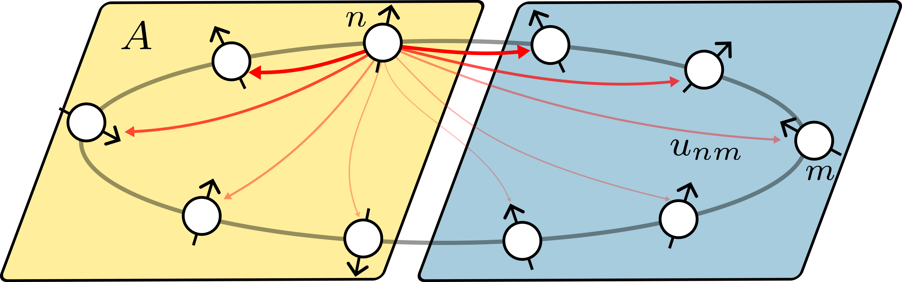
Figure 1: Schematic view of a one-dimensional spin system with long-range interactions and periodic boundary conditions. Here $u_{nm}$ is the interaction potential between site $n$ and $m$. The system is translational invariant, i.e., $u_{nm}$ depends only on the distance $|n-m|$ along the ring. The magnitude of $u_{nm}$ is depicted by the faintness of the arrow. The chain has $L$ sites and periodic boundary conditions. We are interested in the entanglement between a subsystem $A$ containing $L/2$ sites and the rest.

2 Quantum Spherical Model (QSM) with long-range interactions

The spherical model [69] was originally introduced as a simplification of the Ising model, and has established itself as a reference system to investigate collective properties of strongly-interacting systems. Indeed, the spherical model allows for analytical investigation of many-body systems beyond mean-field transitions.

In its quantum formulation, the QSM becomes equivalent to a system of harmonic oscillators subject to a single global constraint. The Hamiltonian of the one-dimensional QSM with periodic boundary conditions is [64, 65, 66, 67]

$$H=\sum_{n=1}^{L}\left[\frac{g}{2}p_{n}^{2}+\frac{1}{2}\sum_{m=1}^{L}u_{nm}x_{n}x_{m}\right].$$ (3)

The operators $x_{n}$ and $p_{n}$ are the conjugated oscillator position and momentum operators, satisfying the canonical commutation relation $[x_{n},p_{m}]=\mathrm{i}\hbar\delta_{nm}$. The oscillators interact through the translation invariant potential $u_{nm}=u(|n-m|)$. To decouple the oscillators, we introduce the Fourier transformed operators $q_{k},\pi_{x}$ as

$$x_{n}=\frac{1}{\sqrt{L}}\sum_{k\in\mathcal{B}}e^{\mathrm{i}kn}q_{k},\qquad p_{n}=\frac{1}{\sqrt{L}}\sum_{k\in\mathcal{B}}e^{-\mathrm{i}kn}\pi_{k}\ ,$$ (4)

with the Brillouin zone $\mathcal{B}=\{0,2\pi/L,...,2\pi(L-1)/L\}$. The Hamiltonian in Eq. (3) then reads

$$H=\sum_{k\in\mathcal{B}}\left[\frac{g}{2}\pi_{k}\pi_{-k}+\frac{1}{2}u(k)q_{k}q_{-k}\right],$$ (5)

with $u(k)$ the Fourier transformed interaction potential. For nearest-neighbor interactions, $u(k)$ is a discretized Laplacian, i.e., $u(k)=2\mu+2(1-\cos k)$. It has been argued that long-range interactions may be introduced by replacing the Laplacian by its fractional counterpart [78, 47] as

$$u(k)=2\mu+\left(2(1-\cos k)\right)^{\frac{\alpha}{2}}.$$ (6)

Indeed, in real space, Eq. (6) corresponds to the interaction potential

$$u(|n-m|)\stackrel{{\scriptstyle|n-m|\to\infty}}{{\simeq}}-\frac{\Gamma\left(1+\alpha\right)}{\pi}\sin\left(\frac{\alpha}{2}\pi\right)\left(\frac{1}{|n-m|}\right)^{\alpha+1},$$ (7)

which is clearly long-range. The strength of the interaction is parametrized by the long-range exponent $\alpha$. Here we consider $0<\alpha<2$, such that the interaction potential satisfies the condition $1+\alpha>d=1$. In this regime, which is sometimes referred to as weak long-range regime, the thermodynamic limit is well-defined as the interactions decay sufficiently fast with distance [44]. The parameter $\mu$ is a Lagrange parameter chosen self-consistently to ensure the spherical constraint as [69, 66, 79, 67]

$$\sum_{n=1}^{L}\left<x_{n}^{2}\right>=L.$$ (8)

This constraint distinguishes the QSM from a simple collection of harmonic oscillators, and is responsible for supporting a quantum phase transition at zero temperature. To pinpoint this transition, we diagonalize the Hamiltonian in Eq. (5) by introducing bosonic ladder operators $b_{k},b^{\dagger}_{k}$ as

$$q_{k}=\alpha_{k}\frac{b_{k}+b_{-k}^{\dagger}}{\sqrt{2}},\qquad\pi_{k}=\frac{\mathrm{i}}{\alpha_{k}}\frac{b_{k}^{\dagger}-b_{-k}}{\sqrt{2}},$$ (9)

with $\alpha_{k}^{4}=g/u(k)$ [67]. Hence, the Hamiltonian $H$ becomes diagonal and Eq. (5) can be written as

$$H=\sum_{k\in\mathcal{B}}E_{k}\left(b_{k}^{\dagger}b_{k}+\frac{1}{2}\right),\qquad E_{k}:=\sqrt{gu(k)}.$$ (10)

To determine the critical behavior of the QSM at zero temperature and to study entanglement properties (see section 3), it is necessary to obtain the position and momentum correlation functions $\mathbb{X}_{nm}$ and $\mathbb{P}_{nm}$ respectively. A straightforward calculation gives [67]

$$\mathbb{X}_{nm} :=\langle x_{n}x_{m}\rangle=\frac{g}{2L}\sum_{k}e^{\mathrm{i}(n-m)k}\frac{1}{E_{k}},$$ (11a)

$$\mathbb{P}_{nm} :=\langle p_{n}p_{m}\rangle=\frac{1}{g}\frac{1}{2L}\sum_{k}e^{-\mathrm{i}(n-m)k}E_{k},$$ (11b)

where $\langle\cdot\rangle$ denotes the ground-state expectation value. In the thermodynamic limit $L\to\infty$ the diagonal components of the correlator $\mathbb{X}_{nm}$ allow to rewrite the spherical constraint (cf. Eq. (8)) as

$$\frac{2}{g}=\frac{1}{L}\sum_{k}\frac{1}{E_{k}}\stackrel{{\scriptstyle L\to\infty}}{{\to}}\int_{0}^{2\pi}\frac{\mathrm{d}k}{2\pi}\frac{1}{E_{k}}.$$ (12)

In the thermodynamic limit Eq. (12) has a finite solution $\mu>0$ as long as the tuning parameter $g$ satisfies $g>g_{c}$. Conversely, for $g\leq g_{c}$ one finds that $\mu$ is identically zero. The nonanalytic behavior of $\mu$ as a function of $g$ determines the critical properties of the model. The quantum critical point at $g_{c}$ marks the transition between a paramagnetic phase at $g>g_{c}$ and a ferromagnetically ordered one at $g<g_{c}$. The critical coupling $g_{c}$ is obtained by imposing the condition $\mu=0$ [66, 67]. Direct integration of the constraint then yields (see A)

$$g_{c}=2^{\alpha+2}\pi\left(\frac{\Gamma\left(1-\alpha/4\right)}{\Gamma\left(1/2-\alpha/4\right)}\right)^{2}.$$ (13)

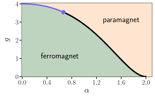
Figure 2: Zero-temperature phase diagram of the quantum spherical model (QSM) with long-range interactions. The plot shows the critical coupling $g_{c}$ as a function of the decay exponent $\alpha$ of the long-range interactions (continuous line). Here we restrict ourselves to $0\leq\alpha<2$, i.e., to the regime of weak long-range interactions, for which the thermodynamic limit is well defined. At $g=g_{c}$ the QSM exhibits a second-order quantum phase transition, which divides a paramagnetic phase from a ferromagnetically ordered one. For $\alpha\geq 2$ interactions are effectively short-ranged, and the QSM is not critical. For $\alpha\leq 2/3$ (dot in the figure) the transition is of mean-field type.

The resulting zero-temperature phase diagram is shown in Fig. 2 for $0\leq\alpha\leq 2$. Notice that for $\alpha>2$ the model becomes effectively short range, and the critical behavior disappears, as expected for a one-dimensional model. One can also show that for $0\leq\alpha\leq 2/3$ the phase transition is of mean-field type, see Ref. [66] or B for further details. Thus, at least for $2/3<\alpha<2$, the QSM supports non-mean-field criticality despite being a Gaussian system. This is due to the nontrivial spherical constraint, see Eq. (8).

Let us now discuss the finite-size scaling of the spherical parameter $\mu$. For finite $L$ Eq. (8) gives a nonzero value of $\mu$ for any $g$. Upon increasing $L$, the spherical parameter $\mu$ retains a finite value for $g>g_{c}$, whereas it vanishes for $g\leq g_{c}$. The precise behaviors of $\mu$ at the critical point $g_{c}$ and in the ordered phase are different. Specifically, in B we show that the finite-size scaling of $\mu$ is given by

$$\mu=\begin{dcases}\quad\frac{\gamma_{\alpha}}{L^{\alpha}},&g=g_{c}\\ \quad\frac{1}{8}\left(\frac{1}{\sqrt{g}}-\frac{1}{\sqrt{g_{c}}}\right)^{-2}\frac{1}{L^{2}},&g<g_{c}.\end{dcases}$$ (14)

Figure 3: Prefactor $\gamma_{\alpha}$ of the finite-size scaling behavior of the spherical parameter $\mu=\gamma_{\alpha}/L^{\alpha}$ at the critical point. Here we plot $\gamma_{\alpha}$ versus the exponent $\alpha$ of the long-range interactions. We only consider the region $2/3<\alpha<2$. Notice the vanishing behavior for $\alpha\to 2$ and $\alpha\to 2/3$. For $\alpha\to 2$ the model becomes short range and there is no critical behavior. For $\alpha\leq 2/3$ the transition becomes of the mean-field type. The curve is obtained by numerically solving Eq. (15).

In Eq. (14) we show only the leading behavior of $\mu$ in the limit $L\to\infty$. Notice that deep in the ferromagnetic phase, i.e., for $g\ll g_{c}$, Eq. (14) yields $\mu\simeq g/(8L^{2})$. The scaling for $g<g_{c}$ is determined solely by the zero mode at $k=0$ in the dispersion $E_{k}$ (cf. Eq. (10)). Notice that from $\mu$ one can define the correlation length $\xi_{\mathrm{corr}}$ of the QSM [66] as $\xi_{\mathrm{corr}}=\mu^{-1/\alpha}$. The constant $\gamma_{\alpha}$ in Eq. (14) is universal, and is obtained by solving the equation (see B)

$$\pi^{-\frac{3}{2}}\Gamma\left(\frac{1}{2}-\frac{1}{\alpha}\right)\Gamma\left(1+\frac{1}{\alpha}\right)(2\gamma_{\alpha})^{\frac{1}{\alpha}-\frac{1}{2}}+(2\gamma_{\alpha})^{-\frac{1}{2}}+4\gamma_{\alpha}^{\frac{1}{\alpha}-\frac{1}{2}}r^{\prime}+4\sum_{k=0}^{\infty}\gamma_{\alpha}^{k}r_{k}=0,$$ (15)

with $r_{k}$ given by

$$r_{k}:=\frac{(-1)^{k}}{k!}\frac{2^{k-1}}{\pi^{\frac{3}{2}}}\Gamma\left(k+\frac{1}{2}\right)\sin\left(\frac{\pi}{4}\alpha(2k+1)\right)\Gamma\left(1-k\alpha-\frac{\alpha}{2}\right)\zeta\left(1-\frac{\alpha}{2}(2k+1)\right),$$ (16)

and $r^{\prime}$ defined as

$$r^{\prime}=-2^{\frac{1}{\alpha}-\frac{5}{2}}\pi^{-\frac{3}{2}}\Gamma\left(\frac{1}{2}-\frac{1}{\alpha}\right)\Gamma\left(1+\frac{1}{\alpha}\right).$$ (17)

In Eqs. (16) and (17) $\Gamma(x)$ is the Euler gamma function, and $\zeta(x)$ is the Riemann zeta function. Importantly, Eq. (15) holds only in the region $2/3<\alpha<2$, in which the critical behavior is not of mean-field type. For $\alpha\to 2/3$ and $\alpha\to 2$, $\gamma_{\alpha}$ vanishes, and it exhibits a maximum at $\alpha\approx 1$. One should also notice that Eq. (15) depends on an infinite number of constants $r_{p}$. Still, it is straightforward to check that $r_{p}$ decays exponentially with increasing $p$, which implies that one can effectively truncate the sum in (15). We show $\gamma_{\alpha}$ as a function of $\alpha$ in Fig. 3. The continuous line is obtained by numerically solving (15). Again, our results hold for $\alpha>2/3$, although they could be straightforwardly generalized to the mean field region $\alpha\leq 2/3$. Moreover, we numerically observed that in the mean-field region (see Fig. 2) $\mu$ still decays as a power law in the large $L$ limit, although we did not extract the precise finite-size scaling behavior.

Importantly, both at criticality and in the ferromagnetic phase the scaling of $\mu$ at leading order for large $L$ depends only on the low-energy properties of the model. Finally, it is interesting to observe that for $\alpha=1$, the critical exponents of the QSM become the same as those of the two-dimensional short-range QSM. Still, the constant $\gamma_{1}$ is not expected to be the same in the two models, because $\gamma_{\alpha}$ depends on the dimensionality and boundary conditions.

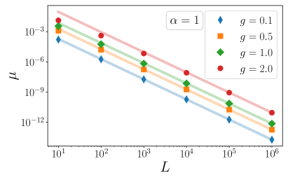
Figure 4: Finite-size scaling of the spherical parameter $\mu$ in the QSM with long-range interactions. We show $\mu$ plotted versus $L$ for $\alpha=1$ and $\alpha=1.5$ (in the left and right panel, respectively). The different symbols correspond to different value of the coupling $g$. All the results are for the ferromagnetic phase at $g<g_{c}$. The continuous lines are the analytical results for $L\to\infty$ (cf. (14)).

In Fig. 4 we numerically verify the finite-size scaling of the spherical parameter (cf. Eq. (14)) in the ferromagnetic phase. Specifically, in the figure we show numerical results for $\mu$ as a function of $L$, obtained by solving Eq. (8). The left and right panels show results for $\alpha=1$ and $\alpha=3/2$, respectively. In both cases $\mu$ decays as a power-law in the limit $L\to\infty$ (notice the logarithmic scale on both axes). In each panel, the different symbols correspond to different values of the coupling $g$. The continuous lines are the analytic results in Eq. (14), and are in agreement with the numerical data in the limit $L\to\infty$. The agreement is perfect deep in the ferromagnetic phase. Finite-size corrections increase upon approaching the critical point, which signals the different scaling as $L^{-\alpha}$ at criticality. As it is clear from Fig. 4, upon approaching criticality, larger system sizes are needed to observe the asymptotic scaling predicted in Eq. (14).

Let us now discuss the finite-size scaling of $\mu$ at the phase transition (continuous line in Fig. 2). Again, we focus on the region $2/3<\alpha<2$, i.e., where the transition is not of mean-field type. Fig. 5 shows numerical results for $\mu$ plotted as a function of $L$. Different symbols correspond to different values of the long-range exponent $\alpha$. The continuous lines are the analytical predictions from Eq. (14), with $\gamma_{\alpha}$ obtained by solving (15) (see Fig. 3). The agreement between the numerical data and the analytical results is perfect. We anticipate that the finite-size scaling of $\mu$ presented here will be useful in section 4 to determine the finite-size scaling of the entanglement gap.

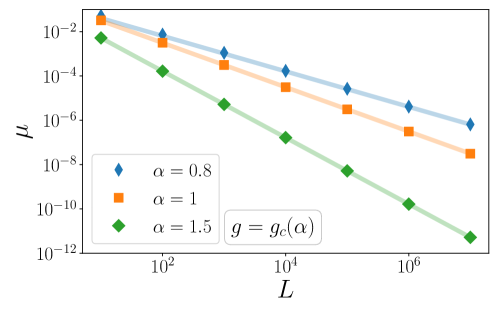
Figure 5: Finite-size scaling of the spherical parameter $\mu$ in the critical long-range QSM: $\mu$ is plotted versus the system size $L$. Different symbols are for different values of the exponent $\alpha$ of the long-range interactions. Here we only consider the case $2/3<\alpha<2$, in which the critical behavior is not of mean-field type. The continuous lines denote the analytic result $\gamma_{\alpha}/L^{\alpha}$, with $\gamma_{\alpha}$ obtained by solving Eq. (15).

3 Entanglement properties of the QSM

Here we summarize the calculation of entanglement-related quantities in the QSM. As discussed in section 2, the QSM is mappable to a system of free bosons with the global spherical constraint, see Eq. (8). This ensures that entanglement related properties can be computed from the bosonic correlation functions [80]. Specifically, the reduced density matrix $\rho_{A}$ of a generic subregion $A$ (see Fig. 1) for a system of free bosons can be written as [80]

$$\rho_{A}=Z^{-1}e^{-{\cal{H}}_{A}},\qquad{\cal{H}}_{A}=\sum_{k}\epsilon_{k}b_{k}^{\dagger}b_{k}.$$ (18)

with ${\cal{H}}_{A}$ the entanglement Hamiltonian, $\epsilon_{k}$ the single-particle entanglement spectrum (ES), and $b_{k}$, $b_{k}^{\dagger}$ the bosonic ladder operators introduced in Eq. (9). The constant $Z$ ensures the normalization of $\rho_{A}$ such that $\mathrm{Tr}(\rho_{A})=1$. The single-particle ES levels $\epsilon_{k}$ are readily related to the eigenvalues of the correlation matrix because the QSM is Gaussian. Again, entanglement properties of Gaussian systems are encoded in the two-point correlation matrices. For free bosons one has to compute the matrices (11a) and (11b), where the chemical potential $\mu$ is self-consistently determined from Eq. (8). To proceed, one has to compute the restricted correlation matrix $\mathbb{C}_{A}$, which is defined as

$$\mathbb{C}_{A}:=\mathbb{X}_{A}\cdot\mathbb{P}_{A},\quad\mathbb{X}_{A}(\mathbb{P}_{A})=\mathbb{X}_{ij}(\mathbb{P}_{ij})\,\,\mathrm{with}\,\,i,j\in A.$$ (19)

The entanglement spectrum and the eigenvalues $\epsilon_{k}$ are related to the eigenvalues $e_{k}$ of $\mathbb{C}_{A}$ as [80]

$$\sqrt{e_{k}}=\frac{1}{2}\coth\left(\frac{\epsilon_{k}}{2}\right).$$ (20)

The ES of the QSM is then obtained by populating the single-particle levels $\epsilon_{k}$ (cf. (20)). We find

$$\xi\left(\{\beta_{k}\}\right)=\ln(Z)+\sum_{j}\beta_{j}\epsilon_{j}.$$ (21)

Here $\beta_{k}\in\mathbb{N}$ is the number of bosons in the single-particle ES level $\epsilon_{k}$, and $Z$ is the same normalization factor as in (18), viz.,

$$Z=\prod_{j=1}^{|A|}\left(\sqrt{e_{j}}+1/2\right),$$ (22)

where $|A|$ is the size of $A$. The lowest ES level corresponds to $\beta_{j}=0$ for any $j$. Let us assume that the single-particle ES levels are ordered as $\epsilon_{1}<\epsilon_{2}<\cdots<\epsilon_{|A|}$. The first excited ES level is obtained by populating the smallest single particle level $\epsilon_{1}$. Thus, the lowest entanglement gap $\delta\xi$ (Schmidt gap) is defined as

$$\delta\xi=\xi_{1}-\xi_{0}=\epsilon_{1},$$ (23)

and $\epsilon_{1}$ is related to the eigenvalue $e_{1}$ of $\mathbb{C}_{A}$ via Eq. (20).

4 Finite-size scaling of the entanglement gap in the ordered phase of the long-range QSM

Our main result is that in the ordered phase of the long-range QSM (see Fig. 2) the eigenvalue $e_{1}$ of the restricted correlation matrix $\mathbb{C}_{A}$ (cf. Eq. (19)) in the large $L$ limit scales as

$$e_{1}=\chi_{A}^{x}\chi_{A}^{t},$$ (24)

where $\chi_{A}^{x,t}$ are the coordinate and momentum “susceptibilities” defined as

$$\chi_{A}^{x}:=\langle 1|\mathbb{X}|1\rangle_{A},\quad\chi_{A}^{t}:=\langle 1|\mathbb{P}|1\rangle_{A}.$$ (25)

Here $\mathbb{X}$ and $\mathbb{P}$ are defined in Eqs. (11a) and (11b), respectively. Moreover, we introduced the normalized flat vector $|1\rangle:=(1,1,\cdots,1)/\sqrt{L_{A}}$ restricted to subsystem $A$. The expectation values in Eq. (25) are defined as

$$\langle 1|\mathbb{X}(\mathbb{P})|1\rangle_{A}:=\frac{1}{L_{A}}\sum_{n,m=1}^{L_{A}}\mathbb{X}_{nm}(\mathbb{P}_{nm}).$$ (26)

To proceed, it is crucial to observe that for $g<g_{c}$ the system develops ferromagnetic order, for any value of $\alpha<2$. This is reflected in the presence of a zero mode in the dispersion of the model at $k=0$ and $k=2\pi$ (cf. Eq. (10)). In C we derive analytically that this zero mode yields that $\chi_{A}^{x}\simeq L$ for large $L$ (see Eq. (94)). The same volume scaling $\simeq L$ is observed in short-range quantum spherical models that exhibit magnetic order [77, 68, 36]. This reflects the fact that, although the dispersion of the model is dramatically affected by the long-range interactions, the leading behavior of the magnetic susceptibility is dominated by the zero mode, similar to the short-range case. Now, let us decompose $\mathbb{X}_{A}$ as

$$\mathbb{X}_{A}=\chi_{A}^{x}|1\rangle\langle 1|+\mathbb{X}^{\prime}_{A},$$ (27)

where $\chi_{A}^{x}$ is given in Eq. (25), and $|1\rangle$ is the flat vector restricted to $A$. We exploit the fact that $\chi_{A}^{x}={\mathcal{O}}(L)$ and consider the transposed correlation matrix $\mathbb{C}_{A}^{T}=\mathbb{P}_{A}\cdot\mathbb{X}_{A}$ (cf. Eq. (19)). By using Eq. (27), we obtain

$$\mathbb{P}_{A}\cdot\mathbb{X}_{A}=\chi_{A}^{x}\mathbb{P}_{A}|1\rangle\langle 1|+\mathbb{P}_{A}\cdot\mathbb{X}^{\prime}_{A}.$$ (28)

We can now neglect the second term in Eq. (28) because it is subleading compared to the first one. Importantly, the matrix $\mathbb{P}_{A}\cdot\mathbb{X}_{A}$ is not hermitian. However, in the limit $L\to\infty$ it is easy to identify left and right eigenvectors, $\ket{u_{R}}$ and $\bra{u_{L}}$ respectively, by inspection. They are given by

$$|u_{R}\rangle=\mathbb{P}_{A}|1\rangle,\quad\langle u_{L}|=\langle 1|,$$ (29)

as can be seen by directly applying $\mathbb{C}_{A}^{T}$ to them, viz.,

$$\mathbb{C}_{A}^{T}\ket{u_{R}}\simeq\langle 1|\mathbb{P}_{A}|1\rangle\chi_{A}^{x}\mathbb{P}_{A}|1\rangle,\quad\bra{u_{L}}\mathbb{C}_{A}^{T}\simeq\chi_{A}^{x}\bra{1}\mathbb{P}_{A}\ket{1}\bra{1}.$$ (30)

As it is now clear from Eq. (28), the largest eigenvalue of $e_{1}$ of $\mathbb{C}_{A}$ is

$$e_{1}=\chi_{A}^{x}\langle 1|\mathbb{P}_{A}|1\rangle=\bra{1}\mathbb{X}_{A}\ket{1}\bra{1}\mathbb{P}_{A}\ket{1}.$$ (31)

We should mention that the same decomposition in Eq. (27) was employed in Ref. [81] to analyze the contribution of the zero mode to the ES in the harmonic chain. Moreover, the same decomposition has been employed to study the entanglement gap in the ordered phase of the two-dimensional quantum spherical model [68, 36] (see also [77]).

Eq. (31) shows that the finite-size scaling of the entanglement gap in the ferromagnetic phase is governed by the zero mode of the dispersion in Eq. (10). Specifically, as it is clear from the lack of spatial structure of $|1\rangle$, $\chi_{A}^{x}$ is directly determined by the zero mode. On the other hand, the susceptibility $\chi_{A}^{t}$ is sensitive to the dispersion of the model. Crucially, both $\chi_{A}^{x}$ and $\chi_{A}^{t}$ can be determined analytically in the large $L$ limit. The derivation employs standard tools such as Poisson’s summation formula and the Mellin transform, and it is reported in B,  C and D. The leading and first subleading contributions of $\chi_{A}^{x}$ in the large $L$ limit are

$$\chi_{A}^{x}\simeq\frac{1}{4}\sqrt{\frac{g}{2\mu}}+\frac{\sqrt{g}}{\pi}\sin\left(\frac{\pi}{4}\alpha\right)\Gamma\left(-1-\frac{\alpha}{2}\right)\left(2^{1-\frac{\alpha}{2}}-2^{3}\right)\zeta\left(-1-\frac{\alpha}{2}\right)L^{\frac{\alpha}{2}},$$ (32)

where $\zeta(x)$ is the Riemann zeta function, and $\Gamma(x)$ is the Euler gamma function. The first term in Eq. (32) is the zero-mode contribution, which is simply obtained by isolating the term with $k=0$ in Eq. (11a). Since $\mu={\mathcal{O}}(L^{-2})$ in the ordered phase (see Fig. 4), this term is ${\mathcal{O}}(L)$. The second term is ${\mathcal{O}}(L^{\alpha/2})$, and it is subleading because $0<\alpha<2$. In Eq. (32) we neglected $o(L^{\alpha/2})$ terms, which are reported in C. Eq. (32) holds at the critical point as well, although it is not useful to determine the scaling of the entanglement gap since Eq. (24) does not hold true at criticality. At the critical point one has $\mu={\mathcal{O}}(L^{-\alpha})$, which implies that both terms in Eq. (32) are of the same order. It is important to stress that both at the critical point, as well as in the ordered phase, the terms in Eq. (32) depend only on the low-energy part of the dispersion of the QSM. In particular, the second term in Eq. (32) does not depend on the cutoff $\Lambda$ introduced to regularize the behavior of the correlators. The second term in Eq. (32) is one of an infinite number of terms that determine the universal behavior upon approaching the critical point. These terms are reported in C.

Similarly, we obtain the leading behavior for $\chi_{A}^{t}$ as (see D)

$$\chi_{A}^{t}\simeq\frac{1}{\sqrt{g}}\frac{2}{\pi}\left(4-2^{\frac{\alpha}{2}}\right)\Gamma\left(\frac{\alpha}{2}-1\right)\sin\left(\frac{\pi}{4}\alpha\right)\zeta\left(\frac{\alpha}{2}-1\right)L^{-\frac{\alpha}{2}}$$ (33)

Clearly, $\chi_{A}^{t}$ vanishes in the limit $L\to\infty$, in contrast to $\chi_{A}^{x}$ (cf. Eq. (32)). Again, the behavior of $\chi_{A}^{t}$ is determined by the universal low-energy part of the dispersion of the model. Using Eqs. (31), (32) and (33), we obtain

$$e_{1}\simeq C^{\prime}_{\alpha}L^{1-\frac{\alpha}{2}}=\frac{1}{\pi}\left(\frac{1}{\sqrt{g}}-\frac{1}{\sqrt{g}}\right)\left(4-2^{\frac{\alpha}{2}}\right)\Gamma\left(\frac{\alpha}{2}-1\right)\sin\left(\frac{\pi}{4}\alpha\right)\zeta\left(\frac{\alpha}{2}-1\right)L^{1-\frac{\alpha}{2}}.$$ (34)

As it is clear from Eq. (34) the eigenvalue $e_{1}$ diverges in the limit $L\to\infty$ because $0<\alpha<2$. Moreover, the constant $C^{\prime}_{\alpha}$ depends on the low-energy properties of the QSM. Finally, we obtain that the entanglement gap $\delta\xi$ in the large $L$ limit vanishes as

$$\delta\xi\simeq C_{\alpha}L^{-\frac{1}{2}+\frac{\alpha}{4}},\quad\mathrm{with}\,\,C_{\alpha}=\frac{1}{\sqrt{C^{\prime}_{\alpha}}},$$ (35)

with $C^{\prime}_{\alpha}$ as defined in Eq. (34).

It is interesting to compare the result in Eq. (34) with the scaling of the entanglement gap in the magnetically ordered phase of the two-dimensional QSM [36]. Similar to Eq. (35), $\delta\xi$ exhibits a power-law decay with $L$. Precisely, for the $2D$ QSM one has the behavior [36]

$$\delta\xi\simeq\frac{\Omega}{\sqrt{L\ln(L)}},$$ (36)

where $\Omega$ is a constant that depends on the geometry of the bipartition and on the low-energy properties of the QSM. In particular $\Omega$ is dramatically affected by the presence of corners in the boundary between $A$ and the rest. Notice that the multiplicative logarithmic correction in Eq. (36), which reflects a multiplicative logarithmic correction in $e_{1}$, is a genuine consequence of the model being two-dimensional, and it is absent in the $1D$ long-range QSM.

Finally, it is interesting to observe that on the critical line (see Fig. 2) one has that $\mu={\mathcal{O}}(L^{-\alpha})$. Thus, by using Eq. (34) one obtains that $e_{1}\simeq{\mathcal{O}}(1)$. However, this is not accurate because we numerically observe that at criticality $e_{1}$ diverges, although slowly, signaling that the entanglement gap vanishes at criticality as well. This is somewhat similar in the $2D$ QSM [68], where the same approximation from Eq. (27) leads to an inaccurate scaling for the entanglement gap. The reason is that at the critical point the eigenvector of $\mathbb{X}$ exhibits a non trivial structure, i.e., it is different from the flat vector $|1\rangle$.

5 Numerical benchmarks

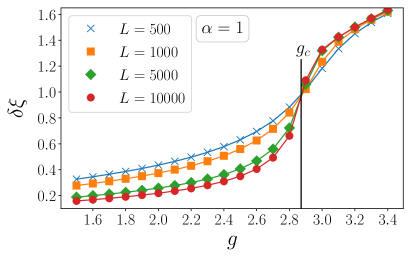
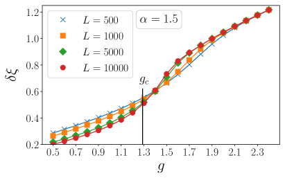
Figure 6: Lowest entanglement gap $\delta\xi$ in the ground-state ES of the QSM with long-range interactions. Here we consider the half-chain ES (see Fig. 1), plotting $\delta\xi$ versus the coupling $g$. The left and right panels correspond to $\alpha=1$ and $\alpha=1.5$, respectively. The different symbols are for different system size $L$. The vertical lines mark the quantum critical point at $g_{c}$. In the paramagnetic phase for $g>g_{c}$, $\delta\xi$ attains a finite value in the limit $L\to\infty$. For $g\leq g_{c}$ the entanglement gap $\delta\xi$ vanishes in the limit $L\to\infty$.

Here we provide numerical benchmarks of the results of section 4. We start discussing the general structure of the entanglement gap across the phase diagram of the QSM (see Fig. 2). In Fig. 6 we show the entanglement gap $\delta\xi$ as a function of the quantum coupling $g$ across the phase transition. The data are obtained by computing the correlation functions in Eq. (19) with the spherical parameter $\mu$ obtained by numerically solving Eq. (8), and by using Eq. (23). The left and right panel show results for $\alpha=1$ and $\alpha=3/2$, respectively. The different symbols correspond to different system sizes $500\leq L\leq 10000$. In Fig. 6 we consider the bipartition with $L_{A}=L/2$ (see Fig. 1). The vertical lines in Fig. 6 mark the critical coupling $g_{c}$. For $g>g_{c}$ the entanglement gap $\delta\xi$ attains a finite value in the limit $L\to\infty$ as can be seen from Fig. 7.

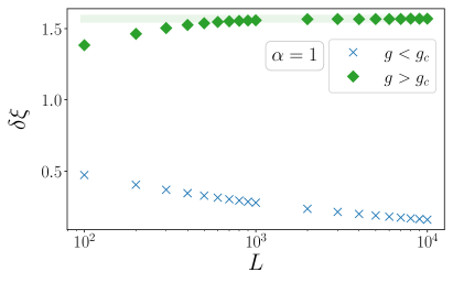
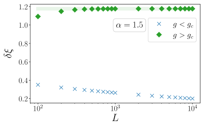
Figure 7: Qualitative behavior of the entanglement gap. Exemplary data from Fig. 6 for the entanglement gap $\delta\xi$ are shown in the ferromagnetic and in the paramagnetic phase. In the ferromagnetic phase the gap vanishes, albeit slowly. Conversely, in the paramagnetic phase the gap remains finite.

On the other hand, in the ordered phase for $g<g_{c}$ the data suggests a vanishing $\delta\xi$ in the limit $L\to\infty$, although sizeable finite $L$ effects are visible.

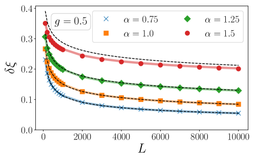
Figure 8: Finite-size scaling of the lowest entanglement gap $\delta\xi$ in the ferromagnetic phase of the long-range QSM. We plot $\delta\xi$ versus $L$ at fixed $g=1/2$. The results are for the half-system ES (see Fig. 1). Different symbols correspond to different values of the long-range exponent $\alpha$. The continuous lines are obtained by using (24). The dash-dotted lines are obtained from the analytic results (34) in the large $L$ limit.

The finite-size scaling of $\delta\xi$ is investigated in Fig. 8 plotting $\delta\xi$ versus $L$ for fixed $g=1/2$, i.e., in the ferromagnetic phase. The different symbols denotes results for different values of the long-range exponent $\alpha$. For all the values of $\alpha$ considered, $\delta\xi$ exhibits vanishing behavior in the limit $L\to\infty$. The continuous line in Fig. 8 is the prediction obtained by numerically computing $\chi_{A}^{x}$ and $\chi_{A}^{t}$ (cf. Eq. (25)), and by employing (34). The agreement between the lattice results and the analytic results in the asymptotic limit $L\to\infty$ is perfect. Finally, the dash-dotted line in Fig. 8 is Eq. (35). The data are in perfect agreement with (35), except for $\alpha=1.5$, for which some deviations are visible. These are attributed to the finite $L$. Indeed, similar deviations are also visible for $\mu$ in Fig. 4, where we show much larger system sizes up to $L\approx 10^{6}$.

6 Conclusions

We characterized the finite-size scaling of the entanglement gap in the long-range $1D$ quantum spherical model. Our main result is given by Eq. (35). We showed that in the ferromagnetically ordered phase of the long-range QSM the entanglement gap vanishes in the thermodynamic limit as $\simeq C_{\alpha}L^{-1/2+\alpha/4}$. The prefactor $C_{\alpha}$ of the decay depends only on the low-energy properties of the model. This behavior is different from the $2D$ quantum spherical model, where the power-law decay of the entanglement gap is accompanied by multiplicative logarithmic corrections [36].

Let us now mention some possible future directions. First, it would be interesting to determine the finite-size scaling of the entanglement gap on the critical line as a function of the long-range exponent $\alpha$. This is in general a challenging task because Eq. (24) is not valid at criticality. An interesting question is whether it is possible to determine the behavior of the distribution of the ES levels [39], and how it is affected by the long-range interactions. The main challenge is that Conformal Field Theory does not hold in the presence of long range interactions. One of our main results is Eq. (31), which confirms that there is a robust relationship between the entanglement gap and standard witnesses of magnetic order, such as $\chi_{A}^{x}$ and $\chi_{A}^{t}$. It would be important to understand whether Eq. (31) survives for the $O(N)$ models away from the $N\to\infty$ limit. It would be also interesting to investigate the effects of disorder on entanglement properties of the long-range QSM, by using the replica trick to perform disorder averages [82, 83, 84, 85, 86]. Another important research direction is to investigate entanglement scaling after quantum quenches in the long-range QSM, using the results of Refs. [87, 88, 89, 90]. Finally, it would be interesting to investigate the negativity spectrum [43, 91, 92] in the long-range QSM.

Appendix A Critical coupling $g_{c}(\alpha)$

Here we derive for generic $\alpha$ the critical coupling $g_{c}$ of the second order phase transition that divides the paramagnetic phase for $g>g_{c}$ from the ordered phase at $g<g_{c}$ (see Fig. 2).

Let us start with the two-point auto-correlation function [77]

$$\mathbb{X}_{nn}=\frac{g}{2L}\sum_{k\in\mathcal{B}}\frac{1}{E_{k}}.$$ (37)

The spherical constraint, Eq. (13), in the thermodynamic limit $L\to\infty$ reads

$$1=\int_{0}^{2\pi}\frac{\mathrm{d}k}{2\pi}\frac{\sqrt{g}/2}{\sqrt{2\mu+\left(2(1-\cos k)\right)^{\frac{\alpha}{2}}}}.$$ (38)

In order to extract $g_{c}(\alpha)$ we directly integrate the spherical constraint for $\mu=0$ and find

$$\frac{2}{g_{c}}=\int_{0}^{2\pi}\frac{dk}{2\pi}\frac{1}{E_{k}}=\frac{2^{-\frac{\alpha}{2}}\Gamma\left(1/2-\alpha/4\right)}{\sqrt{g_{c}\pi}\Gamma\left(1-\alpha/4\right)}.$$ (39)

Thus, we obtain

$$g_{c}=2^{\alpha+2}\pi\left(\frac{\Gamma\left(1-\alpha/4\right)}{\Gamma\left(1/2-\alpha/4\right)}\right)^{2}.$$ (40)

The behavior of $g_{c}$ as a function of $\alpha$ is reported in Fig. 2. Notice that we integrated over the full Brillouin zone to obtain $g_{c}$, which reflects that $g_{c}$ is non universal.

Appendix B Finite-size scaling of the spherical parameter

Let us now extract the finite-size scaling (FSS) of the spherical parameter $\mu$, which is determined by solving

$$\frac{2}{\sqrt{g}}=\frac{1}{L}\sum_{n=0}^{L-1}\frac{1}{\sqrt{2\mu+(2(1-\cos\left(2\pi n/L\right)))^{\alpha/2}}}.$$ (41)

The strategy is to use Poisson’s summation formula

$$\sum_{n=a}^{b}f(n)=\frac{f(a)+f(b)}{2}+\int_{a}^{b}f(x){\mathrm{d}}x+2\sum_{p=1}^{\infty}\int_{a}^{b}f(x)\cos(2\pi px){\mathrm{d}}x$$ (42)

to split (41) into a thermodynamic contribution and a finite-size one. It is useful to observe that in our case (cf. (41)) $a=0$ and $b=L-1$ and that $f(0)=f(L)$. Thus, it is convenient to add and subtract in (42) the term with $n=b+1$. This allows us to get rid of the boundary contribution in the right-hand-side of (42). This means that we can use the modified version of the Poisson summation formula as

$$\sum_{n=a}^{b}f(n)=\int_{a}^{b+1}f(x){\mathrm{d}}x+2\sum_{p=1}^{\infty}\int_{a}^{b+1}f(x)\cos(2\pi px){\mathrm{d}}x,\quad\mathrm{if}\,\,f(a)=f(b+1).$$ (43)

By using (43) we can rewrite (41) as

$$\frac{2}{\sqrt{g}}=\frac{1}{L}\int_{0}^{L}\frac{\mathrm{d}x}{\sqrt{2\mu+\left(2(1-\cos(2\pi x/L))\right)^{\alpha/2}}}\\ +\frac{2}{L}\sum_{n=1}^{\infty}\int_{0}^{L}\frac{\cos\left(2\pi nx\right)\mathrm{d}x}{\sqrt{2\mu+\left(2(1-\cos(2\pi x/L))\right)^{\alpha/2}}}$$ (44)

For the remainder of this section, we work in the long wavelength approximation in which we expand $\cos(k)\approx 1-k^{2}/2$ in the denominators in (44). This approximation affects the behavior of nonuniversal quantities at the transition, such as the value of the critical coupling. In the ferromagnetic phase the long-wavelength approximation affects quantities that depend on the full dispersion of the model. However, as we are going to verify, the behavior of the entanglement gap is sensitive only to the lower-energy properties of the dispersion. This means that the results that we are going to derive apply to the model with the cosine dispersion as well.

In the long-wavelength approximation, we can rewrite (44) as

$$\frac{1}{\sqrt{g}}=\int_{0}^{\Lambda}\frac{\mathrm{d}k}{2\pi}\frac{1}{\sqrt{2\mu+k^{\alpha}}}+2\sum_{n=1}^{\infty}\int_{0}^{\Lambda}\frac{\mathrm{d}k}{2\pi}\frac{\cos\left(nkL\right)}{\sqrt{2\mu+k^{\alpha}}}.$$ (45)

Here after applying the long wavelength approximation we multiplied the right-hand-size by two to account for the fact that the two singularities at $k=0$ and $k=2\pi$ in the original dispersion contribute equally. Here we also extend the Brillouin zone from $[0,2\pi]\to[0,\Lambda)$, introducing the ultraviolet cutoff $\Lambda$. To proceed, we need to extract the large $L$ behavior of the two terms in (45). The integral in the first term in (45) is readily evaluated as in section A. We find

$$\int_{0}^{\Lambda}\frac{\mathrm{d}k}{2\pi}\frac{1}{\sqrt{2\mu+k^{\alpha}}}\stackrel{{\scriptstyle\mu\to 0}}{{\simeq}}\frac{2}{\sqrt{g_{c}}}+\frac{\Gamma\left(\frac{1}{2}-\frac{1}{\alpha}\right)\Gamma\left(1+\frac{1}{\alpha}\right)}{2\pi^{3/2}}\left(2\mu\right)^{\frac{1}{\alpha}-\frac{1}{2}}.$$ (46)

Here we considered the limit $\mu\to 0$ because we are interested in the magnetically ordered phase and in the critical point, where $\mu=0$ in the thermodynamic limit $L\to\infty$. In (46) we identified the critical coupling $g_{c}$ as $g_{c}=4\pi^{2}(2-\alpha)^{2}/\Lambda^{2-\alpha}$. Notice that $g_{c}$ depends on the cutoff $\Lambda$, as expected because it is a nonuniversal quantity. On the other hand, the second term in (46) does not depend on $\Lambda$. We also checked that higher orders in the expansion in the limit $\mu\to 0$ would depend on the cutoff $\Lambda$. The leading order in $\mu$ reveals the onset of mean-field for $\alpha\leq 2/3$.

The analysis of the second term on the right-hand side in (45) is more involved and can be performed by employing the Mellin transform [94]. To proceed, we first define the function $f(n)$ as

$$f(n):=\int_{0}^{\Lambda}\frac{\mathrm{d}k}{2\pi}\frac{\cos(kLn)}{\sqrt{2\mu+k^{\alpha}}},$$ (47)

and analyze the series $\sum_{n=1}^{\infty}f(n)$ (cf. (45)) by using standard regularization techniques [95]. The Mellin transform $\hat{g}(s)$ of a function $g(x)$ is defined as

$$\hat{g}(s)=\int_{0}^{\infty}\mathrm{d}x\,g(x)x^{s-1}.$$ (48)

The inverse of the Mellin transform is performed as

$$g(x)=\frac{1}{2\pi\mathrm{i}}\int_{c-\mathrm{i}\infty}^{c+\mathrm{i}\infty}\mathrm{d}s\,x^{-s}\hat{g}(s),$$ (49)

where $c$ is chosen in the so-called fundamental strip.

For the function $f(n)$ (cf. (47)) we obtain in the limit $\mu\to 0$

$$\hat{f}(s)\simeq\frac{(2\mu)^{\frac{2-\alpha-2s}{2\alpha}}}{2\pi^{3/2}\alpha L^{s}}\Gamma\left(\frac{1}{2}+\frac{s-1}{\alpha}\right)\Gamma\left(\frac{1-s}{\alpha}\right)\cos\left(\frac{\pi}{2}s\right)\Gamma(s).$$ (50)

Again, in the expansion around $\mu=0$ in (50), we neglect all the higher-order terms that depend on the cutoff $\Lambda$. The condition that the integral over $k$ in (47) is defined for $k\to 0$ implies that $\mathrm{Re}(s)<1$. On the other hand, the condition that the integral is well-defined at $\Lambda\to\infty$ implies that $\mathrm{Re}(s)>1-\alpha/2$. As we have a finite cutoff $\Lambda$ and we are not interested in cutoff-dependent contributions, we have the condition $\mathrm{Re}(s)<1$. Importantly, as it is clear from (50) we can extend the fundamental strip beyond $s=1$ because the cosine function removes the simple pole of $\Gamma((1-s)/\alpha)$ at $s=1$. We can now write the series $\sum_{n=1}^{\infty}f(n)$ (cf. (45)) as

$$\sum_{n=1}^{\infty}f(n)=\frac{1}{2\pi\mathrm{i}}\int_{c-\mathrm{i}\infty}^{c+\mathrm{i}\infty}\mathrm{d}s\,\hat{f}(s)\sum_{n=1}^{\infty}n^{-s}=\frac{1}{2\pi\mathrm{i}}\int_{c-\mathrm{i}\infty}^{c+\mathrm{i}\infty}\mathrm{d}s\,\hat{f}(s)\zeta(s).$$ (51)

Here we used the definition of the Riemann zeta function $\zeta(s)$, and we have $\mathrm{Re}(c)>1$.

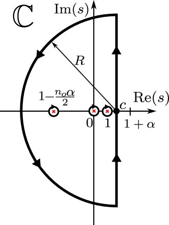
Figure 9: Integration contour in the complex plane $\mathrm{Im}(s)$ versus $\mathrm{Re}(s)$ used to compute the inverse Mellin transform in (51). The vertical part of the contour corresponds to fixed $\mathrm{Re}(s)=c$, with $1<c<1+\alpha$, where the integrand in (51) is analytic. The crosses are the poles of the integrand. The simple pole at $s=1$ is due to the Riemann zeta function in (51). The poles at $s=0$ and at $s=1-n_{o}\alpha/2$ are due to the functions $\Gamma(s)$ and $\Gamma(1/2-(s-1)/\alpha)$ in (50). Here $n_{o}:=2p+1$ with $p\in\mathbb{N}$. The remaining poles of (51) are removed by $\zeta(s)$ and by $\cos(\pi s/2)$.

Notice that the fact that the integrand in (51) is analytic for $1<\mathrm{Re}(s)<1+\alpha$ ensures that it is possible to define the fundamental strip for $s>1$. To proceed, we perform the integral over $s$ in (51) in the complex plane. To choose the suitable contour we observe that the spherical parameter decays algebraically with increasing $L$, both at the critical point and in the ordered phase. This suggests the finite-size scaling behavior of $\mu$ as $\mu\propto L^{-\sigma}$ with $\sigma>0$. By using (50), this suggests the scaling of $\hat{f}(s)$ as

$$\hat{f}(s)\propto L^{s(\sigma/\alpha-1)}L^{\sigma(\alpha-2)/(2\alpha)}.$$ (52)

Since $\alpha<2$, the second term in (52) always decays for $L\to\infty$, whereas the behavior of the first one is different for $\sigma\geq\alpha$ and for $\sigma<\alpha$. However, we can exclude that $\sigma<\alpha$ because for $\alpha\to 0$, i.e., for the infinite-range model, this would yield a finite $\mu$. Hence, we consider $\sigma\geq\alpha$. Thus, a consistent finite-size analysis suggests to close the complex contour at $\operatorname{Re}(s)\to-\infty$, as shown in Fig. 9. The integral is determined by the singularities within the contour, which we now discuss.

First, the Riemann zeta function $\zeta(s)$ has a simple pole at $s=1$. The gamma function $\Gamma(s)$ has poles at $s=-n$ with $n\in\mathbb{N}$ an integer. The function $\Gamma((1-s)/\alpha)$ has poles at $s=n\alpha+1$, with $n\in\mathbb{N}/\{0\}$, and at $s=1-(2n+1)\alpha/2$, with $n\in\mathbb{N}$. Notice that the poles at $1+n\alpha$ are not within the integration contour (see Fig. 9), and we can neglect them. Moreover, the poles at $s=-n_{o}$ with $n_{o}$ odd positive integers cancel out with the term $\cos(\pi/2s)$ in (51). On the other hand, the poles at $s=-n_{e}$ with $n_{e}$ an arbitrary positive even integer do not contribute because $\zeta(-n_{e})=0$. In conclusion, the only poles $s^{*}$ that contribute to the integral in (51) are

$$s^{*}=\left\{\begin{array}[]{cc}0&\\ 1&\\ 1-\frac{(2p+1)\alpha}{2}&p\in\mathbb{N}\end{array}\right.$$ (53)

Thus, since the contribution of the circle in the contour in Fig. 9 vanishes for $R\to\infty$, from (51) we obtain that

$$\sum_{n=1}^{\infty}f(n)=\sum_{\mathrm{poles}\,s^{*}}\mathrm{Res}(\hat{f}(s)\zeta(s),s^{*}),$$ (54)

where $s^{*}$ are given in (53). Specifically, the pole at $s=1$ gives the contribution

$$\operatorname{Res}(\hat{f}(s)\zeta(s),s=1)=\frac{(2\mu)^{-\frac{1}{2}}}{4L},$$ (55)

where we used that the residue of $\zeta(s)$ at $s=1$ is one. To proceed, we observe that the singularities of $\Gamma(s)$ at $s=-p$ with $p$ an integer are simple poles, with residue

$$\mathrm{Res}(\Gamma(s),-p)=\frac{(-1)^{p}}{p!}.$$ (56)

This allows us to obtain the contribution at $s^{*}=0$ (cf. (53)) as

$$\mathrm{Res}(\hat{f}(s)\zeta(s),0)=\mu^{-\frac{1}{2}+\frac{1}{\alpha}}r^{\prime},\quad\mathrm{with}\,\,r^{\prime}:=-\frac{2^{-\frac{5}{2}+\frac{1}{\alpha}}}{\pi^{\frac{3}{2}}}\Gamma\left(\frac{1}{2}-\frac{1}{\alpha}\right)\Gamma\left(1+\frac{1}{\alpha}\right).$$ (57)

Finally, let us consider the poles at $s=1-(2p+1)\alpha/2$. We obtain that

$$\mathrm{Res}\left(\hat{f}(s)\zeta(s),1-\frac{2p+1}{2}\alpha\right)=\mu^{p}L^{\alpha\left(p+\frac{1}{2}\right)-1}r_{p},$$ (58)

with $r_{p}$ defined as

$$r_{p}:=\frac{(-1)^{p}2^{p-1}}{\pi^{\frac{3}{2}}p!}\Gamma\left(p+\frac{1}{2}\right)\sin\left(\frac{1}{4}\pi\alpha(2p+1)\right)\Gamma\left(-p\alpha-\frac{\alpha}{2}+1\right)\zeta\left(1-\frac{1}{2}(2p+1)\alpha\right).$$ (59)

Finally, putting together (55) (57) and (59) we obtain

$$\sum_{n=1}^{\infty}f(n)=\frac{(2\mu)^{-\frac{1}{2}}}{4L}+\mu^{-\frac{1}{2}+\frac{1}{\alpha}}r^{\prime}+\sum_{p=0}^{\infty}\mu^{p}L^{\alpha\left(p+\frac{1}{2}\right)-1}r_{p}.$$ (60)

Now, it is important to notice that at the critical point we expect $\mu\propto L^{-\alpha}$. This implies that all the three contributions in (60) are of the same order $L^{\alpha/2-1}$. Oppositely, in the ferromagnetically ordered phase one has $\mu\propto L^{-2}$, implying that in the large $L$ limit the first term in (60) is the leading one, whereas the other ones are suppressed. Thus, to obtain the leading behavior of $\mu$ for $g<g_{c}$ it is sufficient to replace (41) with the equation

$$\frac{1}{\sqrt{g}}-\frac{1}{\sqrt{g_{c}}}\simeq\frac{(2\mu)^{-\frac{1}{2}}}{2L},$$ (61)

which allows us to readily find

$$\mu=\frac{1}{8}\left(\frac{1}{\sqrt{g}}-\frac{1}{\sqrt{g_{c}}}\right)^{-2}\frac{1}{L^{2}}+o(L^{-2}),\quad\mathrm{for}\,\,g<g_{c}.$$ (62)

In particular, deep in the ferromagnetic phase, we find

$$\mu\simeq\frac{g}{8}\frac{1}{L^{2}}.$$ (63)

To extract the finite-size scaling of $\mu$ at the critical point, let us define $\gamma_{\alpha}$ as

$$\mu=\frac{\gamma_{\alpha}}{L^{\alpha}}.$$ (64)

After substituting the ansatz (64) in the gap equation (45) and setting $g=g_{c}$, we obtain the equation for $\gamma_{\alpha}$ as

$$\frac{\Gamma\left(\frac{1}{2}-\frac{1}{\alpha}\right)\Gamma\left(1+\frac{1}{\alpha}\right)}{\pi^{3/2}}(2\gamma_{\alpha})^{\frac{1}{\alpha}-\frac{1}{2}}+(2\gamma_{\alpha})^{-\frac{1}{2}}+4\gamma_{\alpha}^{-\frac{1}{2}+\frac{1}{\alpha}}r^{\prime}+4\sum_{k=0}^{\infty}\gamma_{\alpha}^{k}r_{k}=0$$ (65)

We observe that since $r_{k}$ are suppressed exponentially upon increasing $k$, we can truncate (65) by keeping the first $k_{\mathrm{max}}$ terms in the sum. A numerical solution of (65) as a function of $\alpha$ is shown in Fig. 3.

Appendix C Finite-size scaling of the susceptibility $\chi_{A}^{x}$

Here we derive the flat vector expectation values of the position correlation matrix $\mathbb{X}_{nm}$ (cf. (11a)) given as

$$\mathbb{X}_{nm}=\frac{\sqrt{g}}{2L}\sum_{k=0}^{L-1}\frac{e^{\mathrm{i}(n-m)2\pi k/L}}{\sqrt{2\mu+{\omega}_{k}}},\quad\text{with}\quad\omega_{k}=[2(1-\cos(2\pi k/L))]^{\frac{\alpha}{2}}.$$ (66)

We use Poisson’s summation formula (43) to decompose the position correlator into a thermodynamic and a finite-size component, viz.,

$$\mathbb{X}_{nm}=\mathbb{X}^{\rm(th)}_{nm}+\mathbb{X}^{\rm(L)}_{nm}.$$ (67)

Specifically, we have

$$\mathbb{X}^{\rm(th)}_{nm}=\frac{\sqrt{g}}{2}\int_{0}^{2\pi}\frac{\mathrm{d}k}{2\pi}\frac{e^{\mathrm{i}(n-m)k}}{\sqrt{2\mu+\omega_{k}}}$$ (68)

$$\mathbb{X}^{\rm(L)}_{nm}=\sqrt{g}\sum_{j=1}^{\infty}\int_{0}^{2\pi}\frac{\mathrm{d}k}{2\pi}e^{\mathrm{i}(n-m)k}\frac{\cos\left(Ljk\right)}{\sqrt{2\mu+\omega_{k}}}.$$ (69)

We consider a bipartition of the chain into two parts as $A\cup B$, with $B$ the complement of $A$. We denote the size of $A$ as $L_{A}$ and proceed to compute the flat-vector expectation value of the position correlation matrix

$$\chi^{x}_{A}=\langle 1|\mathbb{X}|1\rangle_{A}:=\frac{1}{L_{A}}\sum_{n,m=0}^{L_{A}-1}\mathbb{X}_{nm}.$$ (70)

Notice that $\chi^{x}_{A}$ has the form of the susceptibility associated to $\mathbb{X}$ restricted to subsystem $A$. In the following we consider $L_{A}=L/2$ and treat the thermodynamic and the finite-size contributions separately.

C.1 Thermodynamic contribution

We observe that Eq. (68) only depends on the difference $n-m$. Thus we can exploit translation invariance using the trivial identity

$$\sum_{n,m=0}^{L/2-1}f(n-m)=\frac{L}{2}\sum_{n=-L/2}^{L/2}\left(1-\frac{2|n|}{L}\right)f(n).$$ (71)

We find for the thermodynamic contribution (cf. (68))

$$\bra{1}\mathbb{X}^{\rm(th)}\ket{1}_{A}=\frac{\sqrt{g}}{2}\int_{0}^{2\pi}\frac{\mathrm{d}k}{2\pi}\frac{1}{\sqrt{2\mu+\omega_{k}}}+\sqrt{g}\sum_{n=1}^{L/2}\int_{0}^{2\pi}\frac{\mathrm{d}k}{2\pi}\frac{\cos(kn)}{\sqrt{2\mu+\omega_{k}}}\left(1-\frac{2n}{L}\right).$$ (72)

The first term in (72) is subleading for large $L$ and is omitted in the following. The second term consists of two contributions, which up to a global $\sqrt{g}$ factor read as

$$T_{1} :=\sum_{n=1}^{L/2}\int_{0}^{2\pi}\frac{\mathrm{d}k}{2\pi}\frac{\cos(kn)}{\sqrt{2\mu+\omega_{k}}},$$ (73)

$$T_{2} :=-\frac{2}{L}\sum_{n=1}^{L/2}\int_{0}^{2\pi}\frac{\mathrm{d}k}{2\pi}\frac{n\cos(kn)}{\sqrt{2\mu+\omega_{k}}}.$$ (74)

We consider the contributions $T_{1}$ and $T_{2}$ separately, and proceed as for the spherical parameter in B. We obtain

$$T_{1}\simeq 2\sum_{n=1}^{L/2}\int_{0}^{\Lambda}\frac{\mathrm{d}k}{2\pi}\frac{\cos(kn)}{\sqrt{2\mu+k^{\alpha}}}=\sum_{n=1}^{L/2}\int_{c-i\infty}^{c+i\infty}\frac{\mathrm{d}s}{2\pi i}\int_{0}^{\Lambda}\frac{\mathrm{d}k}{\pi}\frac{k^{-s}}{\sqrt{2\mu+k^{\alpha}}}\cos\left(\frac{\pi}{2}s\right)\Gamma(s)n^{-s}.$$ (75)

Here we expanded the dispersion $\omega_{k}$ around $k=0$. Since the scaling of the entanglement gap is determined by the lower part of the dispersion, this approximation will not affect our results. The factor two in the first row in (75) accounts for the fact that the dispersion $\omega_{k}$ is singular at $k=0$ and $k=2\pi$. The two singularities give the same contributions. Moreover, in (75) we replaced the integration domain $[0,2\pi]$ with $[0,\Lambda]$, where $\Lambda$ is a cutoff. Again, as the scaling of the entanglement gap is determined by the low-energy part of the spectrum of the model, we can neglect contributions that depend on $\Lambda$. After performing the sum over $n$ and the integration over $k$ in (75), we obtain

$$T_{1}\simeq\frac{\pi^{-\frac{3}{2}}}{\alpha}\int_{c-i\infty}^{c+i\infty}\frac{\mathrm{d}s}{2\pi i}\cos\left(\frac{\pi}{2}s\right)\Gamma(s)\Gamma\left(\frac{1-s}{\alpha}\right)\Gamma\left(\frac{1}{2}+\frac{s-1}{\alpha}\right)(2\mu)^{-\frac{1}{2}+\frac{1-s}{\alpha}}H_{L/2}(s),$$ (76)

where we neglect terms that depend on the cutoff $\Lambda$ and consider the limit $\mu\to 0$. Here $H_{x}(s)$ is the harmonic number [94]. The inverse Mellin transform is performed by employing the same contour as in Fig. 9. To perform the integral in (76), let us first analyze the singularity structure of the integrand. Now, we observe that

• $\cos(\pi s/2)\Gamma(s)$ has poles at $s=-2p$ with $p\in\mathbb{N}$, all of which contribute to the integral. Let us define these contributions as $C_{2p}$.

• $\Gamma((1-s)/\alpha)$ has poles for $s\geq 1$ which do not contribute to the integral.

• $\Gamma(1/2+(s-1)/\alpha)$ has poles at $s=1-(2p+1)/2\alpha$, with $p\in\mathbb{N}$ which do contribute. Let us define these contributions as $C_{2p+1}$.

• The harmonic number $H_{L/2}(s)$ is holomorphic, although in the limit $L\to\infty$ develops a pole at $s=1$. Here we first perform the integration in (76), then taking the limit $L\to\infty$.

Let us now consider the contributions of the poles. It is straightforward to check that the contribution $C_{2p}$ is given as

$$C_{2p}=\frac{\pi^{-\frac{3}{2}}}{\alpha}\frac{(-1)^{p}}{(2p)!}\Gamma\left(\frac{1+2p}{\alpha}\right)\Gamma\left(\frac{1}{2}-\frac{2p+1}{\alpha}\right)(2\mu)^{-\frac{1}{2}+\frac{1+2p}{\alpha}}H_{L/2}(-2p).$$ (77)

After expanding $H_{L/2}(x)$ for $L\to\infty$ in (77), we obtain that

$$C_{2p}=\frac{\pi^{-\frac{3}{2}}}{\alpha}\frac{(-1)^{p}}{(2p)!}\Gamma\left(\frac{1+2p}{\alpha}\right)\Gamma\left(\frac{1}{2}-\frac{2p+1}{\alpha}\right)(2\mu)^{-\frac{1}{2}+\frac{1+2p}{\alpha}}\frac{1}{1+2p}\left(\frac{L}{2}\right)^{1+2p}.$$ (78)

In the ferromagnetic phase the spherical parameter scales as $\mu\propto 1/L^{2}$. Thus, it is clear from (78) that $C_{2p}\simeq L^{2p(\alpha-2)/\alpha+2-2/\alpha}$. The exponent $2p(\alpha-2)/\alpha+2-2/\alpha$ decreases upon increasing $p$, for any $\alpha$. Thus, by considering the case with $p=0$, we find the leading exponent to be $2-2/\alpha<\alpha/2$. Conversely, at the critical point, the spherical parameter scales as $\mu\simeq L^{-\alpha}$. It is straightforward to check that this scaling implies that (78) scales as $\simeq L^{\frac{\alpha}{2}}$ for any $p$.

Let us now consider the contribution $C_{2p+1}$. From Eq. (76) this reads

$$C_{2p+1}=\frac{(-1)^{p}}{p!\pi^{\frac{3}{2}}}\sin\left[\frac{\pi}{2}\left(p+\frac{1}{2}\right)\alpha\right]\Gamma\left[1-\left(p+\frac{1}{2}\right)\alpha\right]\Gamma\left(p+\frac{1}{2}\right)(2\mu)^{p}H_{L/2}\left[1-\left(p+\frac{1}{2}\right)\alpha\right].$$ (79)

Again, after expanding $H_{L/2}(x)$ for large $L$, we find

$$C_{2p+1}=\frac{2(-1)^{p}}{\alpha p!\pi^{\frac{3}{2}}(2p+1)}\sin\left[\frac{\pi}{2}\left(p+\frac{1}{2}\right)\alpha\right]\Gamma\left[1-\left(p+\frac{1}{2}\right)\alpha\right]\Gamma\left(p+\frac{1}{2}\right)(2\mu)^{p}\left(\frac{L}{2}\right)^{\left(p+\frac{1}{2}\right)\alpha}.$$ (80)

In the ferromagnetic region Eq. (80) gives $C_{2p+1}\simeq L^{\frac{\alpha}{2}+(\alpha-2)p}$. Again, the leading behavior is obtained for $p=0$. Moreover, at criticality one has $\propto L^{\frac{\alpha}{2}}$. Overall we find

$$T_{1}\simeq\sum_{p=0}^{\infty}\frac{\pi^{-\frac{3}{2}}}{\alpha}\frac{(-1)^{p}}{2p+1}\Bigg{\{}\frac{1}{(2p)!}\Gamma\left(\frac{1+2p}{\alpha}\right)\Gamma\left(\frac{1}{2}-\frac{2p+1}{\alpha}\right)(2\mu)^{-\frac{1}{2}+\frac{1+2p}{\alpha}}\left(\frac{L}{2}\right)^{1+2p}\\ +\frac{2}{p!}\sin\left[\frac{\pi}{2}\left(p+\frac{1}{2}\right)\alpha\right]\Gamma\left[1-\left(p+\frac{1}{2}\right)\alpha\right]\Gamma\left(p+\frac{1}{2}\right)(2\mu)^{p}\left(\frac{L}{2}\right)^{\left(p+\frac{1}{2}\right)\alpha}\Bigg{\}}.$$ (81)

The leading part can be retrieved for $p=0$, viz.,

$$T_{1}\simeq\frac{\pi^{-\frac{3}{2}}}{\alpha}\Bigg{[}\Gamma\left(\frac{1}{\alpha}\right)\Gamma\left(\frac{1}{2}-\frac{1}{\alpha}\right)(2\mu)^{-\frac{1}{2}+\frac{1}{\alpha}}\frac{L}{2}+2\sqrt{\pi}\sin\left(\frac{\pi}{4}\alpha\right)\Gamma\left(1-\frac{\alpha}{2}\right)\left(\frac{L}{2}\right)^{\frac{\alpha}{2}}\Bigg{]}.$$ (82)

Let us now discuss the second term in (72). This is treated in the same way as the first one. The only difference is that in doing the Mellin inverse transform, one has to shift by one to the left the contour in Fig. 9. This is due to the multiplying $n$ factor in the sum in (72). Hence, we find

$$T_{2}\simeq\frac{2\pi^{-\frac{3}{2}}}{\alpha L}\int_{c-i\infty}^{c+i\infty}\frac{\mathrm{d}s}{2\pi i}\sin\left(\frac{\pi}{2}s\right)\Gamma(s+1)\Gamma\left(\frac{1}{2}+\frac{s}{\alpha}\right)\Gamma\left(-\frac{s}{\alpha}\right)(2\mu)^{-\frac{1}{2}-\frac{s}{\alpha}}H_{L/2}(s),$$ (83)

with $-\frac{\alpha}{2}<c<0$. Similar to the treatment of the term $T_{1}$, we identify the relevant poles to compute the contour integral at $s=-(2p+1)$ and $s=-(2p+1)\alpha/2$. Let us define as $C_{2p+1}^{\prime}$ the contribution to Eq. (83) from the poles at $s=-(2p+1)$. This reads

$$C_{2p+1}^{\prime}\simeq\frac{2\pi^{-\frac{3}{2}}}{\alpha L}\frac{(-1)^{p+1}}{(2p)!}\Gamma\left(\frac{1}{2}-\frac{2p+1}{\alpha}\right)\Gamma\left(\frac{2p+1}{\alpha}\right)(2\mu)^{-\frac{1}{2}+(2p+1)/\alpha}H_{L/2}(-(2p+1)).$$ (84)

In the large $L$ limit the leading scaling of this contribution is

$$C^{\prime}_{2p+1}\simeq\frac{\pi^{-\frac{3}{2}}}{2\alpha}\frac{(-1)^{p+1}}{(2p)!}\Gamma\left(\frac{1}{2}-\frac{2p+1}{\alpha}\right)\Gamma\left(\frac{2p+1}{\alpha}\right)(2\mu)^{-\frac{1}{2}+(2p+1)/\alpha}\left(\frac{L}{2}\right)^{2p+1}\frac{1}{1+p}.$$ (85)

In the ordered phase one has that $C^{\prime}_{2p+1}\simeq L^{1+(\alpha-2)(2p+1)/\alpha}$. We again notice that the exponent is always smaller than $\alpha/2$, and it decreases with increasing $p$, meaning that larger $p$ corresponds to smaller contributions. At criticality we find that $C^{\prime}_{2p+1}\simeq L^{\frac{\alpha}{2}}$, irrespective of $p$.

Let us now consider the contribution $C_{2p+1}^{\prime\prime}$ of the poles at $s=-(2p+1)\alpha/2$. Their contribution to the integral in Eq. (83) is

$$C_{2p+1}^{\prime\prime}\simeq 2\frac{(-1)^{p+1}}{p!L\pi^{\frac{3}{2}}}\sin\left[\frac{\pi\alpha}{2}\left(p+\frac{1}{2}\right)\right]\Gamma\left[1-\left(p+\frac{1}{2}\right)\alpha\right]\Gamma\left(p+\frac{1}{2}\right)(2\mu)^{p}H_{L/2}\left[-\left(p+\frac{1}{2}\right)\alpha\right].$$ (86)

Again, after expanding the harmonic number $H_{L/2}(s)$ in the large $L$ limit, we have

$$C_{2p+1}^{\prime\prime}\simeq 2\frac{(-1)^{p+1}}{p!\pi^{\frac{3}{2}}}\sin\left[\frac{\pi}{2}\left(p+\frac{1}{2}\right)\alpha\right]\Gamma\left[1-\left(p+\frac{1}{2}\right)\alpha\right]\Gamma\left(p+\frac{1}{2}\right)(2\mu)^{p}\frac{\left(L/2\right)^{(p+1/2)\alpha}}{2+(2p+1)\alpha}.$$ (87)

In the ferromagnetic phase one has that $C_{2p+1}^{\prime\prime}\simeq L^{\frac{\alpha}{2}+p(\alpha-2)}$, whereas at criticality one has $C_{2p+1}^{\prime\prime}\simeq L^{\frac{\alpha}{2}}$. Putting everything together, we obtain

$$T_{2}\simeq\sum_{p=0}^{\infty}\frac{(-1)^{p+1}}{\pi^{\frac{3}{2}}}\Bigg{\{}\frac{1}{2\alpha}\frac{1}{(2p)!}\Gamma\left(\frac{1}{2}-\frac{2p+1}{\alpha}\right)\Gamma\left(\frac{2p+1}{\alpha}\right)(2\mu)^{-\frac{1}{2}+(2p+1)/\alpha}\frac{\left(L/2\right)^{2p+1}}{1+p}\\ +\frac{2}{p!}\sin\left[\frac{\pi}{2}\left(p+\frac{1}{2}\right)\alpha\right]\Gamma\left[1-\left(p+\frac{1}{2}\right)\alpha\right]\Gamma\left(p+\frac{1}{2}\right)(2\mu)^{p}\frac{\left(L/2\right)^{(p+1/2)\alpha}}{2+(2p+1)\alpha}\Bigg{\}}.$$ (88)

Finally, we should stress that in deriving $T_{1}$ and $T_{2}$ we considered the limit $\mu\to 0$. This allowed us to neglect all the cutoff-dependent contributions. At the critical point all the contributions (81) and (88) are of the same order $L^{\alpha/2}$ in the large $L$ limit. They encode universal information about the critical behavior of the system. On the other hand, in the ordered phase, the large-$L$ behavior of the different terms in (81) and (88) depends on $p$. Specifically, larger $p$ corresponds to more suppressed contributions. As a consequence, in the ferromagnetic phase some of the terms in (81) and (88) for large enough $p$ can be subleading as compared with the cutoff-dependent terms that we neglected. However, it is crucial to stress that the leading behavior of $T_{1}$ and $T_{2}$ is determined by the terms with $p=0$ in (81) and (88).

C.2 Finite-size contribution

Let us consider the finite-size contribution to $\langle 1|\mathbb{X}|1\rangle_{A}$, which corresponds to the second term in the decomposition in (67). We recall that it is given as (cf. (69))

$$\bra{1}\mathbb{X}^{\mathrm{(L)}}\ket{1}_{A}=\frac{2\sqrt{g}}{L}\sum_{j=1}^{\infty}\sum_{n,m=0}^{L/2}\int_{0}^{2\pi}\frac{\mathrm{d}k}{2\pi}e^{ik(n-m)}\frac{\cos(Ljk)}{\sqrt{2\mu+\omega_{k}}}.$$ (89)

This can be rewritten as

$$\bra{1}\mathbb{X}^{\mathrm{(L)}}\ket{1}_{A}\simeq\frac{2\sqrt{g}}{L}\sum_{j=1}^{\infty}\sum_{n,m=0}^{L/2}\int_{0}^{\Lambda}\frac{\mathrm{d}k}{2\pi}\left(e^{ik(n-m+Lj)}+e^{ik(n-m-Lj)}\right)\frac{1}{\sqrt{2\mu+k^{\alpha}}},$$ (90)

where we expanded the dispersion at small $k$, we introduced the cutoff $\Lambda$, and we multiplied the result by a factor two to account for the singularity at $k=0,2\pi$. To proceed, we use that the Mellin transform of $e^{ikx}$ with respect to $x$ is $(-ik)^{-s}\Gamma(s)$. Thus, we can rewrite (90) to obtain

$$\bra{1}\mathbb{X}^{\mathrm{(L)}}\ket{1}_{A}\simeq\frac{\sqrt{g}}{L\pi^{\frac{3}{2}}\alpha}\sum_{j=1}^{\infty}\sum_{n,m=0}^{L/2}\int_{c-i\infty}^{c+i\infty}\frac{\mathrm{d}s}{2\pi i}(2\mu)^{-\frac{1}{2}+\frac{1-s}{\alpha}}\Gamma(s)\Gamma\left(\frac{1-s}{\alpha}\right)\\ \times\,\Gamma\left(\frac{1}{2}+\frac{s-1}{\alpha}\right)\frac{(-i)^{-s}}{(n-m\pm jL)^{s}},$$ (91)

where we sum over the $\pm$ in the last term, and we choose $1-\alpha/2<c<1$. Now, we carry out the sum over $j$. This step, however, requires $c>1$. After noticing that the pole at $s=1$ in (91) is removed by the double sum, we can shift the contour across the pole to the right without additional contributions. Using Eq. (71) and dropping the subleading contribution for $p=0$ allows us to rewrite (91) as

$$\bra{1}\mathbb{X}^{\mathrm{(L)}}\ket{1}_{A}\simeq\frac{\sqrt{g}}{\pi^{\frac{3}{2}}\alpha}\sum_{j=1}^{\infty}\sum_{r=1}^{L/2}\int_{c-i\infty}^{c+i\infty}\frac{\mathrm{d}s}{2\pi i}(2\mu)^{-\frac{1}{2}+\frac{1-s}{\alpha}}\Gamma(s)\Gamma\left(\frac{1-s}{\alpha}\right)\\ \times\,\Gamma\left(\frac{1}{2}+\frac{s-1}{\alpha}\right)\left[1-2\frac{r}{L}\right]\frac{\cos(\pi s/2)}{(r\pm jL)^{s}}.$$ (92)

Again, the integrand is regular at $s=1$ and we moved the integration contour considering $1<c<1+\alpha$. After carrying out the infinite $j$ sum, we find

$$\bra{1}\mathbb{X}^{\mathrm{(L)}}\ket{1}_{A}\simeq\sum_{r=1}^{L/2}\frac{\sqrt{g}}{\pi^{\frac{3}{2}}\alpha}\int_{c-i\infty}^{c+i\infty}\frac{\mathrm{d}s}{2\pi i}(2\mu)^{-\frac{1}{2}+\frac{1-s}{\alpha}}L^{-s}\Gamma(s)\Gamma\left(\frac{1-s}{\alpha}\right)\Gamma\left(\frac{1}{2}+\frac{s-1}{\alpha}\right)\\ \times\,\left[1-2\frac{r}{L}\right]\cos\left(\frac{\pi}{2}s\right)\zeta\left(s,1\pm\frac{r}{L}\right),$$ (93)

where $\zeta(s,a)$ is the Hurwitz zeta function [94]. The structure of the poles in (93) is similar to that found for the spherical parameter (see B ). For the following it is important to stress that the Hurwitz zeta functions have a simple pole at $s=1$ with residue one. The pole of $\zeta(s,a)$ gives the leading contribution of the integral (93) at $L\to\infty$. Specifically, we have

$$C_{H}=\frac{1}{4}\sqrt{\frac{g}{2\mu}}\left(1-\frac{2}{L}\right).$$ (94)

Here we can neglect the $1/L$ term because it is subleading at large $L$. Eq. (94) at criticality is ${\mathcal{O}}(L^{-\alpha/2})$, whereas in the ordered phase it is ${\mathcal{O}}(L^{-1})$.

Let us now denote as $C_{2p+1}^{\prime\prime\prime}$ the contributions of the poles at $s=1-(2p+1)\alpha/2$. One obtains

$$C^{\prime\prime\prime}_{2p+1}\simeq\frac{\sqrt{g}}{\pi^{\frac{3}{2}}}\sum_{r=1}^{L/2}\frac{(-1)^{p}}{p!}(2\mu)^{p}L^{-1+\frac{2p+1}{2}\alpha}\left[1-2\frac{r}{L}\right]\sin\left(\frac{\pi}{2}\alpha(p+1/2)\right)\\ \times\,\Gamma(1-(p+1/2)\alpha)\Gamma\left(p+1/2\right)\zeta\left(1-\frac{2p+1}{2}\alpha,1\pm\frac{r}{L}\right),$$ (95)

At criticality we have $C_{2p+1}^{\prime\prime\prime}={\mathcal{O}}(L^{\alpha/2})$ for any $p$, whereas in the ordered phase terms with larger $p$ are more suppressed in the large $L$ limit. If we are interested only in the leading term in (95), i.e., for $p=0$, we can replace the sum over $r$ in (95) with an integral, to obtain

$$C^{\prime\prime\prime}_{1}\simeq\frac{\sqrt{g}L^{\frac{\alpha}{2}}}{2\pi^{\frac{3}{2}}}\sin\left(\frac{\pi\alpha}{4}\right)\Gamma\left(1-\frac{\alpha}{2}\right)\Gamma\left(\frac{1}{2}\right)\int_{0}^{1}\mathrm{d}x(1-x)\zeta\left(1-\frac{\alpha}{2},1\pm\frac{x}{2}\right).$$ (96)

Let us now consider the contribution $C_{2p}^{\prime\prime\prime}$ of the poles at $s=-2p$. We remark that these poles do not contribute to the finite-size scaling of the spherical parameter (see section B) because $\zeta(-2p)=0$ for any $p$, i.e., the residue is zero. However, here they give a nonzero contribution. One obtains

$$C_{2p}^{{}^{\prime\prime\prime}}=\frac{1}{2\pi^{\frac{3}{2}}\alpha}\sum_{r=1}^{L/2}\frac{(-1)^{n}}{(2p)!}(2\mu)^{-\frac{1}{2}+\frac{2p+1}{\alpha}}L^{2p-1}(L-2r)\Gamma\left(\frac{1-s_{p}}{\alpha}\right)\Gamma\left(\frac{1}{2}+\frac{s_{p}-1}{\alpha}\right)\zeta\left(-2p,1\pm\frac{r}{L}\right).$$ (97)

Again, the contribution $C^{\prime\prime\prime}_{2p}$ decreases upon increasing $p$. The leading term corresponds to $p=0$. This, however, is subleading compared to (96) in the ordered phase. At criticality the contribution (97) is ${\mathcal{O}}(L^{\alpha/2})$ for any $p$.

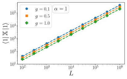
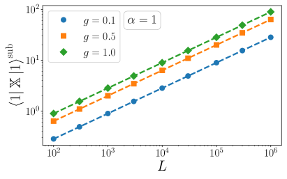
Figure 10: Finite-size scaling of $\chi_{A}^{x}:=\langle 1|\mathbb{X}|1\rangle$ in the ferromagnetic phase of the quantum spherical model with long-range interactions. In the figure we plot $\langle 1|\mathbb{X}|1\rangle_{A}$ versus $L$. Notice the logarithmic scale on both axes. (Top row). Results for $\alpha=1$. In the left panel we focus on the the leading scaling behavior in the large $L$ limit. The different symbols correspond to different values of $g$. The lines are the analytic results (first term in (32)). The right panel shows the first subleading term $\langle 1|\mathbb{X}|1\rangle_{A}^{\mathrm{sub}}$ of $\left<1\right|\mathbb{X}\left|1\right>$. The data are obtained from those in the left panel by subtracting the analytic prediction for the leading behavior. The dashed line are the analytic results (second term in (32)). (Bottom row). The same as in the top row for $\alpha=1.5$.

Appendix D Finite-size scaling of the susceptibility $\chi_{A}^{t}$

Here we derive the flat-vector expectation values of the momentum correlation matrix $\langle 1|\mathbb{P}|1\rangle_{A}$, i.e., of the susceptibility $\chi_{A}^{t}$. The correlation matrix $\mathbb{P}_{nm}$ reads (see Eq. (11b))

$$\mathbb{P}_{nm}=\frac{1}{\sqrt{g}}\frac{1}{2L}\sum_{k=0}^{L-1}e^{\mathrm{i}(n-m)\frac{2\pi}{L}k}\sqrt{2\mu+\omega_{k}},$$ (98)

with the frequency $\omega_{k}$ defined as in (3). Again, we use Poisson’s summation formula (43) to split (98) into a thermodynamic and a finite-size part, i.e., $\mathbb{P}_{nm}=\mathbb{P}^{\rm(th)}_{nm}+\mathbb{P}^{\rm(L)}_{nm}$. Specifically, we have

$$\mathbb{P}^{\rm(th)}_{nm} =\frac{1}{2}\frac{1}{\sqrt{g}}\int_{0}^{2\pi}\frac{\mathrm{d}k}{2\pi}e^{\mathrm{i}(n-m)k}\sqrt{2\mu+\omega_{k}},$$ (99)

$$\mathbb{P}^{\rm(L)}_{nm} =\frac{1}{\sqrt{g}}\sum_{j=1}^{\infty}\int_{0}^{2\pi}\frac{\mathrm{d}k}{2\pi}e^{\mathrm{i}(n-m)k}\cos\left(Ljk\right)\sqrt{2\mu+\omega_{k}}.$$ (100)

We consider a bipartition of the chain into two parts as $A\cup B$, with $B$ the complement of $A$. We denote the size of $A$ as $L_{A}$ and proceed to compute the flat-vector expectation value of the momentum correlation matrix

$$\chi_{A}^{t}=\langle 1|\mathbb{P}|1\rangle_{A}:=\frac{1}{L_{A}}\sum_{n,m=0}^{L_{A}-1}\mathbb{P}_{nm}.$$ (101)

In the following we consider $L_{A}=L/2$ and treat the thermodynamic and the finite-size contributions separately.

D.1 A useful integral

In order to extract the finite-size scaling of $\bra{1}\mathbb{P}\ket{1}_{A}$ we need to analyze the “universal” part of the integral

$$\mathfrak{J}(s)=\int_{0}^{2\pi}\frac{\mathrm{d}k}{2\pi}k^{-s}\sqrt{2\mu+\omega(k)}.$$ (102)

Hence, it suffices to consider the small $k$ limit and study $\mu\to 0$. To this end, we introduce a cutoff $\Lambda$ as follows

$$\mathfrak{J}(s)\simeq\int_{0}^{\Lambda}\frac{\mathrm{d}k}{\pi}k^{-s}\sqrt{2\mu+\omega(k)}=\frac{1}{\pi}\frac{\Lambda^{1-s}}{1-s}\sqrt{2\mu}+\int_{0}^{\Lambda}\frac{\mathrm{d}k}{\pi}k^{-s}\left(\sqrt{2\mu+\omega(k)}-\sqrt{2\mu}\right).$$ (103)

After using the short wavelength approximation and after changing variable as $y^{2}=k^{\alpha}/(2\mu)$, we obtain

$$\mathfrak{J}(s)\simeq\frac{1}{\pi}\frac{\Lambda^{1-s}}{1-s}\sqrt{2\mu}+\frac{2}{\alpha}\int_{0}^{\sqrt{\Lambda^{\alpha}/2\mu}}\frac{\mathrm{d}y}{\pi}y^{\frac{2}{\alpha}(1-s)-1}\left(\sqrt{1+y^{2}}-1\right)(2\mu)^{\frac{1}{2}+\frac{1-s}{\alpha}}\\ \simeq\frac{2}{\alpha}(2\mu)^{\frac{1}{2}+\frac{1-s}{\alpha}}\int_{0}^{\infty}\frac{\mathrm{d}y}{\pi}y^{\frac{2}{\alpha}(1-s)-1}\left(\sqrt{1+y^{2}}-1\right)$$ (104)

where we took the limit $\mu\to 0$, we neglected all cutoff-dependent contributions and we multiplied by two the result to account for the singularities. The remaining integral is readily evaluated, and we find for $1+\alpha/2<\operatorname{Re}(s)<1+\alpha$

$$\mathfrak{J}\simeq-\frac{\pi^{-3/2}}{2\alpha}(2\mu)^{\frac{1}{2}+\frac{1-s}{\alpha}}\Gamma\left(-\frac{1}{2}-\frac{1-s}{\alpha}\right)\Gamma\left(\frac{1-s}{\alpha}\right).$$ (105)

Eq. (105) contains full information about the universal contributions at criticality. One should observe that the leading behavior of thermodynamic contribution $\langle 1|\mathbb{P}^{\mathrm{(th)}}|1\rangle_{A}$ in the large $L$ limit is not “universal”, meaning that it depends on the cutoff $\Lambda$. Cutoff-independent terms are subleading. This is in contrast with $\chi_{A}^{x}$ (see C).

D.2 Thermodynamic contribution

As in C, we again observe that Eq. (99) only depends on the difference $n-m$ and thus, we can rewrite it using Eq. (71) as

$$\bra{1}\mathbb{P}^{\rm(th)}\ket{1}_{A}=\frac{1}{\sqrt{g}}\int_{0}^{2\pi}\frac{\mathrm{d}k}{2\pi}\sqrt{2\mu+\omega_{k}}\left[\frac{1}{2}+\sum_{n=1}^{L/2}\cos(kn)\left(1-\frac{2n}{L}\right)\right].$$ (106)

As for $\chi_{A}^{x}$, we shall treat the three contributions in the bracket separately. For the first contribution in (106) we find

$$\frac{1}{2}\int_{0}^{2\pi}\frac{\mathrm{d}k}{2\pi}\sqrt{2\mu+\omega_{k}}\simeq A+B\cdot(2\mu)+C\cdot(2\mu)^{\frac{1}{2}+1/\alpha},$$ (107)

with

$$A =\int_{0}^{2\pi}\frac{\mathrm{d}k}{4\pi}\sqrt{\omega_{k}}=2^{\frac{\alpha}{2}-1}\frac{\Gamma((2+\alpha)/4)}{\sqrt{\pi}\Gamma(1+\alpha/4)}$$ (108)

$$B =\int_{0}^{2\pi}\frac{\mathrm{d}k}{8\pi}\frac{1}{\sqrt{\omega_{k}}}=2^{-2-\frac{\alpha}{2}}\frac{\Gamma((2-\alpha)/4)}{\sqrt{\pi}\Gamma(1-\alpha/4)}$$ (109)

$$C =-\frac{\pi^{-3/2}}{4\alpha}\Gamma\left(-\frac{1}{2}-\frac{1}{\alpha}\right)\Gamma\left(\frac{1}{\alpha}\right)$$ (110)

In deriving (107) we expanded the integrand for $\mu\to 0$, keeping only terms up to ${\mathcal{O}}(\mu)$. This gives the first two terms in (107). As it is clear from (108) and (109) the prefactors $A$ and $B$ depend on the full dispersion $\omega_{k}$, and hence on the cutoff $\Lambda$. This means that the first tow contributions in (107) are not “universal”. The last term in (107) is obtained from (105) by fixing $s=0$. This last term depends only on the low-energy part of the dispersion, and hence is “universal”.

Let us now evaluate the second contribution $T_{1}$ in (106), i.e.,

$$T_{1}=\sum_{r=1}^{L/2}\int_{0}^{2\pi}\frac{\mathrm{d}k}{2\pi}\sqrt{2\mu+\omega_{k}}\cos(kr).$$ (111)

Here we omit the $1/\sqrt{g}$ as compared with (106). To evaluate (111) we use the Mellin technique as in C. To this end we use the identity

$$\cos(x)=\int_{\gamma}\frac{\mathrm{d}s}{2\pi\mathrm{i}}x^{-s}\cos\left(\frac{\pi}{2}s\right)\Gamma(s),$$ (112)

Here $\gamma$ denotes a contour in the complex plane enclosing the entire negative real axis, and not exceeding $\mathrm{Re}(s)=1$. Thus, Eq. (112) can be verified by using Cauchy’s residue theorem. After carrying out the sum over $r$ in (111), and subsequently expanding the harmonic numbers for $L\to\infty$ yields

$$T_{1}\simeq\int_{\gamma}\frac{\mathrm{d}s}{2\pi\mathrm{i}}\left(\frac{L}{2}\right)^{1-s}\frac{\cos\left(\pi s/2\right)}{1-s}\Gamma(s)\mathfrak{J}(s),$$ (113)

where $\mathfrak{J}(s)$ is the integral in (102). Since the pole at $s=1$ in (113) is removed by the vanishing of the cosine, we can deform the path $\gamma$ into a new path $\gamma^{\prime}$ that still encloses the entire negative axis but closes such that $1+\alpha/2<\operatorname{Re}(s)<1+\alpha$. Now, we can use the expression in Eq. (105) to obtain

$$T_{1}\simeq-\frac{\pi^{-\frac{3}{2}}}{2\alpha}\int_{\gamma^{\prime}}\frac{\mathrm{d}s}{2\pi\mathrm{i}}\left(\frac{L}{2}\right)^{1-s}(2\mu)^{\frac{1}{2}+\frac{1-s}{\alpha}}\frac{\cos\left(\pi s/2\right)}{1-s}\Gamma(s)\Gamma\left(-\frac{1}{2}-\frac{1-s}{\alpha}\right)\Gamma\left(\frac{1-s}{\alpha}\right).$$ (114)

The leading contribution to $T_{1}$ is readily found from the residue at $s=1+\alpha/2$, i.e.,

$$T_{1}\simeq\frac{2^{1+\frac{\alpha}{2}}}{\alpha\pi}\sin\left(\frac{\pi}{4}\alpha\right)\Gamma\left(1+\frac{\alpha}{2}\right)L^{-\frac{\alpha}{2}}.$$ (115)

Subleading contributions can be found from the remaining residues of the integrand in (114). A similar procedure allows us to evaluate the last contribution in (106), i.e.,

$$T_{2}=\frac{2}{L}\sum_{n=1}^{L/2}\int_{0}^{2\pi}\frac{\mathrm{d}k}{2\pi}n\cos(nk)\sqrt{2\mu+\omega(k)}\\ \simeq\frac{\pi^{-\frac{3}{2}}}{2\alpha}\int_{\gamma^{\prime}}\frac{\mathrm{d}s}{2\pi\mathrm{i}}\left(\frac{L}{2}\right)^{1-s}(2\mu)^{\frac{1}{2}+\frac{1-s}{\alpha}}\frac{\cos\left(\pi s/2\right)}{s-2}\Gamma(s)\Gamma\left(-\frac{1}{2}-\frac{1-s}{\alpha}\right)\Gamma\left(\frac{1-s}{\alpha}\right).$$ (116)

Again, the leading contribution comes from the pole at $s=1+\alpha/2$ and we find

$$T_{2}\simeq-\frac{2^{\frac{\alpha}{2}+1}}{\pi}\frac{\sin\left(\pi\alpha/4\right)}{2-\alpha}\Gamma\left(1+\frac{\alpha}{2}\right)L^{-\frac{\alpha}{2}}.$$ (117)

Finally, by putting together (115) and (117) we obtain the result for $\langle 1|\mathbb{P}^{\mathrm{(th)}}|1\rangle_{A}$ as

$$\bra{1}\mathbb{P}^{({\rm th})}\ket{1}_{A}\simeq\frac{2^{1+\frac{\alpha}{2}}}{\pi\sqrt{g}}\sin\left(\frac{\pi}{4}\alpha\right)\Gamma\left(1+\frac{\alpha}{2}\right)\frac{2}{\alpha(2-\alpha)}L^{-\frac{\alpha}{2}}.$$ (118)

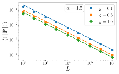
Figure 11: Finite-size scaling behavior of $\chi_{A}^{t}=\langle 1|\mathbb{P}|1\rangle_{A}$ in the ordered phase of the QSM with long-range interactions. We plot $\chi_{A}^{t}$ versus $L$. Notice the logarithmic scale on both axes. The different panels correspond to different values of the exponent $\alpha$ of the long-range interactions. In each figure different symbols correspond to different values of $g$. The lines are the theory predictions obtained summing (118) and (123).

D.3 Finite-size contribution

Let us now determine the scaling behavior of the finite-size contribution $\langle 1|\mathbb{P}^{\mathrm{(L)}}|1\rangle_{A}$ (cf. (100)). Specifically, here we have to evaluate a term $T_{3}$ of the form

$$T_{3}=\frac{2}{L}\sum_{j=1}^{\infty}\sum_{n,m=0}^{L/2}e^{\mathrm{i}(n-m)k}\cos(Ljk)\sqrt{2\mu+\omega(k)}.$$ (119)

First, we express $\cos(Ljk)$ in terms of complex exponentials, and use the representation

$$e^{\mathrm{i}kx}=\int_{\gamma}\frac{\mathrm{d}s}{2\pi\mathrm{i}}(-\mathrm{i}x)^{-s}\Gamma(s),$$ (120)

which is the analog of (112). Again, the path $\gamma$ is chosen as in (112), and it encloses the whole negative real axis. Subsequently, we exploit that the double sum in (119) only depends on $n-m$. We can use (71) and (102) to obtain

$$T_{3}=\frac{1}{2}\sum_{j=1}^{\infty}\sum_{q=-L/2}^{L/2}\int_{\gamma}\frac{\mathrm{d}s}{2\pi\mathrm{i}}\Gamma(s)\frac{(-\mathrm{i})^{s}}{(q\pm Lj)^{s}}\left(1-\frac{2}{L}|q|\right)\mathfrak{J}(s),$$ (121)

where one has to sum over the $\pm$. We can neglect the term with $q=0$ in (121) because it is subleading. We can also combine the contributions for $q$ and $-q$ in the sum. After using the same contour $\gamma^{\prime}$ as in (114), and after performing the sum over $j$, we obtain

$$T_{3}\simeq\sum_{q=1}^{L/2}\int_{\gamma}\frac{\mathrm{d}s}{2\pi\mathrm{i}}\Gamma(s)\cos\left(\frac{\pi}{2}s\right)L^{-s}\zeta\left(s,1\pm\frac{q}{L}\right)\left(1-\frac{2}{L}|q|\right)\mathfrak{J}(s).$$ (122)

Again, the leading scaling behavior in the limit $L\to\infty$ is given by the residue at $s=1+\alpha/2$. We obtain

$$\langle 1|\mathbb{P}^{\rm(L)}|1\rangle_{A}\simeq\Gamma\left(1+\frac{\alpha}{2}\right)\cos\left(1+\frac{\alpha}{2}\right)\int_{0}^{1}(1-x)\zeta\left(1+\frac{\alpha}{2},1\pm\frac{x}{2}\right)\frac{\mathrm{d}x}{2\pi}L^{-\frac{\alpha}{2}}$$ (123)

where one has to sum over the signs in the argument of the Hurwitz zeta function, and we replaced the sum over $q$ with an integral. Importantly, the finite size contribution to $\chi_{A}^{t}$ is ${\mathcal{O}}(L^{-\alpha/2})$, as the thermodynamic one (cf. (118)).

References

References

- [1] Amico L, Fazio R, Osterloh A and Vedral V 2008 Rev. Mod. Phys. 80(2) 517–576 URL https://link.aps.org/doi/10.1103/RevModPhys.80.517
- [2] Eisert J, Cramer M and Plenio M B 2010 Rev. Mod. Phys. 82(1) 277–306 URL https://link.aps.org/doi/10.1103/RevModPhys.82.277
- [3] Calabrese P, Cardy J and Doyon B 2009 Journal of Physics A: Mathematical and Theoretical 42 500301 URL https://doi.org/10.1088/1751-8121/42/50/500301
- [4] Laflorencie N 2016 Physics Reports 646 1–59 URL https://doi.org/10.1016/j.physrep.2016.06.008
- [5] White S R 1992 Phys. Rev. Lett. 69(19) 2863–2866 URL https://link.aps.org/doi/10.1103/PhysRevLett.69.2863
- [6] Peschel I, Kaulke M and Legeza O 1999 Annalen der Physik 8 153–164
- [7] Peschel I 2004 Journal of Statistical Mechanics: Theory and Experiment 2004 P06004 URL https://doi.org/10.1088/1742-5468/2004/06/p06004
- [8] Thomale R, Arovas D P and Bernevig B A 2010 Phys. Rev. Lett. 105(11) 116805 URL https://link.aps.org/doi/10.1103/PhysRevLett.105.116805
- [9] Läuchli A M, Bergholtz E J, Suorsa J and Haque M 2010 Phys. Rev. Lett. 104(15) 156404 URL https://link.aps.org/doi/10.1103/PhysRevLett.104.156404
- [10] Haque M, Zozulya O and Schoutens K 2007 Phys. Rev. Lett. 98(6) 060401 URL https://link.aps.org/doi/10.1103/PhysRevLett.98.060401
- [11] Thomale R, Sterdyniak A, Regnault N and Bernevig B A 2010 Phys. Rev. Lett. 104(18) 180502 URL https://link.aps.org/doi/10.1103/PhysRevLett.104.180502
- [12] Hermanns M, Chandran A, Regnault N and Bernevig B A 2011 Phys. Rev. B 84(12) 121309(R) URL https://link.aps.org/doi/10.1103/PhysRevB.84.121309
- [13] Chandran A, Hermanns M, Regnault N and Bernevig B A 2011 Phys. Rev. B 84(20) 205136 URL https://link.aps.org/doi/10.1103/PhysRevB.84.205136
- [14] Qi X L, Katsura H and Ludwig A W W 2012 Phys. Rev. Lett. 108(19) 196402 URL https://link.aps.org/doi/10.1103/PhysRevLett.108.196402
- [15] Liu Z, Bergholtz E J, Fan H and Läuchli A M 2012 Phys. Rev. B 85(4) 045119 URL https://link.aps.org/doi/10.1103/PhysRevB.85.045119
- [16] Sterdyniak A, Chandran A, Regnault N, Bernevig B A and Bonderson P 2012 Phys. Rev. B 85(12) 125308 URL https://link.aps.org/doi/10.1103/PhysRevB.85.125308
- [17] Dubail J, Read N and Rezayi E H 2012 Phys. Rev. B 85(11) 115321 URL https://link.aps.org/doi/10.1103/PhysRevB.85.115321
- [18] Dubail J, Read N and Rezayi E H 2012 Phys. Rev. B 86(24) 245310 URL https://link.aps.org/doi/10.1103/PhysRevB.86.245310
- [19] Chandran A, Khemani V and Sondhi S L 2014 Phys. Rev. Lett. 113(6) 060501 URL https://link.aps.org/doi/10.1103/PhysRevLett.113.060501
- [20] Pollmann F, Turner A M, Berg E and Oshikawa M 2010 Phys. Rev. B 81(6) 064439 URL https://link.aps.org/doi/10.1103/PhysRevB.81.064439
- [21] Turner A M, Pollmann F and Berg E 2011 Phys. Rev. B 83(7) 075102 URL https://link.aps.org/doi/10.1103/PhysRevB.83.075102
- [22] Bauer B, Cincio L, Keller B, Dolfi M, Vidal G, Trebst S and Ludwig A 2014 Nature Communications 5 URL https://doi.org/10.1038/ncomms6137
- [23] Poilblanc D 2010 Phys. Rev. Lett. 105(7) 077202 URL https://link.aps.org/doi/10.1103/PhysRevLett.105.077202
- [24] Cirac J I, Poilblanc D, Schuch N and Verstraete F 2011 Phys. Rev. B 83(24) 245134 URL https://link.aps.org/doi/10.1103/PhysRevB.83.245134
- [25] De Chiara G, Lepori L, Lewenstein M and Sanpera A 2012 Phys. Rev. Lett. 109(23) 237208 URL https://link.aps.org/doi/10.1103/PhysRevLett.109.237208
- [26] Alba V, Haque M and Läuchli A M 2012 Phys. Rev. Lett. 108(22) 227201 URL https://link.aps.org/doi/10.1103/PhysRevLett.108.227201
- [27] Metlitski M A and Grover T 2011 Entanglement entropy of systems with spontaneously broken continuous symmetry (Preprint arXiv:1112.5166)
- [28] Alba V, Haque M and Läuchli A M 2012 Journal of Statistical Mechanics: Theory and Experiment 2012 P08011 URL https://doi.org/10.1088/1742-5468/2012/08/p08011
- [29] Alba V, Haque M and Läuchli A M 2013 Phys. Rev. Lett. 110(26) 260403 URL https://link.aps.org/doi/10.1103/PhysRevLett.110.260403
- [30] Lepori L, De Chiara G and Sanpera A 2013 Phys. Rev. B 87(23) 235107 URL https://link.aps.org/doi/10.1103/PhysRevB.87.235107
- [31] James A J A and Konik R M 2013 Phys. Rev. B 87(24) 241103 URL https://link.aps.org/doi/10.1103/PhysRevB.87.241103
- [32] Kolley F, Depenbrock S, McCulloch I P, Schollwöck U and Alba V 2013 Phys. Rev. B 88(14) 144426 URL https://link.aps.org/doi/10.1103/PhysRevB.88.144426
- [33] Rademaker L 2015 Phys. Rev. B 92(14) 144419 URL https://link.aps.org/doi/10.1103/PhysRevB.92.144419
- [34] Kolley F, Depenbrock S, McCulloch I P, Schollwöck U and Alba V 2015 Phys. Rev. B 91(10) 104418 URL https://link.aps.org/doi/10.1103/PhysRevB.91.104418
- [35] Frérot I and Roscilde T 2016 Phys. Rev. Lett. 116(19) 190401 URL https://link.aps.org/doi/10.1103/PhysRevLett.116.190401
- [36] Alba V 2021 SciPost Phys. 10 056 URL https://scipost.org/10.21468/SciPostPhys.10.3.056
- [37] Contessi D, Recati A and Rizzi M 2022 Phase Diagram Detection via Gaussian Fitting of Number Probability Distribution URL https://arxiv.org/abs/2207.01478
- [38] Bayat A, Johannesson H, Bose S and Sodano P 2014 Nature Communications 5 URL https://doi.org/10.1038/ncomms4784
- [39] Calabrese P and Lefevre A 2008 Phys. Rev. A 78(3) 032329 URL https://link.aps.org/doi/10.1103/PhysRevA.78.032329
- [40] Läuchli A M 2013 Operator content of real-space entanglement spectra at conformal critical points (Preprint arXiv:1303.0741)
- [41] Alba V, Calabrese P and Tonni E 2017 Journal of Physics A: Mathematical and Theoretical 51 024001 URL https://doi.org/10.1088%2F1751-8121%2Faa9365
- [42] Cardy J 2015 The entanglement gap in cfts, talk at the kitp conference ”closing the entanglement gap: Quantum information, quantum matter, and quantum fields”. URL http://online.kitp.ucsb.edu/online/entangled-c15/cardy/
- [43] Ruggiero P, Alba V and Calabrese P 2016 Phys. Rev. B 94(19) 195121 URL https://link.aps.org/doi/10.1103/PhysRevB.94.195121
- [44] Defenu N, Donner T, Macrì T, Pagano G, Ruffo S and Trombettoni A 2021 Long-range interacting quantum systems URL https://arxiv.org/abs/2109.01063
- [45] Zhang J, Pagano G, Hess P W, Kyprianidis A, Becker P, Kaplan H, Gorshkov A V, Gong Z X and Monroe C 2017 Nature 551 601–604 ISSN 1476-4687 URL https://doi.org/10.1038/nature24654
- [46] Koffel T, Lewenstein M and Tagliacozzo L 2012 Phys. Rev. Lett. 109(26) 267203 URL https://link.aps.org/doi/10.1103/PhysRevLett.109.267203
- [47] Nezhadhaghighi M G and Rajabpour M A 2013 Phys. Rev. B 88(4) 045426 URL https://link.aps.org/doi/10.1103/PhysRevB.88.045426
- [48] Vodola D, Lepori L, Ercolessi E and Pupillo G 2015 New Journal of Physics 18 015001 URL https://dx.doi.org/10.1088/1367-2630/18/1/015001
- [49] Frérot I, Naldesi P and Roscilde T 2017 Phys. Rev. B 95(24) 245111 URL https://link.aps.org/doi/10.1103/PhysRevB.95.245111
- [50] Gong Z X, Foss-Feig M, Brandão F G S L and Gorshkov A V 2017 Phys. Rev. Lett. 119(5) 050501 URL https://link.aps.org/doi/10.1103/PhysRevLett.119.050501
- [51] Mohammadi Mozaffar M R and Mollabashi A 2017 Journal of High Energy Physics 2017 120 ISSN 1029-8479 URL https://doi.org/10.1007/JHEP07(2017)120
- [52] Maghrebi M F, Gong Z X and Gorshkov A V 2017 Phys. Rev. Lett. 119(2) 023001 URL https://link.aps.org/doi/10.1103/PhysRevLett.119.023001
- [53] Pappalardi S, Russomanno A, Žunkovič B, Iemini F, Silva A and Fazio R 2018 Phys. Rev. B 98(13) 134303 URL https://link.aps.org/doi/10.1103/PhysRevB.98.134303
- [54] Mozaffar M R M and Mollabashi A 2019 Journal of High Energy Physics 2019 137 ISSN 1029-8479 URL https://doi.org/10.1007/JHEP01(2019)137
- [55] Bentsen G S, Daley A J and Schachenmayer J 2022 Entanglement Dynamics in Spin Chains with Structured Long-Range Interactions (Cham: Springer International Publishing) pp 285–319 ISBN 978-3-031-03998-0 URL https://doi.org/10.1007/978-3-031-03998-0_11
- [56] Ares F, Murciano S and Calabrese P 2022 Journal of Statistical Mechanics: Theory and Experiment 2022 063104 URL https://dx.doi.org/10.1088/1742-5468/ac7644
- [57] Truong T T and Peschel I 1989 Zeitschrift für Physik B Condensed Matter 75 119–125 URL https://doi.org/10.1007/bf01313574
- [58] Chung M C and Peschel I 2000 Phys. Rev. B 62(7) 4191–4193 URL https://link.aps.org/doi/10.1103/PhysRevB.62.4191
- [59] Giulio G D and Tonni E 2020 Journal of Statistical Mechanics: Theory and Experiment 2020 033102 URL https://doi.org/10.1088/1742-5468/ab7129
- [60] Lhuillier C and Misguich G 2002 Frustrated quantum magnets High Magnetic Fields (Springer Berlin Heidelberg) pp 161–190 URL https://doi.org/10.1007/3-540-45649-x_6
- [61] Beekman A J, Rademaker L and van Wezel J 2019 SciPost Phys. Lect. Notes 11 URL https://scipost.org/10.21468/SciPostPhysLectNotes.11
- [62] Wietek A, Schuler M and Läuchli A M 2017 Studying continuous symmetry breaking using energy level spectroscopy (Preprint 1704.08622)
- [63] Lundgren R, Blair J, Greiter M, Läuchli A, Fiete G A and Thomale R 2014 Phys. Rev. Lett. 113(25) 256404 URL https://link.aps.org/doi/10.1103/PhysRevLett.113.256404
- [64] Obermair G 1972 A dynamical spherical model Dynamical Aspects of critical phenomena (New York: Gordon and Breach) p 10
- [65] Henkel M and Hoeger C 1984 Zeitschrift für Physik B Condensed Matter 55 67–73 ISSN 0722-3277 URL http://link.springer.com/10.1007/BF01307503
- [66] Vojta T 1996 Physical Review B 53 710 ISSN 0163-1829 URL http://link.aps.org/abstract/PRB/v53/p710{%}5Cnpapers2://publication/uuid/A5F04936-25CE-4C76-906D-78E3C75CD931
- [67] Wald S and Henkel M 2015 Journal of Statistical Mechanics: Theory and Experiment 07006 34 ISSN 17425468 (Preprint 1503.06713) URL http://arxiv.org/abs/1503.06713
- [68] Wald S, Arias R and Alba V 2020 Phys. Rev. Research 2(4) 043404 URL https://link.aps.org/doi/10.1103/PhysRevResearch.2.043404
- [69] Berlin T H and Kac M 1952 Physical Review 86 821–835 ISSN 0031-899X URL https://link.aps.org/doi/10.1103/PhysRev.86.821
- [70] Pelissetto A and Vicari E 2002 Physics Reports 368 549–727 URL https://doi.org/10.1016/s0370-1573(02)00219-3
- [71] Zinn-Justin J 1998 Vector models in the large limit: a few applications (Preprint arXiv:hep-th/9810198)
- [72] Stanley H E 1968 Phys. Rev. 176(2) 718–722 URL https://link.aps.org/doi/10.1103/PhysRev.176.718
- [73] Metlitski M A, Fuertes C A and Sachdev S 2009 Phys. Rev. B 80(11) 115122 URL https://link.aps.org/doi/10.1103/PhysRevB.80.115122
- [74] Whitsitt S, Witczak-Krempa W and Sachdev S 2017 Phys. Rev. B 95(4) 045148 URL https://link.aps.org/doi/10.1103/PhysRevB.95.045148
- [75] Lu T C and Grover T 2019 Physical Review B 99 075157 ISSN 2469-9950 (Preprint 1808.04381) URL https://arxiv.org/pdf/1808.04381.pdfhttp://arxiv.org/abs/1808.04381http://dx.doi.org/10.1103/PhysRevB.99.075157https://link.aps.org/doi/10.1103/PhysRevB.99.075157
- [76] Lu T C and Grover T 2019 Structure of quantum entanglement at a finite temperature critical point (Preprint 1907.01569)
- [77] Wald S, Arias R and Alba V 2020 Journal of Statistical Mechanics: Theory and Experiment 2020 033105 URL https://doi.org/10.1088%2F1742-5468%2Fab6b19
- [78] Zoia A, Rosso A and Kardar M 2007 Phys. Rev. E 76(2) 021116 URL https://link.aps.org/doi/10.1103/PhysRevE.76.021116
- [79] Bienzobaz P and Salinas S 2012 Physica A: Statistical Mechanics and its Applications 391 6399 – 6408 ISSN 0378-4371 URL http://www.sciencedirect.com/science/article/pii/S0378437112006929
- [80] Peschel I and Eisler V 2009 Journal of Physics A: Mathematical and Theoretical 42 504003 URL https://doi.org/10.1088/1751-8113/42/50/504003
- [81] Botero A and Reznik B 2004 Phys. Rev. A 70(5) 052329 URL https://link.aps.org/doi/10.1103/PhysRevA.70.052329
- [82] Kosterlitz J M, Thouless D J and Jones R C 1976 Phys. Rev. Lett. 36(20) 1217–1220 URL https://link.aps.org/doi/10.1103/PhysRevLett.36.1217
- [83] Hornreich R M and Schuster H G 1982 Phys. Rev. B 26(7) 3929–3936 URL https://link.aps.org/doi/10.1103/PhysRevB.26.3929
- [84] Jagannathan A and Rudnick J 1989 Journal of Physics A: Mathematical and General 22 5131–5141 URL https://doi.org/10.1088%2F0305-4470%2F22%2F23%2F017
- [85] Vojta T 1993 Journal of Physics A: Mathematical and General 26 2883–2893 URL https://doi.org/10.1088%2F0305-4470%2F26%2F12%2F025
- [86] Vojta T and Schreiber M 1996 Phys. Rev. B 53(13) 8211–8214 URL https://link.aps.org/doi/10.1103/PhysRevB.53.8211
- [87] Chandran A, Nanduri A, Gubser S S and Sondhi S L 2013 Phys. Rev. B 88(2) 024306 URL https://link.aps.org/doi/10.1103/PhysRevB.88.024306
- [88] Barbier D, Cugliandolo L F, Lozano G S, Nessi N, Picco M and Tartaglia A 2019 Journal of Physics A: Mathematical and Theoretical 52 454002 URL https://dx.doi.org/10.1088/1751-8121/ab3ff1
- [89] Barbier D, Cugliandolo L F, Lozano G S and Nessi N 2022 SciPost Phys. 13 048 URL https://scipost.org/10.21468/SciPostPhys.13.3.048
- [90] Henkel M 2022 Quantum dynamics far from equilibrium: a case study in the spherical model URL https://arxiv.org/abs/2201.06448
- [91] Shapourian H, Ruggiero P, Ryu S and Calabrese P 2019 SciPost Phys. 7(3) 37 URL https://scipost.org/10.21468/SciPostPhys.7.3.037
- [92] Turkeshi X, Ruggiero P and Calabrese P 2020 Phys. Rev. B 101(6) 064207 URL https://link.aps.org/doi/10.1103/PhysRevB.101.064207
- [93] Brankov J G and Tonchev N S 1988 Journal of Statistical Physics 52 143–159 ISSN 1572-9613 URL https://doi.org/10.1007/BF01016408
- [94] NIST Digital Library of Mathematical Functions http://dlmf.nist.gov/, Release 1.1.7 of 2022-10-15 f. W. J. Olver, A. B. Olde Daalhuis, D. W. Lozier, B. I. Schneider, R. F. Boisvert, C. W. Clark, B. R. Miller, B. V. Saunders, H. S. Cohl, and M. A. McClain, eds. URL http://dlmf.nist.gov/
- [95] Contino R and Gambassi A 2003 Journal of Mathematical Physics 44 570 URL https://doi.org/10.1063/1.1531215