Quantum phase transition in the spin-anisotropic quantum spherical model

Sascha Wald and Malte Henkel

Groupe de Physique Statistique,

Département de Physique de la Matière et des Matériaux,

Institut Jean Lamour (CNRS UMR 7198), Université de Lorraine Nancy,

B.P. 70239, F – 54506 Vandœuvre lès Nancy Cedex, France

Motivated by an analogy with the spin anisotropies in the quantum XY chain and its reformulation in terms of spin-less Majorana fermions, its bosonic analogue, the spin-anisotropic quantum spherical model, is introduced. The exact solution of the model permits to analyse the influence of the spin-anisotropy on the phase diagram and the universality of the critical behaviour in a new way, since the interactions of the quantum spins and their conjugate momenta create new effects. At zero temperature, a quantum critical line is found, which is in the same universality class as the thermal phase transition in the classical spherical model in $d+1$ dimensions. The location of this quantum critical line shows a re-entrant quantum phase transition for dimensions $1<d\lesssim 2.065$.

PACS numbers: 05.30.-d, 05.30.Jp, 05.30.Rt, 64.60.De, 64.60.F-
 

1 Introduction

The study of equilibrium phase transitions has taken enormous benefits from the analysis of exactly solvable models [45, 7, 39, 62, 11, 13]. The classical spherical model, invented in the seminal work by Berlin and Kac [8] and with its subsequent simplification by Lewis and Wannier [52], has been a valuable test system for the explicit analytical verification of more general scaling descriptions, in a specific setting (examples are critical behaviour of observables or finite-size scaling). It is related with more realistic spin systems as the $n\to\infty$ limit of the ${\rm O}(n)$-symmetric Heisenberg model [66]. It is well-known, as already observed by Berlin and Kac [8], that in the original formulation in terms of classical spin variables $S_{i}\in\mathbb{R}$, the specific heat does not vanish in the zero-temperature limit, hence the Nernst theorem is not obeyed in this model. This was one motivation to take the quantum nature of the spin variables into account, by a canonical quantisation scheme, and has lead to Obermair’s formulation of the quantum spherical model [57]. This takes the form of a quantum rotor model, where the kinetic energy term in the hamiltonian does not commute with the spin-exchange interactions. The properties of this exactly solvable model have been analysed in great detail, see e.g. [57, 64, 56, 68, 18, 62, 11, 32, 58, 9, 10]. Independently, the quantum spherical model was also obtained via the so-called ‘hamiltonian limit’ [50] as the logarithm of the transfer matrix in an extremely anisotropic limit [65, 35, 38]. In its most conventional formulation as a quantum rotor model [57, 35, 68], the quantum spherical model may be obtained as the limit $n\to\infty$ of the quantum non-linear O($n$) sigma-model [68]. For different choices of the kinetic energy term, there are further quantum spherical models, which become the $n\to\infty$ limit of an SU($n$) Heisenberg ferromagnet or anti-ferromagnet [56, 32].

Quantum spherical models have been discussed in the context of specific applications, for example for the description of networks of Josephson-junction arrays [27, 16]. Certain modern theories of cuprate supraconductivity are based on SO(5)-symmetric quantum non-linear sigma models, and it is thought that this kind of models might be an effective description of the large-distance, low-energy properties of more realistic models, see e.g. [22] for a detailed review.

Habitually, (mean) spherical models are defined in terms of a classical hamiltonian

$${\cal H}_{\rm cl}=\sum_{\boldsymbol{n}}\left[-J\sum_{j=1}^{d}{S}_{\boldsymbol{n}}{S}_{\boldsymbol{n}+\boldsymbol{e}_{j}}-BS_{\boldsymbol{n}}+\frac{\mu}{2}{S}_{\boldsymbol{n}}^{2}\right]$$ (1.1)

with the spherical spins ${S}_{\boldsymbol{n}}\in\mathbb{R}$. Herein, $\boldsymbol{n}$ runs over the sites of a $d$-dimensional hyper-cubic lattice with ${\cal N}=N^{d}$ sites, the vectors $\boldsymbol{e}_{j}$, $1\leq j\leq d$, are the unit vectors in the $j^{\rm th}$ direction, $B$ is an external magnetic field and $J$ is the exchange integral. Finally, the spherical spins obey the mean ‘spherical constraint’ $\sum_{\boldsymbol{n}}\left\langle S_{\boldsymbol{n}}^{2}\right\rangle\stackrel{{\scriptstyle!}}{{=}}{\cal N}$ [8, 52], from which $\mu$ is found.

The generalisation towards a quantum spherical model is formulated by considering now the spins $S_{\boldsymbol{n}}\mapsto\widehat{S}_{\boldsymbol{n}}$ as operators, and introducing canonically conjugate momenta $\widehat{P}_{\boldsymbol{n}}$, which obey the canonical commutation relations

$$\left[\widehat{S}_{\boldsymbol{n}},\widehat{P}_{\boldsymbol{m}}\right]={\rm i}\hbar\,\delta_{\boldsymbol{n},\boldsymbol{m}}\;\;,\;\;\left[\widehat{S}_{\boldsymbol{n}},\widehat{S}_{\boldsymbol{m}}\right]=\left[\widehat{P}_{\boldsymbol{n}},\widehat{P}_{\boldsymbol{m}}\right]=0$$ (1.2)

The most common ansatz for the quantum hamiltonian is to make ${\cal H}_{\rm cl}\mapsto\widehat{H}_{\rm cl}$ an operator and to add a kinetic energy term of non-interacting momenta, viz.

$$\widehat{H}=\widehat{H}_{\rm cl}+\frac{g}{2}\sum_{\boldsymbol{n}}\widehat{P}_{\boldsymbol{n}}^{2}=\sum_{\boldsymbol{n}}\left[-J\sum_{j=1}^{d}\widehat{S}_{\boldsymbol{n}}\widehat{S}_{\boldsymbol{n}+\boldsymbol{e}_{j}}-B\widehat{S}_{\boldsymbol{n}}+\frac{\mu}{2}\widehat{S}_{\boldsymbol{n}}^{2}+\frac{g}{2}\widehat{P}_{\boldsymbol{n}}^{2}\right]$$ (1.3)

with a new coupling $g$, which controls the strength of the quantum fluctuations. In equilibrium, one can express the spherical constraint as a thermodynamic derivative

$$\sum_{\boldsymbol{n}}\left\langle\widehat{S}_{\boldsymbol{n}}^{\,2}\right\rangle=-\frac{2}{T}\frac{\partial\ln\cal Z}{\partial\mu}\stackrel{{\scriptstyle!}}{{=}}{\cal N}$$ (1.4)

where ${\cal Z}={\rm tr\,}\exp(-\widehat{H}/T)$ is the partition function and $T$ is the temperature. This quantum hamiltonian can also be obtained as the logarithm of the transfer matrix of the classical spherical model in $d+1$ dimensions, in a certain strongly anisotropic limit [67, 50, 35, 39, 62]. This mapping in particular shows that the zero-temperature quantum critical behaviour of the quantum phase transition of the ground-state of the quantum spherical model (1.3) in $d$ dimensions [35] is in the same universality class as the finite-temperature transition of the classical spherical model in $d+1$ dimensions [56, 68, 62, 11, 32, 58].

It is straightforward to recast the hamiltonian (1.3) in terms of bosonic ladder operators $\widehat{a}_{\boldsymbol{n}}$ and $\widehat{a}_{\boldsymbol{n}}^{{\dagger}}$, defined as follows [57]

$$\widehat{S}_{\boldsymbol{n}}=\sqrt{\frac{\hbar}{2}\,}\,\left(\frac{g}{\mu}\right)^{1/4}\left(\widehat{a}_{\boldsymbol{n}}+\widehat{a}_{\boldsymbol{n}}^{{\dagger}}\right)\;\;,\;\;\widehat{P}_{\boldsymbol{n}}=\frac{1}{{\rm i}}\sqrt{\frac{\hbar}{2}\,}\,\left(\frac{\mu}{g}\right)^{1/4}\left(\widehat{a}_{\boldsymbol{n}}-\widehat{a}_{\boldsymbol{n}}^{{\dagger}}\right)$$ (1.5)

which obey the canonical commutator relations

$$\left[\widehat{a}_{\boldsymbol{n}},\widehat{a}_{\boldsymbol{m}}^{{\dagger}}\right]=\delta_{\boldsymbol{n},\boldsymbol{m}}\;\;,\;\;\left[\widehat{a}_{\boldsymbol{n}},\widehat{a}_{\boldsymbol{m}}\right]=\left[\widehat{a}_{\boldsymbol{n}}^{{\dagger}},\widehat{a}_{\boldsymbol{m}}^{{\dagger}}\right]=0$$ (1.6)

and render the hamiltonian (1.3) as follows

$$H = \sum_{\boldsymbol{n}}\left[\hbar\sqrt{g\mu\,}\,\left(\widehat{a}_{\boldsymbol{n}}^{{\dagger}}\widehat{a}_{\boldsymbol{n}}+\frac{1}{2}\right)-B\sqrt{\frac{\hbar}{2}\,}\,\left(\frac{g}{\mu}\right)^{1/4}\left(\widehat{a}_{\boldsymbol{n}}+\widehat{a}_{\boldsymbol{n}}^{{\dagger}}\right)\right.$$ (1.7)

$$\left.-\frac{J\hbar}{2}\sqrt{\frac{g}{\mu}\,}\,\sum_{j=1}^{d}\left(\widehat{a}_{\boldsymbol{n}}^{{\dagger}}\widehat{a}_{\boldsymbol{n}+\boldsymbol{e}_{j}}+\widehat{a}_{\boldsymbol{n}}\widehat{a}_{\boldsymbol{n}+\boldsymbol{e}_{j}}^{{\dagger}}+\widehat{a}_{\boldsymbol{n}}^{{\dagger}}\widehat{a}_{\boldsymbol{n}+\boldsymbol{e}_{j}}^{{\dagger}}+\widehat{a}_{\boldsymbol{n}}\widehat{a}_{\boldsymbol{n}+\boldsymbol{e}_{j}}\right)\right]$$

The computation of the eigenvalues of such hamiltonians is a matter of finding the appropriate canonical transformation and is treated in appendix A. Here, we wish to point out an analogy with quantum Ising/XY chains (also called Ising/XY chains in a transverse field), with an anisotropy in spin space, and given by the hamiltonian [46, 6]

$$H_{\rm XY} = -\frac{1}{2}\sum_{n}\left[g\sigma_{n}^{z}+\frac{1+\lambda}{2}\sigma_{n}^{x}\sigma_{n+1}^{x}+\frac{1-\lambda}{2}\sigma_{n}^{y}\sigma_{n+1}^{y}\right]$$ (1.8)

$$= \sum_{n}\left[g\left(\widehat{c}_{n}^{{\dagger}}\widehat{c}_{n}-\frac{1}{2}\right)-\frac{1}{2}\left(\widehat{c}_{n}^{{\dagger}}\widehat{c}_{n+1}-\widehat{c}_{n}\widehat{c}_{n+1}^{{\dagger}}+\lambda\left(\widehat{c}_{n}^{{\dagger}}\widehat{c}_{n+1}^{{\dagger}}-\widehat{c}_{n}\widehat{c}_{n+1}\right)\right)\right]$$ (1.9)

where the $\sigma_{n}^{x,y,z}$ denote the Pauli matrices attached to the $n^{\rm th}$ site of a periodic chain of $N$ sites. The transverse field $g$ measures the quantum fluctuations and $\lambda$ is a spin-anisotropy coupling. After a Jordan-Wigner transformation, the hamiltonian (1.8) can be brought to a quadratic form (1.9) in the fermionic ladder operators $\widehat{c}_{n}$ and $\widehat{c}_{n}^{\dagger}$ (we did not carefully specify the non-local boundary conditions in the fermionic variables since we shall not require their form) with the anticommutator relations

$$\left\{\widehat{c}_{n},\widehat{c}_{m}^{{\dagger}}\right\}=\delta_{n,m}\;\;,\;\;\left\{\widehat{c}_{n},\widehat{c}_{m}\right\}=\left\{\widehat{c}_{n}^{{\dagger}},\widehat{c}_{m}^{{\dagger}}\right\}=0$$ (1.10)

The ground-state of quantum Ising/XY chain (1.8) has a rich phase diagram with a disordered phase for $g>1$, a line of second-order transitions at $g=1$ which is in the universality class of the $2D$ Ising model for $\lambda\neq 0$, an ordered ferromagnetic phase for $\sqrt{1-\lambda^{2}}<g<1$ and an ordered oscillating phase for $g<\sqrt{1-\lambda^{2}}$ [6, 37, 17, 39, 47, 25]. The universality of the quantum critical behaviour at $T=0$, including the universal amplitude combinations [59, 60, 40, 14], with respect to $0<\lambda\leq 1$ along the Ising critical line has been explicitly confirmed: for the chain for both the spin-$\frac{1}{2}$ as well as the the spin-$1$ representations of the Lie algebra of the rotation group [37], as well as in $2D$ for the spin-$\frac{1}{2}$ representation [36].

Comparing the fermionic hamiltonian (1.9) with the bosonic one (1.7), one observes that in the former the two-particle annihilation/creation processes are controlled by the parameter $\lambda$, whereas that parameter happens to be fixed to unity in the latter. Here, we shall inquire into what happens if an analogous rate is introduced into the hamiltonian (1.7), and write

$$H = \sqrt{g\mu\hbar^{2}\,}\>\sum_{\boldsymbol{n}}\left[\left(\widehat{a}_{\boldsymbol{n}}^{{\dagger}}\widehat{a}_{\boldsymbol{n}}+\frac{1}{2}\right)-B\left(\frac{1}{4\hbar^{2}g\mu^{3}}\right)^{1/4}\left(\widehat{a}_{\boldsymbol{n}}+\widehat{a}_{\boldsymbol{n}}^{{\dagger}}\right)\right.$$

$$\left.-\frac{J}{\mu}\sum_{j=1}^{d}\left(\widehat{a}_{\boldsymbol{n}}^{{\dagger}}\widehat{a}_{\boldsymbol{n}+\boldsymbol{e}_{j}}+\widehat{a}_{\boldsymbol{n}}\widehat{a}_{\boldsymbol{n}+\boldsymbol{e}_{j}}^{{\dagger}}+\lambda\left(\widehat{a}_{\boldsymbol{n}}^{{\dagger}}\widehat{a}_{\boldsymbol{n}+\boldsymbol{e}_{j}}^{{\dagger}}+\widehat{a}_{\boldsymbol{n}}\widehat{a}_{\boldsymbol{n}+\boldsymbol{e}_{j}}\right)\right)\right]$$

$$= \sum_{\boldsymbol{n}}\left[\frac{g}{2}\widehat{P}_{\boldsymbol{n}}^{2}+\frac{\mu}{2}\widehat{S}_{\boldsymbol{n}}^{2}-B\widehat{S}_{\boldsymbol{n}}-\frac{1}{4s}\sum_{j=1}^{d}\left((1+\lambda)\mu\,\widehat{S}_{\boldsymbol{n}}\widehat{S}_{\boldsymbol{n}+\boldsymbol{e}_{j}}+(1-\lambda)g\,\widehat{P}_{\boldsymbol{n}}\widehat{P}_{\boldsymbol{n}+\boldsymbol{e}_{j}}\right)\right]$$

The re-formulation in terms of the original spins and momenta shows that the hamiltonian (1) introduces an interaction between the momenta, quite analogous to the spin anisotropies in the quantum XY chain (1.8). In the special case $\lambda=1$, this new interaction disappears and one is back to the quantum rotor spherical model as studied in the literature so far. We call the model defined by (1) the spin-anisotropic quantum spherical model (saqsm), because of the analogy of the parameter $\lambda$ with the spin anisotropy in the fermionic hamiltonian (1.8,1.9).

It will be convenient to work with the spherical parameter (already used in (1))

$$s:=\frac{\mu}{2J}$$ (1.12)

For $B=0$, there is a duality transformation $\widehat{S}_{\boldsymbol{n}}\leftrightarrow\widehat{P}_{\boldsymbol{n}}$, $\mu\leftrightarrow g$, $\lambda\leftrightarrow-\lambda$. It is therefore sufficient to restrict attention to the case $\lambda\geq 0$, as we shall do from now on. In the special case $\lambda=0$, pairs of particles can neither be created, nor destroyed, which formally is expressed through the conservation, expressed by $[\widehat{N},H]=0$, of the total number of particles $\widehat{N}:=\sum_{\boldsymbol{n}}\widehat{a}_{\boldsymbol{n}}^{{\dagger}}\widehat{a}_{\boldsymbol{n}}$. This case has properties different from the situation where $\lambda\neq 0$.

This work is organised as follows. Section 2 presents the general formalism for the solution of the model and the new techniques required for its analysis when $\lambda\neq 0,1$. We shall focus on the quantum phase transition at zero temperature. A detailed analysis of the spherical constraint surprisingly shows that for dimensions $1<d\lesssim 2.065$, there is a re-entrant quantum phase transitions when $\lambda$ is small enough. There is no known classical analogue of this effect. The critical behaviour and its universality along the $\lambda$-dependent critical lines will be analysed and we shall discuss the relationship with the thermal phase transition of the classical spherical model. As one should have expected, we find a critical line for $0<\lambda\leq 1$, where the quantum critical behaviour of the saqsm is in the same universality class as in the classical spherical model in $d+1$ dimensions. Section 3 gives our conclusions. Technical details are treated in several appendices. Appendix A recalls the exact diagonalisation techniques, in appendices B and C the spherical constraint and the consequences for the quantum critical point are studied, in appendix D the spin-spin correlator is derived and appendix E looks in more detail into the existence of the re-entrant quantum phase transition.

2 Solution and quantum phase transition

2.1 General formalism

In order to analyse the thermodynamic behaviour of the quantum spherical model (1) with $\lambda$ arbitrary, the first task is to bring $H$ into a diagonal form. This calculation is carried out in appendix A, and leads to

$$H=\sqrt{2\hbar^{2}gJ/s}\sum_{\boldsymbol{k}\in{\cal{K}}}\Lambda_{\boldsymbol{k}}\left(\widehat{b}_{\boldsymbol{k}}^{{\dagger}}\widehat{b}_{\boldsymbol{k}}+\frac{1}{2}\right)+H_{0}$$ (2.1)

where the eigenvalues are given in eq. (A.9)

$$\Lambda_{\boldsymbol{k}}:=s\bar{\Lambda}_{\boldsymbol{k}}=\sqrt{s-\frac{1+\lambda}{2}\sum_{j=1}^{d}\cos k_{j}}\>\sqrt{s-\frac{1-\lambda}{2}\sum_{j=1}^{d}\cos k_{j}}$$ (2.2)

and the quasi-momenta ${\cal{K}}\ni k_{j}=\frac{2\pi}{N}n_{j}$, with $n_{j}=0,1,\ldots N-1$ and $j=1,\ldots,d$, with the reciprocal lattice ${\cal{K}}$. Finally, from (A.16) we have

$$H_{0}=\frac{B^{2}}{4J}\frac{{\cal N}}{s-(1+\lambda)d/(2)}$$ (2.3)

Since the quasi-particles are independent, non-interacting particles, the calculation of the partition function reduces to a computation of products of geometric series, such that the free energy $F=-T\ln{\cal Z}$ reads explicitly

$$F=T{\cal N}\ln 2-\frac{B^{2}}{4J}\frac{{\cal N}}{s-(1+\lambda)d/2}$$ (2.4)

$$+ T\sum_{\boldsymbol{k}}\ln\sinh\left[\frac{\hbar}{T}\sqrt{\frac{gJ}{2s}\,}\,\sqrt{s-\frac{1+\lambda}{2}\sum_{j=1}^{d}\cos k_{j}\,}\>\sqrt{s-\frac{1-\lambda}{2}\sum_{j=1}^{d}\cos k_{j}\,}\;\right]$$

At this point, one can go to the infinite-size limit ${\cal N}=N^{d}\to\infty$. In particular, the spherical constraint (1.4) then takes the form

$$\sqrt{\frac{g\hbar^{2}}{2Js}}\int_{{\cal B}}\frac{{\rm d}\boldsymbol{k}}{(2\pi)^{d}}\coth\left(\sqrt{\frac{gJ\hbar^{2}}{2T^{2}s}}\Lambda_{\boldsymbol{k}}\right)\frac{s-\frac{1-\lambda^{2}}{4s}\left[\sum_{j=1}^{d}\cos k_{j}\right]^{2}}{2\Lambda_{\boldsymbol{k}}}+\left(\frac{B}{2J}\right)^{2}\left(s-\frac{1+\lambda}{2}d\right)^{-2}=1$$ (2.5)

where ${\cal B}=[-\pi,\pi]^{d}$ is the Brillouin zone. For the special case $\lambda=1$, we recover the form of the spherical constraint known from the literature, see [35, 68, 62, 11, 58].

Besides thermodynamic observables, we shall also study the spin-spin correlator. In appendix D, it is shown that

$$\left<S_{\boldsymbol{n}}S_{\boldsymbol{n}+\boldsymbol{r}}\right>=\sqrt{\frac{\hbar^{2}g}{8Js}}\int_{\cal{B}}\frac{{\rm d}\boldsymbol{k}}{(2\pi)^{d}}\sqrt{\frac{2s-(1-\lambda)\sum_{j=1}^{d}\cos k_{j}}{2s-(1+\lambda)\sum_{j=1}^{d}\cos k_{j}}}\coth\left[\sqrt{2\hbar^{2}gJ/s}\Lambda_{\boldsymbol{k}}/(2T)\right]\prod_{j=1}^{d}\cos\left(r_{j}k_{j}\right)$$ (2.6)

2.2 Quantum phase transition

In $d>2$ dimensions, the spherical model undergoes a phase transition at some critical temperature $T_{c}>0$ [68, 55, 62, 11, 32, 58]. In general, one expects that this finite-temperature transition of the $d$-dimensional model should be in the same universality class as the one of the classical model (without quantum terms) [50, 62, 11]. Here, we rather concentrate on the quantum phase transition which occurs in the ground-state, that is, at temperature $T=0$.

Generically, quantum phase transitions arise mathematically from a degeneracy in the ground-state of the hamiltonian. In order to localise the quantum critical point in terms of the model’s parameters, consider the smallest energy gap $\Delta E$

$$\Delta E:=\lim_{\boldsymbol{k}\to\boldsymbol{0}}\Lambda_{\boldsymbol{k}}=\sqrt{s-\frac{1+\lambda}{2}d\>}\>\sqrt{s-\frac{1-\lambda}{2}d\>}$$ (2.7)

This energy gap closes for

$$s_{c}:=\frac{1+|\lambda|}{2}d$$ (2.8)

such that the spherical parameter must satisfy $s\geq(1+|\lambda|)d/2$. The ground-state thermodynamics now follows from an analysis of the spherical constraint (2.5), which in the limit $T\to 0$ takes the form

$$\sqrt{\frac{g\hbar^{2}}{8Js^{3}}}\int_{\cal B}\frac{{\rm d}\boldsymbol{k}}{(2\pi)^{d}}\frac{s^{2}-\frac{1-\lambda^{2}}{4}\left[\sum_{j=1}^{d}\cos k_{j}\right]^{2}}{[s-\frac{1+\lambda}{2}\sum_{j=1}^{d}\cos k_{j}]^{1/2}\,[s-\frac{1-\lambda}{2}\sum_{j=1}^{d}\cos k_{j}]^{1/2}}+\left(\frac{B}{2J}\frac{1}{s-\frac{1+\lambda}{2}d}\right)^{2}=1$$ (2.9)

This defines the function $s=s(g,\lambda,d,B)$, or alternatively its inverse $g=g(s,\lambda,d,B)$. For a vanishing external field $B=0$, this equation is symmetric under $\lambda\mapsto-\lambda$, hence it is then sufficient to consider the case $\lambda\geq 0$ only. We shall almost always restrict to this special case, and then write $g=g(s,\lambda,d):=g(s,\lambda,d,0)$.

1. For $\lambda=0$, the constraint simplifies considerably and can be worked out explicitly

$$1=\left(\frac{B}{2J}\frac{1}{s-d/2}\right)^{2}+\sqrt{\frac{g\hbar^{2}}{8Js^{3}}\,}\int_{\cal B}\frac{{\rm d}\boldsymbol{k}}{(2\pi)^{d}}\left[s+\frac{1}{2}\sum_{j=1}^{d}\cos k_{j}\right]=\left(\frac{B}{2J}\frac{1}{s-d/2}\right)^{2}+\sqrt{\frac{g\hbar^{2}}{8Js}\,}$$ (2.10)

Eq. (2.10) gives directly the inverse function $g=g(s,0,d)$, where $d$ appears as a real parameter.

2. For $\lambda=1$, this has been analysed many times and it is well-known [35, 68, 18, 11, 58] that (2.9) can be re-written as (set $B=0$)

$$\sqrt{\frac{2\pi J}{\hbar^{2}\>g}}=\int_{0}^{\infty}\!{\rm d}u\>e^{-su^{2}}I_{0}(u^{2})^{d}$$ (2.11)

where $I_{0}$ is a modified Bessel function [1]. Again, this formulation has the appealing feature that by now $d$ can be considered as a continuous parameter in an analytic continuation $g=g(s,1,d)$.

3. Finally, for generic $\lambda$, the constraint (2.9) can be written in the form (set $B=0$)

$$\sqrt{\frac{8\pi^{2}J}{\hbar^{2}\>g}} = s^{-\frac{3}{2}}\int_{0}^{\infty}\!\!{\rm d}u\int_{0}^{1}\!{\rm d}x\>\frac{\exp(-us)}{\sqrt{x(1-x)}\,}\,I_{0}(\varrho)^{d}\,$$ (2.12)

$$\times \left[s^{2}-d(d-1)\frac{1-\lambda^{2}}{4}\frac{I_{1}(\varrho)^{2}}{I_{0}(\varrho)^{2}}-\frac{d}{2}\frac{1-\lambda^{2}}{4}\left(1+\frac{I_{2}(\varrho)}{I_{0}(\varrho)}\right)\right]$$

where the $I_{n}$ are modified Bessel functions [1] and we defined the function

$$\varrho=\varrho(u,x,\lambda):=u\left(x\frac{1+\lambda}{2}+(1-x)\frac{1-\lambda}{2}\right)$$ (2.13)

Eqs. (2.12,2.13) contain $d$ as a real parameter and give directly $g=g(s,\lambda,d)$. This form of the constraint is derived in appendix B.

2.3 Critical behaviour

Now, the constraints (2.10), (2.11) and (2.12) can be used to extract the quantum critical coupling and the relation between $g$ and the spherical parameter $s$ for the different values of $\lambda$.

1. First, we consider the case $\lambda=0$. From (2.10), we have, even for $B\neq 0$

$$\frac{g}{s}=\frac{8J}{\hbar^{2}}\left(1-\left(\frac{B}{2J}\frac{1}{s-d/2}\right)^{2}\right)^{2}$$ (2.14)

With the critical value $s_{c}=d/2$, see eq. (2.8), we have the critical coupling, for $B=0$

$$g_{c}=g_{c}(0,d):=g(s_{c},0,d)=4d\,\frac{J}{\hbar^{2}}$$ (2.15)

which is non-vanishing for any dimension $d>0$. For the later extraction of the critical exponents, we also note $(g-g_{c})/g_{c}=(2/d)(s-s_{c})$. This linear behaviour is independent of $d$, hence there is no upper critical dimension.

2. Next, we briefly recall the known result for $\lambda=1$. We are interested in finding the critical value $g_{c}=g_{c}(1,d):=g(s_{c},1,d)$, if it exists and to obtain the variation of $g$ close to $g_{c}$, which we can describe in terms of

$$t_{g}:=\sqrt{\frac{8J}{\hbar^{2}}}\left(\frac{1}{\sqrt{g}}-\frac{1}{\sqrt{g_{c}}}\right)\simeq\sqrt{\frac{8J}{\hbar^{2}\,}}\>\frac{g_{c}-g}{g_{c}^{3/2}}$$ (2.16)

Consider $\sigma:=s-s_{c}=s-d$. In order to extract from (2.11) any non-analytic terms in $\sigma$, one may formally split [35] the domain of integration $\int_{0}^{\infty}=\int_{0}^{\eta}+\int_{\eta}^{\infty}$. The first term, if it exists, will give a analytic contribution to $g(s)$ near $s\approx s_{c}$, in particular $g_{c}=g(s_{c})$ in the limit $\eta\to\infty$; the second term will give any non-analytic contributions which may arise. In order to find those, recall the asymptotic form $I_{0}(\rho)\simeq e^{\rho}(2\pi\rho)^{-1/2}$ as $\rho\to\infty$ [1]. Then, for $d<3$

$$t_{g}\simeq\frac{(2\sqrt{\pi})^{-1}}{(2\pi)^{d/2}}\int_{\eta}^{\infty}\frac{{\rm d}u}{u^{d}}\,e^{-\sigma u^{2}}=\frac{\sigma^{(d-1)/2}}{(2\pi)^{(d+1)/2}\sqrt{2}}\int_{\sigma\eta}^{\infty}\frac{{\rm d}v\>e^{-v}}{v^{(d-1)/2+1}}\stackrel{{\scriptstyle\sigma\to 0}}{{=}}\frac{\sigma^{(d-1)/2}}{(2\pi)^{(d+1)/2}}\,\Gamma\left(\frac{1-d}{2}\right)\frac{1}{\sqrt{2}}$$ (2.17)

(the Gamma function $\Gamma(x)$ [1] is defined via analytic continuation, if needed) and only now one also lets $\eta\to\infty$. For $d>3$, $t_{g}\sim\sigma+{\rm O}(\sigma^{(d-1)/2})$ is dominated by the analytic term. Finally, for $d=3$, the non-integrability gives rise to a logarithmic correction such that finally [35, 68, 18, 62, 11, 58, 9, 10]

$$\frac{g-g_{c}}{g_{c}}\sim t_{g}\simeq\left\{\begin{array}[]{ll}A_{<}\>\sigma^{(d-1)/2}&\mbox{\rm~{};~{}~{} if $d<3$}\\ A_{3}\>\sigma\ln\sigma&\mbox{\rm~{};~{}~{} if $d=3$}\\ A_{>}\>\sigma&\mbox{\rm~{};~{}~{} if $d>3$}\end{array}\right.$$ (2.18)

as $\sigma\to 0$ and with known constant amplitudes $A_{<},A_{3},A_{>}$, see appendix C.

Explicitly, the critical coupling $g_{c}(1,d)$ can be expressed as an integral

$$g_{c}(1,d)=2\pi\left(\int_{0}^{\infty}\!{\rm d}u\>e^{-du^{2}}I_{0}(u^{2})^{d}\right)^{-2}\,\frac{J}{\hbar^{2}}$$ (2.19)

The asymptotic behaviour of $I_{0}(\rho)$ for $\rho$ large tells us that $g_{c}(1,d)>0$ is finite for $d>1$ but that $g_{c}(1,d)=0$ for $d\leq 1$. For $d=2$, the identities [61, eq. (2.15.20.5)], [1, eqs. (8.1.2),(15.1.26)] give the closed expression

$$g_{c}(1,2)=\frac{16}{\pi^{2}}\left[\Gamma\left(\frac{5}{8}\right)\Gamma\left(\frac{7}{8}\right)\right]^{4}\,\frac{J}{\hbar^{2}}\simeq 9.67826\,\frac{J}{\hbar^{2}}$$ (2.20)

which agrees with the numerical values quoted in [18, 58]. The result (2.20) is the counterpart to the exact value of $T_{c}$ in the $3D$ classical spherical model [15].

3. In the general case $0<\lambda<1$, the asymptotic analysis of the spherical constraint is more involved than in the two previous cases. As far as the critical exponents are concerned, we show in appendix C that (2.18) remains valid for $0<\lambda\leq 1$, where the amplitudes are given explicitly by eqs. (C.13,C.14,C.15).

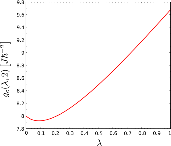
Figure 1: Critical coupling $g_{c}(\lambda,2)$ from (2.21,2.22), as a function of the pair creation/annihilation rate $\lambda$, for $d=2$ space dimensions.

Turning to the values of the critical coupling $g_{c}=g_{c}(\lambda,d)$, we consider first the $2D$ case and have

$$g(\lambda,2)=8\pi^{2}\frac{(1+\lambda)^{3}}{G(\lambda)^{2}}\,\frac{J}{\hbar^{2}}$$ (2.21)

where, using [61, eq. (2.15.20.5)], we find from (2.12)

$$G(\lambda) = \int_{0}^{\infty}\!{\rm d}u\,\int_{0}^{1}\frac{{\rm d}x\exp\left(-us_{c}\right)}{\sqrt{x(1-x)\,}}\left[\frac{1+\lambda}{2}(1+3\lambda)I_{0}(\varrho)^{2}-\frac{1-\lambda^{2}}{2}I_{1}(\varrho)^{2}+\frac{1-\lambda^{2}}{2\varrho}I_{1}(\varrho)I_{0}(\varrho)\right]$$ (2.22)

$$= \int_{0}^{1}\frac{{\rm d}x}{\sqrt{x(1-x)\,}}\left[\frac{1+3\lambda}{2}\>{}_{2}F_{1}\left(\frac{1}{2},\frac{1}{2};1;\left(1-x\frac{2\lambda}{1+\lambda}\right)^{2}\right)\right.$$

$$\left.-\frac{1-\lambda}{16}\left(1-x\frac{2\lambda}{1+\lambda}\right)^{2}\>{}_{2}F_{1}\left(\frac{3}{2},\frac{3}{2};3;\left(1-x\frac{2\lambda}{1+\lambda}\right)^{2}\right)\right.$$

$$\left.+\frac{1-\lambda}{4}\>{}_{3}F_{2}\left(\frac{1}{2},1,\frac{3}{2};2,2;\left(1-x\frac{2\lambda}{1+\lambda}\right)^{2}\right)\right]$$

This quite explicit form is more easily treated numerically than the full double integral (2.12), to be considered in generic dimensions $d$. In figure 1, we plot $g_{c}=g_{c}(\lambda,2)$ over against $\lambda$. While the two known values (2.15,2.20) for $\lambda=0$ and $\lambda=1$ are certainly reproduced, we also observe that the behaviour of $g_{c}(\lambda,2)$ is not monotonous in $\lambda$, but rather has a minimum around $\lambda\approx 0.1$. This surprising feature of a re-entrant quantum phase transition does not have an analogue in the $3D$ classical spherical model.

  

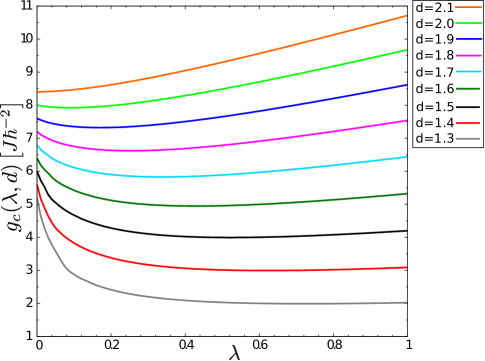
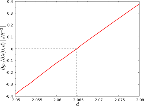
Figure 2: Left panel: Critical coupling $g_{c}(\lambda,d)$, computed from (2.23), as a function of $\lambda$ for $d=[1.3,1.4,1.5,1.6,1.7,1.8,1.9,2.0,2.1]$ from bottom to top. Right panel: slope $\left.\partial g_{c}(\lambda,d)/\partial\lambda\right|_{\lambda=0}$ of the critical coupling $g_{c}$ at $\lambda=0$, as a function of $d$. For $d\approx 2.065$, the slope vanishes.

Indeed, this re-entrant transition for $\lambda$ small enough is a generic feature of the quantum spherical model. In the left panel of figure 2, we show the critical coupling $g_{c}(\lambda,d)$, as given by

$$g_{c}(\lambda,d) = d^{3}\pi^{2}(1+\lambda)^{3}\left\{\int_{0}^{\infty}\!\!{\rm d}u\int_{0}^{1}\!{\rm d}x\>\frac{\exp(-u(1+\lambda)d/2)}{\sqrt{x(1-x)}\,}\,I_{0}(\varrho)^{d}\,\right.$$ (2.23)

$$\left.\times\left[s^{2}-d(d-1)\frac{1-\lambda^{2}}{4}\frac{I_{1}(\varrho)^{2}}{I_{0}(\varrho)^{2}}-\frac{d}{2}\frac{1-\lambda^{2}}{4}\left(1+\frac{I_{2}(\varrho)}{I_{0}(\varrho)}\right)\right]\right\}^{-2}\frac{J}{\hbar^{2}}$$

Clearly, the figure suggests that $g_{c}(\lambda,d)$ should go through a non-vanishing minimum for all dimensions $d\lesssim 2.1$.

Let us make this statement more precise. First, we observe from (2.20) that $g_{c}(1,2)>g_{c}(0,2)=8J/\hbar^{2}$. Second, from (2.19) it follows that $g_{c}(1,d)$ grows monotonously with $d$. Since $g_{c}(\lambda,2)$ is increasing with $\lambda$ for $\lambda$ large enough, see figure 1, this means that the slope of $g_{c}(\lambda,d)$ at $\lambda=1$ should be positive, viz. $\left.\partial g_{c}(\lambda,d)/\partial\lambda\right|_{\lambda=1}>0$. On the other hand, in appendix E we show that close to $\lambda=0$ one has

$$g_{c}(\lambda,d)\simeq g_{c}(0,d)-\left\{\begin{array}[]{ll}g_{(0)}\lambda^{d/2}&\mbox{\rm~{};~{}~{} if $1<d<2$}\\ g_{(1)}\lambda&\mbox{\rm~{};~{}~{} if $d>2$}\end{array}\right.$$ (2.24)

and where the known constant $g_{(0)}>0$, but the sign of the known constant $g_{(1)}$ may depend on $d$. Therefore, the slope $\left.\partial g_{c}(\lambda,d)/\partial\lambda\right|_{\lambda=0}<0$ for dimensions $1<d<2$ and diverges as $\lambda\to 0$. On the other hand, in the right panel of figure 2, we show the finite slope $\left.\partial g_{c}(\lambda,d)/\partial\lambda\right|_{\lambda=0}$ of $g_{c}$ at $\lambda=0$, for dimensions $d>2$, as a function of $d$. Clearly, the slope of $g_{c}$ at $\lambda=0$ is negative for $d\lesssim 2.065$ and becomes positive for larger values of $d$. For $d$ small enough, the slope of $g_{c}(\lambda,d)$ is negative at $\lambda=0$ and positive at $\lambda=1$. By Rolle’s theorem, the critical coupling $g_{c}(\lambda,d)$ should have a minimum at some non-vanishing value of $\lambda$, for all dimensions $d\lesssim 2.065$. This is indeed what we observe in the left panel of figure 2. In consequence, the spin-anisotropic quantum spherical model has a re-entrant quantum phase transition for dimensions $d\lesssim 2.065$.

2.4 Physical observables near quantum criticality

The scaling of the thermodynamic observables follows from the free-energy density. Since we restrict ourselves to an analysis of the zero-temperature properties of our model, the quantum coupling $g$ takes over the role of the temperature in classical spin systems, such that $t_{g}$ as defined in (2.16,2.18) takes over the role of $T-T_{c}$ in classical phase transitions. Therefore, one expects for the singular part $f^{\rm sin}$ of the free energy density

$$f=\frac{F}{{\cal{N}}}=-\frac{B^{2}}{4J}\frac{1}{\sigma}+\hbar\sqrt{\frac{gJ}{2s}}\int_{\cal{B}}\frac{{\rm d}\boldsymbol{k}}{(2\pi)^{d}}\sqrt{s-\frac{1+\lambda}{2}\sum_{j=1}^{d}\cos k_{j}\,}\>\sqrt{s-\frac{1-\lambda}{2}\sum_{j=1}^{d}\cos k_{j}\,}$$ (2.25)

to obey the following scaling behaviour

$$f^{\rm sin}(t_{g},B)=A_{1}|t_{g}|^{2-\alpha}W_{\pm}\left(A_{2}B|t_{g}|^{-\beta-\gamma}\right)$$ (2.26)

where $W_{\pm}$ are universal scaling functions, associated with the sign of $t_{g}\gtrless 0$, and $\alpha,\beta,\gamma$ are the standard critical exponents. All non-universal information on the specific model can be absorbed into the two metric factors $A_{1,2}$. Similarly, we consider the spin-spin correlation (2.6) $C(|\boldsymbol{r}|)=\langle S_{\boldsymbol{n}}S_{\boldsymbol{n}+\boldsymbol{r}}\rangle$ at zero temperature $T=0$. As shown in appendix D, we can use spatial translation- and rotation-invariance, and have for $\lambda>0$

$$C(R) = \left<S_{0}S_{R}\right>\>=\>\sqrt{\frac{\hbar^{2}g}{Js}}\int_{\cal{B}}\frac{{\rm d}\boldsymbol{k}}{(2\pi)^{d}}\sqrt{\frac{2s-(1-\lambda)\sum_{j=1}^{d}\cos k_{j}}{2s-(1+\lambda)\sum_{j=1}^{d}\cos k_{j}}\,}\,\cos k_{1}R$$ (2.27)

$$= \sqrt{\frac{\hbar^{2}g}{Js}}\frac{1}{(2\pi)^{(d+1)/2}}\frac{s-\frac{1-\lambda}{2}d}{\sqrt{\lambda(1+\lambda)d/2}\,}\>\left(\frac{1}{\xi R}\right)^{(d-1)/2}K_{\frac{d-1}{2}}\left(\frac{R}{\xi}\right)$$

where we identify the correlation length, with $s=\frac{1}{2}(1+\lambda)d+\sigma$, as follows

$$\xi=\sqrt{\frac{1+\lambda}{4}\,}\>\sigma^{-1/2}$$ (2.28)

and $K_{\nu}(x)$ is the other modified Bessel function [1]. For isotropic classical phase transitions, a long-standing result of Privman and Fisher [59] states that there exist only two independent non-universal metric factors, such as $A_{1,2}$. For quantum systems, anisotropies are possible between correlators along the spatial lattice and correlations in the (euclidean) ‘time’ direction and generated via the transfer matrix ${\cal T}=\exp\left(-\tau H\right)$. One then must distinguish ‘parallel’ distances $r_{\|}$ along the ‘time’ direction and ‘perpendicular’ distances $\boldsymbol{r}_{\perp}$ along the space direction. The correlation length $\xi=\xi_{\perp}$ considered here is spatial, whereas the ‘temporal’ correlation length $\xi_{\|}\sim(\Delta E)^{-1}$ is related to the energy gap of $H$. The anisotropy between ‘time’ and ‘space’ introduces a further metric factor which in those cases where there is a classical analogue, and therefore the dynamical exponent $z=1$, amounts simply to a further independent amplitude $D_{0}$ related to the freedom of normalisation of the quantum hamiltonian $H$. For such anisotropic or quantum systems (at $T=0$), one expects a scaling form for a two-point correlator [40, 14, 49]

$$C(R;t_{g},B)=D_{0}D_{1}R^{2-d-z-\eta}X_{\pm}\left(|\boldsymbol{R}|/\xi;D_{0}r_{\parallel}/\xi^{z};D_{2}B\left|t_{g}\right|^{-\beta-\gamma}\right)$$ (2.29)

where in the situation under study here, we have $R=|\boldsymbol{R}|=|\boldsymbol{r}_{\perp}|$ and $r_{\|}=0$. As before, $X_{\pm}$ are universal scaling functions with non-universal metric factors $D_{0,1,2}$. For isotropic systems, one has $z=1$ such that the distinction between the scaling of $\boldsymbol{r}_{\perp}$ and $r_{\|}$ is no longer necessary and $D_{0}=1$ without restriction to the generality. Then, in that situation, only two of the four metric factors $A_{1,2},D_{1,2}$ are independent, according to the long-standing Privman-Fisher hypothesis [59]. This follows by tracing the metric factors as they occur in the thermodynamic observables and using the static fluctuation-dissipation theorem. For potentially anisotropic or quantum systems, even if $z=1$, this argument has to be generalised in order to admit a potentially non-universal normalisation $D_{0}$. This leads to the following universal amplitude combinations $Q_{1,2,3}$ [40]

$$Q_{1}=A_{1}\xi_{0}^{d+z}D_{0}^{-1};\ Q_{2}=D_{2}A_{2}^{-1};\ Q_{3}=D_{0}^{\gamma/(\nu(d+z))}D_{1}A_{1}^{-1-\gamma/(\nu(d+z))}A_{2}^{-2}$$ (2.30)

where the amplitude $\xi_{0}$ is from $\xi\simeq\xi_{0}t_{g}^{-\nu}$. Here, we shall use the dependence on the parameter $\lambda>0$ to control explicitly the universality and hence to test the scaling forms (2.26,2.29).

Returning to the quantum spherical model at $T=0$, the analysis of the spherical constraint, see appendix C, has given us the dependence of the shift $t_{g}$ on the shifted spherical parameter $\sigma=s-s_{c}$. Including now the magnetic field $B$ as well, we have to leading order in $\sigma$

$$t_{g}-\sqrt{\frac{8J}{\hbar^{2}g_{c}}}\left(\frac{B}{2J}\right)^{2}\sigma^{-2}\simeq\left\{\begin{array}[]{ll}A_{<}\>\sigma^{\frac{d-1}{2}}&\mbox{\rm~{};~{}~{} if $d<3$}\\ A_{3}\ \sigma\ln\sigma&\mbox{\rm~{};~{}~{} if $d=3$}\\ A_{>}\>\sigma&\mbox{\rm~{};~{}~{} if $d>3$}\end{array}\right.$$ (2.31)

with explicitly known amplitudes $A_{<}$, $A_{3}$ and $A_{>}$. For a non-vanishing magnetic field $B\neq 0$ the magnetic contribution will always dominate the behaviour of the spherical constraint near criticality.

1. First, we treat the case $0<\lambda<1$ and $1<d<3$. From the Gibbs free energy, eq. (2.25), we find for the magnetisation near criticality

$$m(t_{g},B)=-\frac{\partial f(t_{g},B)}{\partial B}=\frac{B}{2J}\,\frac{1}{\sigma}$$ (2.32)

where the spherical constraint(2.31) must be used. The critical behaviour is extracted by moving along the quantum critical ‘isochore’ $B=0$ or else the quantum critical ‘isotherm’ $t_{g}=0$. We obtain

$$m(t_{g},0)\simeq\left[\frac{\hbar^{2}g_{c}}{8J}\right]^{1/4}\cdot{t_{g}}^{1/2}\;\;,\;\;m(0,B)\simeq A_{<}^{\frac{2}{d+3}}(2J)^{\frac{1-d}{d+3}}\left(\frac{\hbar^{2}g_{c}}{8J}\right)^{\frac{1}{d+3}}\cdot B^{\frac{d-1}{d+3}}$$ (2.33)

where we used the non-universal amplitudes from (2.31) and the value of $g_{c}=g_{c}(\lambda,d)$, which are explicitly $\lambda$-dependent.

The analogue of the susceptibility is defined by $\chi(t_{g},B)=\partial m(t_{g},B)/\partial B$. Explicitly, we find

$$\chi(t_{g},0) = \frac{A_{<}^{\frac{2}{d-1}}}{2J}\cdot t_{g}^{-\frac{2}{d-1}}$$ (2.34)

$$\chi(0,B) = \frac{d-1}{d+3}A_{<}^{\frac{2}{d+3}}(2J)^{\frac{1-d}{d+3}}\left(\frac{8J}{\hbar^{2}g_{c}}\right)^{-\frac{1}{d+3}}\cdot B^{-\frac{4}{d+3}}$$ (2.35)

In general, the specific heat is given by the second derive of the free energy with respect to the temperature (here replaced by $t_{g}$). Here, we consider its analogue, where the role of $T$ is taken over by $t_{g}$. Furthermore, in the spherical model, the spherical constraint requires a little more careful consideration, which amounts to

$$c(t_{g},B)=-\frac{\partial}{\partial t_{g}}\left(\left.\frac{\partial f^{sin}(t_{g},B)}{\partial t_{g}}\right|_{s}\right)\\$$ (2.36)

where the first derivative must be taken grand-canonically, with fixed spherical parameter, whereas the second derivative is an usual thermodynamic derivative, in the canonical ensemble, see e.g. [8, 52, 7, 35, 11, 10]. We find

$$c(t_{g},0) = c_{0}+\frac{2}{d-1}\sqrt{\frac{\hbar^{2}g_{c}}{8J}}JA_{<}^{-\frac{2}{d-1}}\cdot t_{g}^{-\frac{d-3}{d-1}}$$ (2.37)

$$c(0,B) = c_{0}+\frac{1}{d-1}\left(\frac{\hbar^{2}g_{c}}{8J}\right)^{\frac{1}{d+3}}\left(8J^{3}\right)^{\frac{d-1}{d+3}}A_{<}^{-\frac{2d}{d+3}}\cdot B^{2\frac{d-3}{d+3}}$$ (2.38)

where $c_{0}$ is an unimportant background constant.

The correlation length $\xi$, introduced in eq. (2.28), reads near criticality

$$\xi(t_{g},0) = \sqrt{\frac{1+\lambda}{4}}\,A_{<}^{\frac{1}{d-1}}\cdot t_{g}^{1/(d-1)}$$ (2.39)

$$\xi(0,B) = \sqrt{\frac{1+\lambda}{4}}\,\left(\sqrt{\frac{\hbar^{2}g_{c}}{8J}}A_{<}\right)^{\frac{1}{d+3}}(2J)^{\frac{2}{d+3}}\cdot B^{-\frac{2}{d+3}}$$ (2.40)

Here, the correlation length $\xi\sim 1/\Delta E$ is related to the lowest energy gap in the hamiltonian $H$, such that the dynamical exponent $z=1$.

Finally, for the correlation function, we have from (2.27) that at criticality, where $\sigma=0$

$$C(R)=\left\langle S_{0}S_{R}\right\rangle=\sqrt{\frac{\hbar^{2}g_{c}}{J}}\frac{\sqrt{\lambda/2}}{1+\lambda}\,\pi^{-\frac{1+d}{2}}\Gamma\left(\frac{d-1}{2}\right)R^{1-d}$$ (2.41)

In contrast to the thermodynamics observables considered before, this result holds true for arbitrary dimensions and is not restricted to $d<3$.

Table 1: Critical exponents for the quantum spherical model (1) at zero temperature, along the quantum critical isochore $B=0$, in dependence on the dimension $d$ and the coupling $\lambda$.

critical isochore		$\alpha$	$\beta$	$\gamma$	$\nu$	$\eta$	$z$
$d<3$	$\lambda\neq 0$	$(d-3)/(d-1)$	$1/2$	$2/(d-1)$	$1/(d-1)$	0	$1$
$d>3$	$\lambda\neq 0$	$0$	$1/2$	$1$	$1/2$	0	$1$
$d>0$	$\lambda=0$	$0$	$1/2$	$1$	$--$	$--$	$2$

For the interpretation of these results, we recall the conventional critical exponents and also the associated amplitudes, in the notation of [60], along the quantum critical ‘isochore’ $B=0$

$$m\simeq Dt_{g}^{\beta}\ ;\ \chi\simeq\Gamma t_{g}^{-\gamma}\ ;\ c\simeq\frac{A}{\alpha}t_{g}^{-\alpha}+c_{0}\ ;\ \xi\simeq\xi_{0}t_{g}^{-\nu}\ ;\ G(R)\sim R^{2-d-z-\eta}\ ;\ \Delta E\sim\xi^{-z}$$ (2.42)

The values of the exponents can be read off and are collected in table 1. As expected they agree with those of the classical spherical model in $d+1$ dimensions.

Along the quantum critical isotherm, $t_{g}=0$, one can define

$$c\simeq c_{0}+(A_{c}/\alpha_{c})|B|^{-\alpha_{c}}\ ;\ \chi\simeq\Gamma_{c}|B|^{-\gamma_{c}}\ ;\ B\simeq D_{c}m|m|^{\delta-1}\ ;\ \xi\simeq\xi_{c}|B|^{-\nu_{c}}$$ (2.43)

and read off the exponents, collected in table 2. The universality of this quantum phase transition is confirmed through the $\lambda$-independence of all these exponents.

Table 2: Critical exponents for the quantum spherical model (1) at zero temperature, along the quantum critical ‘isotherm’ $t_{g}=0$, in dependence on the dimension $d$ and the coupling $\lambda$.

critical isotherm		$\alpha_{c}$	$\gamma_{c}$	$\delta$	$\nu_{c}$
$d<3$	$\lambda\neq 0$	$2(d-3)/(d+3)$	$4/(d+3)$	$(d+3)/(d-1)$	$2/(d+3)$
$d>3$	$\lambda\neq 0$	$0$	$2/3$	$3$	$1/3$
$d>0$	$\lambda=0$	$0$	$-1/3$	$3$	–

In addition, the universality of full scaling scaling forms (2.26,2.29) can be tested by working out at least three universal amplitude combinations [60]. Considering the singular free energy and its derivatives, we considered three amplitude combinations which from (2.26) are expected to be universal. Explicitly

$$R_{c}=A\Gamma/D^{2} = \frac{3-d}{(d-1)^{2}}$$

$$R_{\chi}=\Gamma D_{c}B^{\delta-1} = 1$$ (2.44)

$$\delta\Gamma_{c}D_{c}^{1/\delta} = 1$$

and we give the results which follow from our explicit calculations above. The $\lambda$-independence of these three amplitude ratios is additional confirmation of the scaling form (2.26), with only two non-universal metric factors. In order to test the universality of the scaling form (2.29) of the spin-spin correlator, consider

$$Q_{1} = 2^{2-d}\frac{\Gamma\left(\frac{1-d}{2}\right)}{\Gamma\left(\frac{d-1}{2}\right)}\frac{W_{+}^{\prime\prime}(0)^{2}}{W_{+}^{\prime}(0)^{2}}X_{+}(0)$$

$$Q_{3} = 2^{\frac{2d}{d+1}}\left(\frac{\Gamma\left(\frac{d-1}{2}\right)}{\Gamma\left(\frac{1-d}{2}\right)X_{+}(0)}\right)^{\frac{2}{d+1}}\frac{W_{+}^{\prime}(0)^{\frac{1-d}{d+1}}}{W_{+}^{\prime\prime}(0)^{\frac{4}{d+1}}}$$ (2.45)

whose universality is confirmed explicitly through the $\lambda$-independence. Observe that for $1<d<3$ all universal amplitude ratios in (2.44,2.45) are finite, but that several of them they either vanish or explode when $d\to 1$ or $d\to 3$. This indicates that the scaling behaviour is going to be different (or does not even exist) when $d\geq 3$ or $d\leq 1$.

For the spin-anisotropic quantum spherical model, we can conclude that the scaling forms (2.26,2.29), and their universality, have been fully confirmed at the quantum critical point at $T=0$, $g=g_{c}(\lambda,d)$, with $1<d<3$ and $0<\lambda\leq 1$. Since the scaling functions themselves are universal, they were already calculated explicitly in the classical spherical model in $d+1$ dimensions, see e.g. [11], and need not be repeated here.

2. For $0<\lambda<1$ and $d=3$, we are working at the upper critical dimension. Therefore, we have to introduce logarithmic corrections to the scaling behaviour, see eq. (2.31). In order to work with the logarithmic terms and the magnetic field, we introduce the dimensionless field $\widehat{B}:=\sqrt{\frac{8J}{\hbar^{2}g_{c}}}\frac{B}{2J}$. In this manner, the expression $\ln\widehat{B}$ is well-defined. We find for the magnetisation

$$m(t_{g},0) \simeq \left[\frac{\hbar^{2}g_{c}}{8J}\right]^{\frac{1}{4}}\cdot{t_{g}}^{\frac{1}{2}}$$ (2.46)

$$m(0,\widehat{B}) \simeq \sqrt{\frac{\hbar^{2}g_{c}}{8J}}\left(\frac{2}{3}A_{3}\right)^{\frac{1}{3}}\cdot|\widehat{B}|^{\frac{1}{3}}|\ln|\widehat{B}||^{\frac{1}{3}}$$ (2.47)

and for the susceptibility

$$\chi(t_{g},0) \simeq \frac{A_{3}}{2J}\cdot|t_{g}|^{-1}|\ln|t_{g}||$$ (2.48)

$$\chi(0,\widehat{B}) \simeq \frac{1}{2J}\left(\frac{2A_{3}}{3}\right)^{\frac{1}{3}}\cdot|\widehat{B}|^{-\frac{2}{3}}|\ln|\widehat{B}||^{\frac{1}{3}}$$ (2.49)

In the same manner as above, we calculate the specific heat and find

$$c(t_{g},0) \simeq \sqrt{\frac{2\hbar^{2}Jg_{c}}{A_{3}^{2}}}\cdot|\ln|t_{g}||^{-1}$$ (2.50)

$$c(0,\widehat{B}) \simeq 3\sqrt{\frac{\hbar^{2}Jg_{c}}{2A_{3}^{2}}}\cdot|\ln|\widehat{B}||^{-1}\$$ (2.51)

Finally, the correlation length reads

$$\xi(t_{g},0) \simeq \sqrt{\frac{1+\lambda}{4A_{3}}}\cdot|t_{g}|^{-\frac{1}{2}}\cdot|\ln|t_{g}||^{\frac{1}{2}}$$ (2.52)

$$\xi(0,\widehat{B}) \simeq \sqrt{\frac{1+\lambda}{4}}\left(\frac{2A_{3}}{3}\right)^{\frac{1}{6}}\cdot|\widehat{B}|^{-\frac{1}{3}}|\ln|\widehat{B}||^{\frac{1}{6}}$$ (2.53)

This logarithmic behaviour can be described in terms of logarithmic sub-scaling exponents [48]

$$c \sim |t_{g}|^{-\alpha}|\ln|t_{g}||^{\widehat{\alpha}}\ ;\ m(t_{g},0)\sim|t_{g}|^{\beta}|\ln|t_{g}||^{\widehat{\beta}}\ ;\ \chi\sim|t_{g}|^{-\gamma}|\ln|t_{g}||^{\widehat{\gamma}}\ ;$$

$$\xi \sim |t_{g}|^{-\nu}|\ln|t_{g}||^{\widehat{\nu}}\ ;\ m(0,\widehat{B})\sim\widehat{B}^{1/\delta}|\ln|\widehat{B}||^{\widehat{\delta}}\ ;\ C(R)\sim R^{-(d-2+z+\eta)}|\ln R|^{\widehat{\eta}}$$ (2.54)

and we simply read off their (universal, since $\lambda$-independent) values

$$\widehat{\alpha}=-1\ ;\ \widehat{\beta}=0\ ;\ \widehat{\gamma}=1\ ;\ \widehat{\nu}=\frac{1}{2}\ ;\ \widehat{\delta}=\frac{1}{3}\ ;\ \widehat{\eta}=0$$ (2.55)

These values agree with those of the $4D$ $O(n)$-Heisenberg model in the limit $n\rightarrow\infty$ [48, 41].

3. In the case $0<\lambda<1$ and $3<d$ we expect mean-field critical behaviour. Near criticality $0<t_{g}\ll 1$, we find the observables in the same manner as in the previous parts, but with the ’linear’ spherical constraint. We find the observables along the critical $B=0$ line

$$m(t_{g},0) = \left[\frac{\hbar^{2}g_{c}}{8J}\right]^{\frac{1}{4}}\cdot{t_{g}}^{\frac{1}{2}}$$ (2.56)

$$\chi(t_{g},0) = \frac{A_{>}}{2J}\cdot t_{g}^{-1}$$ (2.57)

$$c(t_{g},0) = \frac{1}{\sqrt{2}A_{>}}\sqrt{\hbar^{2}Jg_{c}}$$ (2.58)

$$\xi(t_{g},0) = \sqrt{\frac{1+\lambda}{4}A_{>}}\cdot t_{g}^{-\frac{1}{2}}$$ (2.59)

and along the quantum critical isotherm $t_{g}=0$ they read

$$m(0,B) = \left[\frac{1}{2JA_{>}}\sqrt{\frac{\hbar^{2}g_{c}}{8J}}\right]^{\frac{1}{3}}\cdot B^{\frac{1}{3}}$$ (2.60)

$$\chi(0,B) = \frac{1}{2J}\left[\frac{A_{>}}{(2J)^{2}}\sqrt{\frac{8J}{\hbar^{2}g_{c}}}\right]^{-\frac{1}{3}}\cdot B^{-\frac{2}{3}}$$ (2.61)

$$c(0,B) = \frac{1}{\sqrt{2}A_{>}}\sqrt{\hbar^{2}Jg_{c}}$$ (2.62)

$$\xi(0,B) = \sqrt{\frac{1+\lambda}{4}}\left[\frac{(2J)^{\frac{3}{2}}\hbar\sqrt{g_{c}}}{2A_{>}}\right]^{\frac{1}{6}}\cdot B^{-\frac{1}{3}}$$ (2.63)

Reading off the critical exponents (see tables 1 and 2) yields the expected mean-field behaviour.

4. For $\lambda=0$ and $d$ arbitrary, the free energy density reads

$$f(t_{g},B)=-\frac{B^{2}}{4J}\frac{1}{\sigma}+\hbar\sqrt{\frac{gJ}{2}}\sqrt{s}$$ (2.64)

The magnetisation reads consequently

$$m(t_{g},0) \simeq \frac{1}{\sqrt{8}}\cdot{t_{g}}^{1/2}$$ (2.65)

$$m(0,B) \simeq \left(2Jd\right)^{-1/3}\cdot B^{1/3}$$ (2.66)

and the magnetic susceptibility becomes

$$\chi(t_{g},0) \simeq \frac{1}{2J}\frac{\sqrt{8}}{d}\cdot t_{g}^{-1}$$ (2.67)

$$\chi(0,B) \simeq \left(\frac{d}{2J}\right)^{1/3}\cdot B^{1/3}$$ (2.68)

The specific heat is found to be constant near criticality and along the quantum critical isotherm

$$c\simeq\frac{d^{\frac{3}{2}}}{2}J$$ (2.69)

The critical exponents are listed in tables 1 and 2. They are distinct from those of the modified quantum spherical models defined in [56, 32], where the particle number $\widehat{N}$ is conserved as well.

For the correlation function, we see a disconnected part from the zero temperature contribution. As derived in appendix D, we have to take thermal contributions into account. We then find

$$C(R)=\sqrt{\frac{\hbar^{2}g}{8Js}}+\sqrt{\frac{\hbar^{2}g}{2Js}}\exp\left(-2zs\right)I_{0}(z)^{d-1}I_{R}(z)$$ (2.70)

with $z=\sqrt{gJ\hbar^{2}/2T^{2}s}$. At criticality, we can deduce to leading order in $T$, see eq. (D.17)

$$C(R) = \sqrt{\frac{\hbar^{2}g_{c}}{4dJ}}\delta_{R,0}+\sqrt{\frac{\hbar^{2}g_{c}}{dJ}}\left(\frac{T^{2}d}{4\pi^{2}g_{c}J\hbar^{2}}\right)^{d/4}\exp\left(-\frac{R^{2}T}{2}\sqrt{\frac{d}{g_{c}J\hbar^{2}}}\right)$$ (2.71)

$$= \frac{1}{2}\frac{T}{J}\xi_{T}^{-2}\,\delta_{R,0}+\frac{T}{J}\xi_{T}^{2-d}\exp\left(-\frac{1}{2}\left(\frac{R}{\xi_{T}}\right)^{2}\right)$$

with the thermal reference length $\xi_{T}^{-4}:=T^{2}d/g_{c}J\hbar^{2}$ and where the critical coupling constant $g_{c}=g_{c}(0,d;T)$ has to be found from the spherical constraint in the non-vanishing zero-temperature limit. To leading order in $T$, this gives the condition

$$\sqrt{\frac{J}{\hbar^{2}g_{c}}}=\sqrt{\frac{1}{4d}\,}+\frac{d^{-1/2}}{(2\pi)^{d/2}}\left(\frac{d}{g_{c}J\hbar^{2}}\right)^{d/4}T^{d/2}$$ (2.72)

hence $g_{c}\simeq 4d\left(1-\frac{2/\sqrt{d}}{(4\pi)^{d/2}}\left(\frac{T}{J}\right)^{d/2}+\ldots\right)\frac{J}{\hbar^{2}}$, which illustrates how finite-temperature effects renormalise the value of $g_{c}$. The behaviour (2.71) of the correlation function does not fit into the standard phenomenology, described by the conventional critical exponents [24, 39, 62, 11].

2.5 Casimir effect in $d=1$ dimension

Although an analysis of finite-size effects is beyond the scope of this work, we add a brief comment on the Casimir effect in the $d\searrow 1$ limit, that is the case of a strip geometry, of finite width $L$, and with periodic boundary conditions.

For $1D$ quantum systems with sufficiently short-ranged interactions and a classical correspondent model such that $z=1$, conformal invariance is expected to hold at the quantum ciritcal point at temperature $T=0$, see [24, 39]. Scale-invariance alone gives for the normalised free energy density $f/D_{0}=f_{0}-L^{-2}Y(C_{1}t_{g}L^{1/\nu_{\perp}},C_{2}BL^{(\beta+\gamma/\nu_{\perp})})+{\rm o}(L^{-2})$ where $Y$ is an universal scaling function and $C_{1,2}$ and $D_{0}$ are the non-universal metric factors [59, 40]. The normalisation constant $D_{0}$ must be fixed such that the dispersion (energy-momentum) relation becomes $E(k)=|k|$ for $k\to 0$, such that energy and momenta are measured in the same units, see [39]. Then conformal invariance relates the universal value $Y(0,0)=-\pi c/6$ to the central charge of the corresponding $2D$ conformal field-theory [2]. For the quantum XY chain (1.8), $f/D_{0}$ has indeed been calculated, $Y(0,0)$ was shown to be universal and the central charge $c=\frac{1}{2}$ was found [37], as expected for a model in the universality class of the $2D$ classical Ising model [24, 39, 25].

If we want to apply the same method to the quantum spherical model in $d\searrow 1$ dimensions, we have to take into account the possibility that the critical value $s_{c}$ of the spherical parameter may acquire a finite-size correction. Explicit calculations have shown, however, that this universal finite-size amplitude vanishes, for periodic boundary conditions, when $d\searrow 1$ [54, 11]. Hence, $f/D_{0}$ can be taken over from the free fermion representation of the quantum XY chain, where the boson-fermion correspondence implies that periodic boundary condition in the even sector (to which the ground-state belongs) of the quantum spherical model corresponds to anti-periodic boundary conditions in the even sector of the fermionic model (1.9) [53]. Hence, the ground-state energy of the periodic spherical model chain is identical to the ground-state energy of the quantum XY chain, with anti-periodic boundary conditions. This is known to read [37, 39]

$$\frac{f}{D_{0}}=f_{0}(\lambda)-\frac{\pi}{6}\frac{1}{L^{2}}+\frac{\pi^{3}}{120}\left(\frac{1}{\lambda^{2}}-\frac{4}{3}\right)\frac{1}{L^{4}}+{\rm O}(L^{-6})$$ (2.73)

where $f_{0}(\lambda)$ is an explicitly known, non-universal bulk contribution to the free energy density. We see that the finite-size amplitude $Y(0,0)=-\pi/6$ is $\lambda$-independent and therefore universal, as expected [59, 40], but the higher-order finite-size corrections are non-universal. We find the value $c=1$ for the central charge in $d\searrow 1$ dimensions, as expected for a free boson.

For dimensions $d>1$, the simplifications we could use here, in the $d\searrow 1$ limit, do no longer apply such that the computation of the Casimir effect is considerably more involved, see [54, 18, 21, 11, 15, 19, 20, 14] and references therein. It would be interesting if recent attempts to formulate a conformal bootstrap for the $3D$ Ising model [26] could be brought to shed light on the interpretation of universal Casimir amplitudes.

3 Conclusions

We have explored the $T=0$ quantum critical behaviour of the spin-anisotropic quantum spherical model (1). One of our motivations was to be able to compare the effects of bosonic versus fermionic degrees of freedom, by using the information available from the quantum XY model [46, 6, 67, 36, 37, 17, 39, 47, 25]. However, the quantum spherical model has the advantage that it can be analysed exactly for arbitrary dimensions $d$, coupling $g$ and external field $B$, whereas the quantum XY model is only solved for $d=1$ and for a vanishing external field $B=0$. As to be expected, we have found a line (‘quantum critical isochore’) of quantum phase transitions and used the pair creation/annihilation rate $\lambda>0$ to test explicitly for universality along this line. The generalised Privman-Fisher scaling form, adapted to quantum criticality [59, 40, 14] allowed to test not only the universality of the exponents but also of certain universal amplitude rations and in consequence of the full scaling forms (2.25,2.27). It is known since a long time that the critical behaviour of the fermionic model along the critical isochore is universal [36, 37]; we obtained here the analogous result for the bosonic model. Merely the values of the exponents are different (in $1D$, the identified central charges also differ). In the quantum spherical model, an analogous test can also be carried out along the quantum critical isotherm $t_{g}=0$.

In the special case $\lambda=0$, the total particle number is conserved, leading to a different global symmetry and the critical behaviour is different. It is also distinct from the spherical model variants [56, 32] with a global conservation of the number of quantum particles.

In the fermionic quantum XY model, the ordered phase contains a sub-phase, for $0<g<d\sqrt{1-\lambda^{2}\,}$, with spatially oscillating correlation functions [6, 67, 36, 37, 47]. This sub-phase is characterised by level crossings in the hamiltonian energy spectrum, between the even and odd spin sectors [42], The transition line between oscillating and non-oscillating correlators, at $g=d\sqrt{1-\lambda^{2}\,}$, is characterised by the existence of certain Néel ground-states [51]. We did not succeed to detect similar properties in the bosonic quantum spherical model.

A surprising feature of the model studied here is the re-entrant quantum phase transition for dimensions $d\lesssim 2.065$ and sufficiently small values of $\lambda$. This shape of the quantum critical line could not have been anticipated from previous studies of the classical spherical model. This makes it clear that interactions between the momenta cannot always be absorbed into a change of variables.

  

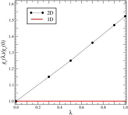
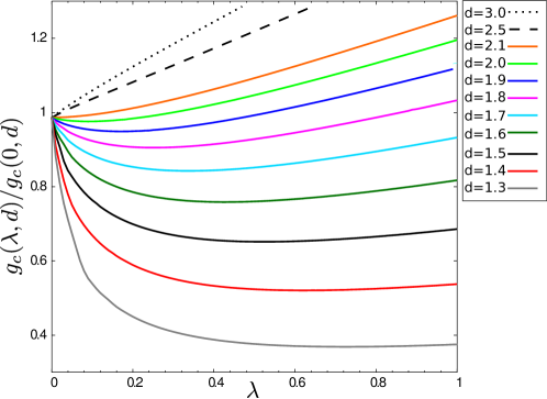
Figure 3: Left panel: normalised critical coupling $g_{c}(\lambda)/g_{c}(0)$ in the quantum XY model (1.8), as a function of the coupling $\lambda$. In $1D$, one has $g_{c}(\lambda)=1$. In $2D$, the numerically known estimates of $g_{c}(\lambda)$ [36] are given by the dots and the dashed line is a guide to the eye. Right panel: normalised critical coupling $g_{c}(\lambda,d)/g_{c}(0,d)$ in the quantum spherical model (1), as a function of $\lambda$ and for dimensions $d=[1.3,1.4,1.5,1.6,1.7,1.8,1.9,2.0,2.1,2.5,3.0]$ from bottom to top.

In figure 3, we compare the shape of the critical line $g_{c}=g_{c}(\lambda)$, normalised to the value at $g_{c}(0)$ at $\lambda=0$, of the bosonic quantum spherical model (1), with the fermionic quantum XY model. In $1D$, the latter model reduces to free fermions. Comparing the shapes of $g_{c}(\lambda,d)$, the re-entrant phase transition found in the bosonic case of the saqsm does not appear in the analogous $1D$ fermionic model, where $g_{c}(\lambda)=1$ is simply constant [6, 67]. In order to better appreciate the influence of dimensionality in the quantum XY chain on $g_{c}(\lambda)$, and in the absence of an analytic solution, the best what we can do is to compare with the few known numerical values of $g_{c}(\lambda)$ in extension of the spin hamiltonian $H_{\rm XY}$ from (1.8) to $2D$ [36]. Although those few data shown in figure 3 seem to indicate that the approach of $g_{c}(\lambda)$ towards the $\lambda=0$ case should be monotonous and hence no re-entrant transition is suggested, the available data are too few and too far apart for a final conclusion.

Since in many respects, effectively non-integer values of the dimension $d$ can also be produced by long-ranged interactions [68, 11, 32, 12, 28], one could anticipate that several of our conclusions might have qualitative analogues in long-ranged quantum phase transitions. Also, it would be interesting to see if the theory of random matrices, so sucessfully used in fermionic quantum chains [3, 44], could be brought to be applied to the kind of bosonic systems analysed here.

This illustrates that the interactions between the conjugate momenta can play a physically important role. Our results raise the question of the quantitative importance of more general kinetic terms, e.g. in O($n$)-symmetric quantum rotor models with $n$ finite. Also, one may anticipate a rich phenomenology when combining different kinds of interactions between the spins and the momenta. If such effects should be found, the spherical model would have demonstrated once more its usefulness as a heuristic device and guide towards non-trivial and interesting new types of critical behaviour.

Appendix A. Diagonalisation via a canonical transformation

The quantum hamiltonians to be diagonalised are of the form

$$H=\sum_{n,m}\left[\widehat{a}_{n}^{{\dagger}}A_{nm}\widehat{a}_{m}-\frac{1}{2}\left(\widehat{a}_{n}B_{nm}\widehat{a}_{m}+\widehat{a}_{n}^{{\dagger}}B_{nm}\widehat{a}_{m}^{{\dagger}}\right)\right]+\sum_{n}C_{n}\left(\widehat{a}_{n}+\widehat{a}_{n}^{{\dagger}}\right)$$ (A.1)

where the sums run over the ${\cal N}=N^{d}$ sites of a $d$-dimensional hyper-cubic lattice. $A$ is a hermitian matrix, $B$ a symmetric matrix and $C$ is a real, constant vector. The bosonic annihilation and creation operators $\widehat{a}_{n},\widehat{a}_{n}^{{\dagger}}$ obey the standard commutators

$${}\left[\widehat{a}_{n},\widehat{a}_{m}\right]\>=\>\left[\widehat{a}_{n}^{{\dagger}},\widehat{a}_{m}^{{\dagger}}\right]\>=\>0\;\;,\;\;\left[\widehat{a}_{n}^{{\dagger}},\widehat{a}_{m}\right]\>=\>\delta_{nm}$$ (A.2)

For $C=0$, the diagonalisation procedure follows closely the fermionic techniques of Lieb, Schultz and Mattis [53], applied to quantum Ising/XY chains. In the bosonic case, any space dimension $d$ can be treated and $C\neq 0$ is admissible. Throughout, we restrict to the case when $A$ and $B$ are real-valued (although extensions are readily formulated).

We seek a canonical transformation which brings $H$ to the form

$$H=\sum_{k}\Lambda_{k}\left(\widehat{b}_{k}^{{\dagger}}\widehat{b}_{k}+\frac{1}{2}\right)+H_{0}$$ (A.3)

where $\widehat{b}_{k},\widehat{b}_{k}^{{\dagger}}$ are again bosonic annihilation/creation operators, $\Lambda_{k}$ are the sought eigenvalues and the constant $H_{0}$ has to be determined. The required canonical transformation is of the form

$$\widehat{b}_{k}=u_{k}+\sum_{p}\left(V_{kp}\widehat{a}_{p}+W_{kp}\widehat{a}_{p}^{{\dagger}}\right)\;\;,\;\;\widehat{b}_{k}^{{\dagger}}=u_{k}+\sum_{p}\left(V_{kp}\widehat{a}_{p}^{{\dagger}}+W_{kp}\widehat{a}_{p}\right)$$ (A.4)

where the ${\cal N}\times{\cal N}$ matrices ${V}$ and ${W}$ are determined from the bosonic commutation relations and the $u_{k}$ are numbers. This gives ${V}{V}^{T}-{W}{W}^{T}={\bf 1}_{d}$ and ${V}{W}^{T}-{W}{V}^{T}={\bf 0}$, where ^T denotes the transpose and ${\bf 1}_{d}$ is the $N^{d}\times N^{d}$ unit matrix. A direct consequence of these is $({V}+{W})({V}-{W})^{T}={\bf 1}_{d}$, hence

$$({V}+{W})^{-1}=({V}-{W})^{T}\;\;,\;\;({V}-{W})^{-1}=({V}+{W})^{T}$$ (A.5)

The last conditions on $V,W$ come from the requirement that the canonical transformation (A.4) brings $H$ to its diagonal form (A.3), which means $[\widehat{b}_{k},H]=\Lambda_{k}\widehat{b}_{k}$. Hence

$$\left(V\pm W\right)\left(A\pm B\right)=\widehat{\Lambda}\left(V\mp W\right)\;\;,\;\;\left(V-W\right)C=\widehat{\Lambda}u$$ (A.6)

where $\widehat{\Lambda}={\rm diag}(\Lambda_{1},\ldots,\Lambda_{{\cal N}})$ is a diagonal matrix with the eigenvalues $\Lambda_{k}$, and the vector $u=(u_{1}\ldots,u_{{\cal N}})$. Following [53], one defines two matrices, arranged as two sets of vectors $(\boldsymbol{\Phi}_{k})_{m}:=(V+W)_{km}$ and $(\boldsymbol{\Psi}_{k})_{m}:=(V-W)_{km}$ so that by reading eq. (A.6) line by line, one has the two coupled equations

$$\boldsymbol{\Phi}_{k}^{T}\left(A+B\right)=\Lambda_{k}\boldsymbol{\Psi}_{k}^{T}\;\;,\;\;\boldsymbol{\Psi}_{k}^{T}\left(A-B\right)=\Lambda_{k}\boldsymbol{\Phi}_{k}^{T}$$ (A.7)

so that the eigenvalues $\Lambda_{k}$ can be found from the following eigenvalue equation

$$\boldsymbol{\Psi}_{k}^{T}M:=\boldsymbol{\Psi}_{k}^{T}\left(A-B\right)\left(A+B\right)=\Lambda_{k}^{2}\boldsymbol{\Psi}_{k}^{T}$$ (A.8)

Later on, we shall also need the explicit transformation of the creation/annihilation operators. For $C_{n}=0$, this reads $\widehat{b}=V\widehat{a}+W\widehat{a}^{{\dagger}}$ and its inverse becomes $\widehat{a}=V^{T}\widehat{b}-W^{T}\widehat{b}^{{\dagger}}$, along with the hermitian conjugates. We shall require this below for the calculation of correlators.

Next, we must find the eigenvalues $\Lambda_{k}$ for the specific hamiltonian (1) in the main text, with nearest-neighbour interactions. Then the diagonal form of the hamiltonian (1) is given by (A.3), where the eigenvalues $\Lambda_{\boldsymbol{k}}=s\bar{\Lambda}_{\boldsymbol{k}}$ are, for a hyper-cubic square of ${\cal N}=N^{d}$ sites in $d$ spatial dimensions and with periodic boundary conditions

$$\bar{\Lambda}_{\boldsymbol{k}}=\sqrt{1-\frac{1+\lambda}{2s}\sum_{j=1}^{d}\cos k_{j}}\>\sqrt{1-\frac{1-\lambda}{2s}\sum_{j=1}^{d}\cos k_{j}}$$ (A.9)

where the quasi-momenta $k_{j}=\frac{2\pi}{N}n_{j}$, with $n_{j}=0,1,\ldots N-1$ and $j=1,\ldots,d$ and the spherical parameter $s$.

Proof: Eq. (A.9) can be derived from the properties of cyclic matrices [4] and using mathematical induction over the dimension $d$. In what follows, we denote a cyclic ${\cal N}\times{\cal N}$ matrix, generated from a vector $(v_{1},\ldots,v_{{\cal N}})$, by

$$\mathfrak{C}\left(v_{1},\ldots,v_{\cal N}\right):=\left(\begin{array}[]{cccccc}v_{1}&v_{2}&v_{3}&\cdots&v_{{\cal N}-1}&v_{\cal N}\\ v_{\cal N}&v_{1}&v_{2}&\cdots&v_{{\cal N}-2}&v_{{\cal N}-1}\\ \vdots&&&\ddots&&\vdots\\ v_{2}&v_{3}&v_{4}&\cdots&v_{\cal N}&v_{1}\end{array}\right)$$

For the sake of this proof, we work with the reduced, dimensionless hamiltonian $H_{r}:=H/(\hbar\sqrt{g\mu})$.

Step 1: For $d=1$, ${\cal N}=N$. The matrices $A=A^{(1)}$ and $B=B^{(1)}$ are (the index refers to the value of $d$)

$$A^{(1)}=\mathfrak{C}\left(1,-\frac{1}{4s},0,\ldots,0,-\frac{1}{4s}\right)\;\;,\;\;B^{(1)}=\mathfrak{C}\left(0,\frac{\lambda}{4s},0,\ldots,0,\frac{\lambda}{4s}\right)$$

and therefore

$$M^{(1)}=\mathfrak{C}\left(1+\frac{1-\lambda^{2}}{8s^{2}},-\frac{1}{2s},\frac{1-\lambda^{2}}{16s^{2}},0,\ldots,0,\frac{1-\lambda^{2}}{16s^{2}},-\frac{1}{2s}\right)$$

is cyclic as well [4]. The eigenvalue equation (A.8) can now be solved by the ansatz $(\Psi_{k})_{n}=e^{{\rm i}kn}$. Since the cyclicity of all matrices implies periodic boundary conditions, this produces (A.9) for $d=1$ and the values of $k$ are indicated.
Step 2: In order to demonstrate the passage from $d$ to $d+1$ dimensions, consider a multi-index notation in $d+1$ dimensions

$$\boldsymbol{n}=(n_{1},n_{2},\ldots,n_{d},n_{d+1})=(\widetilde{\boldsymbol{n}}n_{d+1})\;\;,\;\;\widetilde{\boldsymbol{n}}=(n_{1},n_{2},\ldots,n_{d})$$

where individually, $n_{j}=0,1,\ldots,N-1$, with $j=1,2,\ldots,d,d+1$. In $d+1$ dimensions, the hamiltonian can be brought to a block form as follows

$$H^{(d+1)} = \sum_{\boldsymbol{n}}\left\{\left[\widehat{a}_{\boldsymbol{n}}^{{\dagger}}\widehat{a}_{\boldsymbol{n}}+\frac{1}{2}\right]-\frac{1}{4s}\sum_{j=1}^{d+1}\left[\lambda\left(\widehat{a}_{\boldsymbol{n}}\widehat{a}_{\boldsymbol{n}+\boldsymbol{e}_{j}}+\widehat{a}_{\boldsymbol{n}}^{{\dagger}}\widehat{a}_{\boldsymbol{n}+\boldsymbol{e}_{j}}^{{\dagger}}\right)+\widehat{a}_{\boldsymbol{n}}^{{\dagger}}\widehat{a}_{\boldsymbol{n}+\boldsymbol{e}_{j}}+\widehat{a}_{\boldsymbol{n}}\widehat{a}_{\boldsymbol{n}+\boldsymbol{e}_{j}}^{{\dagger}}\right]\right\}$$

$$= \sum_{\widetilde{\boldsymbol{n}}}\sum_{k=0}^{N-1}\left\{\left[\widehat{a}_{\widetilde{\boldsymbol{n}}k}^{{\dagger}}a_{\widetilde{\boldsymbol{n}}k}+\frac{1}{2}\right]\right.$$

$$\left.-\frac{1}{4s}\sum_{j=1}^{d+1}\left[\lambda\left(\widehat{a}_{\widetilde{\boldsymbol{n}}k}\widehat{a}_{\widetilde{\boldsymbol{n}}k+\widetilde{\boldsymbol{e}}_{j}k}+\widehat{a}_{\widetilde{\boldsymbol{n}}k}^{{\dagger}}\widehat{a}_{\widetilde{\boldsymbol{n}}k+\widetilde{\boldsymbol{e}}_{j}k}^{{\dagger}}\right)+\widehat{a}_{\widetilde{\boldsymbol{n}}k}^{{\dagger}}\widehat{a}_{\widetilde{\boldsymbol{n}}k+\widetilde{\boldsymbol{e}}_{j}k}+\widehat{a}_{\widetilde{\boldsymbol{n}}k}\widehat{a}_{\widetilde{\boldsymbol{n}}k+\widetilde{\boldsymbol{e}}_{j}k}^{{\dagger}}\right]\right.$$

$$\left.-\frac{1}{4s}\left[\lambda\left(\widehat{a}_{\widetilde{\boldsymbol{n}}k}\widehat{a}_{\widetilde{\boldsymbol{n}}k+1}+\widehat{a}_{\widetilde{\boldsymbol{n}}k}^{{\dagger}}\widehat{a}_{\widetilde{\boldsymbol{n}}k+1}^{{\dagger}}\right)+\widehat{a}_{\widetilde{\boldsymbol{n}}k}^{{\dagger}}\widehat{a}_{\widetilde{\boldsymbol{n}}k+1}+\widehat{a}_{\widetilde{\boldsymbol{n}}k}\widehat{a}_{\widetilde{\boldsymbol{n}}k+1}^{{\dagger}}\right]\right\}$$

$$= \sum_{k=0}^{N-1}\left\{H_{k}^{(d)}-\frac{1}{4s}\sum_{\widetilde{\boldsymbol{n}}}\left[\lambda\left(\widehat{a}_{\widetilde{\boldsymbol{n}}k}\widehat{a}_{\widetilde{\boldsymbol{n}}k+1}+\widehat{a}_{\widetilde{\boldsymbol{n}}k}^{{\dagger}}\widehat{a}_{\widetilde{\boldsymbol{n}}k+1}^{{\dagger}}\right)+\widehat{a}_{\widetilde{\boldsymbol{n}}k}^{{\dagger}}\widehat{a}_{\widetilde{\boldsymbol{n}}k+1}+\widehat{a}_{\widetilde{\boldsymbol{n}}k}\widehat{a}_{\widetilde{\boldsymbol{n}}k+1}^{{\dagger}}\right]\right\}$$

$$= \sum_{\widetilde{\boldsymbol{n}},\widetilde{\boldsymbol{m}}}\sum_{k,\ell=0}^{N-1}\left\{\widehat{a}_{\widetilde{\boldsymbol{n}}k}^{{\dagger}}A_{\widetilde{\boldsymbol{n}}k,\widetilde{\boldsymbol{m}}\ell}^{(d+1)}\widehat{a}_{\widetilde{\boldsymbol{m}}\ell}-\frac{1}{2}\left[\widehat{a}_{\widetilde{\boldsymbol{n}}k}B_{\widetilde{\boldsymbol{n}}k,\widetilde{\boldsymbol{m}}\ell}^{(d+1)}\widehat{a}_{\widetilde{\boldsymbol{m}}\ell}+\widehat{a}_{\widetilde{\boldsymbol{n}}k}^{{\dagger}}B_{\widetilde{\boldsymbol{n}}k,\widetilde{\boldsymbol{m}}\ell}^{(d+1)}\widehat{a}_{\widetilde{\boldsymbol{m}}\ell}^{{\dagger}}\right]\right\}$$

where $H_{k}^{(d)}$ is the local hamiltonian in the $k$-th $d$-dimensional layer. The interaction matrices have the block structure

$$A_{\widetilde{\boldsymbol{n}}k,\widetilde{\boldsymbol{m}}\ell}^{(d+1)} = A_{\widetilde{\boldsymbol{n}},\widetilde{\boldsymbol{m}}}^{(d)}\delta_{k,\ell}-\frac{1}{4s}\left(\delta_{\ell,k+1}+\delta_{\ell,k-1}\right){\bf 1}_{d}$$

$$B_{\widetilde{\boldsymbol{n}}k,\widetilde{\boldsymbol{m}}\ell}^{(d+1)} = B_{\widetilde{\boldsymbol{n}},\widetilde{\boldsymbol{m}}}^{(d)}\delta_{k,\ell}+\frac{\lambda}{2s}\left(\delta_{\ell,k+1}+\delta_{\ell,k-1}\right){\bf 1}_{d}$$

where ${\bf 1}_{d}$ is the $N^{d}\times N^{d}$ unit matrix. In turn, they may be written as cyclic matrices of blocks

$$A^{(d+1)}=\mathfrak{C}\left(A^{(d)},-\frac{1}{4s},0,\ldots,0,-\frac{1}{4s}\right)\;\;,\;\;B^{(d+1)}=\mathfrak{C}\left(B^{(d)},\frac{\lambda}{2s},0,\ldots,0,\frac{\lambda}{2s}\right)$$

Next, we write down the block structure of the eigenvalue equation (A.8)

$$M^{(d+1)}=\mathfrak{C}\left(M^{(d)}+\frac{1-\lambda^{2}}{8s},-\frac{A^{(d)}+\lambda B^{(d)}}{2s},\frac{1-\lambda^{2}}{16s^{2}},0,\ldots,0,\frac{1-\lambda^{2}}{16s^{2}},-\frac{A^{(d)}+\lambda B^{(d)}}{2s}\right)$$

Now, the habitual ansatz $\boldsymbol{\Psi}_{\widetilde{\boldsymbol{n}}\ell}=\boldsymbol{\Psi}_{\widetilde{\boldsymbol{n}}}\,e^{{\rm i}k\ell}$ where by induction hypothesis, $\boldsymbol{\Psi}_{\widetilde{\boldsymbol{n}}}$ is the eigenvector of the $d$-dimensional problem, gives for the eigenvalue in $d+1$ dimensions

$$\left(\bar{\Lambda}_{\widetilde{\boldsymbol{k}}k_{d+1}}^{(d+1)}\right)^{2} = \left(\bar{\Lambda}_{\widetilde{\boldsymbol{k}}}^{(d)}\right)^{2}+\frac{1-\lambda^{2}}{4s^{2}}\cos^{2}k_{d+1}-\frac{\cos k_{d+1}}{s}\left[1-\frac{1-\lambda^{2}}{2s}\sum_{j=1}^{d}\cos k_{j}\right]$$

$$= \left(\bar{\Lambda}_{\widetilde{\boldsymbol{k}}}^{(d)}\right)^{2}+\frac{1-\lambda^{2}}{4s^{2}}\cos^{2}k_{d+1}$$

$$-\frac{\cos k_{d+1}}{s}\left[\left(1-\frac{1+\lambda}{2s}\sum_{j=1}^{d}\cos k_{j}\right)\frac{1-\lambda}{2}+\left(1-\frac{1-\lambda}{2s}\sum_{j=1}^{d}\cos k_{j}\right)\frac{1+\lambda}{2}\right]$$

$$= \left(1-\frac{1+\lambda}{2s}\sum_{j=1}^{d+1}\cos k_{j}\right)\>\left(1-\frac{1-\lambda}{2s}\sum_{j=1}^{d+1}\cos k_{j}\right)$$

where in the last step the induction hypothesis (A.9) was used for $\bar{\Lambda}_{\widetilde{\boldsymbol{k}}}^{(d)}$ in $d$ dimensions. This completes the proof. q.e.d.

Finally, we find the constant $H_{0}$ in (A.3). For the sake of notational simplicity, we only treat the case $d=1$ explicitly, but we shall give the generic result at the end. Since the eigenvalues are generically two-fold degenerate, we first go over to real-valued combinations

$$\left(\bar{\boldsymbol{\Psi}}_{k}\right)_{n}:=\left\{\begin{array}[]{ll}\frac{1}{2}c_{k}\left[(\boldsymbol{\Psi}_{k})_{n}+(\boldsymbol{\Psi}_{k}^{*})_{n}\right]=c_{k}\cos nk&\mbox{\rm~{};~{}~{} if $k<N/2$}\\ \frac{1}{2{\rm i}}c_{k}\left[(\boldsymbol{\Psi}_{k})_{n}-(\boldsymbol{\Psi}_{k}^{*})_{n}\right]=c_{k}\sin nk&\mbox{\rm~{};~{}~{} if $k>N/2$}\end{array}\right.$$ (A.10)

Here, $c_{k}$ is a constant which will provide appropriate normalisation.

From (A.6), we further have $\bar{\boldsymbol{\Phi}}_{k}=\bar{\Lambda}_{k}^{-1}(A-B)\bar{\boldsymbol{\Psi}}_{k}$, hence

$$\left(\bar{\boldsymbol{\Phi}}_{k}\right)_{n}=c_{k}\bar{\Lambda}_{k}^{-1}\left(1-\frac{1+\lambda}{2s}\cos k\right)\left\{\begin{array}[]{ll}\cos nk&\mbox{\rm~{};~{}~{} if $k<N/2$}\\ \sin nk&\mbox{\rm~{};~{}~{} if $k>N/2$}\end{array}\right.$$ (A.11)

The normalisation constants follow from the bosonic commutator relations and which require

$$\sum_{n}V_{kn}^{2}-W_{kn}^{2}=\sum_{n}\left(\bar{\boldsymbol{\Phi}}_{k}\right)_{n}\left(\bar{\boldsymbol{\Psi}}_{k}\right)_{n}=1$$ (A.12)

so that finally

$$c_{k}^{2}=\frac{\bar{\Lambda}_{k}}{1-(1+\lambda)(2s)^{-1}\cos k}\left\{\begin{array}[]{ll}1/N&\mbox{\rm~{};~{}~{} if $k=0,N/2$}\\ 2/N&\mbox{\rm~{};~{}~{} else}\end{array}\right.$$ (A.13)

The extension to $d>1$ dimensions is now obvious.

While this gives the general method, we now apply it to the specific hamiltonian (1) in the main text. For a spatially constant magnetic field, all constants are equal $C_{n}=C$. From eq. (A.6), we deduce

$$u_{k}=\frac{C}{\bar{\Lambda}_{k}}\sum_{n=0}^{N-1}(\boldsymbol{\Psi}_{k})_{n}\ .$$ (A.14)

Using the geometric sum, it is obvious that $u_{k}$ vanishes for $k\neq 0$. For $k=0$, we find

$$u_{0}=CN\bar{\Lambda}_{0}^{-1}c_{0}$$ (A.15)

Thus, we are now able to write down the constant $H_{0}$ by rewriting the diagonal hamiltonian in the form $H_{r}=\frac{1}{2}\sum_{k}\bar{\Lambda}_{k}\left(\widehat{b}_{k}^{{\dagger}}\widehat{b}_{k}+\widehat{b}_{k}\widehat{b}_{k}^{{\dagger}}\right)+H_{0}$, using the transformation formula (A.4) and comparing the constant terms. We find $H_{0}=-\Lambda_{0}u_{0}^{2}$ and hence the ground-state energy reads

$$E_{0}=-\bar{\Lambda}_{0}u_{0}^{2}+\frac{1}{2}\sum_{k}\bar{\Lambda}_{k}=-\frac{C^{2}N}{1-(1+\lambda)(2s)^{-1}}+\frac{1}{2}\sum_{k}\bar{\Lambda}_{k}$$ (A.16)

with $k=\frac{2\pi}{N}n$ and $n=0,1,\ldots N-1$. The generalisation of (A.16) to $d>1$ is obvious.

Appendix B. Spherical constraint for $\lambda\neq 0,1$

We derive the spherical constraint eqs. (2.12,2.13) in the main text, for general $\lambda\neq 0,1$.

Since the magnetic field term in (2.9) is just additive, we can set $B=0$ for our purpose.

Starting from the form (2.9) of the spherical constraint, the product of the two square roots in the denominator is folded into a single factor by the Feynman identity, see e.g. [5]

$$\frac{1}{\sqrt{A\,}}\frac{1}{\sqrt{B\,}}=\frac{1}{\pi}\int_{0}^{1}\!{\rm d}x\,\frac{1}{\sqrt{x(1-x)}}\frac{1}{xA+(1-x)B}\ ,$$ (B.1)

so that the constraint becomes (with the Brillouin zone ${\cal B}=[-\pi,\pi]^{d}$)

$$\sqrt{\frac{8\pi^{2}J}{\hbar^{2}\,g}}=s^{-\frac{3}{2}}\int_{0}^{1}\frac{{\rm d}x}{\sqrt{x(1-x)}}\int_{\mathcal{B}}\frac{{\rm d}\boldsymbol{k}}{(2\pi)^{d}}\frac{s^{2}-\frac{1-\lambda^{2}}{4}\left[\sum_{j=1}^{d}\cos k_{j}\right]^{2}}{x\left(s-\frac{1+\lambda}{2}\sum_{j=1}^{d}\cos k_{j}\right)+(1-x)\left(s-\frac{1-\lambda}{2}\sum_{j=1}^{d}\cos k_{j}\right)}$$ (B.2)

However, we are looking for a representation which factorises in the momenta $k_{j}$, such that the dimension $d$ can be treated as a real parameter, in analogy to the known representations valid for $\lambda=1$. The denominator could be simply exponentiated, via the identity $G^{-1}=\int_{0}^{\infty}\!{\rm d}u\,e^{-Gu}$, but the terms in the numerator still couple the different $k_{j}$. One might consider to obtain these factors by deriving the exponential with respect to $x$ or $1-x$, but this cannot be done immediately, since the presence of $x$ in both terms in the exponential would generate unwanted contributions. It is better to introduce first an auxiliary variable

$$y=1-x$$ (B.3)

and to render it formally independent from $x$, by inserting a Delta function into an additional integration over $y$, according to

$$\int_{0}^{1}{\rm d}y\ \delta(y-1+x)f(x,y)=f(x,1-x)\;\;,\;\;\mbox{\rm for $0<x<1$.}$$ (B.4)

Now, changing the order of integrations, we can indeed re-write the denominator as an exponential and afterwards express the numerator as a derivative of this exponential. This is done by defining the differential operator

$$\mathcal{D}_{xy}:=s\left(-\frac{1}{u}\frac{\partial}{\partial x}-\frac{1}{u}\frac{\partial}{\partial y}-\frac{1}{su^{2}}\frac{\partial^{2}}{\partial x\partial y}\right)\ .$$ (B.5)

Then eq. (B.2) can be re-written as follows

$$\sqrt{\frac{8\pi^{2}J}{\hbar^{2}\,g}} = s^{-\frac{3}{2}}\int_{0}^{1}\!{\rm d}x\int_{0}^{1}\!{\rm d}y\int_{\mathcal{B}}\frac{{\rm d}\boldsymbol{k}}{(2\pi)^{d}}\int_{0}^{\infty}\!{\rm d}u\>\frac{\delta(y+x-1)}{\sqrt{xy\,}\,}\times$$ (B.6)

$$\times\mathcal{D}_{xy}\exp\left[-ux\left(s-\frac{1+\lambda}{2}\sum_{j=1}^{d}\cos k_{j}\right)-uy\left(s-\frac{1-\lambda}{2}\sum_{j=1}^{d}\cos k_{j}\right)\right]$$

$$= s^{-3/2}\int_{0}^{1}\!{\rm d}x\int_{0}^{1}\!{\rm d}y\int_{0}^{\infty}\!{\rm d}u\>\frac{\delta(y+x-1)}{\sqrt{xy\,}\,}\times$$

$$\times\mathcal{D}_{xy}\bigg{\{}\exp\left[-u(x+y)s\right]I_{0}\left(ux\frac{1+\lambda}{2}+uy\frac{1-\lambda}{2}\right)^{d}\bigg{\}}\ ,$$

since now the integrations of the $k_{j}$ factorise and can be carried out separately. Here and below, the $I_{n}(\varrho)$ denote modified Bessel functions [1].

Here, a further comment is necessary concerning the argument of the modified Bessel function. Clearly, and taking into account that $y=1-x$ will have to be put back, the argument vanishes linearly at

$$x_{0}=\frac{1}{2}\left(1-\lambda^{-1}\right)\ .$$ (B.7)

For $0<\lambda<1$, one has $x_{0}<0$ which is outside the interval of integration and need not concern us. But for $\lambda\geq 1$, one would have $0\leq x_{0}\leq\frac{1}{2}$ inside the integration interval of $x$, since the derivatives of $I_{0}$ lead to higher order modified Bessel functions $I_{n}$ with $n\geq 1$, which vanish for a vanishing argument. Then a more careful distinction of cases which takes these zeroes into account will become necessary.

We now apply the operator $\mathcal{D}_{xy}$ to the integrand in (B.6) and also define

$$\varrho:=\varrho(u,x,\lambda)=u\left(x\frac{1+\lambda}{2}+(1-x)\frac{1-\lambda}{2}\right)$$ (B.8)

Then the spherical constraint (B.6) becomes

$$\sqrt{\frac{8\pi^{2}J}{\hbar^{2}\,g}} = s^{-3/2}\int_{0}^{\infty}\!{\rm d}u\int_{0}^{1}\!{\rm d}x\>\frac{\exp\left[-us\right]}{\sqrt{x(1-x)\,}\,}\left[I_{0}(\varrho)\right]^{d}\times$$ (B.9)

$$\times\left[s^{2}-d(d-1)\frac{1-\lambda^{2}}{4}\left(\frac{I_{1}(\varrho)}{I_{0}(\varrho)}\right)^{2}-\frac{d}{2}\frac{1-\lambda^{2}}{4}\left(1+\frac{I_{2}(\varrho)}{I_{0}(\varrho)}\right)\right]\ .$$

Eqs. (B.9) and (B.8) are eqs. (2.12,2.13) in the main text.

Indeed, the dimension $d$ can now be considered as a real parameter, which offers obvious conceptual advantages. For $s\geq s_{c}=\frac{1+\lambda}{2}d$ and $\lambda\neq 0$, this integral is convergent for all $d>1$. While this representation, as it stands, holds true for all values of $\lambda$, the asymptotic analysis will become more simple for $0<\lambda<1$, where the possibility of zeroes of the $I_{n}(\varrho)$, with $n\geq 1$, need not be taken into account.

Appendix C. Asymptotic behaviour

We analyse the spherical constraint (2.12) and derive the asymptotic relations (2.18) for generic couplings $0<\lambda<1$.

1. For $1<d<3$, the leading contribution to the shift $t_{g}$ in the coupling $g$ is non-analytic. Considering the spherical constraint (2.12), non-analytic contributions come from large values of $u$ in one of the integrals. Combining eqs. (2.12,2.16), we must analyse

$$t_{g} := \sqrt{\frac{8J}{\hbar^{2}}}\left(\frac{1}{\sqrt{g}}-\frac{1}{\sqrt{g_{c}}}\right)=\frac{1}{\pi s^{3/2}}\int_{\eta}^{\infty}\!{\rm d}u\int_{0}^{1}\!{\rm d}x\>\frac{\exp\left[-us\right]}{\sqrt{x(1-x)}}\left[I_{0}(\varrho)\right]^{d}\times$$

$$\times\left[s^{2}-d(d-1)\frac{1-\lambda^{2}}{4}\left(\frac{I_{1}(\varrho)}{I_{0}(\varrho)}\right)^{2}-\frac{d}{2}\frac{1-\lambda^{2}}{4}\left(1+\frac{I_{2}(\varrho)}{I_{0}(\varrho)}\right)\right]\ .$$

for a spherical parameter $s=s_{c}+\sigma=\frac{1}{2}(1+\lambda)d+\sigma$ in the vicinity of $\sigma\to 0$. Here $\eta$ is a cut-off which helps to isolate the non-analytic contributions to $t_{g}$ and we shall let $\eta\to\infty$ at the end. Because of (2.13), the argument $\varrho$ of the modified Bessel functions never vanishes for $0<\lambda<1$. Then, in order to obtain the leading behaviour in $\sigma$, it is enough to use the leading asymptotic behaviour $I_{n}(\varrho)\simeq e^{\varrho}/\sqrt{2\pi\varrho}\left(1+{\rm O}(1/\varrho)\right)$ [1] of the modified Bessel functions. Then $I_{n}(\varrho)/I_{0}(\varrho)\simeq 1$ to leading order in $1/\varrho$ for $n=1,2$ and we arrive at

$$t_{g}\simeq\frac{1}{\pi\sqrt{s^{3}}}\int_{\eta}^{\infty}\!{\rm d}u\int_{0}^{1}\!{\rm d}x\>\frac{\exp\left[-us\right]}{\sqrt{x(1-x)}}\left(\frac{\exp\varrho}{\sqrt{2\pi\varrho}}\right)^{d}\bigg{\{}s^{2}-d(d-1)\frac{1-\lambda^{2}}{4}-d\frac{1-\lambda^{2}}{4}\bigg{\}}\ .$$ (C.2)

For convenience,we recall the definition of $\varrho$ from (2.13)

$$\varrho=\varrho(u,x,\lambda)=u\left(x\frac{1+\lambda}{2}+(1-x)\frac{1-\lambda}{2}\right)$$ (C.3)

and absorb into a single constant $\kappa$ several purely numerical factors

$$\kappa:=\left.\left(s^{2}-d^{2}\frac{1-\lambda^{2}}{4}\right)\frac{\pi^{-\frac{d}{2}-1}}{s^{3/2}}\right|_{s=s_{c}}=\sqrt{\frac{d\lambda^{2}}{2(1+\lambda)\,}}\>\frac{1}{\pi^{1+d/2}}\ .$$ (C.4)

such that the constraint becomes more compactly

$$t_{g} \simeq \kappa\int_{\eta}^{\infty}\!{\rm d}u\int_{0}^{1}\!{\rm d}x\>\frac{\exp\left[-us\right]}{\sqrt{x(1-x)}}\frac{\exp\left[ux\frac{1+\lambda}{2}d\right]\exp\left[u(1-x)\frac{1-\lambda}{2}d\right]}{u^{d/2}\left(1-\lambda(1-2x)\right)^{d/2}}$$ (C.5)

$$= \kappa\int_{\eta}^{\infty}\!{\rm d}u\int_{0}^{1}\!{\rm d}x\>\frac{\exp\left[-u\sigma\right]}{\sqrt{x(1-x)}}\frac{\exp\left[-u(1-x)d\lambda\right]}{u^{d/2}\left(1-\lambda(1-2x)\right)^{d/2}}$$

$$= 2\kappa\int_{\eta}^{\infty}\!{\rm d}u\>u^{-d/2}\exp\left[-u\sigma\right]\int_{0}^{\frac{\pi}{2}}\!{\rm d}\phi\>\frac{\exp\left[-ud\lambda\cos^{2}\phi\right]}{\left(1-\lambda\cos 2\phi\right)^{\frac{d}{2}}}$$

$$= 2\kappa\sigma^{\frac{d}{2}-1}\int_{0}^{\pi/2}\frac{{\rm d}\psi}{\left(1+\lambda\cos 2\psi\right)^{d/2}}\int_{\eta\sigma}^{\infty}\!{\rm d}v\>v^{-d/2}\exp\left[-v-vd\lambda\frac{\sin^{2}\psi}{\sigma}\right]\ .$$

where we used $s=\frac{1}{2}(1+\lambda)(x+1-x)d+\sigma$ in the 2^nd line and changed variables several times, in the 3^rd line according to $x=\sin^{2}\phi$, and in the 4^th line $v=u\sigma$ and $\phi=\frac{\pi}{2}-\psi$, and also used $\cos\phi=\sin\psi$ and $\cos 2\phi=-\cos 2\psi$.

We are interested in the asymptotic behaviour near criticality, when $0<\sigma\ll 1$. Furthermore the main contribution to the $\psi$–integral, for $v$ still finite, will come from the region where $\sin^{2}\psi/\sigma={\rm O}(1)$. But in the $\sigma\to 0^{+}$ limit we consider here $\psi$ will be small as well so that we can replace $\sin\psi\simeq\psi$. Then the main contribution to this particular integral in (C.5) should come from the region

$$\psi^{2}\lesssim\sigma\ .$$ (C.6)

Hence the leading term can be obtained by replacing the upper limit in the $\psi$-integral in (C.5) by infinity. Changing the order of integrations, we find

$$t_{g} \simeq 2\kappa\sigma^{\frac{d}{2}-1}\int_{\eta\sigma}^{\infty}\frac{{\rm d}v}{v^{d/2}}\exp\left[-v\right]\int_{0}^{\infty}\frac{{\rm d}\psi}{\left(1+\lambda\right)^{d/2}}\exp\left[-vd\lambda\frac{\psi^{2}}{\sigma}\right]$$ (C.7)

$$= \frac{2\kappa}{(1+\lambda)^{d/2}}\,\sigma^{\frac{d}{2}-1}\int_{\eta\sigma}^{\infty}\frac{{\rm d}v}{v^{d/2}}\exp\left[-v\right]\sqrt{\frac{\sigma}{vd\lambda}}\frac{\sqrt{\pi}}{2}$$

$$= \sigma^{(d-1)/2}\,\kappa\sqrt{\frac{\pi}{d\lambda}}\left(1+\lambda\right)^{-d/2}\,\Gamma\left(\frac{1-d}{2},\eta\sigma\right)\>=\>\sigma^{(d-1)/2}\,\frac{\Gamma\left(\frac{1-d}{2},\eta\sigma\right)\sqrt{\lambda/2}}{[\pi(1+\lambda)]^{(d+1)/2}}\$$

with the incomplete Gamma function $\Gamma(a,x)$ [1]. Next, we have to carry out the two limiting processes, first $\sigma\rightarrow 0^{+}$ and then $\eta\rightarrow\infty$, in exactly this order. Defining the Gamma function via analytical continuation, for $1<d<3$ we simply have $\lim_{\sigma\to 0}\Gamma(\frac{1-d}{2},\sigma)=\Gamma(\frac{1-d}{2})$ and obtain

$$t_{g}\simeq\sigma^{(d-1)/2}\,\frac{\Gamma\left(\frac{1-d}{2}\right)\sqrt{\lambda/2}}{[\pi(1+\lambda)]^{(d+1)/2}}=:A_{<}\,\sigma^{(d-1)/2}\mbox{\rm~{}~{}~{} for $1<d<3$}$$ (C.8)

2. For $d=3$, we can repeat the analysis leading to (C.7). However, the limit $\sigma\to 0^{+}$ in the incomplete Gamma function has to be taken more carefully. Using [1, eqs. (6.5.19, 5.1.11)], one has a logarithmic term

$$\Gamma(-1,x)\simeq\frac{1}{x}+C_{E}-1+\ln(x)-\frac{x}{2}+{\rm O}(x^{2})$$ (C.9)

where $C_{E}\approx 0.5772\ldots$ is Euler’s constant. Consequently, we find for the $\sigma$-dependence in $t_{g}$

$$\sigma\Gamma(-1,\eta\sigma)\simeq\frac{1}{\eta}+\left[C_{E}-1+\ln(\eta\sigma)\right]\sigma+{\rm O}(\sigma^{2})\simeq\sigma\ln\sigma$$ (C.10)

In the last expression, we merely retain the most singular term when $\sigma\to 0^{+}$ with $\eta$ finite and then dropped those terms which vanish in the $\eta\to\infty$ limit. The leading non-analytic contribution in (C.7) is

$$t_{g}\simeq\frac{\sqrt{\lambda/2}}{[\pi(1+\lambda)]^{2}}\>\sigma\ln\sigma=:A_{3}\,\sigma\ln\sigma\mbox{\rm~{};~{}~{} for $d=3$}$$ (C.11)

3. For $d>3$, the non-analytic contribution from eq. (C.7) $t_{g}\sim\sigma^{(d-1)/2}$ is of higher order than linear. The leading term in $t_{g}$ now comes from the the analytic contributions to (2.12) which was previously subtracted from the left-hand side. The leading correction term is found by a straightforward expansion in $\sigma$. We also introduce the short-hand $F(d,\lambda,\rho):=-d(d-1)\frac{1-\lambda^{2}}{4}\frac{I_{1}(\rho)^{2}}{I_{0}(\rho)^{2}}-\frac{d}{2}\frac{1-\lambda^{2}}{4}\left(1+\frac{I_{2}(\rho)}{I_{0}(\rho)}\right)$ which is obviously independent of $s$. Hence, recalling also (C.3)

$$\ \sqrt{\frac{8\pi^{2}J}{g\hbar^{2}}} = \int_{0}^{\infty}\!{\rm d}u\int_{0}^{1}\frac{{\rm d}x\ I_{0}(\varrho)^{d}}{\sqrt{x(1-x)}}\>s^{-3/2}\exp\left[-us\right]\left(s^{2}+F(d,\lambda,\varrho)\right)$$

$$\simeq \int_{0}^{\infty}\!{\rm d}u\int_{0}^{1}\frac{{\rm d}x\ I_{0}(\varrho)^{d}}{\sqrt{x(1-x)}}\left[\sqrt{s_{c}}+\frac{1}{\sqrt{s_{c}^{3}}}-\left(\frac{2us_{c}-1}{2\sqrt{s_{c}}}+\frac{3+2us_{c}}{2s_{c}^{5/2}}F(d,\lambda,\varrho)\right)\sigma\right]e^{-us_{c}}$$

In this expansion, the zeroth order gives $g_{c}$ and the first order gives the required linear contribution $t_{g}\simeq A_{>}\,\sigma$, where $A_{>}$ is given below in (C.15). Its value must be found numerically.

Summarising, we have found, for $0<\lambda\leq 1$

$$t_{g}\simeq\left\{\begin{array}[]{ll}A_{<}\>\sigma^{(d-1)/2}&\mbox{\rm~{};~{}~{} if $1<d<3$}\\ A_{3}\>\sigma\ln\sigma&\mbox{\rm~{};~{}~{} if $d=3$}\\ A_{>}\>\sigma&\mbox{\rm~{};~{}~{} if $d>3$}\end{array}\right.$$ (C.12)

with the following constant amplitudes (derived here for $0<\lambda<1$ but which can be continued to $\lambda=1$ as well)

$$A_{<} := \frac{\Gamma\left(\frac{1-d}{2}\right)\sqrt{\lambda/2}}{[\pi(1+\lambda)]^{(d+1)/2}}$$ (C.13)

$$A_{3} := \frac{\sqrt{\lambda/2}}{[\pi(1+\lambda)]^{2}}$$ (C.14)

$$A_{>} := -\frac{1}{\pi}\int_{0}^{\infty}\!{\rm d}u\int_{0}^{1}\frac{{\rm d}x\ I_{0}(\varrho)^{d}}{\sqrt{x(1-x)}}\left[\frac{2us_{c}-1}{2\sqrt{s_{c}}}+\frac{3+2us_{c}}{2s_{c}^{5/2}}\,F(d,\lambda,\varrho)\right]e^{-us_{c}}$$ (C.15)

with $s_{c}=(1+\lambda)d/2$, $F(d,\lambda,\rho)$ was defined above and (C.3) was used. On the other hand, for $\lambda>1$ the argument $\varrho$ of the $I_{n}(\varrho)$, as given by (C.3), can vanish, the analysis leading to (C.7) has to be re-done and (C.12) cannot be expected to remain valid.

Appendix D. Spin-spin correlator

Using the representation (1.5) in terms of ladder operators and then the canonical transformation (A.4,A.8) from appendix A, the spin-spin correlator is given by

$$\left<S_{\boldsymbol{n}}S_{\boldsymbol{m}}\right> = \sqrt{\frac{\hbar^{2}g}{8Js}}\left<\left(\widehat{a}_{\boldsymbol{n}}+\widehat{a}_{\boldsymbol{n}}^{\dagger}\right)\left(\widehat{a}_{\boldsymbol{m}}+\widehat{a}_{\boldsymbol{m}}^{\dagger}\right)\right>$$ (D.1)

$$= \sqrt{\frac{\hbar^{2}g}{8Js}}\sum_{\boldsymbol{k},\boldsymbol{k}^{\prime}}(\boldsymbol{\Psi}_{\boldsymbol{k}})_{\boldsymbol{n}}(\boldsymbol{\Psi}_{\boldsymbol{k}^{\prime}})_{\boldsymbol{m}}\left[\left<\widehat{b}_{\boldsymbol{k}}\widehat{b}_{\boldsymbol{k}^{\prime}}\right>+\left<\widehat{b}_{\boldsymbol{k}}^{\dagger}\widehat{b}_{\boldsymbol{k}^{\prime}}\right>+\mbox{h.c.}\right]$$ (D.2)

Since the ladder operators are bosonic, they obey Bose-Einstein-statistics. Hence

$$\left<\widehat{b}_{\boldsymbol{k}}\widehat{b}_{\boldsymbol{k}^{\prime}}\right>=\left<\widehat{b}_{\boldsymbol{k}}^{\dagger}\widehat{b}_{\boldsymbol{k}^{\prime}}^{\dagger}\right>=0\ ;\ \left<\widehat{b}_{\boldsymbol{k}}^{\dagger}\widehat{b}_{\boldsymbol{k}^{\prime}}\right>=\delta_{\boldsymbol{k},\boldsymbol{k}^{\prime}}\left(\exp\left[\Lambda_{\boldsymbol{k}}/T\right]-1\right)^{-1}$$ (D.3)

This immediately leads to

$$\left<S_{\boldsymbol{n}}S_{\boldsymbol{m}}\right>=\sqrt{\frac{\hbar^{2}g}{8Js}}\sum_{\boldsymbol{k}}(\boldsymbol{\Psi}_{\boldsymbol{k}})_{\boldsymbol{n}}(\boldsymbol{\Psi}_{\boldsymbol{k}})_{\boldsymbol{m}}\coth\left[\Lambda_{\boldsymbol{k}}/(2T)\right]$$ (D.4)

Using the real representation of the vector $\boldsymbol{\Psi}_{\boldsymbol{k}}$ from appendix A, we find for the correlator in the continuum limit, with $\boldsymbol{m}=\boldsymbol{n}+\boldsymbol{r}$

$$\left<S_{\boldsymbol{n}}S_{\boldsymbol{n}+\boldsymbol{r}}\right>=\sqrt{\frac{\hbar^{2}g}{8Js}}\int_{\cal{B}}\frac{{\rm d}\boldsymbol{k}}{(2\pi)^{d}}\sqrt{\frac{2s-(1-\lambda)\sum_{j=1}^{d}\cos k_{j}}{2s-(1+\lambda)\sum_{j=1}^{d}\cos k_{j}}}\coth\left[\Lambda_{\boldsymbol{k}}/(2T)\right]\prod_{j=1}^{d}\cos\left(r_{j}k_{j}\right)$$ (D.5)

and spatial translation-invariance is explicit, so that we can set $\boldsymbol{n}=\boldsymbol{0}$ from now on. Eq. (D.5) is an exact expression for any temperature $T$.

1. For $\lambda\neq 0$, consider the quantum phase transition at $T=0$. Then (D.5) simplifies to

$$\left<S_{\boldsymbol{0}}S_{\boldsymbol{r}}\right>=\\ \sqrt{\frac{\hbar^{2}g}{8Js}}\int_{\cal{B}}\frac{{\rm d}\boldsymbol{k}}{(2\pi)^{d}}\sqrt{\frac{2s-(1-\lambda)\sum_{j=1}^{d}\cos k_{j}}{2s-(1+\lambda)\sum_{j=1}^{d}\cos k_{j}}\,}\,\prod_{j=1}^{d}\cos\left(r_{j}k_{j}\right)$$ (D.6)

Because of explicit rotation-invariance, we can choose axes such that $\boldsymbol{r}=(R,0\ldots,0)$. Now, eq. (D.6) can be factorised by the same techniques as used in appendix B to factorise the spherical constraint. We find, with $\varrho$ from eq. (C.3)

$$\left<S_{0}S_{R}\right>=\sqrt{\frac{\hbar^{2}g}{8Js}}\frac{1}{\pi}\int_{0}^{\infty}\!{\rm d}u\int_{0}^{1}\frac{{\rm d}x\exp[-us]}{\sqrt{x(1-x)}}\left[s-\frac{1-\lambda}{2}\left((d-1)\frac{I_{1}(\varrho)}{I_{0}(\varrho)}+\frac{I_{R}^{\prime}(\varrho)}{I_{R}(\varrho)}\right)\right]I_{0}^{d-1}(\varrho)I_{R}(\varrho)$$ (D.7)

In order to work out the correlator from this representation, we now analyse the main contributions to the $u$-integral. Since the integrand vanishes for $u=0$ and $u=\infty$, it will have a maximum at some intermediate value $u_{\rm max}$ and if the integrand is sufficiently peaked around $u_{\rm max}$, this will give the main contribution. Now, the leading term of the series expansion $I_{R}(\rho)\simeq(\rho/2)^{R}/\Gamma(R+1)$, for small arguments $\rho\ll 1$, shows that for $u$ not too large, the integrand will roughly behave as $u^{R}e^{-u}$ such that $u_{\rm max}\sim R$. Since we merely interested in the large-$R$ limit, it follows that the contribution of small values of $u$ to the integral is negligible to leading order. Therefore, in order to estimate $\langle S_{0}S_{R}\rangle$, it is enough to use the $\rho\gg 1$ asymptotic form $I_{\nu}(\rho)\simeq(2\pi\rho)^{-1/2}\exp\left[\rho-\frac{\nu^{2}}{2\rho}\right]$ of the Bessel functions, such that

$$\left<S_{0}S_{R}\right>\simeq\sqrt{\frac{\hbar^{2}g}{8Js}}\frac{1}{\pi}\left(s-\frac{1-\lambda}{2}d\right)\int_{0}^{\infty}\!{\rm d}u\int_{0}^{1}{\rm d}x\,\frac{(2\pi\varrho)^{-d/2}}{\sqrt{x(1-x)}}\,\exp\left[d\varrho-us-\frac{R^{2}}{2\varrho}\right]$$ (D.8)

This can be evaluated following the lines of appendix C. We find

$$\left<S_{0}S_{R}\right>=\sqrt{\frac{\hbar^{2}g}{8Js}}\frac{(1+\lambda)^{-d/2}}{\pi^{(d+1)/2}}\frac{(s-\frac{1-\lambda}{2}d)}{\sqrt{\lambda d\,}\,}\>\sigma^{(d-1)/2}\int_{0}^{\infty}\!{\rm d}v\ v^{-(d+1)/2}\exp\left[-v-\frac{R^{2}\sigma}{(1+\lambda)}\frac{1}{v}\right]$$ (D.9)

This equation can be rewritten, using the identity $K_{\nu}(x)=\frac{1}{2}\left(\frac{x}{2}\right)^{\nu}\int_{0}^{\infty}{\rm d}vv^{-\nu-1}\exp\left[-v-x^{2}/(4v)\right]$ [33] for the modified Bessel function of the second kind, to obtain

$$\left<S_{0}S_{R}\right>=\sqrt{\frac{\hbar^{2}g}{Js}}\frac{2^{-d/2}}{\pi^{(d+1)/2}}\frac{s-\frac{1-\lambda}{2}d}{\sqrt{\lambda(1+\lambda)d}\,}\>\left(\frac{1}{\xi R}\right)^{(d-1)/2}K_{\frac{d-1}{2}}\left(\frac{R}{\xi}\right)$$ (D.10)

and where the correlation length was identified as $\xi:=\frac{1}{2}\sqrt{\frac{1+\lambda}{\sigma}}$. Very close to criticality, $\xi$ diverges, hence $R/\xi\ll 1$. At some finite distance from $g_{c}$, one has on the contrary $R/\xi\gg 1$. Now, using the leading expansions [1, eqs. (9.6.9,9.7.2)], one has the asymptotic behaviour

$$\left<S_{0}S_{R}\right>\simeq\sqrt{\frac{\hbar^{2}g}{Js}\,}\,\frac{s-\frac{1-\lambda}{2}d}{\pi^{(1+d)/2}\sqrt{\lambda(1+\lambda)d}}\times\left\{\begin{array}[]{ll}2^{-3/2}\ \Gamma\left(\frac{d-1}{2}\right)\cdot R^{1-d}&\mbox{\rm~{};~{}~{} if $R\ll\xi$}\\[2.84544pt] 2^{-d/2}\sqrt{\pi/2}\cdot\xi^{1-d}\,(\xi/R)^{d/2}\,\ e^{-R/\xi}&\mbox{\rm~{};~{}~{} if $R\gg\xi$}\end{array}\right.$$ (D.11)

with $s=s_{c}+\sigma$, $\sigma$ is related to $\xi$ and the value of $g$ has to be taken from the spherical constraint.

2. If $\lambda=0$, we have to do a more careful analysis, since the zero-temperature contribution is completely disconnected. From eq. (D.6), we see a $\delta_{R,0}$ contribution arising. Thus, the leading non-trivial contributions in this particular case are thermal and we have to re-investigate the correlation function for non-zero temperatures. Hence we return to eq. (D.5), as well as to (2.5) for the spherical constraint, in order to find the thermal corrections to the critical coupling constant $g_{c}$. Since we are still interested in a certain low-temperature limit and not in the thermal transition, we take $0<T\ll 1$ and use the asymptotic expansion $\coth x\simeq 1+2\exp(-2x)$ to obtain the leading correction. The spherical constraint in zero field then reads

$$1=\sqrt{\frac{\hbar g}{8Js}}+2\sqrt{\frac{\hbar^{2}g}{8Js}}\exp\left(-2zs\right)I_{0}\left(z\right)^{d}\left[1+\frac{d}{2s}\frac{I_{1}\left(z\right)}{I_{0}\left(z\right)}\right]$$ (D.12)

with the argument $z:=\sqrt{{gJ\hbar^{2}}/{2T^{2}s}}$. In the low-temperature limit, $z\rightarrow\infty$. From the asymptotic expansion of the modified Bessel functions, we find

$$\sqrt{\frac{8Js}{\hbar^{2}g}}\simeq 1+\frac{2{\rm e}^{-2\sigma z}}{(2\pi z)^{d/2}}\left[1+\frac{d}{2s}\left(1-\frac{1}{2z}\right)\right]$$ (D.13)

Studying this equation up to the leading order in $1/z$, at the quantum critical point $\sigma=0$, we deduce the implicit equation for the critical coupling constant $g_{c}=g_{c}(0,d;T)$

$$\sqrt{\frac{J}{\hbar^{2}g_{c}}}=\sqrt{\frac{1}{4d}}+\frac{d^{-1/2}}{(2\pi)^{d/2}}\left(\frac{d}{g_{c}J\hbar^{2}}\right)^{d/4}T^{d/2}$$ (D.14)

First of all we see, that this equation is consistent with the zero-temperature limit and reproduces $g_{c}(0,d;0)=4dJ/\hbar^{2}$ correctly. While for $d=2$, there is a simple closed solution

$$g_{c}(0,2;T)=\left(\sqrt{\frac{8J}{\hbar^{2}}}-\sqrt{\frac{2}{\pi^{2}}}\frac{T}{\sqrt{J\hbar^{2}}}\right)^{2}$$ (D.15)

eq. (D.14) cannot be solved in closed form in general.

For large distances, the same techniques as before, applied to (D.5), lead for $\lambda=0$ to

$$\langle S_{0}S_{R}\rangle=\sqrt{\frac{\hbar^{2}g}{8Js}}+\sqrt{\frac{\hbar^{2}g}{2Js}}\exp\left(-2zs\right)I_{0}(z)^{d-1}I_{R}(z)$$ (D.16)

Using the asymptotic expansion for the Bessel functions, we find at the critical point $g=g_{c}$

$$\langle S_{0}S_{R}\rangle=\sqrt{\frac{\hbar^{2}g_{c}}{4dJ}}\>\delta_{R,0}+\sqrt{\frac{\hbar^{2}g_{c}}{dJ}}\left(\frac{T^{2}d}{4\pi^{2}g_{c}J\hbar^{2}}\right)^{d/4}\exp\left(-\frac{R^{2}T}{2}\sqrt{\frac{d}{g_{c}J\hbar^{2}}}\right)$$ (D.17)

Appendix E. Critical coupling $g_{c}(\lambda,d)$ close to $\lambda=0$

In order to prove (2.24) and to understand the unexpected behaviour of the function $g_{c}(\lambda,d)$ close to $\lambda=0$, we re-investigate the equation (recall the definition (B.8) of $\varrho=\varrho(u,\lambda,d)$)

$$\sqrt{\frac{J\pi^{2}(1+\lambda)^{3}d^{3}}{\hbar^{2}g_{c}(\lambda,d)}} = \int_{0}^{\infty}\!{\rm d}u\int_{0}^{1}\!{\rm d}x\,\frac{\exp\left[-u\frac{1+\lambda}{2}d\right]}{\sqrt{x(1-x)}}\left[I_{0}(\varrho)\right]^{d}\times\left\{\left(\frac{1+\lambda}{2}d\right)^{2}\right.$$

$$\left.-d(d-1)\frac{1-\lambda^{2}}{4}\left(\frac{I_{1}(\varrho)}{I_{0}(\varrho)}\right)^{2}-\frac{d}{2}\frac{1-\lambda^{2}}{4}\left(1+\frac{I_{2}(\varrho)}{I_{0}(\varrho)}\right)\right\}$$

$$= \sqrt{\frac{J\pi^{2}d^{3}}{\hbar^{2}g_{c}(0,d)}}+G^{(1)}+G^{(2)}$$

where the two contributions $G^{(1)}$ and $G^{(2)}$ describe the leading behaviour in $\lambda$, which are non-analytic and analytic, respectively.

First, we consider the case $1<d<2$, when the leading behaviour is given by the non-analytic term $G^{(1)}$. After a change of variable $\varrho=\frac{u}{2}\left(1-\lambda+2\lambda x\right)$ in (Appendix E. Critical coupling $g_{c}(\lambda,d)$ close to $\lambda=0$), we divide the $\varrho$-integral in two parts $\int_{0}^{\infty}{\rm d}\varrho=\int_{0}^{\eta}{\rm d}\varrho+\int_{\eta}^{\infty}{\rm d}\varrho$. In the limit $\lambda\rightarrow 0^{+}$ and $\eta\rightarrow\infty$, the first integral reduces to $g_{c}(0,d)$ while the second integral will give the desired non-analytic term $G^{(1)}$, for small $\lambda$. As in appendix C, $G^{(1)}$ is analysed via the asymptotic expansions of the Bessel functions [1], which gives

$$G^{(1)} = \int_{\eta}^{\infty}\!{\rm d}\varrho\int_{0}^{1}\frac{{\rm d}x}{\sqrt{x(1-x)}}\frac{\exp\left[-2d\varrho\lambda\frac{1-x}{1-\lambda+2\lambda x}\right]}{(1-\lambda+2\lambda x)(2\pi\varrho)^{d/2}}d^{2}\lambda$$ (E.2)

$$= 2d^{2}\lambda^{d/2}\int_{0}^{\pi/2}{\rm d}\vartheta\int_{\lambda\eta}^{\infty}\!{\rm d}y\>\frac{\exp\left[-2dy\sin^{2}\vartheta\right]}{(2\pi y)^{d/2}}$$

$$= 2d^{2}\lambda^{d/2}\int_{0}^{\infty}\!{\rm d}y\>\exp\left[-dy\right]I_{0}(yd)(2\pi y)^{-d/2}$$

where in the second line, we made the substitutions $y=\lambda\varrho$ and $x=\cos^{2}\vartheta$ and in the third line recalled the identity $\sin^{2}\vartheta=\frac{1}{2}(1-\cos 2\vartheta)$ to derive $\int_{0}^{\infty}{\rm d}\vartheta\,e^{-A\sin^{2}\vartheta}=\frac{\pi}{2}\,e^{-A/2}I_{0}(A/2)$ from the defining integral representation of $I_{0}(x)$ [1]. For $1<d<2$, this is indeed the leading contribution. Explicitly, using [61, eq. (2.15.3.3)], this further simplifies to

$$\sqrt{\frac{J}{\hbar^{2}}}g_{c}(\lambda,d)^{-1/2}\simeq\frac{1}{\sqrt{4d}}+\frac{d^{(d-1)/2}}{2\pi^{(d+1)/2}}\frac{\Gamma(1-d/2)\Gamma((d-1)/2)}{\Gamma(d/2)}\>\lambda^{d/2}$$ (E.3)

with a finite, positive amplitude for all dimensions $1<d<2$.

For $d>2$, the non-analytic contribution $G^{(1)}$ in (E.3), analytically continued in $d$, is dominated by a new analytic contribution $G^{(2)}$. To obtain this, one must formally expand the integrand in (Appendix E. Critical coupling $g_{c}(\lambda,d)$ close to $\lambda=0$) to first order in $\lambda$. Of course, such as a formal expansion is only admissible up to the order where the expansion coefficient(s) converge(s). Because of the definition (B.8) of $\varrho$, in principle the Bessel functions $I_{n}(\varrho)$ should be expanded around $\lambda=0$. However, the leading term will introduce a factor $1-2x$ into the integrand and all these contributions vanish because of $\int_{0}^{1}\!{\rm d}x\,(1-2x)/\sqrt{x(1-x)}=0$. Therefore, the additional contribution reads

$$G^{(2)}=-\lambda\frac{\pi d}{2}\int_{0}^{\infty}\!{\rm d}\varrho\>\varrho\,e^{-d\varrho}I_{0}^{d}(\varrho)\left[d^{2}\left(1-\frac{I_{1}^{2}(\varrho)}{I_{0}^{2}(\varrho)}\right)+\frac{d}{2}\frac{2I_{1}^{2}(\varrho)-I_{0}^{2}(\varrho)-I_{0}(\varrho)I_{2}(\varrho)}{I_{0}^{2}(\varrho)}\right]+{\rm O}(\lambda^{2})$$ (E.4)

and the integral over $x$ has become trivial in the $\lambda\to 0$ limit. This contribution is linear in $\lambda$ and hence will dominate over $G^{(1)}$ for $d>2$. In order to study its convergence, we split as usual $\int_{0}^{\infty}\!{\rm d}\varrho=\int_{0}^{\eta}\!{\rm d}\varrho+\int_{\eta}^{\infty}\!{\rm d}\varrho$ and analyse the convergence of the second integral. Using the asymptotic expansion of the $I_{n}(\varrho)$ up to next-to-leading term in $1/\varrho$ [1], the large-$\eta$ behaviour of $G^{(2)}$ is given by $-\frac{\lambda d}{2}(2\pi)^{-d/2}\int_{\eta}^{\infty}\!{\rm d}\varrho\>\varrho^{-d/2}$ and this converges for $d>2$. For $d<2$ however, the integral $G^{(2)}$ diverges such that the formal expansion used to derive it does not exist. Then (E.3) gives indeed the leading contribution to $g_{c}(\lambda,d)$ for $\lambda\ll 1$.

This proves (2.24) in the main text.

Acknowledgements: It is a pleasure to thank J.-Y. Fortin, G. Morigi and A. Pikovsky for useful discussions. Part of this work was done during the workshop “Advances in Non-equilibrium Statistical Mechanics”. MH gratefully thanks the organisers and the Galileo Galilei Institute for Theoretical Physics for their warm and generous hospitality and the INFN for partial support. This work was also partly supported by the Collège Doctoral franco-allemand Nancy-Leipzig-Coventry (‘Systèmes complexes à l’équilibre et hors équilibre’) of UFA-DFH. SW is grateful to UFA-DFH for financial support through grant CT-42-14-II.

References

- [1] M. Abramowitz and I.A. Stegun, Handbook of Mathematical Functions, Dover (New York 1965)
-
[2]
H. Blöte, J.L. Cardy and M.P. Nightingale, Phys. Rev. Lett. 56, 742 (1984);
I. Affleck, Phys. Rev. Lett. 56, 746 (1984) - [3] A. Altland and M.R. Zirnbauer, Phys. Rev. B55, 1142 (1997).
- [4] R. Altrovandi, Special matrices of mathematical physics: stochastic, circulant, and Bell matrices, World Scientific (Singapour 2001)
- [5] D.J. Amit and V. Martín-Mayor, Field theory, the renormalization group and critical phenomena, 3rd ed., World Scientific (Singapour 1984, 32005)
- [6] E. Barouch and B.M. McCoy, Phys. Rev. A3, 786 (1971).
- [7] R.J. Baxter, Exactly solved models in statistical mechanics, Academic Press (London 1982).
- [8] T.H. Berlin and M. Kac, Phys. Rev. 86, 821 (1952).
- [9] P.F. Bienzobaz and S.R. Salinas, Physica A391, 6399 (2012) [arxiv:1203.4073].
- [10] P.F. Bienzobaz and S.R. Salinas, Rev. Bras. Ens. Fís. 35, 3311 (2013).
- [11] J.G. Brankov, D.M. Danchev and N.S. Tonchev, Theory of critical phenomena in finite-size systems, World Scientific (Singapour 2000).
- [12] M. Campa, T. Dauxois, S. Ruffo, Phys. Rep. 480, 57 (2009) [arXiv:0907.0323].
- [13] M. Campa, T. Dauxois, D. Fanelli and S. Ruffo, Physics of long-range interacting systems, Oxford University Press (Oxford 2014).
- [14] M. Campostrini, A. Pelissetto, E. Vicari, Phys. Rev. B89, 094516 (2014) [arXiv:1401.0788].
- [15] S. Caracciolo, A. Gambassi, M. Gubinelli, A. Pelissetto, Eur. Phys. J. B34, 205 (2003) [cond-mat/0304297].
- [16] M.-C. Cha and D.-G. Kim, J. Kor. Phys. Soc. 43, 165 (2003).
- [17] B.K. Chakrabarti, A. Dutta, P. Sen, Quantum Ising phases and transitions in transverse Ising model, Lecture Notes in Physics m41, Springer (Heidelberg 1996). [2nd edition by S. Suzuki, J.-I. Inoue, B. K. Chakrabarti, Lecture Notes in Physics 862, Springer (Heidelberg 2013)]
-
[18]
H. Chamati, E.S. Pisanova and N.S. Tonchev, Phys. Rev. B57, 5798 (1998);
H. Chamati, D.M. Danchev, N.S. Tonchev, Eur. Phys. J. B14, 307 (2000). - [19] H. Chamati and N.S. Tonchev, J. Phys. A39, 469 (2006) [cond-mat/0510834].
- [20] H. Chamati, J. Phys. A41, 375002 (2008) [arXiv:0805.0715].
- [21] D. Danchev and N.S. Tonchev, J. Phys. A41, 7057 (1999) [cond-mat/9806190].
- [22] E. Demler, W. Hanke, S.-C. Zhang, Rev. Mod. Phys. 76, 909 (2004) [cond-mat/0405038].
- [23] H.W. Diehl, M.A. Shpot and R.K. Zia, Phys. Rev. B68, 224415 (2003) [cond-mat/0307355].
- [24] P. di Francesco, P. Mathieu and D. Sénéchal, Conformal field-theory, Springer (Heidelberg 1997).
- [25] A. Dutta, U. Divakaran, D. Sen, B.K. Chakrabarti, T.F. Rosenbaum, G. Aeppli, [arxiv:1012.0653]
-
[26]
S. El-Showk, M. Paulos, D. Poland, S. Rychkov, D. Simmons-Duffin, A. Vichi,
Phys. Rev. D86, 025022 (2012) [arxiv:1203.6064];
S. El-Showk, M. Paulos, D. Poland, S. Rychkov, D. Simmons-Duffin, A. Vichi, J. Stat. Phys. 157, 869 (2014) [arxiv:1403.4545]. - [27] R. Fazio and H. van der Zant, Phys. Rep. 355, 235 (2001) [cond-mat/0011152]. Wiley (New York 1971).
- [28] E.J. Flores-Sola, B. Berche, R. Kenna, M. Weigel, Eur. Phys. J. B88, 28 (2015) [arXiv:1410.1377].
- [29] R. Folk and G. Moser, Phys. Rev. B47, 13992 (1993).
- [30] L. Frachebourg and M. Henkel, Physica A195, 577 (1993) [cond-mat/9212012].
- [31] P.R.S. Gomes, P.F. Bienzobaz and M. Gomes, Phys. Rev. D88, 025050 (2013) [arxiv:1305.3792].
- [32] R. Serral Gracià and Th.M. Nieuwenhuizen, Phys. Rev. E69, 056119 (2004) [cond-mat/0304150].
- [33] I. Ryzhik and I. Gradshtein, Table of Integrals, Series, and Products, Elsevier/Academic Press (Amsterdam 2007).
- [34] M.O. Hase and S.R. Salinas, J. Phys. A39, 4875 (2006) [cond-mat/0512286].
- [35] M. Henkel and C. Hoeger, Z. Phys. B55, 67 (1984).
- [36] M. Henkel, J. Phys. A17, L795 (1984); M. Henkel, J. Phys. A20, 3569 (1987).
-
[37]
M. Henkel, J. Phys. A20, 995 (1987);
T.W. Burkhardt and I. Guim, Phys. Rev. B35, 1799 (1987);
W. Hofstetter and M. Henkel, J. Phys. A29, 1359 (1996). -
[38]
M. Henkel, J. Phys. A21, L227 (1988); M. Henkel and R. Weston, J. Phys. A25, L207 (1992);
S. Allen and R.K. Pathria, J. Phys. A26, 5173 (1993);
N. Ortner and P. Wagner, SIAM Rev. 37, 428 (1995). - [39] M. Henkel, Conformal invariance and critical phenomena, Springer (Heidelberg 1999).
- [40] M. Henkel and U. Schollwöck, J. Phys. A34, 3333 (2001) [cond-mat/001006].
- [41] M. Henkel and M. Pleimling, “Non-equilibrium phase transitions vol. 2: ageing and dynamical scaling far from equilibrium”, Springer (Heidelberg 2010).
- [42] C. Hoeger, G.v. Gehlen and V. Rittenberg, J. Phys. A18, 1813 (1985).
- [43] R.M. Hornreich, M. Luban and S. Shtrikman, Phys. Rev. Lett. 35, 1678 (1975).
- [44] J. Hutchinson, J.P. Keating and F. Mezzadri, [arxiv:1503.05732].
- [45] G.S. Joyce, in C. Domb, M.S. Green (eds), Phase transitions and critical phenomena, vol. 2, Academic Press (London 1972), p. 375.
- [46] S. Katsura, Phys. Rev. 127, 1508 (1962).
- [47] D. Karevski, J. Phys. A33, L313 (2000) [cond-mat/0009038].
-
[48]
R. Kenna, D.A. Johnston and W. Janke, Phys. Rev. Lett. 96, 115701 (2006) [cond-mat/0605162];
R. Kenna, D.A. Johnston and W. Janke, Phys. Rev. Lett. 97, 155702 (2006) [cond-mat/0608127]. - [49] T.R. Kirkpatrick and D. Belitz, [arxiv:1503.04175].
- [50] J.B. Kogut, Rev. Mod. Phys. 51, 659 (1979).
- [51] J. Kurmann, H. Thomas and G. Müller, Physica 112A, 235 (1982).
- [52] H.W. Lewis and G.H. Wannier, Phys. Rev. 88, 682 (1952); erratum 90, 1131 (1953).
- [53] E. Lieb, T. Schultz and D. Mattis, Ann. of Phys. 16, 407 (1961).
- [54] J.M. Luck, Phys. Rev. B31, 3069 (1985). Elsevier/Academic Press, Amsterdam
- [55] Y.-q. Ma and W. Figueiredo, Phys. Rev. B55, 5604 (1997); Y.-q. Ma, J. Phys. Soc. Japan 68, 2361 (1999).
- [56] Th. M. Nieuwenhuizen, Phys. Rev. Lett. 74, 4293 (1995) [cond-mat/9408056].
- [57] G. Obermair, in J.I. Budnick and M.P. Kawars (eds), Dynamical Aspects of Critical Phenomena, (Gordon and Breach, New York, 1972), p. 137.
- [58] M. H. Oliveira, E.P. Raposo and M.D. Coutinho-Filho, Phys. Rev. B74, 184101 (2006).
- [59] V. Privman and M.E. Fisher, Phys. Rev. B30, 322 (1984).
- [60] V. Privman, P.C. Hohenberg and A. Aharony, in C. Domb and J.L. Lebowitz (eds), Phase transitions and critical phenomena, vol. 14, Academic Press (London 1993)
- [61] A.P. Prudnikov, Yu.A. Brychkov, O.I. Marichev, “Integrals and series vol 2: special functions”, Gordon and Breach (New York 1986).
- [62] S. Sachdev, Quantum phase transitions, Cambridge University Press (Cambridge 1999).
- [63] M. Shpot and Yu. M. Pismak, Nucl. Phys. B862, 75 (2012) [arxiv:1202.2464].
- [64] P. Shukla and S. Singh, Phys. Lett. 81A, 477 (1981); Phys. Rev. B23, 4661 (1981).
- [65] M. Srednicki, Phys. Rev. B20, 3783 (1979).
- [66] H.E. Stanley, Phys. Rev. 176, 718 (1968).
-
[67]
M. Suzuki, Prog. Theor. Phys. 46, 1337 (1971);
M. Suzuki, Prog. Theor. Phys. 56, 1454 (1976). - [68] T. Vojta, Phys. Rev. B53, 710 (1996).