Abstract

Tower of States analysis is a powerful tool for investigating phase transitions in condensed matter systems. Spontaneous symmetry breaking implies a specific structure of the energy eigenvalues and their corresponding quantum numbers on finite systems. In these lecture notes we explain the group representation theory used to derive the spectral structure for several scenarios of symmetry breaking. We give numerous examples to compute quantum numbers of the degenerate groundstates, including translational symmetry breaking or spin rotational symmetry breaking in Heisenberg antiferromagnets. These results are then compared to actual numerical data from Exact Diagonalization.

1 Introduction

Spontaneous symmetry breaking is amongst the most important and fundamental concepts in condensed matter physics. The fact that a ground- or thermal state of a system does not obey its full symmetry explains most of the well-known phase transitions in solid state physics like crystallization of a fluid, superfluidity, magnetism, superconductivity and many more. A standard concept for investigating spontaneous symmetry breaking is the notion of an order parameter. In the thermodynamic limit it is non-zero in the symmetry-broken phase and zero in the disordered phase.

Another concept to detect spontaneous symmetry breaking less widely known but equally powerful is the tower of states analysis (TOS) [1, 2]. The energy spectrum, i.e. the eigenvalues of the Hamiltonian, of a finite system has a characteristic and systematic structure in a symmetry broken phase: several eigenstates are quasi-degenerate on finite systems, become degenerate in the thermodynamic limit and possess certain quantum numbers. The TOS analysis deals with understanding the spectral structure of the Hamiltonian and predicting quantum numbers of the groundstate manifold. Also on finite systems spontaneous symmetry breaking manifests itself in the structure of the energy spectra which are accessible via numerical simulations. Most prominently, the Exact Diagonalization method [3, 4] can exactly calculate these spectra, including their quantum numbers, on moderate system sizes. Different well-established numerical techniques like the Quantum Monte Carlo technique also allow for performing energy level spectroscopy to a certain extent [5]. The predictions of TOS analysis are highly nontrivial statements which can be used to unambiguously identify symmetry broken phases. Thus TOS analysis is a powerful technique to investigate many condensed matter systems using numerical simulations. The goal of these lecture notes is to explain the specific structure of energy spectra and their quantum numbers in symmetry broken phases. The anticipated structure is then compared to several actual numerical simulations using Exact Diagonalization.

These lecture notes have been written at the kind request of the organizers of the Jülich 2016 ”Autumn School on Correlated Electrons” [6]. The notes build on and complement previously available lecture notes by Claire Lhuillier [2], by Grégoire Misguich and Philippe Sindzingre [7] and by Karlo Penc and one of the authors [8].

The outline of these notes is as follows: in Section 2 we introduce the tower of states of continuous symmetry breaking and derive its scaling behaviour. We investigate a toy model which shows most of the relevant features. Section 3 explains in detail how the multiplicities and quantum numbers in the TOS can be predicted by elementary group theoretical methods. To apply these methods we discuss several examples in Section 4 and compare them to actual numerical data from Exact Diagonalization.

2 Tower of states

We start our discussion on spontaneous symmetry breaking by investigating the Heisenberg model on the square lattice. Its Hamiltonian is given by

$$H=J\sum\limits_{\left<i,j\right>}\mathbf{S}_{i}\cdot\mathbf{S}_{j}$$ (1)

and is invariant under global SU($2$) spin rotations, i.e. a rotation of every spin on each site with the same rotational SU($2$) matrix. Therefore the total spin

$$\mathbf{S}_{\text{tot}}^{2}=\left(\sum\limits_{i}\mathbf{S}_{i}\right)^{2}=S_{\text{tot}}(S_{\text{tot}}+1)$$ (2)

is a conserved quantity of this model and every state in the spectrum of this Hamiltonian can be labeled via its total spin quantum number $S_{\text{tot}}$. The Heisenberg Hamiltonian on the square lattice has the property of being bipartite: The lattice can be divided into two sublattices $A$ and $B$ such that every term in Eq. (1) connects one site from sublattice $A$ to sublattice $B$. It was found out early [1] that the groundstate of this model bears resemblance with the classical Néel state

$$\ket{\text{N\'{e}el class.}}=\ket{\uparrow\downarrow\uparrow\downarrow\cdots}$$ (3)

where the spin-ups live on the $A$ sublattice and the spin-downs live on the $B$ sublattice. The total spin $S_{\text{tot}}$ is not a good quantum number for this state. From elementary spin algebra we know that it is rather a superposition of several states with different total spin quantum numbers. For example the 2-site state

$$\ket{\uparrow\downarrow}=\frac{\ket{\uparrow\downarrow}-\ket{\downarrow\uparrow}}{2}+\frac{\ket{\uparrow\downarrow}+\ket{\downarrow\uparrow}}{2}=\ket{S_{\text{tot}}=0,m=0}+\ket{S_{\text{tot}}=1,m=0}$$ (4)

is the superposition of a singlet ($S_{tot}=0$) and a triplet ($S_{tot}=1$). Therefore if such a state were to be a groundstate of Eq. (1) several states with different total spin would have to be degenerate. It turns out that on finite bipartite lattices this is not the case: The total groundstate of the Heisenberg model on bipartite lattices can be proven to be a singlet state with $S_{\text{tot}}=0$. This result is known as Marshall’s Theorem [9, 10, 11]. So how can the Néel state resemble the singlet groundstate? To understand this we drastically simplify the Heisenberg model and investigate a toy model whose spectrum can be fully understood analytically.

2.1 Toy model: the Lieb-Mattis model

By introducing the Fourier transformed spin operators

$$\mathbf{S}_{\mathbf{k}}=\frac{1}{\sqrt{N}}\sum\limits_{j=0}^{N}e^{i\mathbf{k}\cdot\mathbf{x}_{j}}\mathbf{S}_{j}$$ (5)

we can rewrite the original Heisenberg Hamiltonian in terms of these operators as

$$H=J\sum\limits_{\mathbf{k}\in\text{BZ}}\omega_{\mathbf{k}}\mathbf{S_{k}}\cdot\mathbf{S}_{-\mathbf{k}}$$ (6)

where $\omega_{\mathbf{k}}=\cos(k_{x})+\cos(k_{y})$ and the sum over $\mathbf{k}$ runs over the momenta within the first Brillouin zone (BZ). Let $\mathbf{k}_{0}=(\pi,\pi)$ be the ordering wavevector which is the dual to the translations that leave the square Néel state invariant. We now want to look at the truncated Hamiltonian

$$H_{\text{LM}}=2J\left(\mathbf{S}_{(0,0)}^{2}-\mathbf{S}_{\mathbf{k}_{0}}\cdot\mathbf{S}_{-\mathbf{k}_{0}}\right)$$ (7)

where we omit all Fourier components in Eq. (6) except $\mathbf{k}=(0,0)$ and $\mathbf{k}_{0}=(\pi,\pi)$. This model is called the Lieb-Mattis model [10] and has a simple analytical solution. To see this we notice that Eq. (7) can be written as

$$H_{LM}=\frac{4J}{N}\sum\limits_{i\in A,j\in B}\mathbf{S}_{i}\cdot\mathbf{S}_{j}$$ (8)

in real space, where $A$ and $B$ denote the two bipartite sublattices of the square lattice and each spin is only coupled with spins in the other sublattice. The interaction strength is equal regardless of the distance between the two spins. Thus this model is not likely to be experimentally relevant. Yet it will serve as an illustrative example how breaking the spin-rotational symmetry manifests itself in the spectrum of a finite size system. We can rewrite Eq. (8) as

$$H_{LM} =\frac{4J}{N}\left(\sum\limits_{i,j\in A\cup B}\mathbf{S}_{i}\cdot\mathbf{S}_{j}-\sum\limits_{i,j\in A}\mathbf{S}_{i}\cdot\mathbf{S}_{j}-\sum\limits_{i,j\in B}\mathbf{S}_{i}\cdot\mathbf{S}_{j}\right)$$ (9)

$$=\frac{4J}{N}(\mathbf{S}_{\text{tot}}^{2}-\mathbf{S}_{A}^{2}-\mathbf{S}_{B}^{2})$$ (10)

This shows that the Lieb-Mattis model can be considered as the coupling of two large spins $S_{A}$ and $S_{B}$ to a total spin $S_{\text{tot}}$.

We find that the operators $\mathbf{S}_{\text{tot}}^{2}$, $S_{\text{tot}}^{z}$, $\mathbf{S}_{A}^{2}$ and $\mathbf{S}_{B}^{2}$ commute with this Hamiltonian and therefore the sublattice spins $S_{A}$ and $S_{B}$ as well as the total spin $S_{\text{tot}}$ and its z-component $m_{\text{tot}}$ are good quantum numbers for this model. For a lattice with $N$ sites ($N$ even) the sublattice spins can be chosen in the range $S_{A,B}\in\{0,1,\dots,N/4\}$ and by coupling them

$$S_{\text{tot}} \in\{|S_{A}-S_{B}|,|S_{A}-S_{B}|+1,\dots,S_{A}+S_{B}\}$$ (11)

$$m_{\text{tot}} \in\{-S_{\text{tot}},-S_{\text{tot}}+1,\dots,S_{\text{tot}}\}$$ (12)

can be chosen. A state $\ket{S_{\text{tot}},m,S_{A},S_{B}}$ is thus an eigenstate of the systems with energy

$$E(S_{\text{tot}},m,S_{A},S_{B})=\frac{4J}{N}\left[S_{\text{tot}}(S_{\text{tot}}+1)-S_{A}(S_{A}+1)-S_{B}(S_{B}+1)\right]$$ (13)

independent of $m$, so each state is at least ($2S_{\text{tot}}+1$)-fold degenerate.

Tower of states

We first want to consider only the lowest energy states for each $S_{\text{tot}}$ sector. These states build the famous tower of states and collapse in the thermodynamic limit to a highly degenerate groundstate manifold, as we will see in the following.

For a given total spin $S_{\text{tot}}$ the lowest energy states are built by maximizing the last two terms in Eq. (13) with $S_{A}=S_{B}=N/4$ and

$$E_{0}(S_{\text{tot}})=E(S_{\text{tot}},m,N/4,N/4)=\frac{4J}{N}S_{\text{tot}}(S_{\text{tot}}+1)-J(\frac{N}{4}+1)$$ (14)

The groundstate of a finite system will thus be the singlet state with $S_{\text{tot}}=0$ . On a finite system the groundstate is, therefore, totally symmetric under global spin rotations and does not break the $SU(2)$-symmetry. In the thermodynamic limit $N\rightarrow\infty$, however, the energy of all these states scales to zero and all of them constitute to the groundstate manifold.

The classical Néel state with fully polarized spins on each sublattice can be built out of these states by a linear combination of all the $S_{\text{tot}}$ levels with $m_{tot}=0$ [2]. All other Néel states pointing in a different direction in spin-space can be equivalently built out of this groundstate manifold by considering linear combinations with other $m_{tot}$ quantum numbers. In the thermodynamic limit, any infinitesimal small field will force the Néel state to choose a direction and the groundstate spontaneously breaks $SU(2)$-symmetry.

The states which constitute the groundstate manifold in the thermodynamic limit can be readily identified on finite-size systems as well, where their energy and spin quantum number are given by Eq. (14). These states are called the tower of states (TOS) or also Anderson tower, thin spectrum and quasi-degenerate joint states [1, 12, 13, 14].

Excitations

The lowest excitations above the tower of states can be built by lowering the spin of one sublattice $S_{A}$ or $S_{B}$ by one, see Eq. (13). Let us set $S_{A}=N/4$ and $S_{B}=N/4-1$ which implies that $S_{\text{tot}}\in\{1,2,\dots,N/2-1\}$. We can directly compute the energy $E_{1}(S_{\text{tot}})$ of these excited states for each allowed $S_{\text{tot}}$. The energy gap to the tower of states

$$E_{\text{exc}}(S_{\text{tot}})=E_{1}(S_{\text{tot}})-E_{0}(S_{\text{tot}})=J$$ (15)

is constant. Hence, the lowest excitations of the Lieb-Mattis model are static spinflips. The next lowest excitations are spinflips on both sublattices, $S_{A}=S_{B}=N/4-1$ with excitation energy $E_{\text{exc}_{2}}=2J$ and $S_{\text{tot}}\in\{0,1,\dots,N/2-2\}$. We observe that only the energy gap of the TOS levels vanishes in the thermodynamic limit, so the TOS indeed solely contributes to the groundstate manifold.

Quantum Fluctuations

When we introduced the Lieb-Mattis model Eq. (7) from the Heisenberg model Eq. (6) we neglected all Fourier components except of $\mathbf{k}=(0,0)$ and $\mathbf{k}=\mathbf{k}_{0}$. This was a quite crude approximation and it is not guaranteed that all results for the Lieb-Mattis model will survive for the short-range Heisenberg model. To get some first results regarding this question, we can introduce small quantum fluctuations on top of the Néel groundstate of the Lieb-Mattis model and perform a perturbative spin-wave analysis in first order. This approach does not affect the scaling of the tower of states levels, but it has an important effect on the excitations. They are not static particles anymore, but become spinwaves (magnons) with a dispersion, which is linear around the ordering-wave vector $\mathbf{k}=\mathbf{k}_{0}$ and $\mathbf{k}=(0,0)$. On a finite-size lattice the momentum space is discrete with a distance proportional to $1/L$ between momentum space points, where $L$ is the linear size of the system. The energy of the lowest excitation above the TOS, the single magnon gap, therefore scales as $E_{\text{exc}}\propto J/L$ to zero. As the scaling is, however, slower for $d>1$-dimensional systems than the TOS scaling, these levels do not influence the groundstate manifold in the thermodynamic limit. Furthermore, the excitation of two magnons results in a two-particle continuum above the magnon mode.

The properties of the TOS and its excitations are summarized in Fig. 1. The left figure shows the general properties of the finite-size energy spectrum which can be expected when a continuous symmetry group is spontaneously broken in the thermodynamic limit. The right figure depicts the energy spectrum for the Heisenberg model on a square lattice with $N=32$ sites, obtained with Exact Diagonalization. One can clearly identify the TOS, the magnon dispersion and the many-particle continuum. The existence of a Néel TOS was not only confirmed numerically for the Heisenberg model on the square lattice, but also with analytical techniques beyond the simplification to the Lieb-Mattis model [1, 13, 14]. The different symbols in Fig. 1 represent different quantum numbers related to the space-group symmetries on the lattice. In the next section we will see that the structure of these quantum numbers depends on the exact shape of the symmetry-broken state and we will learn how to compute them.

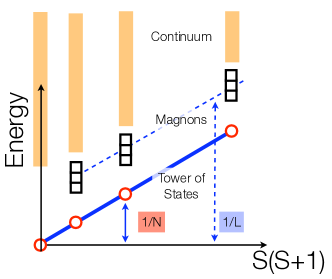
Fig. 1: (Left): Schematic finite-size energy spectrum of an antiferromagnet breaking SU($2$) spin-rotational symmetry. The TOS levels are the lowest energy levels for each total spin $S$ and scale with $1/N$ to the groundstate energy. The low energy magnon excitations are seperated from the TOS and a continuum of higher energy states and scale with $1/L$. (Right): Energy spectrum for the Heisenberg model on a square lattice from ED. The TOS levels are connected by a dashed line. The single magnon dispersion (green boxes) with $S_{\text{tot}}\in\{1,2,\dots\}$ are well separated from the TOS and the higher multi-particle continuum. The different symbols represent quantum numbers related to space-group symmetries and agree with the expectations for a Néel state (See section 3).

3 Symmetry analysis

In the analysis of excitation spectra from Exact Diagonalization on finite size simulation clusters the TOS analysis is a powerful tool to detect spontaneous symmetry breaking. As we have seen in the previous chapter explicitly for the Heisenberg antiferromagnet, symmetry breaking implies degenerate groundstates in the thermodynamic limit. On finite size simulation clusters this degeneracy is in general not an exact degeneracy. We rather expect a certain scaling of the energy differences in the thermodynamic limit. We distinguish two cases:

• Discrete symmetry breaking: In this case we have a degeneracy of finitely many states in the thermodynamic limit. The groundstate splitting $\Delta$ on finite size clusters scales as $\Delta\sim\exp(-N/\xi)$, where $N$ is the number of sites in the system.

• Continuous symmetry breaking: The groundstate in the thermodynamic limit is infinitely degenerate. The states belonging to this degenerate manifold collapse as $\Delta\sim 1/N$ on finite size clusters as we have seen in section 2. It is important to understand that these states are not the Goldstone modes of continuous symmetry breaking. Both the degenerate groundstate and the Goldstone modes appear as low energy levels on finite size clusters but have different scaling behaviours.

The scaling of these low energy states can now be investigated on finite size clusters. More importantly also their quantum numbers such as momentum, pointgroup representation or total spin can be predicted [2, 7, 15]. The detection of correct scaling behaviour together with correctly predicted quantum numbers yields very strong evidence that the system spontaneously breaks symmetry in the way that has been anticipated. This is the TOS method. In the following we will discuss how to predict the quantum numbers for discrete as well as continuous symmetry breaking. The main mathematical tool we use is the character-formula from basic group representation theory.

Lattice Hamiltonians like a Heisenberg model often have a discrete symmetry group arising from translational invariance, pointgroup invariance or some discrete local symmetry, like a spinflip symmetry. In this chapter we will first discuss the representation theory and the characters of the representations of space groups on finite lattices. We will then see how this helps us to predict the representations of the degenerate ground states in discrete as well as continuous symmetry breaking.

3.1 Representation theory for space groups

For finite discrete groups such as the space group of a finite lattice the full set of irreducible representations (irreps) can be worked out. Let us first discuss some basic groups. Let’s consider a $n\times n$ square lattice with periodic boundary conditions and a translationally invariant Hamiltonian like the Heisenberg model on it. In the following we will set the lattice spacing to $a=1$. The discrete symmetry group we consider is $\mathcal{T}=\mathbb{Z}_{n}\times\mathbb{Z}_{n}$ corresponding to the group of translations on this lattice. This is an Abelian group of order $n^{2}$. Its representations can be labeled by the momentum vectors $\mathbf{k}=(\frac{2\pi i}{n},\frac{2\pi j}{n})$, $i,j\in\{0,\cdots,n-1\}$ which just correspond to the reciprocal Bloch vectors defined on this lattice. Put differently, the vectors $\mathbf{k}$ are the reciprocal lattice points of the lattice spanned by the simulation torus of our $n\times n$ square lattice. The character $\chi_{\mathbf{k}}$ of the $\mathbf{k}$-representation is given by

$$\chi_{\mathbf{k}}(\mathbf{t})=\text{e}^{i\mathbf{k}\cdot\mathbf{t}}$$ (16)

where $\mathbf{t}\in\mathcal{T}$ is the vector of translation. This is just the usual Bloch factor for translationally invariant systems.

Let us now consider a (symmorphic) space group of the form $\mathcal{D}=\mathcal{T}\times\text{PG}$ as the discrete symmetry group of the lattice where PG is the pointgroup of the lattice. For a model on a $n\times n$ square lattice this could for example be the dihedral group of order 8, D₄, consisting of fourfold rotations together with reflections. The representation theory and the character tables of these point groups are well-established. An example for such character tables can be found in Tabs. 1 and 4 for the cyclic group $C_{4}$ and the dihedral group $D_{6}$ . Since $\mathcal{D}$ is now a product of the translation and the point group we could think that the irreducible representations of $\mathcal{D}$ are simply given by the product representations $(\mathbf{k}\otimes\rho)$ where $\mathbf{k}$ labels a momentum representation and $\rho$ an irrep of PG. But here is a small yet important caveat. We have to be careful since $\mathcal{D}$ is only a semidirect product of groups as translations and pointgroup symmetries do not necessarily commute. This alters the representation theory for this product of groups and the irreps of $\mathcal{D}$ are not just simply the products of irreps of $\mathcal{T}$ and PG. Instead the full set of irreps for this group is given by $(\mathbf{k}\otimes\rho_{\mathbf{k}})$ where $\rho_{\mathbf{k}}$ is an irrep of the so called little group $L_{\mathbf{k}}$ of $\mathbf{k}$ defined as

$$L_{\mathbf{k}}=\left\{g\in\text{PG};g(\mathbf{k})=\mathbf{k}\right\}$$ (17)

which is just the stabilizer of $\mathbf{k}$ in PG. For example, all pointgroup elements leave $\mathbf{k}=(0,0)$ invariant, thus the little group of $\mathbf{k}=(0,0)$ is the full pointgroup PG. In general, this does not hold for other momenta and only a subgroup of PG will be the little group of $\mathbf{k}$. In Fig. 4 we show the $\mathbf{k}$-points of a $6\times 6$ triangular lattice together with its little groups as an example. The $K$ point in the Brillouin zone has a D₃ little group, the $M$ point a D₂ little group. Having discussed the represenation theory for (symmorphic) space groups we state that the characters of these representations are simply given by

$$\chi_{(\mathbf{k},\rho_{\mathbf{k}})}(\mathbf{t},p)=\text{e}^{i\mathbf{k}\cdot\mathbf{t}}\chi_{\rho_{\mathbf{k}}}(p)$$ (18)

where $\mathbf{t}\in\mathcal{T}$, $p\in\text{PG}$ and $\chi_{\rho_{\mathbf{k}}}$ denotes the character of the representation $\rho_{\mathbf{k}}$ of the little group $L_{\mathbf{k}}$.

3.2 Predicting irreducible representations in spontaneous symmetry breaking

Spontaneous symmetry breaking at $T=0$ occurs when the groundstate $\ket{\psi_{\textnormal{GS}}}$ of $H$ in the thermodynamic limit is not invariant under the full symmetry group $\mathcal{G}$ of $H$. We will call a specific groundstate $\ket{\psi_{\textnormal{GS}}}$ a prototypical state and the groundstate manifold is defined by

$$V_{\textnormal{GS}}=\operatorname{span}\left\{\ket{\psi_{\textnormal{GS}}^{i}}\right\}$$ (19)

where $\ket{\psi_{\textnormal{GS}}^{i}}$ is the set of degenerate groundstates in the thermodynamic limit. This groundstate manifold space can be finite or infinite dimensional depending on the situation. For breaking a discrete finite symmetry, such as in the example given in section 4.1.2, this groundstate manifold will be finite dimensional, for breaking continuous SO($3$) spin rotational symmetry as in section 4.2 it is infinite dimensional in the thermodynamic limit. For every symmetry $g\in\mathcal{G}$ we denote by $O_{g}$ the symmetry operator acting on the Hilbert space. The groundstate manifold becomes degenerate in the thermodynamic limit and we want to calculate the quantum numbers of the groundstates in this manifold. Another way of saying this is that we want to compute the irreducible representations of $\mathcal{G}$ to which the groundstates belong to. For this we look at the action $\Gamma$ of the symmetry group $\mathcal{G}$ on $V_{\textnormal{GS}}$ defined by

$$\Gamma: \mathcal{G}\rightarrow\operatorname{Aut}(V_{\textnormal{GS}})$$ (20)

$$g\mapsto\left(\braket{\psi_{\textnormal{GS}}^{i}}{O_{g}}{\psi_{\textnormal{GS}}^{j}}\right)_{i,j}$$ (21)

This is a representation of $\mathcal{G}$ on $V_{\textnormal{GS}}$, so every group element $g\in\mathcal{G}$ is mapped to an invertible matrix on $V_{\textnormal{GS}}$. In general this representation is reducible and can be decomposed into a direct sum of irreducible representations

$$\Gamma=\bigoplus_{\rho}n_{\rho}\rho$$ (22)

These irreducible representations $\rho$ are the quantum numbers of the eigenstates in the groundstate manifold and $n_{\rho}$ are its respective multiplicities (or degeneracies). Therefore these irreps constitute the TOS for spontaneous symmetry breaking [2]. To compute the multiplicities we can use a central result from representation theory, the character formula

$$n_{\rho}=\frac{1}{|\mathcal{G}|}\sum\limits_{g\in\mathcal{G}}\overline{\chi_{\rho}(g)}\operatorname{Tr}(\Gamma(g))$$ (23)

where $\chi_{\rho}(g)$ is the character of the representation $\rho$ and $\operatorname{Tr}(\Gamma(g))$ denotes the trace over the representation matrix $\Gamma(g)$ as defined in Eq. (20). Often we have the case that

$$\braket{\psi_{\textnormal{GS}}}{O_{g}}{\psi_{\textnormal{GS}}^{\prime}}=\begin{cases}1\text{ if }O_{g}\ket{\psi_{\textnormal{GS}}^{\prime}}=\ket{\psi_{\textnormal{GS}}}\\ 0\text{ otherwise}\end{cases}$$ (24)

With this we can simplify Eq. (23) to what we call the character-stabilizer formula

$$n_{\rho}=\frac{1}{|\text{Stab}(\ket{\psi_{\textnormal{GS}}})|}\sum\limits_{g\in\text{Stab}(\ket{\psi_{\textnormal{GS}}})}\chi_{\rho}(g)$$ (25)

where

$$\text{Stab}(\ket{\psi_{\textnormal{GS}}})\equiv\{g\in\mathcal{G}:\;O_{g}\ket{\psi_{\textnormal{GS}}}=\ket{\psi_{\textnormal{GS}}}\}$$ (26)

is the stabilizer of a prototypical state $\ket{\psi_{\textnormal{GS}}}$  . We see that for applying the character-stabilizer formula in Eq. (25) only two ingredients are needed:

• the stabilizer $\text{Stab}(\ket{\psi_{\textnormal{GS}}})$ of a prototypical state $\ket{\psi_{\textnormal{GS}}}$ in the groundstate manifold

• the characters of the irreducible representations of the symmetry group $\mathcal{G}$

We want to remark that in the case of $\mathcal{G}=\mathcal{D}\times\mathcal{C}$ where $\mathcal{D}$ is a discrete symmetry group such as the spacegroup of a lattice and $\mathcal{C}$ is a continuous symmetry group such as SO($3$) rotations for Heisenberg spins the Eqs. (23) and (25) include integrals over Lie groups additionally to the sum over the elements of the discrete symmetry group $\mathcal{D}$. Furthermore also the characters for Lie groups like SO($3$) are well-known. For an element $R\in$ SO($3$) the irreducible representations are labeled by the spin $S$ and its characters are given by

$$\chi_{S}(R)=\frac{\sin\left[(S+\frac{1}{2})\phi\right]}{\sin\frac{\phi}{2}}$$ (27)

where $\phi\in[0,2\pi]$ is the angle of rotation of the spin rotation $R$. We work out several examples for this case in section 4.2 and compare the results to actual numerical data from Exact Diagonalization.

4 Examples

4.1 Discrete symmetry breaking

In this section we want to apply the formalism of section 3 to systems, where only a discrete symmetry group is spontaneously broken but not a continuous one. In this case, the ground-state of the system in the thermodynamic limit is described by a superposition of a finite number of degenerate eigenstates with different quantum numbers. On finite-size systems, however, the symmetry cannot be broken spontaneously and a unique groundstate will be found. The other states constituting to the degenerate eigenspace in the thermodynamic limit exhibit a finite-size energy gap which is exponentially small in the system size $N$, $\Delta\propto\mbox{e}^{-N/\xi}$. The quantum numbers of these quasi-degenerate set of eigenstates are defined by the symmetry-broken state in the thermodynamic limit.

4.1.1 Introduction to valence-bond solids

In section 2 we have seen that the classically ordered Néel state is a candidate to describe the groundstate of the antiferromagnetic Heisenberg model Eq. (1) with $J>0$ in the thermodynamic limit on a bipartite lattice. The energy expectation value of this state on a single bond is $e_{\text{N\'{e}el}}=-J/4$.

The state which minimizes the energy of a single bond is, however, a singlet state $\ket{S=0}$ formed by the two spins on the bond with energy $e_{\text{VB}}=-3J/4$, called a valence bond (VB) or dimer. A valence bond covering of an $N$-site lattice can then be described by a tensor product of $N/2$ VBs, where each site belongs to exactly one VB. Another possible candidate for the thermodynamic groundstate of Eq. (1) is then a superposition of all possible VB coverings with only nearest neighbour VBs. Such states do not break the $SU(2)$ spin-rotational symmetry as $S_{\text{tot}}=0$ and are in general not eigenstates of the Hamiltonian: Acting with the operator $\mathbf{S}_{i}\cdot\mathbf{S}_{j}$ between sites $i$ and $j$ belonging to two different VBs changes the VB configuration.

This manifold of VB coverings is highly degenerate. As the VB coverings are in general not eigenstates of the Hamiltonian, they encounter quantum fluctuations. The energy corrections due to these fluctuations are typically not equivalent for different coverings, although the bare energies are identical. The VB coverings with the largest energy gain are selected by the fluctuations as the true groundstate configurations. If this order-by-disorder mechanism [19, 20] selects regular patterns of VB coverings, the discrete lattice symmetries can be spontaneously broken in the thermodynamic limit, and a valence bond solid (VBS) can be formed. Fig. 2 and Fig. 3 show two different VBS states on the square lattice. VBSs show no long-range spin order, but long-range dimer-correlations $\langle(\mathbf{S}_{a}\cdot\mathbf{S}_{a^{\prime}})(\mathbf{S}_{b}\cdot\mathbf{S}_{b^{\prime}})\rangle$ where $a,a^{\prime}$ and $b,b^{\prime}$ label sites on individual dimers. In section 4.1.2 we will see how different VBS states can be identified and distinguished by the quantum numbers of the quasi-degenerate groundstate manifold on finite-size systems.

The groundstate of the Heisenberg model Eq. (1) on the square lattice is not a VBS but a Néel state, which has a lower variational energy already on the classical level. Nevertheless, several models featuring VBS groundstates are known in 1- and 2-D [21, 22, 23, 24, 25]. Interestingly, in [26] a model was proposed, which shows a direct continuous quantum phase transition between a Néel state and a VBS. This transition exhibits very exotic, non-classical behaviour and is called deconfined quantum critical point [27].

4.1.2 Identification of VBSs from finite-size spectra

Columnar valence-bond solid

A columnar VBS (cVBS) on a square lattice is shown in Fig. 2. Four equivalent states can be found, indicating that there will be a four-fold quasi-degenerate groundstate manifold. A cVBS breaks the translational and point-group symmetries of an isotropic SU(2)-invariant Hamiltonian on the lattice spontaneously but not the continuous spin symmetry group since it is a singlet and thus invariant under spin rotations.

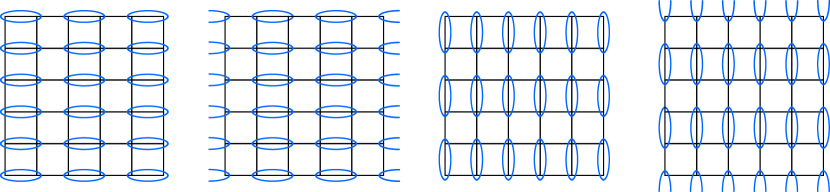
Fig. 2: The four columnar VBS coverings of a square lattice. Valence bonds (spin singlets) are indicated by blue ellipses.

In the following we use Eq. (25) to compute the symmetry sectors of the groundstate manifold. The discrete symmetry group we consider is

$$\mathcal{G}=\mathcal{D}=\mathcal{T}\times\text{PG}$$ (28)

where $\mathcal{T}=\mathbb{Z}_{2}\times\mathbb{Z}_{2}=\{1,t_{x},t_{y},t_{x}t_{y}\}$ are the non-trivial lattice translations with translation vectors

$$\mathbf{t}_{1}=(0,0),\quad\mathbf{t}_{x}=(1,0),\quad\mathbf{t}_{y}=(0,1),\quad\mathbf{t}_{xy}=(1,1)$$ (29)

and $\text{PG}=\text{C}_{4}$ denotes the point-group of four-fold lattice rotations. To compute the groundstate symmetry sectors we do not need to consider the full symmetry group $\mathcal{G}$ but only the stabilizer $\text{Stab}(\ket{\Psi_{cVBS}})$, leaving one of the states in Fig. 2 unchanged. Without loss of generality we choose the first covering as prototype $\ket{\Psi_{cVBS}}$. The stabilizer is given by

$$\text{Stab}(\ket{\Psi_{cVBS}})=\{1\times 1\}\cup\{1\times C_{2}\}\cup\{t_{y}\times 1\}\cup\{t_{y}\times C_{2}\}$$ (30)

where $C_{2}$ denotes the rotation about an angle $\pi$ around the center of a plaquette.

The irreducible representations (irreps) of the group of lattice translations $\mathcal{T}$ can be labelled by the allowed momenta $\mathbf{k}$

$$\mathbf{k}\in\mbox{Irreps}(\mathcal{T})=\{(0,0),(\pi,0),(0,\pi),(\pi,\pi)\},$$ (31)

and the corresponding characters for an element $t\in\mathcal{T}$ are

$$\chi_{\mathbf{k}}(t)=\mathrm{e}^{i\mathbf{k}\cdot\mathbf{t}}.$$ (32)

The irreps (called A, B and E, see [16]) and characters for the point-group $\text{C}_{4}$ are tabulated in Tab. 1.

$\text{C}_{4}$	$1$	$C_{4}$	$C_{2}$	$(C_{4})^{3}$
A	+1	+1	+1	+1
B	+1	-1	+1	-1
Ea	+1	+i	-1	-i
Eb	+1	-i	-1	+i

Table 1: Character table for pointgroup $\mathbf{C}_{4}$.

Using the character-stabilizer formula Eq. (25) we can now reduce the representation induced by the state $\ket{\Psi_{cVBS}}$ to irreducible representations to get the quantum numbers of the quasi-degenerate groundstate manifold. Let us explicitely consider $\mathbf{k}=(0,0)$ as an example:

$$n_{(0,0)A} =n_{(0,0)B}=\frac{1}{|\text{Stab}(\ket{\Psi_{cVBS}})|}\sum_{d\in\text{Stab}(\ket{\Psi_{cVBS}})}\chi_{A}(d)\chi_{\mathbf{k}=(0,0)}(d)$$ (33)

$$=\frac{1}{4}\left[1\cdot e^{i\mathbf{k}\cdot(0,0)}+1\cdot e^{i\mathbf{k}\cdot(0,0)}+1\cdot e^{i\mathbf{k}\cdot(0,1)}+1\cdot e^{i\mathbf{k}\cdot(0,1)}\right]=1$$ (34)

$$n_{(0,0)E_{a}} =n_{(0,0)E_{b}}=\frac{1}{|\text{Stab}(\ket{\Psi_{cVBS}})|}\sum_{d\in\text{Stab}(\ket{\Psi_{cVBS}})}\chi_{B}(d)\chi_{\mathbf{k}=(0,0)}(d)$$ (35)

$$=\frac{1}{4}\left[1\cdot e^{i\mathbf{k}\cdot(0,0)}+(-1)\cdot e^{i\mathbf{k}\cdot(0,0)}+1\cdot e^{i\mathbf{k}\cdot(0,1)}+(-1)\cdot e^{i\mathbf{k}\cdot(0,1)}\right]=0$$ (36)

Eventually, the cVBS covering will be described by a four-fold quasi-degenerate groundstate manifold with the following quantum numbers.

$$\chi(\ket{\Psi_{cVBS}})=(0,0)\mbox{A}\oplus(0,0)\mbox{B}\oplus(\pi,0)\mbox{A}\oplus(0,\pi)\mbox{A}.$$ (37)

VBS states are a superposition of spin singlets on the lattice, therefore the spin quantum number for all levels in the groundstate manifold must be trivial, $S_{\text{tot}}=0$.

Staggered valence-bond solid

The columnar VBS is not the only regular dimer covering of the square lattice. Another possible regular covering is the staggered VBS (sVBS), where again four equivalent configurations span the groundstate manifold. One of these configurations is shown in Fig. 3.

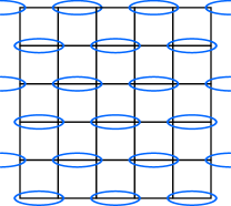
Fig. 3: One of the four identical staggered VBS coverings on the square lattice.

Similarly, also the sVBS spontaneously breaks the translational and point-group symmetries of an isotropic Hamiltonian, but not the spin-rotational symmetry. Following the same steps as before we can compute the quantum numbers of the four quasi-degenerate groundstates for the sVBS. The stabilizer turns out to be different to the case of the cVBS and thus also the decomposition into irreps yields a different result:

$$\chi(\ket{\Psi_{sVBS}})=(0,0)\mbox{A}\oplus(0,0)\mbox{B}\oplus(\pi,\pi)\mbox{E}_{a}\oplus(\pi,\pi)\mbox{E}_{b}.$$ (38)

Tab. 2 shows a comparison of the irreducible representations in the groundstate manifold of the cVBS and sVBS states.

Irreps	cVBS	sVBS
$(0,0)$ A	1	1
$(0,0)$ B	1	1
$(\pi,0)$ A	1	0
$(0,\pi)$ A	1	0
$(\pi,\pi)\text{E}_{a}$	0	1
$(\pi,\pi)\text{E}_{b}$	0	1

Table 2: Multiplicities of the irreducible representations in the four-fold degenerate groundstate manifolds of the columnar and staggered VBS on a square lattice.

By a careful analysis of the quasi-degenerate states and their quantum numbers on finite systems it is thus possible to identify and distinguish different VBS phases which spontaneously break the space group symmetries in the thermodynamic limit.

4.2 Continuous symmetry breaking

In this section we give several examples of systems breaking continuous SO($3$) symmetry. We discuss the introductory example of the square lattice Heisenberg antiferromagnet, calculate the irreps in the TOS and compare this to actual energy spectra from Exact Diagonalization on a finite lattice in section 4.2.1. In section 4.2.2 we discuss three magnetic orders on the triangular lattice and an extended Heisenberg model where all of these are stabilized. We present results from Exact Diagonalization and compare the representations in these spectra to the predictions from TOS analysis. Finally, we introduce quadrupolar order and show that also this kind of symmetry breaking can be analyzed using the TOS technique in section 4.2.3.

4.2.1 Heisenberg antiferromagnet on the square lattice

We now give a first example how the TOS method can be applied to predict the structure of the tower of states for magnetically ordered phases. We look at the Néel state of the antiferromagnet on the bipartite square lattice with sublattices $A$ and $B$. A prototypical state in the groundstate manifold is given by

$$\ket{\psi}=\ket{\uparrow\downarrow\uparrow\downarrow\cdots}$$ (39)

where all spins point up on sublattice $A$ and down on sublattice $B$. The symmetry group $\mathcal{G}=\mathcal{D}\times\mathcal{C}$ of the model we consider is a product between discrete translational symmetry $\mathcal{D}=\mathbb{Z}_{2}\times\mathbb{Z}_{2}=\left\{1,t_{x},t_{y},t_{xy}\right\}$ and spin rotational symmetry $\mathcal{C}=\text{SO(3)}$. We remark that we restrict our translational symmetry group to $\mathcal{D}=\mathbb{Z}_{2}\times\mathbb{Z}_{2}$ instead of $\mathcal{D^{\prime}}=\mathbb{Z}\times\mathbb{Z}$ because the Néel state transforms trivially under two-site translations $(t_{x})^{2},(t_{y})^{2}$. Thus, only the representations of $\mathcal{D^{\prime}}$ trivial under two-site translations are relevant; these are exactly the representations of $\mathcal{D}$. Put differently we only have to consider the translations in the unitcell of the magnetic structure which in the present case can be chosen as a $2$-by-$2$ cell. Furthermore, we will for now neglect pointgroup symmetries like rotations and reflections of the lattice to simplify calculations. At the end of this section we give results where also these symmetry elements are incorporated.

The groundstate manifold $V_{\text{GS}}$ we consider are the states related to $\ket{\psi}$ by an element of the symmetry group $\mathcal{G}$, i.e.

$$V_{\text{GS}}=\left\{O_{g}\ket{\psi};g\in\mathcal{G}\right\}$$ (40)

The symmetry elements in $\mathcal{G}$ that leave our prototypical state $\ket{\psi}$ invariant are given by two sets of elements:

• No translation in real space or a diagonal $t_{xy}$ translation together with a spin rotation $R_{z}(\alpha)$ around the $z$-axis with an arbitrary angle $\alpha$.

• Translation by one site, $t_{x}$ or $t_{y}$, followed by a rotation $R_{a}(\pi)$ of $180^{\circ}$ around an axis $a\perp z$ perpendicular to the $z$-axis.

So the stabilizer of our prototype state $\ket{\psi}$ is given by

$$\text{Stab}(\ket{\psi})=\left\{1\times R_{z}(\alpha)\right\}\cup\left\{t_{xy}\times R_{z}(\alpha)\right\}\cup\left\{t_{x}\times R_{a}(\pi)\right\}\cup\left\{t_{y}\times R_{a}(\pi)\right\}$$ (41)

The representations of the discrete symmetry group can be labeled by four momenta $\mathbf{k}\in\left\{(0,0),\;(0,\pi),\;(\pi,0),\;(\pi,\pi)\right\}$ with corresponding characters

$$\chi_{\mathbf{k}}(t)=\text{e}^{i\mathbf{k}\cdot\mathbf{t}}$$

where $\mathbf{t}$ denotes the translation vector corresponding to $t$. The continuous symmetry group we consider is the Lie group SO($3$). Its representations are labeled by the total spin $S$. The character of the spin-$S$ representation is given by

$$\chi_{S}(R)=\frac{\sin\left[(S+\frac{1}{2})\phi\right]}{\sin\frac{\phi}{2}}$$

where $\phi\in[0,2\pi]$ is the angle of rotation of the element $R\in\text{SO(}3\text{)}$. We see that spin rotations with different axes but same rotational angle give rise to the same character. The representations of the total symmetry group $\mathcal{G}=\mathcal{D}\times\mathcal{C}$ are now just the product representations of $\mathcal{D}$ and $\mathcal{C}$. Therefore also the characters of representations of $\mathcal{G}$ are the product of characters of $\mathcal{D}$ and $\mathcal{C}$. We label these representations by $(\mathbf{k},S)$ where $\mathbf{k}$ denotes the lattice momentum and $S$ the total spin. To derive the multiplicities of the representations $(\mathbf{k},S)$ in the groundstate manifold, we now apply the character-stabilizer formula, Eq. (25). In the case of the square antiferromagnet this yields

$$n_{(\mathbf{k},S)}\,=\quad e^{i\mathbf{k}\cdot 0}\frac{1}{4\left|R_{z}(\alpha)\right|}\int\limits_{0}^{2\pi}d\alpha\chi_{S}(R_{z}(\alpha))+e^{i\mathbf{k}\cdot(\mathbf{e}_{x}+\mathbf{e}_{y})}\frac{1}{4\left|R_{z}(\alpha)\right|}\int\limits_{0}^{2\pi}d\alpha\chi_{S}(R_{z}(\alpha))$$ (42)

$$+e^{i\mathbf{k}\cdot\mathbf{e}_{x}}\frac{1}{4\left|R_{a}(\pi)\right|}\int\limits_{0}^{2\pi}da\chi_{S}(R_{a}(\pi))+e^{i\mathbf{k}\cdot\mathbf{e}_{y}}\frac{1}{4\left|R_{a}(\pi)\right|}\int\limits_{0}^{2\pi}da\chi_{S}(R_{a}(\pi))$$ (43)

We compute

$$\left|R_{z}(\alpha)\right|=\left|R_{a}(\pi)\right|=\int\limits_{0}^{2\pi}d\phi=2\pi$$

$$\frac{1}{2\pi}\int\limits_{0}^{2\pi}d\alpha\chi_{S}(R_{z}(\alpha))=\frac{1}{2\pi}\int\limits_{0}^{2\pi}d\alpha\frac{\sin\left[(S+\frac{1}{2})\alpha\right]}{\sin\frac{\alpha}{2}}=\frac{1}{2\pi}\int\limits_{0}^{2\pi}d\alpha\sum\limits_{l=-S}^{S}e^{il\alpha}=1$$ (44)

and

$$\frac{1}{2\pi}\int\limits_{0}^{2\pi}da\chi_{S}(R_{a}(\pi))=\frac{1}{2\pi}\int\limits_{0}^{2\pi}da\frac{\sin\left[(S+\frac{1}{2})\pi\right]}{\sin\frac{\pi}{2}}=(-1)^{S}$$ (45)

Putting this together gives the final result for the multiplicities of the representations in the tower of states

$$n_{\left((0,0),S\right)} =\frac{1}{4}\left(1\cdot 1+1\cdot 1+1\cdot(-1)^{S}+1\cdot(-1)^{S}\right)=\left\{\begin{array}[]{l}1\text{ if }S\text{ even}\\ 0\text{ if }S\text{ odd}\end{array}\right.$$ (48)

$$n_{\left((\pi,\pi),S\right)} =\frac{1}{4}\left(1\cdot 1+1\cdot 1-1\cdot(-1)^{S}-1\cdot(-1)^{S}\right)=\left\{\begin{array}[]{l}0\text{ if }S\text{ even}\\ 1\text{ if }S\text{ odd}\end{array}\right.$$ (51)

$$n_{\left((0,\pi),S\right)} =\frac{1}{4}\left(1\cdot 1-1\cdot 1+1\cdot(-1)^{S}-1\cdot(-1)^{S}\right)=0$$ (52)

$$n_{\left((\pi,0),S\right)} =\frac{1}{4}\left(1\cdot 1-1\cdot 1-1\cdot(-1)^{S}+1\cdot(-1)^{S}\right)=0$$ (53)

Tab. 3 lists the computed multiplicities of the irreducible representations where additionally the $\text{D}_{4}$ point group was considered in the symmetry analysis. These irreps and their multiplicities exactly agree with the irreps and multiplicities in the TOS of the square lattice Heisenberg model from ED in Fig. 1. The spectroscopic predictions together with the numerical data thus constitute a firm and solid evidence of Néel order.

$S$	$\Gamma$.A1	$M$.A1
0	1	0
1	0	1
2	1	0
3	0	1

Table 3: Multiplicities of irreducible representations in the TOS for the Néel Antiferromagnet on a square lattice.

4.2.2 Magnetic order on the triangular lattice

On the triangular lattice several magnetic orders can be stabilized. The Heisenberg nearest neighbour model has been shown to have a $120^{\circ}$ Néel ordered groundstate where spins on neighbouring sites align in an angle of $120^{\circ}$ [28, 29]. Upon adding further second nearest neighbour interactions $J_{2}$ to the Heisenberg nearest neighbour model with interaction strength $J_{1}$ it was shown that the groundstate exhibits stripy order for $J_{2}/J_{1}\gtrsim 0.18$ [30]. Here spins are aligned ferromagnetically along one direction of the triangular lattice and antiferromagnetically along the other two. Interestingly, it was shown that a phase exists between these two magnetic orders whose exact nature is unclear until today. Several articles propose that in this region an exotic quantum spin liquid is stabilized [31, 32, 33, 34]. In a recent proposal two of the authors established an approximate phase diagram of an extended Heisenberg model with further scalar chirality interactions $J_{\chi}\mathbf{S}_{i}\cdot(\mathbf{S}_{j}\times\mathbf{S}_{k})$ [35] on elementary triangles. The Hamiltonian of this model is given by

$$H\,=\,J_{1}\sum\limits_{\left<i,j\right>}\mathbf{S}_{i}\cdot\mathbf{S}_{j}\ +J_{2}\sum\limits_{\left<\left<i,j\right>\right>}\mathbf{S}_{i}\cdot\mathbf{S}_{j}+J_{\chi}\sum\limits_{i,j,k\in\bigtriangleup}\mathbf{S}_{i}\cdot(\mathbf{S}_{j}\times\mathbf{S}_{k})$$ (54)

Amongst the already known $120^{\circ}$ Néel and stripy phases an exotic Chiral Spin Liquid and a magnetic tetrahedrally ordered phase were found. Here we will only discuss the magnetic orders appearing in this model. The non-coplanar tetrahedral order has a four-site unitcell where four spins align such that they span a regular tetrahedron. In this chapter we discuss the tower of states for the three magnetic phases in this model.

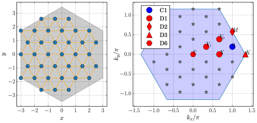
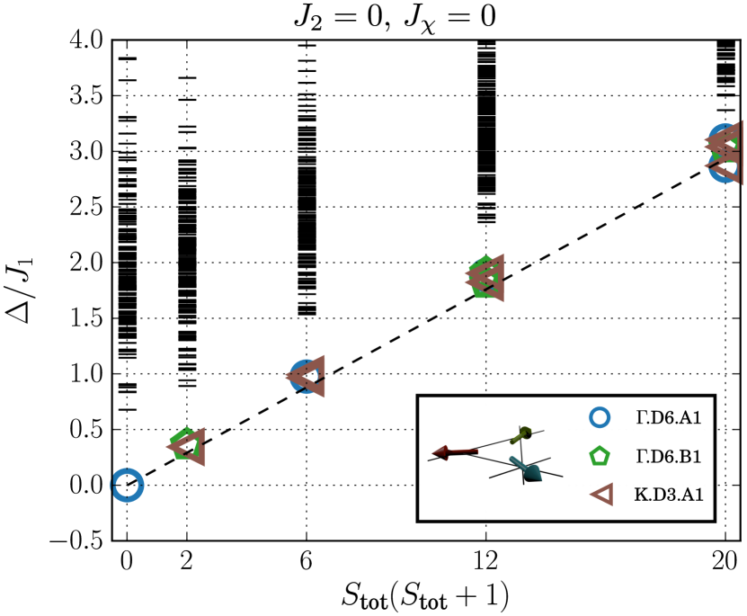
Fig. 4: (Left): Simulation cluster for the Exact Diagonalization calculations. (Center): Brillouin zone of the triangular lattice with the momenta which can be resolved with this choice of the simulation cluster. Different symbols denote the little groups of the corresponding momentum. (Right): TOS for the $120^{\circ}$ Néel order on the triangular lattice. The symmetry sectors and multiplicities fulfill the predictions from the symmetry analysis (See Tab. 5). One should note, that the multiplicities grow with $S_{\text{tot}}$ for non-collinear states.

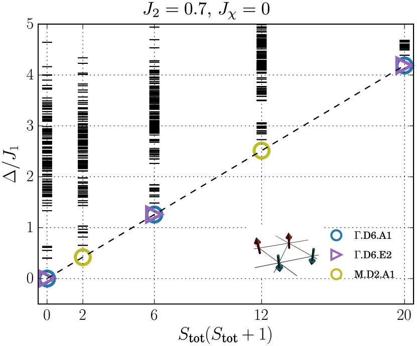
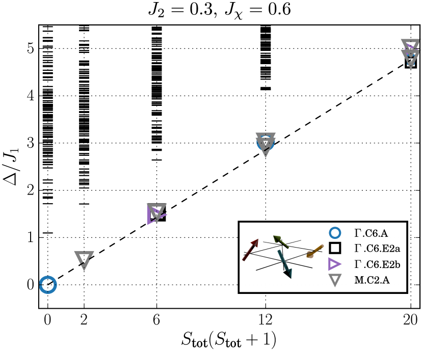
Fig. 5: (Left): TOS for the stripy phase on the triangular lattice. The multiplicities for each even/odd $S_{\text{tot}}$ are constant for collinear phases. (Right): TOS for the tetrahedral order on the triangular lattice.

First of all Fig. 4 shows the simulation cluster used for the Exact Diagonalization calculations in [35]. We chose a $N=36=6\times 6$ sample with periodic boundary conditions. This sample allows to resolve the momenta $\Gamma$, $K$ and $M$, amongst several others in the Brillouin zone. The $K$ and $M$ momenta are the ordering vectors for the $120^{\circ}$, stripy and tetrahedral order. Furthermore, this sample features full sixfold rotational as well as reflection symmetries (the latter only in the absence of the chiral term, i.e. $J_{\chi}=0$). Its pointgroup is therefore given by the dihedral group of order 12, D₆. The little groups of the individual $\mathbf{k}$ vectors are also shown in Fig. 4. For our tower of states analysis we now want to consider the discrete symmetry group

$$\mathcal{D}=\mathcal{T}\times\text{D}_{6}$$ (55)

where $\mathcal{T}$ is the translational group of the magnetic unitcell. The full set of irreducible representations of this symmetry group is given by the set $(\mathbf{k}\otimes\rho_{\mathbf{k}})$ where $\mathbf{k}$ denotes the momentum and $\rho_{\mathbf{k}}$ is an irrep of the little group associated to $\mathbf{k}$. The points $\Gamma$, $K$ and $M$ give rise to the little groups D₆, D₃ and D₂ (the dihedral groups of order $12$, $8$, and $4$), respectively. For the stripy and tetrahedral order we can choose a $2\times 2$ magnetic unitcell, and a $3\times 3$ unitcell for the $120^{\circ}$ Néel order. The spin rotational symmetry gives rise to the continuous symmetry group

$$\mathcal{C}=\text{SO(}3\text{)}$$ (56)

We can therefore label the full set of irreps as $(\mathbf{k},\rho_{\mathbf{k}},S)$ where $S$ denotes the total spin $S$ representation of SO($3$). Similarly to the previous chapter we now want to apply the character-stabilizer formula, Eq. (25), to determine the multiplicities of the representations forming the tower of states. The characters of the irreps $(\mathbf{k},\rho_{\mathbf{k}},S)$ are given by

$$\chi_{(\mathbf{k},\rho_{\mathbf{k}},S)}(t,p,R)=\text{e}^{i\mathbf{k}\cdot\mathbf{t}}\chi_{\rho_{\mathbf{k}}}(p)\frac{\sin\left[(S+\frac{1}{2})\phi\right]}{\sin\frac{\phi}{2}}$$ (57)

where again $\phi\in[0,2\pi]$ is the angle of rotation of the spin rotation $R$.

$\text{D}_{6}$	1	$2C_{6}$	$2C_{3}$	$C_{2}$	$3\sigma_{d}$	$3\sigma_{v}$
A1	1	1	1	1	1	1
A2	1	1	1	1	-1	-1
B1	1	-1	1	-1	1	-1
B2	1	-1	1	-1	-1	1
E1	2	1	-1	-2	0	0
E2	2	-1	-1	2	0	0

Table 4: Character table for pointgroup D₆.

The characters of the pointgroup D₆ are given in Tab. 4. We skip the exact calculations which follow closely the calculations performed in the previous chapter, although now pointgroup symmetries are additionally taken into account. The results are summarized in Tab. 5.

	$120^{\circ}$ Néel				stripy order				tetrahedral order
$S$	$\Gamma$.A1	$\Gamma$.B1	K.A1		$\Gamma$.A1	$\Gamma$.E2	M.A		$\Gamma$.A	$\Gamma$.E2a	$\Gamma$.E2b	M.A
0	1	0	0		1	1	0		1	0	0	0
1	0	1	1		0	0	1		0	0	0	1
2	1	0	2		1	1	0		0	1	1	1
3	1	2	2		0	0	1		1	0	0	2

Table 5: Multiplicities of irreducible representations in the Anderson tower of states for the three magnetic orders on the triangular lattice defined in the main text.

We remark that the tetrahedral order is stabilized only for $J_{\chi}\neq 0$ where the model in Eq. (54) does not have reflection symmetry any more since the term $\mathbf{S}_{i}\cdot(\mathbf{S}_{j}\times\mathbf{S}_{k})$ does not preserve this symmetry. Therefore we used only the pointgroup C₆ of sixfold rotation in the calculations of the tower of states for this phase.

If we compare these results to Figs. 4,5 we see that these are exactly the representations appearing in the TOS from Exact Diagonalization for certain parameter values $J_{2}$ and $J_{\chi}$. This is a strong evidence that indeed SO($3$) symmetry is broken in these models in a way described by the $120^{\circ}$ Néel, stripy and tetrahedral magnetic prototype states.

It is worth noting, that the sum of the multiplicities is constant with $S_{\text{tot}}$ for collinear phases, e.g. the stripy order shown here, whereas it is increasing for non-collinear orders.

4.2.3 Quadrupolar order

All examples of continuous symmetry breaking we have discussed so far spontaneously broke $\text{SO}(3)$ symmetry but exhibited a magnetic moment. In the following we will show examples of phases that do not exhibit any magnetic moment but break spin-rotational symmetry anyway and discuss the influences on the tower of states. We will restrict our discussion to quadrupolar phases in $S=1$ models here, a broader introduction to nematic and multipolar phases can be found in [8].

Quadrupolar states

We denote the basis states for a single spin $S=1$ with $S^{z}=1,-1,0$ as $\ket{1},\ket{\bar{1}},\ket{0}$. In contrast to the usual $S=1/2$ case not each basis state can be obtained by a $\text{SU}(2)$ rotation of any other basis state. The state $\ket{0}$, for example cannot be obtained by a rotation of $\ket{1}$ or $\ket{\bar{1}}$ as it has no orientation in spin-space at all, $\braket{0}{S^{\alpha}}{0}=0$ [8]. The state $\ket{0}$ can, however, be described as a spin fluctuating in the $x-y$ plane in spin space as

$$\braket{0}{(S^{x})^{2}}{0}=\braket{0}{(S^{y})^{2}}{0}=1,\quad\braket{0}{(S^{z})^{2}}{0}=0$$ (58)

We can thus assign a director $\mathbf{d}$ along the $z$-axis to this state. $\text{SU}(2)$ rotations change the director of such a state, but not its property of being non-magnetic. These states are identified as quadrupolar states as they can be detected by utilizing the quadrupolar operator [8]

$$Q^{\alpha\beta}=S^{\alpha}S^{\beta}+S^{\beta}S^{\alpha}-\frac{2}{3}S(S+1)\delta_{\alpha\beta}$$ (59)

To study the possible formation of an ordered quadrupolar phase on a lattice, where the directors of the quadrupoles on each lattice site follow a regular pattern, we consider the bilinear-biquadratic model with Hamiltonian

$$H=\sum_{\langle i,j\rangle}J\;\mathbf{S}_{i}\cdot\mathbf{S}_{j}+Q\left(\mathbf{S}_{i}\cdot\mathbf{S}_{j}\right)^{2}$$ (60)

and $S=1$. The second term in Eq. (60) can be rewritten in terms of the elements of $Q^{\alpha\beta}$ which can be rearranged into a 5-component vector $\mathbf{Q}$ such that

$$\mathbf{Q}_{i}\cdot\mathbf{Q}_{j}=2(\mathbf{S}_{i}\cdot\mathbf{S}_{j})^{2}+\mathbf{S}_{i}\cdot\mathbf{S}_{j}-\frac{4}{3}$$ (61)

The expectation value of Eq. (61) for quadrupolar states on sites $i$ and $j$ is given in terms of their directors $\mathbf{d}_{i,j}$ [8]:

$$\braket{\mathbf{Q}_{i}\cdot\mathbf{Q}_{j}}=2\left(\mathbf{d}_{i}\cdot\mathbf{d}_{j}\right)^{2}-\frac{2}{3}$$ (62)

Therefore, the second term in Eq. (60) favours regular patterns of the directors of quadrupoles. When such states are formed, they spontaneously break $\text{SU}(2)$ symmetry without exhibiting any kind of magnetic moment. The first term in Eq. (60), on the other hand, favours magnetic spin ordering as we have already discussed in previous sections.

The phase diagram of Eq. (60) on the triangular lattice shows extended ferromagnetic, antiferromagnetic ($120^{\circ}$), ferroquadrupolar (FQ) and antiferroquadrupolar (AFQ) ordered phases. In the FQ phase quadrupoles on each lattice site are formed with all directors pointing in a single direction, whereas the directors form a $120^{\circ}$ structure in the AFQ phase. In the following, we will show that the FQ and AFQ phases can be identified and distinguished from the spin ordered phases using the TOS analysis on finite clusters.

TOS for quadrupolar phases

The TOS for the FQ and AFQ phases can be expected to show similar behaviour as the TOS for magnetically ordered states as both spontaneously break the spin-rotational symmetry. If we identify the symmetry-broken quadrupolar phases with their directors pointing in any direction in spin-space we can perform the symmetry analysis of the TOS levels in a very similar manner as for spin-ordered systems in the previous sections. There is, however, one important thing to consider: The directors should not be considered to be described with vectors, but with axes; a quadrupole is recovered (up to a phase) by rotations about an angle $\pi$ around any axis $a$ in the $xy$-plane:

$$\text{e}^{i\pi S^{a}}\ket{0}=-\ket{0}$$ (63)

Thus, the stabilizer in Eq. (25) is different for quadrupolar phases and the TOS shows a different structure. This property makes it possible to distinguish, e.g., a magnetic $120^{\circ}$ phase from its quadrupolar counterpart, the AFQ phase using TOS analysis.

A prototype $\ket{\psi}$ for the FQ phase is a product states of quadrupoles with directors in $z$-direction. This state does not break any space-group symmetries, so only the trivial irreps of the space group, $\mathbf{k}=\Gamma=(0,0),A1$, will be present in the TOS. The remaining stabilizer of the spin-rotation group is a rotation around the $z$-axis about an arbitrary angle and a rotation about an angle $\pi$ around any axis lying in the $xy$-plane,

$$\text{Stab}(\ket{\Psi})=\{R_{z}(\alpha),R_{a}(\pi)\}$$ (64)

The multiplicities in the TOS can then be computed as

$$n_{S} =\frac{1}{2}\left(\frac{1}{|R_{z}(\alpha)|}\int_{0}^{2\pi}d\alpha\chi_{S}(R_{z}(\alpha))+(-1)^{N}\frac{1}{|R_{a}(\pi)|}\int_{0}^{2\pi}da\chi_{S}(R_{a}(\pi))\right)$$ (65)

$$=\frac{1}{2}\left(1+(-1)^{N}(-1)^{S}\right)$$ (66)

where the integrals have already been computed in Eqs. (44) and (45). The system size dependent factor $(-1)^{N}$ is imposed from Eq. (63). To sum up, the TOS for the FQ phase has single levels for even (odd) $S$ with trivial space-group irreps and no levels for odd (even) $S$ sectors when $N$ is even (odd). The absence of odd (even) $S$ levels is caused by the invariance of quadrupoles under $\pi$-rotation and distinguishes the TOS for a FQ phase from a usual ferromagnetic phase. In Fig. 6 the computed TOS for the model Eq. (60) in the FQ phase is shown on the left. It shows the expected quantum numbers and multiplicities in the TOS and also an easily identifiable magnon branch below the continuum.

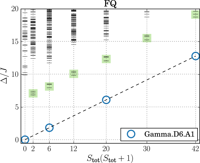
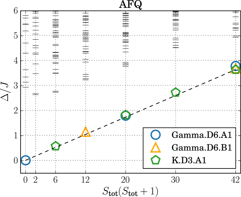
Fig. 6: Tower of states for the ferroquadrupolar (left) and antiferroquadrupolar (right) states on a triangular lattice with $N=12$ sites from Exact Diagonalization. The single-magnon branch for the FQ phase is highlighted with green boxes.

The symmetry analysis for the AFQ phase can be performed in a similar manner and shows a similar structure to the magnetic $120^{\circ}$-Néel phase, but again levels are deleted for the AFQ. In this case, however, not all odd levels are deleted but some levels in both, odd and even, $S$ sectors. Tab. 6 shows the multiplicities of irreps in the TOS of the AFQ model in comparison to the magnetic $120^{\circ}$-Néel state for even $N$. Fig. 6 shows the simulated TOS for the AFQ phase for the bilinear-biquadratic model Eq. (60). The symmetry sectors and multiplicities agree with the predictions.

	AFQ			$120^{\circ}$ Néel
S	$\Gamma$.A1	$\Gamma$.B1	$K$.A1	$\Gamma$.A1	$\Gamma$.B1	$K$.A1
0	1	0	0	1	0	0
1	0	0	0	0	1	1
2	0	0	1	1	0	2
3	0	1	0	1	2	2

Table 6: Irreducible representations and multiplicities for the AFQ phase compared to the magnetic $120^{\circ}$-Néel phase.

5 Outlook

In the previous sections we have discussed prominent features of the energy spectrum for states which spontaneously break the spin-rotational symmetry in the thermodynamic limit. We have seen that on finite-size systems the energy spectra of such states exhibit a tower of states (TOS) structure. The tower of states scales as $S_{\text{tot}}(S_{\text{tot}}+1)/N$ and generates the groundstate manifold in the thermodynamic limit $N\rightarrow\infty$, which is indispensible to spontaneously break a symmetry. The quantum numbers of the levels in the TOS depend on the particular state which is formed after the symmetry breaking and can be predicted using representation theory.
As a generalization to the SU(2)-symmetric Heisenberg model, Eq. (1), one can introduce SU($n$) Heisenberg models with $n>2$. Such models can experimentally be realized by ultracold multicomponent fermions in an optical lattices. When the on-site repulsion is strong enough, the Hamiltonian can be effectively described by an SU($n$) symmetric permutation model on the lattice [36]. If the exchange couplings are antiferromagnetic, SU($n$) generalized versions of the Néel state might be realized as groundstates, which then spontaneously break the SU($n$) symmetry of the Hamiltonian. On finite systems this becomes again manifest in the emergence of a tower of states, where the scaling is found to be proportional to $C_{2}(n)/N$ [37, 38, 39, 40, 36]; $C_{2}(n)$ denotes the quadratic Casimir operator of SU($n$). The symmetry analysis of the levels in the TOS can in principle be performed similar to the case of SO(3) discussed in these notes but the symmetry group and its characters have to be replaced with the more complicated group SU($n$).
On the other side, it can be also interesting to study models where the continuous symmetry group is smaller. In real magnetic materials, the isotropic Heisenberg interaction is often accompanied by other interactions which, when they are strong enough, might reduce the symmetry group of spin rotations to O(2); only spin rotations around an axis are a symmetry of the system and can be spontaneously broken in the thermodynamic limit. This symmetry group is also interesting in the field of ultracold gases, as BECs spontaneously break an O(2) symmetry by choosing a phase. Tower of states can also be found in this case and the quantum numbers and multiplicities of the TOS levels can be computed in a similar fashion [15].

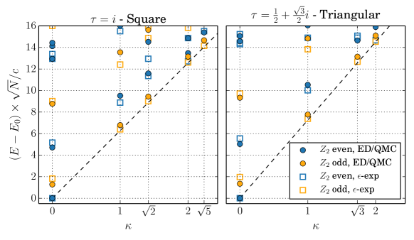
Fig. 7: Universal torus spectrum for a continuous quantum phase transition in the 3D Ising universality class. Full symbols denote numerical results while empty symbols denote $\epsilon$-expansion results. The dashed line shows a dispersion with the speed of light.

We have seen, that the energy spectrum of Hamiltonians on finite lattices may contain a lot of information about the system. One can identify groundstates which will spontaneously break discrete as well as continuous symmetries in the thermodynamic limit and by imposing a classical state as symmetry broken state one can even predict the quantum numbers and multiplicities of the levels in the tower of states or in the quasi-degenerate groundstate manifold. When we impose an additional interaction to a system with spontaneously broken groundstate, e.g. a magnetic field, it is possible that a continuous quantum phase transition (cQPT) from the ordered state to a disordered state appears for some critical ratio of the couplings. Such cQPTs are interesting as they can be described by universal features which do not depend on most microscopic details of the model. Interestingly, the energy spectrum on finite systems can even be used to identify and characterize cQPTs. It is given by universal numbers times $1/L$, where $L=\sqrt{N}$ is the linear size of the lattice. The quantum numbers of the energy levels show universal features and are qualitatively related to the operator content of the underlying critical field theory, although the relation between them is not yet fully understand for non-flat geometries, like a torus [41, 42]. The critical spectrum for the transverse field Ising model on a torus is shown in Fig. 7. It is a fingerprint for the 3D Ising cQPT.

References

-
[1]
P. W. Anderson, Phys. Rev. 86, 694 (1952).
doi:10.1103/PhysRev.86.694
http://link.aps.org/doi/10.1103/PhysRev.86.694 -
[2]
C. Lhuillier, arXiv:cond-mat pp. 161–190 (2005).
doi:10.1007/3-540-45649-X˙6
http://arxiv.org/abs/cond-mat/0502464 -
[3]
A. M. Läuchli: Numerical Simulations of Frustrated Systems
(Springer Berlin Heidelberg, Berlin, Heidelberg, 2011), pp. 481–511.
doi:10.1007/978-3-642-10589-0˙18
http://link.springer.com/10.1007/978-3-642-10589-0_18 -
[4]
A. W. Sandvik, A. Avella, and F. Mancini: In AIP Conf. Proc. (2010),
Vol. 1297, pp. 135–338.
doi:10.1063/1.3518900
http://arxiv.org/abs/1101.3281 -
[5]
H. Suwa and S. Todo, Phys. Rev. Lett. 115, 080601 (2015).
doi:10.1103/PhysRevLett.115.080601
http://link.aps.org/doi/10.1103/PhysRevLett.115.080601 -
[6]
E. Pavarini, E. Koch, J. van den Brink, and G. Sawatzky: Quantum
Materials: Experiments and Theory, Modeling and Simulation, Vol. 6
(Forschungszentrum Jülich, Jülich, 2016)
http://juser.fz-juelich.de/record/819465 -
[7]
G. Misguich and P. Sindzingre, J. Phys. Condens. Matter 19, 145202
(2007).
doi:10.1088/0953-8984/19/14/145202
http://iopscience.iop.org/0953-8984/19/14/145202 -
[8]
K. Penc and A. M. Läuchli: Spin Nematic Phases in Quantum Spin
Systems (Springer Berlin Heidelberg, Berlin, Heidelberg, 2011), pp.
331–362.
doi:10.1007/978-3-642-10589-0˙13
http://link.springer.com/10.1007/978-3-642-10589-0_13 -
[9]
W. Marshall, Proc. R. Soc. A Math. Phys. Eng. Sci. 232, 48 (1955).
doi:10.1098/rspa.1955.0200
http://rspa.royalsocietypublishing.org/cgi/doi/10.1098/%rspa.1955.0200 -
[10]
E. Lieb and D. Mattis, J. Math. Phys. 3, 749 (1962)
http://scitation.aip.org/content/aip/journal/jmp/3/4/10%.1063/1.1724276 -
[11]
A. Auerbach: Interacting Electrons and Quantum Magnetism.
Graduate Texts in Contemporary Physics (Springer New York, New York,
NY, 1994).
doi:10.1007/978-1-4612-0869-3
http://link.springer.com/10.1007/978-1-4612-0869-3 -
[12]
T. A. Kaplan, W. von der Linden, and P. Horsch, Phys. Rev. B 42, 4663
(1990).
doi:10.1103/PhysRevB.42.4663
http://link.aps.org/doi/10.1103/PhysRevB.42.4663 -
[13]
P. Hasenfratz and F. Niedermayer, Zeitschrift f r Phys. B Condens. Matter
92, 91 (1993).
doi:10.1007/BF01309171
http://link.springer.com/10.1007/BF01309171 -
[14]
P. Azaria, B. Delamotte, and D. Mouhanna, Phys. Rev. Lett. 70, 2483
(1993).
doi:10.1103/PhysRevLett.70.2483
http://link.aps.org/doi/10.1103/PhysRevLett.70.2483 -
[15]
I. Rousochatzakis, A. M. Läuchli, and F. Mila, Phys. Rev. B 77,
094420 (2008).
doi:10.1103/PhysRevB.77.094420
http://link.aps.org/doi/10.1103/PhysRevB.77.094420 - [16] R. S. Mulliken, J. Chem.Phys. 23, 1997 (1955). doi:http://dx.doi.org/10.1063/1.1740655
-
[17]
S. Liang, B. Doucot, and P. W. Anderson, Phys. Rev. Lett. 61, 365
(1988).
doi:10.1103/PhysRevLett.61.365
http://link.aps.org/doi/10.1103/PhysRevLett.61.365 -
[18]
C. Lhuillier and G. Misguich: In C. Lacroix, P. Mendels, and F. Mila (Eds.)
Introd. to Frustrated Magn. (Springer Berlin Heidelberg, Berlin,
Heidelberg, 2011), Springer Series in Solid-State Sciences, Vol. 164,
pp. 23–41.
doi:10.1007/978-3-642-10589-0
http://link.springer.com/10.1007/978-3-642-10589-0_2 - [19] E. F. Shender, Sov. Phys. JETP 56, 178 (1982)
-
[20]
C. L. Henley, Phys. Rev. Lett. 62, 2056 (1989).
doi:10.1103/PhysRevLett.62.2056
http://link.aps.org/doi/10.1103/PhysRevLett.62.2056 -
[21]
J. Fouet, P. Sindzingre, and C. Lhuillier, Eur. Phys. J. B 20, 241
(2001).
doi:10.1007/s100510170273
http://link.springer.com/10.1007/s100510170273 -
[22]
A. Läuchli, S. Wessel, and M. Sigrist, Phys. Rev. B 66, 014401
(2002).
doi:10.1103/PhysRevB.66.014401
http://link.aps.org/doi/10.1103/PhysRevB.66.014401 -
[23]
A. Läuchli, J. C. Domenge, C. Lhuillier, P. Sindzingre, and M. Troyer,
Phys. Rev. Lett. 95, 137206 (2005).
doi:10.1103/PhysRevLett.95.137206
http://link.aps.org/doi/10.1103/PhysRevLett.95.137206 -
[24]
M. Mambrini, A. Läuchli, D. Poilblanc, and F. Mila, Phys. Rev. B
74, 144422 (2006).
doi:10.1103/PhysRevB.74.144422
http://link.aps.org/doi/10.1103/PhysRevB.74.144422 -
[25]
A. Gellé, A. M. Läuchli, B. Kumar, and F. Mila, Phys. Rev. B
77, 014419 (2008).
doi:10.1103/PhysRevB.77.014419
http://link.aps.org/doi/10.1103/PhysRevB.77.014419 -
[26]
A. W. Sandvik, Phys. Rev. Lett. 98, 227202 (2007).
doi:10.1103/PhysRevLett.98.227202
http://link.aps.org/doi/10.1103/PhysRevLett.98.227202 -
[27]
T. Senthil, A. Vishwanath, L. Balents, S. Sachdev, and M. P. A. Fisher, Science
(80-. ). 303, 1490 (2004).
doi:10.1126/science.1091806
http://www.sciencemag.org/cgi/doi/10.1126/science.10918%06 -
[28]
T. Jolicoeur, E. Dagotto, E. Gagliano, and S. Bacci, Phys. Rev. B 42,
4800 (1990).
doi:10.1103/PhysRevB.42.4800
http://link.aps.org/doi/10.1103/PhysRevB.42.4800 -
[29]
A. V. Chubukov and T. Jolicoeur, Phys. Rev. B 46, 11137 (1992).
doi:10.1103/PhysRevB.46.11137
http://link.aps.org/doi/10.1103/PhysRevB.46.11137 -
[30]
P. Lecheminant, B. Bernu, C. Lhuillier, and L. Pierre, Phys. Rev. B
52, 6647 (1995).
doi:10.1103/PhysRevB.52.6647
http://link.aps.org/doi/10.1103/PhysRevB.52.6647 -
[31]
Y. Iqbal, W.-J. Hu, R. Thomale, D. Poilblanc, and F. Becca, Phys. Rev. B
93, 144411 (2016).
doi:10.1103/PhysRevB.93.144411
http://link.aps.org/doi/10.1103/PhysRevB.93.144411 -
[32]
R. Kaneko, S. Morita, and M. Imada, J. Phys. Soc. Jpn. 83, 093707
(2014).
doi:10.7566/JPSJ.83.093707
http://journals.jps.jp/doi/10.7566/JPSJ.83.093707 -
[33]
W.-J. Hu, S.-S. Gong, W. Zhu, and D. N. Sheng, Phys. Rev. B 92, 140403
(2015).
doi:10.1103/PhysRevB.92.140403
http://link.aps.org/doi/10.1103/PhysRevB.92.140403 -
[34]
Z. Zhu and S. R. White, Phys. Rev. B 92, 041105 (2015).
doi:10.1103/PhysRevB.92.041105
http://link.aps.org/doi/10.1103/PhysRevB.92.041105 -
[35]
A. Wietek and A. M. Läuchli, Phys. Rev. B 95, 035141 (2017).
doi:10.1103/PhysRevB.95.035141
http://link.aps.org/doi/10.1103/PhysRevB.95.035141 -
[36]
P. Nataf and F. Mila, Phys. Rev. Lett. 113, 127204 (2014).
doi:10.1103/PhysRevLett.113.127204
http://link.aps.org/doi/10.1103/PhysRevLett.113.127204 -
[37]
K. Penc, M. Mambrini, P. Fazekas, and F. Mila, Phys. Rev. B 68, 012408
(2003).
doi:10.1103/PhysRevB.68.012408
http://link.aps.org/doi/10.1103/PhysRevB.68.012408 -
[38]
T. A. Tóth, A. M. Läuchli, F. Mila, and K. Penc, Phys. Rev. Lett.
105, 265301 (2010).
doi:10.1103/PhysRevLett.105.265301
http://link.aps.org/doi/10.1103/PhysRevLett.105.265301 -
[39]
P. Corboz, A. M. Läuchli, K. Penc, M. Troyer, and F. Mila, Phys. Rev.
Lett. 107, 215301 (2011).
doi:10.1103/PhysRevLett.107.215301
http://link.aps.org/doi/10.1103/PhysRevLett.107.215301 -
[40]
P. Corboz, M. Lajkó, K. Penc, F. Mila, and A. M. Läuchli, Phys.
Rev. B 87, 195113 (2013).
doi:10.1103/PhysRevB.87.195113
http://link.aps.org/doi/10.1103/PhysRevB.87.195113 -
[41]
M. Schuler, S. Whitsitt, L.-P. Henry, S. Sachdev, and A. M. Läuchli,
Phys. Rev. Lett. 117, 210401 (2016).
doi:10.1103/PhysRevLett.117.210401
http://link.aps.org/doi/10.1103/PhysRevLett.117.210401 -
[42]
S. Whitsitt and S. Sachdev, Phys. Rev. B 94, 085134 (2016).
doi:10.1103/PhysRevB.94.085134
http://link.aps.org/doi/10.1103/PhysRevB.94.085134
Index
- antiferromagnetism §4.2.1
- bilinear-biquadratic model §4.2.3
- energy spectrum §1
- exact diagonalization §1
- Heisenberg model §2, §4.2.1
- Lieb-Mattis model §2.1
- Néel antiferromagnet §2, §4.2.1
- numerical simulations §1
- order by disorder §4.1.1
- quadrupolar order §4.2.3
- quantum phase transition §5
- representation theory §3.1
- representation theory:irreducible representations §3.2
- representation theory:little group §3.1
- spontaneous symmetry breaking §1
- tetrahedral order §4.2.2
- tower of states §1
- triangular antiferromagnet §4.2.2
- valence bond solid §4.1.1
- valence-bond solid §4.1.1