Gromov width of the disk cotangent bundle of spheres of revolution

Abstract

Inspired by work of the first and second author, this paper studies the Gromov width of the disk cotangent bundle of spheroids and Zoll spheres of revolution. This is achieved with the use of techniques from integrable systems and embedded contact homology capacities.

1 Introduction

Symplectic embedding problems are a central subject in symplectic geometry since Gromov’s nonsqueezing theorem. Among embedding problems, the most basic question is about the largest ball that can be symplectically embedded into a given manifold. More precisely, given a $2n$-dimensional symplectic manifold $(X,\omega)$, its Gromov width $c_{Gr}(X,\omega)$ is defined to be the supremum of $a>0$ such that there exists a symplectic embedding $(B^{2n}(a),\omega_{0})\hookrightarrow(X,\omega)$, where

$$B^{2n}(a)=\left\{(x_{1},y_{1},\dots,x_{n},y_{n})\in{\mathbb{R}}^{2n}\mid\sum_{i=1}^{n}(x_{i}^{2}+y_{i}^{2})\leq a/\pi\right\}\text{ and }\omega_{0}=\sum_{i=1}^{n}dx_{i}\wedge dy_{i}.$$

For any smooth manifold $Q$, its cotangent bundle $T^{*}Q$ has a canonical symplectic structure $\omega_{can}$ which can be written in local coordinates as

$$\omega_{can}=\sum_{i}dp_{i}\wedge dq_{i}.$$

A Riemannian structure on $Q$ gives rise to a norm on the fibers of $T^{*}Q$ and so we can define the disk cotangent bundle $D^{*}Q$ as

$$D^{*}Q=\left\{(q,p)\in T^{*}Q\mid\|p\|<1\right\}.$$

Let $S^{2}\subset{\mathbb{R}}^{3}$ denote the unit sphere endowed with the Riemannian metric induced from ${\mathbb{R}}^{3}$. In [8], the first and second authors showed that

$$c_{Gr}(D^{*}S^{2},\omega_{can})=2\pi.$$

The goal of this article is to generalize this result to spheres of revolution, which are either an ellipsoid or Zoll. We will now explain both cases.

For $a,b,c>0$, let $\mathcal{E}(a,b,c)\subset{\mathbb{R}}^{3}$ be the ellipsoid defined by the equation:

$$\frac{x^{2}}{a^{2}}+\frac{y^{2}}{b^{2}}+\frac{z^{2}}{c^{2}}=1.$$

When the two parameters $a,b$ coincide, we get an ellipsoid of revolution, also called a spheroid. Up to a normalization, we can assume that $a=b=1$. We say that $\mathcal{E}(1,1,c)$ is oblate when $c<1$ and prolate if $c>1$. We also note that $S^{2}=\mathcal{E}(1,1,1)$. In order to state the Gromov width of $D^{*}E(1,1,c)$, we need to use elliptical integrals. We now recall the definition of the complete elliptical integrals of the first, second and third kinds. For $k,n<1$, let

$$K(k) =F\left(\frac{\pi}{2}\Bigm{|}k\right)=\int_{0}^{\pi/2}\frac{d\theta}{\sqrt{1-k\sin^{2}\theta}},$$ (1)

$$E(k) =E\left(\frac{\pi}{2}\Bigm{|}k\right)=\int_{0}^{\pi/2}\sqrt{1-k\sin^{2}\theta}\,d\theta,$$

$$\Pi(n,k) =\Pi\left(n;\frac{\pi}{2}\Bigm{|}k\right)=\int_{0}^{\pi/2}\frac{d\theta}{(1-n\sin^{2}\theta)\sqrt{1-k\sin^{2}\theta}},$$

For each $c<1/2$, let $j_{0}(c)$ be the unique $j\in[0,1]$ such that

$$-jcK\left(\frac{(c^{2}-1)(1-j^{2})}{c^{2}}\right)+\frac{j}{c}\Pi\left(\frac{c^{2}-1}{c^{2}},\frac{(c^{2}-1)(1-j^{2})}{c^{2}}\right)=\frac{\pi}{4}.$$ (2)

It follows from the Intermediate Value Theorem that (2) has a solution for a fixed $c<1/2$. We will see in the proof of Lemma 2.8 that this solution is unique. Now let

$$\alpha(c) =8cE\left(\frac{(c^{2}-1)(1-j_{0}(c))}{c^{2}}\right),\text{ for }c<1/2,$$

$$\beta(c) =4E(1-c^{2}).$$

Remark 1.1.

The number $\beta(c)$ is simply the length of any meridian of $\mathcal{E}(1,1,c)$. We will see in Section 2.2 that $\alpha(c)$ is the length of a simple geodesic on $\mathcal{E}(1,1,c)$ that intersects the equator 4 times and only exists when $c<1/2$.

We also let $c_{0}$ denote the value of $c$ for which $\beta(c)=4\pi$. It follows from a simple numerical calculation that $2<c_{0}<3$. We can now state the main result of this paper.

Theorem 1.2.

The Gromov width of $D^{*}\mathcal{E}(1,1,c)$ is given by

$$c_{Gr}(D^{*}\mathcal{E}(1,1,c),\omega_{can})=\left\{\begin{aligned} \alpha(c),&\text{ for }0<c<1/2,\\ 2\pi,&\text{ for }1/2\leq c\leq 1,\\ \beta(c),&\text{ for }1<c<c_{0},\\ 4\pi,&\text{ for }c\geq c_{0}.\end{aligned}\right.$$

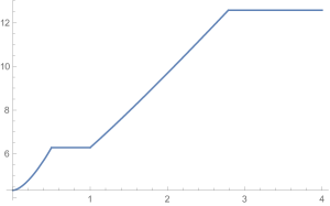
Figure 1: The graph of function $c\mapsto c_{Gr}(D^{*}\mathcal{E}(1,1,c),\omega_{can})$.

The proof of Theorem 1.2 has two parts. We will first find a toric domain that symplectically embeds into $D^{*}\mathcal{E}(1,1,c)$ filling its volume and we will find a ball embedding into this toric domain. Then we will use embedded contact homology (ECH) capacities to show that we cannot do better than that.

Now recall that a Riemannian manifold is said to be Zoll if all geodesics are closed and have the same length. Our second result is the following.

Theorem 1.3.

Let $S$ be a Zoll sphere of revolution and $\ell$ be the length of any simple closed geodesic. Then

$$c_{Gr}(D^{*}S,\omega_{can})=\ell.$$

The proof of Theorem 1.3 is similar to Theorem 1.2. Using the integrability of the geodesic flow, we can find an embbeded ball in the disk cotangent bundle of more general spheres of revolution, obtaining a lower bound for the Gromov width for a larger class of spheres of revolution. The upper bound in the Zoll case is again obtained by ECH capacities.

1.1 A toric domain in disguise

A four-dimensional toric domain is a subset of ${\mathbb{C}}^{2}$ defined by

$$\mathbb{X}_{\Omega}=\left\{(z_{1},z_{2})\in{\mathbb{C}}^{2}\mid(\pi|z_{1}|^{2},\pi|z_{2}|^{2})\in\Omega\right\},$$

where $\Omega\subset{\mathbb{R}}_{\geq 0}^{2}$ is the closure of an open set in ${\mathbb{R}}^{2}$. Now suppose that $\Omega$ is the region bounded by the coordinate axes and a piecewise smooth curve $\gamma$ connecting $(a,0)$ to $(0,b)$ for some $a,b>0$. A toric domain $\mathbb{X}_{\Omega}$ is said to be

1. concave, if $\gamma$ is the graph of a convex function $[0,a]\to{\mathbb{R}}_{\geq 0}$;

2. convex, if $\gamma$ is the graph of a concave function $[0,a]\to{\mathbb{R}}_{\geq 0}$;

3. weakly convex, if $\gamma$ is a convex curve.

The first step in the proof of Theorem 1.2 is to find a toric domain that symplectically embeds into $D^{*}\mathcal{E}(1,1,c)$. More precisely, we use the main idea of [13] as in [8], to prove that the complement of the fiber over $(0,0,c)$ is symplectomorphic to the interior of a toric domain. It turns out that this actually holds in a more general setting.

Let $S\subset{\mathbb{R}}^{3}$ be a sphere of revolution, meaning that $S$ is a genus zero compact smooth surface, which is invariant under rotation around a fixed coordinate axis. Without loss of generality, we can assume that $S$ has the form

$$S=\{((u(z)\cos\theta,u(z)\sin\theta,z)\mid z\in[a,b],\theta\in{\mathbb{R}}/2\pi{\mathbb{Z}}\},$$ (3)

where $u(z)>0$ for $z\neq a,b$, and $u(a)=u(b)=0$. We define the north and south poles by $P_{N}=(0,0,b)$ and $P_{S}=(0,0,a)$, respectively. An equator is a circle $C=\{(x,y,z)\in S\mid z=z_{0}\}$, whenever $z_{0}$ is a critical point of $u$.

Theorem 1.4.

Let $S\subset\mathbb{R}^{2}$ be a sphere of revolution with a unique equator. Then there exists a toric domain $\mathbb{X}_{\Omega_{S}}$ such that $(D^{*}(S\backslash\{P_{N}\}),\omega_{can})$ is symplectomorphic to $(\operatorname{int}\mathbb{X}_{{\Omega}_{S}},\omega_{0})$.

For the case of Zoll spheres of revolution we can go further and give the precise toric domain found in Theorem 1.4.

Proposition 1.5.

Let $S\subset\mathbb{R}^{2}$ be a Zoll sphere of revolution and $\ell$ be the length of any simple closed geodesic. Then $(D^{*}(S\backslash\{P_{N}\}),\omega_{can})$ is symplectomorphic to the symplectic bidisk $(\operatorname{int}B^{2}(\ell)\times B^{2}(\ell),\omega_{0})$.

We can do this also for the ellipsoids of revolution, as well as analyze the convexity/concavity of the corresponding toric domain.

Proposition 1.6.

For each $c>0$, $(D^{*}(\mathcal{E}(1,1,c)\backslash\{(0,0,c)\}),\omega_{can})$ is symplectormorphic to $(\operatorname{int}\mathbb{X}_{\Omega_{c}},\omega_{0})$, where $\mathbb{X}_{\Omega_{c}}$ is a toric domain which is:

1. neither concave nor weakly convex for $c<1$,

2. weakly convex for $c\geq 1$.

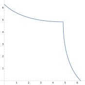
(a) $c=0.5$

(b) $c=1$

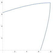
(c) $c=1.5$

Figure 2: The region $\Omega_{c}$ for different values of $c$.

Remark 1.7.

For $c=1$ we recover the result in [8] stating that the disk cotangent bundle of the round sphere minus a point is symplectomorphic to the symplectic bidisk $\operatorname{int}B^{2}(2\pi)\times B^{2}(2\pi)$.

The next step in the proof of Theorem 1.2 is the construction of the embedding of an appropriate ball into $\mathbb{X}_{\Omega_{c}}$. Let

$$w(c):=\left\{\begin{aligned} \alpha(c),&\text{ for }0<c<1/2,\\ 2\pi,&\text{ for }1/2\leq c\leq 1,\\ \beta(c),&\text{ for }1<c<c_{0},\\ 4\pi,&\text{ for }c\geq c_{0}.\end{aligned}\right.$$ (4)

Proposition 1.8.

For every $c>0$, there exists a symplectic embedding

$$\left(\operatorname{int}B^{4}(w(c)),\omega_{0}\right)\hookrightarrow\left(\operatorname{int}\mathbb{X}_{\Omega_{c}},\omega_{0}\right).$$

As we will see in Section 2.3, this embedding is just the inclusion for $c\leq 1$. On the other hand, for $c>1$ we will need to use Cristofaro–Gardiner’s highly nontrivial construction of a symplectic embedding from a concave into a weakly convex toric domain.

The last ingredient in the proof of Theorem 1.2 is the calculation of some ECH capacities of $(D^{*}\mathcal{E}(1,1,c),\omega_{can})$. We recall that ECH capacities are a sequence of symplectic capacities four-dimensional symplectic manifold. In particular,

$$(X_{1},\omega_{1})\hookrightarrow(X_{2},\omega_{2})\Rightarrow c_{k}(X_{1},\omega_{1})\leq c_{k}(X_{2},\omega_{2})\;\text{ for every }k.$$

Proposition 1.9.

1. $c_{3}\left(D^{*}\mathcal{E}(1,1,c),\omega_{can}\right)=2w(c)$, for $0<c<c_{0}$,

2. $c_{1}\left(D^{*}\mathcal{E}(1,1,c),\omega_{can}\right)=4\pi$, for $c\geq 1$.

Using Propositions 1.6, 1.8 and 1.9, we can prove our main theorem.

Proof of Theorem 1.2.

It follows from Propositions 1.8 and 1.6 that for any $\varepsilon>0$, there exists a symplectic embedding

$$B^{4}\left((1-\varepsilon)w(c)\right)\hookrightarrow\left(D^{*}\mathcal{E}(1,1,c),\omega_{can}\right).$$

So $c_{Gr}\left(D^{*}\mathcal{E}(1,1,c),\omega_{can}\right)\geq(1-\varepsilon)w(c)$ for every $\varepsilon>0$ and hence

$$c_{Gr}\left(D^{*}\mathcal{E}(1,1,c),\omega_{can}\right)\geq w(c).$$

Now suppose that $(B^{4}(a),\omega_{0})\hookrightarrow\left(D^{*}\mathcal{E}(1,1,c),\omega_{can}\right)$. Recall that $c_{1}(B^{4}(a))=a$ and $c_{3}(B^{4}(a))=2a$. For $c<c_{0}$, it follows from Proposition 1.9(a) that

$$2a=c_{3}(B^{4}(a))\leq c_{3}\left(D^{*}\mathcal{E}(1,1,c),\omega_{can}\right)=2w(c).$$

For $c\geq c_{0}$, Proposition 1.9(b) implies that

$$a=c_{1}(B^{4}(a))\leq c_{1}\left(D^{*}\mathcal{E}(1,1,c),\omega_{can}\right)=4\pi=w(c).$$

So in either case $a\leq w(c)$. Taking the supremum on $a$, we conclude that

$$c_{Gr}\left(D^{*}\mathcal{E}(1,1,c),\omega_{can}\right)\leq w(c).$$

∎

Structure of the paper: In Section 2 we use techniques from integrable systems to construct toric domains in the disk cotangent bundles of spheres of revolution. In particular, we prove Theorem 1.4, Propositions 1.5 and 1.6. In Section 3 we recall what we need from ECH and we compute some ECH capacities, allowing us to prove Propositions 1.8, 1.9 and Theorem 1.3.

Acknowledgements: The second author is partially supported by grants from the Serrapilheira Insitute, CNPq and FAPERJ.

2 Toric domains in the disk cotangent bundles of spheres of revolution

2.1 Integrability of geodesic flow

Let $S\subset\mathbb{R}^{3}$ be a sphere of revolution as in (3). We endow $S$ with the metric induced by the ambient Euclidean space ${\mathbb{R}}^{3}$ and denote it by $\langle\cdot,\cdot\rangle$. Further, we denote the induced norm by $\lVert\cdot\rVert$. It is well known that the meridians, namely, any intersection of $S$ with a plane containing the $z$-axis, are closed geodesics of $S$. The same hold for the equators, see e.g. [11, Proposition 3.5.22].

The goal of this section is to show that if $S$ has a unique equator then $D^{*}S$ is the union of two copies of a toric domain and a measure zero set. We do this by using the integrability of the geodesic flow on spheres of revolution following ideas from [16]. As a first consequence, one can study the geodesic flow of $S$ by studying the Reeb flow on the boundary of the corresponding toric domain. Further, we find symplectically embedded balls in the disk cotangent bundle $D^{*}S$ of $S$ under a twisting hypothesis using the Traynor trick described in [15, $\S 5$].

Assume $S$ has a unique equator. We first consider the energy function

$$H\colon T^{*}S \to {\mathbb{R}}$$

$$(q,p) \mapsto \lVert p\rVert^{2}.$$

The Hamiltonian flow of $H$ is a reparametrization of the cogeodesic flow defined on $T^{*}S$. Here, by cogeodesic flow we mean the flow associated to the vector field which is dual to the geodesic vector field via the bundle isomorphism given by the metric

$$\langle\cdot,\cdot\rangle^{\flat}\colon TS \to T^{*}S$$ (5)

$$X \mapsto \langle X,\cdot\rangle.$$

It is well known that the angular momentum is an integral of motion for the Hamiltonian system defined by the energy. To define this function, consider the vector field $\partial_{\theta}=-y\partial_{x}+x\partial_{y}$ defined in Cartesian coordinates, that is, the vector field on $S$ that generates the rotations around the $z$-axis. We can define the angular momentum $J$ by

$$J\colon T^{*}S \to {\mathbb{R}}$$

$$(q,p) \mapsto p(\partial_{\theta}).$$

We will now use the fact that $(H,J)$ is an integrable system to find action-angle coordinates. Moreover, we obtain strict contactomorphisms as stated in the theorem below.

Theorem 2.1.

Let $S$ be a sphere of revolution with only one equator and consider $F=(H,J)|_{D^{*}S}\colon D^{*}S\to{\mathbb{R}}$, where $H$ is the energy and $J$ is the angular momentum. Then the set of regular points of $F$ has two connected components $U_{+},U_{-}$ corresponding to where $J$ is positive or negative, respectively. These components are symplectomorphic to a toric domain. Moreover, the symplectomorphisms restrict to strict contactomorphisms on the boundaries $\partial U_{+},\partial U_{-}\subset S^{*}S$.

Proof.

The coordinates $(z,\theta)$ on $S$ induce cotangent coordinates $(z,\theta,p_{z},p_{\theta})$ on $T^{*}S$. In these coordinates, it follows from a simple calculation that

$$H(z,\theta,p_{z},p_{\theta})=\frac{p_{z}^{2}}{u^{\prime}(z)^{2}+1}+\frac{p_{\theta}^{2}}{u(z)^{2}},\quad J(z,\theta,p_{z},p_{\theta})=p_{\theta}.$$

In particular, $H$ and $J$ Poisson commute, i.e., $\{H,J\}=0$. Since

$$J(q,p)^{2}=\langle p^{*},\partial_{\theta}\rangle^{2}\leq\lVert p^{*}\rVert^{2}\lVert\partial_{\theta}\rVert^{2}=H(q,p)u(z)^{2},$$

we have $|J(q,p)|\leq u(z_{0})\sqrt{H(q,p)}$, for all $p\in T^{*}S$. Here we denote by $p^{*}$ the tangent vector dual to $p$ via the vector bundle isomorphism (5) and $z_{0}\in(a,b)$ is the unique critical point of $u$, where $u$ attains its maximum. The image of $F=(H,J)$ restricted to $D^{*}S$ is given by

$$B:=\{(h,j)\in{\mathbb{R}}^{2}\mid 0\leq h\leq 1\ \text{and}\ |j|\leq u(z_{0})\sqrt{h}\}.$$ (6)

The critical points of $F$ are the points $(q,p)$ such that one of the following conditions is satisfied:

• $p=0$ (the zero-section),

• $q=P_{S}$ or $q=P_{N}$ (the fibers over the poles),

• $z=z_{0}$ and $p_{z}=0$ (the equator with either orientation).

Hence, $B$ is the region bounded by the parabola $u(z_{0})^{2}h=j^{2}$ and by the line $h=1$, and the critical values of $F$ are exactly the points on this parabola and on the horizontal line $j=0$. Now we apply the classical Arnold–Liouville Theorem in a subset of $D^{*}S$. Let

$$B_{+}:=\{(h,j)\in{\mathbb{R}}^{2}\mid 0<h\leq 1\ \text{and}\ 0<j<u(z_{0})\sqrt{h}\}.$$

We define two families of circles $\gamma_{1}^{(h,j)}$ and $\gamma_{2}^{(h,j)}$ generating $H_{1}(F^{-1}(h,j);{\mathbb{Z}})$ and depending smoothly on $(h,j)\in B_{+}$. Let

$$\gamma_{1}^{(h,j)} =\{(z,\theta,p_{z},p_{\theta})\in F^{-1}(h,j)\mid z=z_{0},p_{z}>0\},$$

$$\gamma_{2}^{(h,j)} =\{(z,\theta,p_{z},p_{\theta})\in F^{-1}(h,j)\mid\theta=0\}.$$

Then $\gamma_{1}^{(h,j)}$ and $\gamma_{2}^{(h,j)}$ are families of simple closed curves generating $H_{1}(F^{-1}(h,j);{\mathbb{Z}})$. Let $\lambda=p_{\theta}\,d\theta+p_{z}\,dz$ be the tautological form on $T^{*}S$. In particular, $d\lambda=\omega_{can}$. The action coordinates are defined by

$$I_{1}(h,j) =\int_{\gamma_{1}^{(h,j)}}\lambda=2\pi j,$$ (7)

$$I_{2}(h,j) =\int_{\gamma_{2}^{(h,j)}}\lambda=2\int_{z_{-}(h,j)}^{z_{+}(h,j)}\sqrt{\left(h-\frac{j^{2}}{u(z)^{2}}\right)(u^{\prime}(z)^{2}+1)}\,dz,$$ (8)

where $z_{-}(h,j)<z_{+}(h,j)$ are the two solutions to the equation $u(z)^{2}h-j^{2}=0$. We observe that the map $\varphi=(I_{1},I_{2}):B_{+}\to{\mathbb{R}}^{2}$ is a smooth embedding. Its image, which we denote by $\Omega$ is the region in ${\mathbb{R}}^{2}_{>0}$ bounded by the curve parametrized by

$$\gamma(j)=\left(2\pi j,2\int_{z_{-}(1,j)}^{z_{+}(1,j)}\sqrt{\left(1-\frac{j^{2}}{u(z)^{2}}\right)(u^{\prime}(z)^{2}+1)}\,dz\right)$$ (9)

for $j\in[0,u(z_{0})]$. Let $U_{+}=F^{-1}(B_{+})$. It follows from the Arnold-Liouville theorem that there exists a symplectomorphism $\Phi\colon(U_{+},\omega_{can})\to(\mathbb{X}_{\Omega},\omega_{0})$, such that the diagram commutes

where $\mu(z_{1},z_{2})=(\pi|z_{1}|^{2},\pi|z_{2}|^{2})$ is the standard moment map.

We now show that $\Phi$ can be chosen so that $\Phi^{*}\lambda_{0}=\lambda$, where $\lambda_{0}$ is the standard Liouville form on ${\mathbb{C}}^{2}$. Following Arnold [2], we can find angle coordinates using generating functions as follows. First, note that our primitive $\lambda$ is closed on the Lagrangian torus $F^{-1}(h,j)$ since $d\lambda|_{F^{-1}(h,j)}=\omega_{can}|_{F^{-1}(h,j)}=0$. For $(q,p)=(z,\theta,p_{z},j)\in F^{-1}(h,j)$, we let $\gamma_{(q,p)}$ be a smooth path on $F^{-1}(B_{+})$ from $(q_{0},p_{0}):=(z_{-}(h,j),0,0,j)$ to $(q,p)$. We define the multivalued function $G$ by

$$G(q,p)=\int_{\gamma_{(q,p)}}\lambda.$$

The angle coordinates are heuristically defined by

$$\phi_{1}=\frac{\partial G}{\partial I_{1}},\quad\phi_{2}=\frac{\partial G}{\partial I_{2}}.$$ (10)

More precisely, given a diffeomorphism $\psi:({\mathbb{R}}^{2}/{\mathbb{Z}}^{2})\times B_{+}\to U_{+}$ such that $\psi(0,0,h,j)=(z_{-}(h,j),0,0,j)$, we consider a lift $\widetilde{\psi}:{\mathbb{R}}^{2}\times B_{+}\to U_{+}$ and we define a function

$$\widetilde{G}(t,(h,j))=\int_{(0,(h,j))}^{(t,(h,j))}\widetilde{\psi}^{*}\lambda,$$

where the integral above is over a path contained in ${\mathbb{R}}^{2}\times\{(h,j)\}$. Then $\widetilde{G}$ can be seen as a well-defined lift of $G$. Note that $\widetilde{G}$ is independent of the choice of lift $\widetilde{\psi}$. The angle coordinates are defined by

$$\phi_{1}(q,p) =\frac{\partial(\widetilde{G}\circ(\text{id}\times\varphi^{-1}))}{\partial I_{1}}(t,\varphi(h,j)),$$ (11)

$$\phi_{2}(q,p) =\frac{\partial(\widetilde{G}\circ(\text{id}\times\varphi^{-1}))}{\partial I_{2}}(t,\varphi(h,j))$$

where $\widetilde{\psi}(t,(h,j))=(q,p)$. We observe that the partial derivatives above are independent of the choice of the preimage $\widetilde{\psi}^{-1}(q,p)$ so they can be seen as partial derivatives of $G$. So (10) can be seen as a simplified expression for (11).

As usual, we define

$$\Phi\colon U_{+}\to X_{\Omega},\qquad(q,p)\mapsto\left(\sqrt{\frac{I_{1}(q,p)}{\pi}}e^{2\pi\phi_{1}(q,p)},\sqrt{\frac{I_{2}(q,p)}{\pi}}e^{2\pi\phi_{2}(q,p)}\right)$$

It is well-known that $\Phi$ is a symplectomorphism, see [2]. We now prove that $\Phi^{*}\lambda_{0}=\lambda$. Taking polar coordinates in each complex variable of ${\mathbb{C}}^{2}$, we can write

$$\lambda_{0}=\frac{1}{2}\sum_{i=1}^{2}r_{i}^{2}\,d\theta_{i}.$$

So

$$\Phi^{*}\lambda_{0}=I_{1}\,d\phi_{1}+I_{2}\,d\phi_{2}.$$

Claim: $I_{1}\,d\phi_{1}+I_{2}\,d\phi_{2}=\lambda$.

Proof of the Claim.

Let $(q,p)=(z,\theta,p_{z},p_{\theta})$ such that $p_{z}\neq 0$ and let $(h,j)=F(q,p)$. We choose a preimage $(t,(h,j))\in\widetilde{\psi}^{-1}(q,p)$ such that the $p_{z}$-coordinate of $\widetilde{\psi}(s,F(q,p))$ does not vanish for $0<s\leq t$. Let

$$P(w,h,j):=\sqrt{\left(h-\frac{j^{2}}{u(w)^{2}}\right)(u^{\prime}(w)^{2}+1)}.$$ (12)

So $\widetilde{G}(t,(h,j))=\widetilde{G}(z,\theta,h,j)$ is given by

$$\widetilde{G}(z,\theta,h,j)=\sigma\int_{z_{-}(h,j)}^{z}P(w,h,j)\,dw+\theta j,$$ (13)

where $\sigma\in\{-1,1\}$ is the sign of $p_{z}$. We note that (13) holds in a neighborhood of $(t,(h,j))$. By slightly abusing notation, we write $(h,j):=\varphi^{-1}(I_{1},I_{2})$. It follows from (7), (8) and (12) that

$$\frac{\partial h}{\partial I_{1}} =-\frac{\int_{z_{-}(h,j)}^{z_{+}(h,j)}\partial_{j}P(w,h,j)\,dw}{2\pi\int_{z_{-}(h,j)}^{z_{+}(h,j)}\partial_{h}P(w,h,j)\,dw}, \frac{\partial j}{\partial I_{1}} =\frac{1}{2\pi},$$ (14)

$$\frac{\partial h}{\partial I_{2}} =\frac{1}{2\int_{z_{-}(h,j)}^{z_{+}(h,j)}\partial_{h}P(w,h,j)\,dw}, \frac{\partial j}{\partial I_{2}} =0.$$

Using (7), (8), (11), (12) and (14), we compute the angle coordinates:

$$\phi_{1}(z,\theta,h,j) =-\frac{\sigma\int_{z_{-}(h,j)}^{z}\partial_{h}P(w,h,j)\,dw\cdot\int_{z_{-}(h,j)}^{z_{+}(h,j)}\partial_{j}P(w,h,j)\,dw}{2\pi\int_{z_{-}(h,j)}^{z_{+}(h,j)}\partial_{h}P(w,h,j)\,dw}$$ (15)

$$+\frac{\sigma}{2\pi}\int_{z_{-}(h,j)}^{z}\partial_{j}P(w,h,j)\,dw+\frac{\theta}{2\pi},$$

$$\phi_{2}(z,\theta,h,j) =\frac{\sigma\int_{z_{-}(h,j)}^{z}\partial_{h}P(w,h,j)\,dw}{2\int_{z_{-}(h,j)}^{z_{+}(h,j)}\partial_{h}P(w,h,j)\,dw}.$$

It follows from (12) that

$$P=j\partial_{j}P+2h\partial_{h}P.$$ (16)

From (15) and (16), we obtain

$$I_{1}(h,j)\phi_{1}(z,\theta,h,j) =2\pi j\phi_{1}(z,\theta,h,j)$$ (17)

$$=-I_{2}(h,j)\phi_{2}(z,\theta,h,j)+\sigma\int_{z_{-}(h,j)}^{z}P(w,h,j)\,dw+\theta j.$$

It follows from (13) and (17) that

$$I_{1}\phi_{1}+I_{2}\phi_{2}=\widetilde{G}.$$

Differentiating this equation and using (11) and (13) we obtain

$$I_{1}\,d\phi_{1}+I_{2}\,d\phi_{2}+\phi_{1}\,dI_{1}+\phi_{2}\,dI_{2} =\sigma P\,dz+j\,d\theta+\partial_{I_{1}}\widetilde{G}\,dI_{1}+\partial_{I_{2}}\widetilde{G}\,dI_{2}$$

$$=p_{z}\,dz+p_{\theta}\,d\theta+\phi_{1}\,dI_{1}+\phi_{2}\,dI_{2}.$$

Therefore $I_{1}\,d\phi_{1}+I_{2}\,d\phi_{2}=\lambda$ proving the claim whenever $p_{z}\neq 0$. By continuity, this equation also holds when $p_{z}=0$. ∎

We conclude that the symplectomorphism $\Phi$ restricts to a strict contactomorphism $\Phi|_{\partial U_{+}}$ between $\partial U_{+}$ and $\partial\mathbb{X}_{\Omega}$. Analogously, one can reproduce the argument above to the symmetric set $U_{-}:=F^{-1}(B_{-})$, where

$$B_{-}:=\{(h,j)\mid 0<h\leq 1\ \text{and}\ -u(r_{0})\sqrt{h}<j<0\},$$

and conclude the same thing, i.e., $U_{-}$ is symplectomorphic to $\mathbb{X}_{\Omega}$ and the symplectomorphism restricts to a strict contactomorphism between the boundaries. In particular, $U_{+}$ and $U_{-}$ are symplectomorphic. ∎

Remark 2.2.

Using theorems of Eliasson [6, 7] as done in [13] and [12], we can extend the symplectomorphisms above to the sets

$$\{(h,j)\in{\mathbb{R}}^{2}\mid 0<h\leq 1\text{ and }0<j\leq u(z_{0})\sqrt{h}\},$$

$$\{(h,j)\in{\mathbb{R}}^{2}\mid 0<h\leq 1\text{ and }-u(z_{0})\sqrt{h}\leq j<0\}.$$

By continuity, we also have $\Phi^{*}\lambda_{0}=\lambda$ for these two sets (including $h=1$). But we cannot extend them for $j=0$.

Let $\mathfrak{m}=\min\{2\pi u(z_{0}),L\}$, with $L$ denoting the length of any meridian on $S$. In other words, $\mathfrak{m}$ is the minimum between the length of the equator and the length of a meridian on $S$. It is readily verified from equation (9) that the curve $\gamma$ is the graph of a function $f_{S}$ defined by

$$f_{S}\colon[0,2\pi u(z_{0})] \to [0,\mathfrak{m}]$$

$$j \mapsto 2\int_{z_{-}(1,j)}^{z_{+}(1,j)}\sqrt{\left(1-\frac{j^{2}}{4\pi^{2}u(z)^{2}}\right)(u^{\prime}(z)^{2}+1)}\,dz,$$

Moreover, note that $f_{S}$ satisfies $f_{S}(0)=L$ and $f_{S}(2\pi u(z_{0}))=0$. In particular, if $f_{S}$ is concave or convex, the open triangle

$$\bigtriangleup(\mathfrak{m})=\{(x,y)\in{\mathbb{R}}_{>0}^{2}\mid x+y<\mathfrak{m}\},$$

is contained in $\Omega$. Therefore, we apply the Traynor trick to obtain the following result.

Proposition 2.3.

Suppose that $S$ has only one equator and that the function $f_{S}$ is a concave or convex function. Let $\mathfrak{m}=\min\{2\pi u(s_{0}),L\}$. Then, there exists a symplectic embedding

$$(\operatorname{int}(B(\mathfrak{m})),\omega_{0})\hookrightarrow(D^{*}S,\omega_{can}).$$

In particular, $c_{Gr}((D^{*}S,\omega_{can})\geq\mathfrak{m}$.

Remark 2.4.

1. The discussion above can be adapted to the case where $S$ has more than one equator. In this case, it is possible to conclude that the Gromov width of $(D^{*}S,\omega_{can})$ is at least the minimum between the length of the smallest equator of $S$ and the length of a meridian.

2. The derivative of the function $f_{S}$ is directly related to the equatorial first return angle defined by Zelditch, see [16]. In this case, one can prove that the convexity of $f_{c}$ is related to a twisting condition on the (non-linear) Poincaré map for the equator.

Example 2.5 (Round sphere).

The round sphere $S^{2}\subset{\mathbb{R}}^{3}$ is described by the function $u(z)=\sqrt{1-z^{2}}$, for $z\in[-1,1]$. In this case, Proposition 2.3 ensures the existence of a symplectic embedding

$$(\operatorname{int}(B(2\mathfrak{\pi})),\omega_{0})\hookrightarrow(D^{*}S,\omega_{can}).$$

In fact, the first two named authors showed in [8] that $(\operatorname{int}(B(2\mathfrak{\pi})),\omega_{0})$ is symplectomorphic to $(\operatorname{int}D^{*}\Sigma,\omega_{can})$, where $\Sigma$ is any open hemisphere in the sphere $S^{2}$.

2.2 Toric domains hidden in spheres of revolution

In this section we prove Theorem 1.4. To do that we will use a perturbed version of the integrable system appearing in the proof of Theorem 2.1.

Proof of Theorem 1.4.

We use the same notation as the proof of Theorem 2.1. Let $0<\varepsilon<b-z_{0}$ and let $U_{\varepsilon}\in C^{\infty}([0,b-\varepsilon))$ be a non-decreasing smooth function supported in $(z_{0},b-\varepsilon)$, such that $U_{\varepsilon}(z)=\frac{\varepsilon}{b-\varepsilon-z}$ for $z$ sufficiently close to $b-\varepsilon$. We also assume that the family $U_{\varepsilon}$ is increasing in $\varepsilon$. For $(q,p)=(z,\theta,p_{z},p_{\theta})\in D^{*}S$ such that $z<b-\varepsilon$, we define

$$H^{\varepsilon}(z,\theta,p_{z},p_{\theta})=H(z,\theta,p_{z},p_{\theta})+U_{\varepsilon}(z).$$

Note that $H^{\varepsilon}$ does not depend on $\theta$ and so it still Poisson commutes with $J$. Now let $F^{\varepsilon}=(H^{\varepsilon},J)$ whose domain is

$$W^{\varepsilon}:=\{(z,\theta,p_{z},p_{\theta})\in D^{*}S\mid H^{\varepsilon}(z,\theta,p_{z},p_{\theta})\leq 1\}.$$

It follows from the assumptions on $U_{\varepsilon}$ that $F^{\varepsilon}(W^{\varepsilon})=B$, as defined in (6) and that $(h,j)$ is a critical value of $F^{\varepsilon}$ if, and only if $|j|=u(z_{0})\sqrt{h}$. In particular if $j=0$ and $h\neq 0$, then $(h,j)$ is not a critical value of $F^{\varepsilon}$. So we can apply the Arnold-Liouville theorem in

$$\operatorname{int}(B)=\{(h,j)\in{\mathbb{R}}^{2}\mid 0<h<1,\,|j|<u(z_{0})\sqrt{h}\}.$$

So there exists a domain $\Omega^{\varepsilon}\subset{\mathbb{R}}^{2}_{>0}$, a diffeomorphism $\varphi^{\varepsilon}:\operatorname{int}(B)\to\Omega^{\varepsilon}$ and a symplectomorphism $\Phi^{\varepsilon}:(F^{\varepsilon})^{-1}(\operatorname{int}(B))\to\mathbb{X}_{\Omega^{\varepsilon}}$ such that the following diagram commutes.

As in Section 2.1, we need to choose two smooth families of loops $\{\gamma_{1}^{(h,j)},\gamma_{2}^{(h,j)}\}\subset(F^{\varepsilon})^{-1}(h,j)$. The analogous of the families defined in Section 2.1 do not work, because it is not possible to extend them to the locus where $j=0$ continuously. Instead, we proceed as in [8] and [12]. For $(h,j)\in\operatorname{int}(B)$, let $z^{\varepsilon}_{+}(h,j)$ and $z^{\varepsilon}_{-}(h,j)$ be the largest and smallest solutions of

$$\frac{j^{2}}{u(z)^{2}}+U_{\varepsilon}(z)=h,$$

respectively. Define $\sigma_{0}$ to be the curve following the flow of $X_{H^{\varepsilon}}$, starting at $(z^{\varepsilon}_{+}(h,j),0,0,j)$ until the next point $(\widetilde{z},\widetilde{\theta},\widetilde{p}_{z},\widetilde{p}_{\theta})$ such that $\widetilde{z}=z^{\varepsilon}_{+}(h,j)$. It follows that $(\widetilde{z},\widetilde{\theta},\widetilde{p}_{z},\widetilde{p}_{\theta})=(z^{\varepsilon}_{+}(h,j),\widetilde{\theta},0,j)$. We define $\sigma_{1}$ and $\sigma_{2}$ to be the curves from $(z^{\varepsilon}_{+}(h,j),\widetilde{\theta},0,j)$ to $(z^{\varepsilon}_{+}(h,j),0,0,j)$ obtained by following $X_{J}$ by time $-\widetilde{\theta}\in(-2\pi,0)$ and $2\pi-\widetilde{\theta}\in(0,2\pi)$, respectively. For $i=1,2$, we take $\gamma_{i}^{(h,j)}$ to be a smoothening of the composition of $\sigma_{0}$ with $\sigma_{i}$. For $j\neq 0$ we have

$$\int_{\gamma_{i}^{(h,j)}}\lambda=\int_{\gamma_{i}^{(h,j)}}p_{z}\,dz+\int_{\gamma_{i}^{(h,j)}}p_{\theta}\,d\theta=\int_{\sigma_{0}}p_{z}\,dz+\int_{\gamma_{i}^{(h,j)}}p_{\theta}\,d\theta.$$ (18)

From a simple calculation, we obtain

$$\Theta_{i}(j):=\int_{\gamma_{i}^{(h,j)}}p_{\theta}\,d\theta=\begin{cases}\begin{split}2\pi j&,\text{if }i=2,j>0\\ 0&,\text{if }i=2,j<0\text{ or }i=1,j>0,\\ -2\pi j&,\text{if }i=1,j<0,\end{split}\end{cases}$$ (19)

$$\int_{\sigma_{0}}p_{z}\,dz=2\int_{z_{-}^{\varepsilon}(h,j)}^{{z_{+}^{\varepsilon}(h,j)}}\sqrt{\left(h-\frac{j^{2}}{u(z)^{2}}-U_{\varepsilon}(z)\right)\left(1+u^{\prime}(z)^{2}\right)}\,dz.$$

Let $\overline{\Omega}^{\varepsilon}$ be the closure of $\Omega^{\varepsilon}$ in ${\mathbb{R}}^{2}_{\geq 0}$. We can again use theorems of Eliasson [6] to extend $\Phi^{\varepsilon}$ to a symplectomorphism $W^{\varepsilon}\cong\mathbb{X}_{\overline{\Omega}^{\varepsilon}}$.
Now notice that

$$D^{*}(S\setminus\{(0,0,b\})=\bigcup_{\varepsilon>0}W^{\varepsilon}.$$

A straightforward computation shows that

$$\varepsilon_{1}<\varepsilon_{2}\Rightarrow\overline{\Omega}^{\varepsilon_{2}}\subset\overline{\Omega}^{\varepsilon_{1}}.$$

Let

$$\Omega=\bigcup_{\varepsilon>0}\overline{\Omega}^{\varepsilon}.$$

By the same argument as in the proof of [8, Theorem 1.3], we obtain a symplectomorphism

$$D^{*}(S\setminus\{(0,0,b\})\cong\bigcup_{\varepsilon>0}\mathbb{X}_{\Omega^{\varepsilon}}=\mathbb{X}_{\Omega}.$$

Finally, we compute the boundary of $\Omega$. The boundary of the region $\Omega^{\varepsilon}$ is the curve parametrized by $\varphi^{\varepsilon}(1,j)$. Therefore $\Omega$ is the relatively open set bounded by the curve

$$(\rho_{1}(j),\rho_{2}(j))=\lim_{\varepsilon\rightarrow 0}\varphi^{\varepsilon}(1,j).$$

As $\varepsilon\rightarrow 0$ the domain of parametrization is $[-u(z_{0}),u(z_{0})]$. This is a continuous curve so it suffices to compute $\rho_{i}(j)$ for $0<j^{2}<1$. From (18) and (19) we obtain

$$\rho_{i}(j)=2\int_{z_{-}(1,j)}^{z_{+}(1,j)}\sqrt{\left(1-\frac{j^{2}}{u(z)^{2}}\right)\left(1+u^{\prime}(z)^{2}\right)}\,dz+\Theta_{i}(j),$$ (20)

and this concludes the proof. ∎

As a consequence, we prove Proposition 1.5.

Proof of Proposition 1.5.

Let $S\subset{\mathbb{R}}^{3}$ be a Zoll sphere of revolution and $\ell$ the length of any simple closed geodesic. It follows from Theorem 2.1 and Remark 2.2 that the Reeb orbits, except from the ones corresponding to the meridians, on $(S^{*}S,\lambda)$ can be identified with the Reeb orbits on the boundary of a toric domain $X_{\Omega}$ equipped with the restriction of the standard Liouville form $\lambda_{0}$. We recall that $\Omega\subset{\mathbb{R}}^{2}_{\geq 0}$ is roughly the region bounded by the coordinate axis and the graph of the function

$$f_{S}(j)=2\int_{z_{-}(1,j)}^{z_{+}(1,j)}\sqrt{\left(1-\frac{j^{2}}{4\pi^{2}u(z)^{2}}\right)(u^{\prime}(z)^{2}+1)}\,dz,$$

where $z_{\pm}(1,j)$ are the solutions of the equation $4\pi^{2}u(z)^{2}-j^{2}=0$ and $j$ lies in $[0,\ell]$. Since $S$ is Zoll, $f^{\prime}_{S}(j)$ must be constant. Moreover, $f_{S}(0)=\ell$ and $f_{S}(\ell)=0$. Hence, $f_{S}(j)=\ell-j$ for $j\in[0,\ell]$. Now it follows from the proof of Theorem 1.4 that $(D^{*}(S\backslash\{P_{N}\}),\omega_{can})$ is symplectomorphic to $(\operatorname{int}\mathbb{X}_{{\Omega}_{S}},\omega_{0})$, where $\Omega_{S}\subset{\mathbb{R}}^{2}_{\geq 0}$ is the region bounded by the coordinate axis and the curve parametrized by

$$\left(\rho_{1}(j),\rho_{2}(j)\right)=\begin{cases}\begin{split}(f_{S}(j),f_{S}(j)+j)&,\textup{ if }0\leq j\leq\ell,\\ (f_{S}(-j)-j,f_{S}(-j))&,\textup{ if }-\ell\leq j\leq 0.\end{split}\end{cases}$$

In our present case, it is the same as

$$\left(\rho_{1}(j),\rho_{2}(j)\right)=\begin{cases}\begin{split}(\ell-j,\ell)&,\textup{ if }0\leq j\leq\ell,\\ (\ell,\ell+j)&,\textup{ if }-\ell\leq j\leq 0,\end{split}\end{cases}$$

which parametrizes the rectangle $[0,\ell]\times[0,\ell]$. ∎

2.3 The toric domain for ellipsoids of revolution

The proof of Proposition 1.6 will be done in two steps, in Proposition 2.6 we find the picture of the toric domain provided by Theorem 1.4 and Proposition 2.7 analyses the convexity/concavity of this toric domain.
For $j\in[0,1]$, we define

$$g_{c}(j)=-4j^{2}cK(k_{c}(j))+4cE(k_{c}(j))+\frac{4j^{2}}{c}\Pi\left(\frac{c^{2}-1}{c^{2}},k_{c}(j)\right)-2\pi j.$$ (21)

where $k_{c}(j):=\frac{(c^{2}-1)(1-j^{2})}{c^{2}}$.

Proposition 2.6.

Let $P_{N}=(0,0,c)$ and $c>0$. Then $(D^{*}(\mathcal{E}(1,1,c)\setminus\{P_{N}\}),\omega_{can})$ is symplectomorphic to the interior of the toric domain $\mathbb{X}_{\Omega_{c}}$, where $\Omega_{c}$ is the relatively open set in $\mathbb{R}^{2}_{\geq 0}$ bounded by the coordinate axes and the curve parametrized by

$$\left(\rho_{1}(j),\rho_{2}(j)\right):=\begin{cases}\begin{split}(g_{c}(j),g_{c}(j)+2\pi j)&,\textup{ if }0\leq j\leq 1,\\ (g_{c}(-j)-2\pi j,g_{c}(-j))&,\textup{ if }-1\leq j\leq 0,\end{split}\end{cases}$$ (22)

where $g_{c}:[0,1]\rightarrow\mathbb{R}$ is the function defined in (21).

Proof.

The ellipsoid of revolution $\mathcal{E}(1,1,c)$ is the surface of revolution parametrized by:

$$u(z)=\sqrt{1-\frac{z^{2}}{c^{2}}},$$ (23)

for $z\in[-c,c]$. Applying Theorem 1.4 to $\mathcal{E}(1,1,c)$, we conclude that $D^{*}(\mathcal{E}(1,1,c)\setminus P_{N})$ is symplectomorphic to a toric domain $\mathbb{X}_{\Omega_{c}}$ where $\Omega_{c}\subset{\mathbb{R}}^{2}_{\geq 0}$ is bounded by the coordinate axes and the curve parametrized by $(\rho_{1}(j),\rho_{2}(j))$. The functions $\rho_{i}(j)$ are given by (20). Using (23), we obtain

$$\rho_{i}(j)=2\int_{-c\sqrt{1-j^{2}}}^{c\sqrt{1-j^{2}}}\frac{\sqrt{(c^{2}(1-j^{2})-z^{2})(c^{4}+(1-c^{2})z^{2})}}{c(c^{2}-z^{2})}\,dz+\Theta_{i}(j).$$ (24)

We now compute the integral above

$$g_{c}(j): =2\int_{-c\sqrt{1-j^{2}}}^{c\sqrt{1-j^{2}}}\frac{\sqrt{(c^{2}(1-j^{2})-z^{2})(c^{4}+(1-c^{2})z^{2})}}{c(c^{2}-z^{2})}\,dz$$

$$=4\int_{0}^{c\sqrt{1-j^{2}}}\frac{\sqrt{(c^{2}(1-j^{2})-z^{2})(c^{4}+(1-c^{2})z^{2})}}{c(c^{2}-z^{2})}\,dz$$ (25)

Making the substitution $\theta=\arcsin\dfrac{z}{c\sqrt{1-j^{2}}}$ we see that

$$g_{c}(j) =4\int_{0}^{\pi/2}\frac{(1-j^{2})\cos^{2}\theta\sqrt{c^{2}-(c^{2}-1)(1-j^{2})\sin^{2}\theta}}{1-(1-j^{2})\sin^{2}\theta}\,d\theta$$

$$=4\int_{0}^{\pi/2}\frac{(1-(1-j^{2})\sin^{2}\theta-j^{2})\sqrt{c^{2}-(c^{2}-1)(1-j^{2})\sin^{2}\theta}}{1-(1-j^{2})\sin^{2}\theta}\,d\theta$$

$$=4cE(k_{c}(j))-4j^{2}\int_{0}^{\pi/2}\frac{c^{2}-(c^{2}-1)(1-j^{2})\sin^{2}\theta}{(1-(1-j^{2})\sin^{2}\theta)\sqrt{c^{2}-(c^{2}-1)(1-j^{2})\sin^{2}\theta}}\,d\theta$$

$$=4cE(k_{c}(j))-4j^{2}\int_{0}^{\pi/2}\frac{(c^{2}-1-(c^{2}-1)(1-j^{2})\sin^{2}\theta)+1}{(1-(1-j^{2})\sin^{2}\theta)\sqrt{c^{2}-(c^{2}-1)(1-j^{2})\sin^{2}\theta}}\,d\theta$$

$$=4cE(k_{c}(j))-\frac{4j^{2}(c^{2}-1)}{c}K(k_{c}(j))-\frac{4j^{2}}{c}\Pi(1-j^{2};k_{c}(j)),$$ (26)

where $k_{c}(j):=\frac{(c^{2}-1)(1-j^{2})}{c^{2}}$.
We now recast the elliptic integral of third kind in a different way, as follows

$$\begin{split}\Pi(n,k)&=\int_{0}^{\pi/2}\frac{d\theta}{(1-n\sin^{2}\theta)\sqrt{1-k\sin^{2}\theta}}\\ &=\int_{0}^{\pi/2}\sum_{i,j=0}^{\infty}n^{i}\sin^{2i}\theta\frac{1}{4^{j}}\begin{pmatrix}2j\\ j\end{pmatrix}k^{j}\sin^{2j}\theta d\theta\end{split}$$

where we substituted the factors of the integral by the geometric series and its Taylor series expansion, respectively. Now we make the index reparametrization $i+j=\ell$ and some straightforward manipulations and integration termwise to get

$$\Pi(n,k) = \int_{0}^{\pi/2}\sum_{\ell=0}^{\infty}\sum_{j=0}^{\ell}\frac{n^{\ell-j}}{4^{j}}\begin{pmatrix}2j\\ j\end{pmatrix}k^{j}\sin^{2\ell}\theta d\theta$$

$$= \sum_{\ell=0}^{\infty}\sum_{j=0}^{\ell}\frac{n^{\ell-j}}{4^{j}}\begin{pmatrix}2j\\ j\end{pmatrix}k^{j}\frac{\pi}{2}\frac{1}{4^{\ell}}\begin{pmatrix}2\ell\\ \ell\end{pmatrix}$$

$$= \int_{0}^{\pi/2}\sum_{\ell=0}^{\infty}\sum_{j=0}^{\ell}\left(\frac{n}{4}\right)^{\ell}\begin{pmatrix}2\ell\\ \ell\end{pmatrix}\left(\frac{k}{n}\right)^{j}\sin^{2j}\theta d\theta$$

$$= \int_{0}^{\pi/2}\sum_{\ell=0}^{\infty}\left(\frac{n}{4}\right)^{\ell}\begin{pmatrix}2\ell\\ \ell\end{pmatrix}\frac{1-(\frac{k}{n})^{\ell+1}\sin^{2(\ell+1)}\theta}{1-\frac{k}{n}\sin^{2}\theta}d\theta$$

$$= \int_{0}^{\pi/2}\left(\frac{1}{\sqrt{1-n}\left(1-\frac{k}{n}\sin^{2}\theta\right)}-\frac{\frac{k}{n}\sin^{2}\theta}{\left(1-\frac{k}{n}\sin^{2}\theta\right)\sqrt{1-k\sin^{2}\theta}}\right)d\theta$$ (27)

$$= \frac{\pi}{2}\frac{1}{\sqrt{1-n}}\frac{1}{\sqrt{1-\frac{k}{n}}}+K(k)-\Pi\left(\frac{k}{n},k\right)$$

So, from (26) and (27) we finally have that

$$g_{c}(j)=-4j^{2}cK(k_{c}(j))+4cE(k_{c}(j))+\frac{4j^{2}}{c}\Pi\left(\frac{c^{2}-1}{c^{2}},k_{c}(j)\right)-2\pi j.$$ (28)

From (19) and (20) we get (22). Therefore, $D^{*}(\mathcal{E}(1,1,c)\setminus\{q\})$ is symplectomorphic to $\mathbb{X}_{\Omega_{c}}$. ∎

Proposition 2.7.

The toric domain $\mathbb{X}_{\Omega_{c}}$ is:

1. neither concave nor weakly convex, if $0<c<1$,

2. weakly convex, if $c\geq 1$.

Proof.

From (26) we can compute the first and second derivatives of $g_{c}(j)$ to see that

$$\begin{split}g^{\prime}_{c}(j)&=-\frac{4j}{c}\left((c^{2}-1)K(k_{c}(j))+\Pi(1-j^{2},k_{c}(j))\right),\\ g^{\prime\prime}_{c}(j)&=-\frac{4c}{1-j^{2}}\left(K(k_{c}(j))-E(k_{c}(j))\right).\end{split}$$ (29)

For $\rho(j)=(\rho_{1}(j),\rho_{2}(j))$ as in (22), and $j\in[0,1]$ we have that the signed curvature is given by

$$\kappa\left(\rho(j)\right)=-\frac{2\pi g^{\prime\prime}_{c}(j)}{((g^{\prime}_{c}(j))^{2}+(2\pi+g^{\prime}_{c}(j))^{2})^{3/2}},$$ (30)

and therefore, to analyze convexity/concavity, we just need to study the sign of $g^{\prime\prime}_{c}(j)$.
For $0<c<1$, notice that $k_{c}(j)<0$. We can see from (29) that in this case $g^{\prime\prime}_{c}(j)\geq 0$. Then (30) gives us that $\kappa\left(\rho(j)\right)\leq 0$, i.e. both branches of $\rho(j)$ are concave curves. By symmetry with respect to the line $y=x$ we get that $\mathbb{X}_{\Omega_{c}}$ is neither a weakly convex nor a concave toric domain for $0<c<1$ as claimed in (i).
For $c=1$, it was shown in [8] that the toric domain $\mathbb{X}_{\Omega}$ is a polydisk, hence a weakly convex domain.
For $c>1$, we can see from (1) that $K(k_{c}(j))>E(k_{c}(j))$ and so (29) gives us that $g^{\prime\prime}_{c}(j)\leq 0$. Then (30) implies that $\kappa\left(\rho(j)\right)\geq 0$, i.e. both branches of $\rho(j)$ are convex curves, futhermore, symmetric respect to the line $y=x$ . Now, to see that $\mathbb{X}_{\Omega_{c}}$ is a weakly convex toric domain we just need to show that $\frac{\rho^{\prime}_{2}(0)}{\rho^{\prime}_{1}(0)}\geq-1$. It turns out that $\frac{\rho^{\prime}_{2}(0)}{\rho^{\prime}_{1}(0)}=0$, to see this is better to compute $g^{\prime}_{c}(0)$ using (21), rather than just using (29), given that $\Pi(1-j^{2},k_{c}(j))$ takes an indeterminate form for $j=0$. So, from (21) we can see that, for $c>1$:

$$\begin{split}g^{\prime}_{c}(j)=&8j\left(\frac{j^{2}c}{(1-j^{2})(1-k_{c}(j)^{2})}-\frac{c}{1-j^{2}}-\frac{j^{2}(c^{2}-1)k_{c}(j)}{c^{3}\left(\frac{c^{2}-1}{c^{2}}-k_{c}(j)^{2}\right)}\right)E(k_{c}(j))\\ &+\frac{16j^{3}c}{1-j^{2}}K(k_{c}(j))+\frac{8j}{c}\left(1-\frac{j^{2}(c^{2}-1)k_{c}(j)}{c^{3}\left(\frac{c^{2}-1}{c^{2}}-k_{c}(j)^{2}\right)}\right)\Pi\left(\frac{c^{2}-1}{c^{2}},k_{c}(j)\right)-2\pi\end{split}$$

Making $j=0$ and using that $k_{c}(0)=\frac{c^{2}-1}{c^{2}}$, we can see that $g^{\prime}_{c}(0)=-2\pi$ and therefore $\frac{\rho^{\prime}_{2}(0)}{\rho^{\prime}_{1}(0)}=0$ by (22). So the claim in (ii) follows.
∎

Before finishing this section we will prove the statement in Proposition 1.8 for $c\leq 1$.

Lemma 2.8.

For every $c\leq 1$, there exists a symplectic embedding

$$\left(\operatorname{int}B^{4}(w(c)),\omega_{0}\right)\hookrightarrow\left(\operatorname{int}\mathbb{X}_{\Omega_{c}},\omega_{0}\right).$$

Proof.

Assume first $c\leq\frac{1}{2}$. We claim that the triangle

$$\bigtriangleup(\alpha(c))=\{(x,y)\in{\mathbb{R}}_{\geq 0}^{2}\mid x+y<\alpha(c)\},$$

is contained in $\Omega_{c}$. To see this notice that the coordinates of the curve $(\rho_{1}(j),\rho_{2}(j))$ add up to $2g_{c}(j)+2\pi j$ for $j\in[0,1]$, by symmetry we just need to consider this branch. Now, the minimum value of this sum is attained at some $j_{0}$ such that

$$g^{\prime}_{c}(j_{0})=-\pi.$$

It is easy to see using (29) and (27) that this equation can be recast as equation (2). Existence of such a $j_{0}$ is justified by the Intermediate Value Theorem and uniqueness comes from the fact that $g^{\prime\prime}_{c}(j)>0$ for $c\leq\frac{1}{2}$, by (29), hence $g^{\prime}_{c}(j)$ is increasing. Now, it can be seen from (28) and (2) that $2g_{c}(j_{0})+2\pi j_{0}=\alpha(c)$ and the claim follows.
Consider now the case $\frac{1}{2}\leq c\leq 1$. From (29) we can see that $g^{\prime}_{c}(1)=-2\pi c$. Thus,

$$\frac{\overset{.}{\rho}_{2}(j)}{\overset{.}{\rho}_{1}(j)}\geq\frac{\overset{.}{\rho}_{2}(1)}{\overset{.}{\rho}_{1}(1)}=\frac{c-1}{c}\geq-1,$$ (31)

for $j>0$ and

$$\frac{\overset{.}{\rho}_{2}(j)}{\overset{.}{\rho}_{1}(j)}\leq\frac{\overset{.}{\rho}_{2}(-1)}{\overset{.}{\rho}_{1}(-1)}=\frac{c}{c+1}\leq 1,$$ (32)

for $j<0$. We also have that

$$(\rho_{1}(1),\rho_{2}(1))=(0,2\pi),\quad(\rho_{1}(-1),\rho_{2}(-1))=(2\pi,0).$$ (33)

Now, from (31), (32) and (33), it is not hard to see that the triangle

$$\bigtriangleup(2\pi)=\{(x,y)\in{\mathbb{R}}_{\geq 0}^{2}\mid x+y<2\pi\},$$

is contained in $\Omega_{c}$.
In both cases, the embedding of the desired ball into the toric domain $\mathbb{X}_{\Omega_{c}}$ follows inmediately. ∎

3 Applications of ECH tools

3.1 ECH capacities of disk cotangent bundle of spheres

The obstruction confirming that the symplectic embeddings we found are optimal follows from ECH capacities. In this section, we briefly explain the definition of ECH capacities for the special case of the disk cotangent bundle of spheres. For a full definition in the general case of four dimensional symplectic manifolds, see [9].

Let $S\subset{\mathbb{R}}^{3}$ be a sphere and denote by

$$S^{*}S=\{(q,p)\in T^{*}S\mid\|p\|=1\}$$

the unit cotangent bundle associated to the Riemannian metric induced from ${\mathbb{R}}^{3}$. The restriction of the tautological $1$-form defines a contact form $\lambda$ on $S^{*}S\cong{\mathbb{R}}P^{3}$ such that the Reeb flow agrees with the cogeodesic flow. The contact structure $\xi=\ker\lambda$ is tight and symplectically trivial. For any nondegenerate contact form $\lambda$ inducing the tight contact structure $\xi$, we can define the embedded contact homology $ECH(S^{*}S,\xi)$ as the homology of a chain complex $ECC(S^{*}S,\lambda,J)$ which is defined over ${\mathbb{Z}}_{2}$ or ${\mathbb{Z}}$. The generators of this chain complex are orbit sets, i.e., finite sets $\{(\alpha_{i},m_{i})\}$ where $\alpha_{i}$ are distinct embedded Reeb orbits and $m_{i}$ are nonnegative integers such that $m_{i}=1$ whenever $\alpha_{i}$ is hyperbolic. We often write an orbit set in the product notation: $\Pi_{i=1}^{n}\alpha_{i}^{m_{i}}:=\{(\alpha_{i},m_{i})\}$. The differential counts certain $J$-holomorphic curves in the symplectization $S^{*}S\times{\mathbb{R}}$ for a generic symplectization-admissible almost complex structure $J$. It turns out that the ECH decomposes into the homology classes in $H_{1}(S^{*}S;{\mathbb{Z}})\cong{\mathbb{Z}}_{2}$, $ECH(S^{*}S,\lambda)=\oplus_{\Gamma\in H_{1}(S^{*}S;{\mathbb{Z}})}ECH(S^{*}S,\lambda,\Gamma)$. Here the singular homology class of a generator $\alpha$ is defined as the total homology class

$$[\alpha]:=\sum_{i}m_{i}[\alpha_{i}]\in H_{1}(S^{*}S;{\mathbb{Z}}).$$ (34)

Moreover, Taubes proved in [14] that the embedded contact homology does not depend on $\lambda$ nor on $J$, and is, in fact, isomorphic to Seiberg-Witten Floer cohomology. In this case, we have

$$ECH_{*}(S^{*}S,\xi,\Gamma)=\begin{cases}{\mathbb{Z}},&\text{if}\ *\in 2{\mathbb{Z}}_{\geq 0}\\ 0,&\text{else}\end{cases}$$

for each $\Gamma\in H_{1}(S^{*}S;{\mathbb{Z}})$, see e.g. ([8],§3.5). Here the grading $*$ is given by the ECH index, we shall recall its definition now. Let $\alpha=\{(\alpha_{i},m_{i})\}_{i=1}^{n}$ be a chain complex generator which is nullhomologous, i.e., $[\alpha]=0$ in (34). There is an absolute ${\mathbb{Z}}$-grading defined by $|\alpha|=I(\alpha,\emptyset)$, where $I$ denotes the ECH index. In our specific case, it is given by

$$|\alpha|=\sum_{i=1}^{n}\frac{m_{i}^{2}}{4}sl(\alpha_{i}^{2})+\sum_{i\neq j}\frac{1}{4}m_{i}m_{j}lk(\alpha_{i}^{2},\alpha_{j}^{2})+\sum_{i=1}^{n}\sum_{k=1}^{m_{i}}CZ_{\tau}(\alpha_{i}^{k}),$$ (35)

where $sl(\cdot)$ denotes the transverse self-linking number, $lk(\cdot,\cdot)$ denotes the usual linking number and $CZ_{\tau}$ is the Conley-Zehnder index with respect to a global trivialization $\tau$ of the contact structure $\xi$. We define the symplectic action of the generator $\alpha$ by

$$\mathcal{A}(\alpha)=\sum_{i=1}^{n}m_{i}\int_{\alpha_{i}}\lambda.$$

Denoting by $\zeta_{k}$ the generator of $ECH_{2k}(S^{*}S,\xi,0)\cong{\mathbb{Z}}$, we define, for each nonnegative integer $k$, the number $c_{k}(S^{*}S,\lambda)$ as being the smallest $L\in{\mathbb{R}}$ such that $\zeta_{k}$ can be represented in $ECC_{*}(Y,\lambda,J)$ as a sum of chain complex generators each one with symplectic action less than or equal to $L$.

The definition of the $c_{k}(S^{*}S,\lambda)$ can be extended to the degenerate case as follows. When the restriction of the tautological form to $S^{*}S\cong{\mathbb{R}}P^{3}$ is degenerate, one defines

$$c_{k}(S^{*}S,\lambda)=\lim_{n\to\infty}c_{k}(S^{*}S,f_{n}\lambda),$$

where ${f_{n}}_{\geq 1}$ is a sequence of positive functions on $S^{*}S$ converging to $1$ in the $C^{0}$ topology and such that $f_{n}\lambda$ is nondegenerate for all $n$. Finally, the disk cotangent bundle of $D^{*}S$ is a compact manifold with boundary $S^{*}S$ admitting the symplectic form $\omega_{can}=d\lambda$, where $\lambda$ is the tautological form which restricts to a contact form on $S^{*}S$. Then, we define the ECH capacities of $D^{*}S$ by

$$c_{k}(D^{*}S,\omega_{can})=c_{k}(S^{*}S,\lambda).$$

3.2 ECH capacities of disk cotangent bundle of Zoll spheres of revolution

In [8, Theorem 1.3], the first and second author computed the ECH capacities of the disk cotangent bundle of the $2$-sphere with the round metric, these are given by

$$(c_{k}(D^{*}S^{2},\omega_{can}))_{k}=2\pi M_{2}(N(1,1))=(0,4\pi,4\pi,4\pi,8\pi,8\pi,8\pi,8\pi,8\pi,12\pi,\ldots).$$ (36)

The approach followed in that case can be directly adapted to the case of a Zoll metric. Instead of doing this adaptation, we shall use the following characterization of Zoll contact forms on ${\mathbb{R}}P^{3}$ due to Abbondandolo, Bramham, Hryniewicz and Salomão.

Theorem 3.1.

([1, Theorem B.2]) Let $\lambda$ be a contact form on ${\mathbb{R}}P^{3}$ such that all the trajectories of the Reeb flow are periodic and have minimal period $2\pi$. Then

$$\int_{{\mathbb{R}}P^{3}}\lambda\wedge d\lambda=\int_{{\mathbb{R}}P^{3}}\lambda_{0}\wedge d\lambda_{0}=8\pi^{2},$$

where $\lambda_{0}$ is the standard contact form on ${\mathbb{R}}P^{3}$ corresponding to the restriction of the tautological form to the unit tangent bundle of the round sphere $S^{*}S^{2}$. Moreover, there is a diffeomorphism $\phi\colon{\mathbb{R}}P^{3}\to{\mathbb{R}}P^{3}$ such that $\phi^{*}\lambda=\lambda_{0}$.

In particular, ECH capacities corresponding to the round metric in equation (36) together Theorem 3.1 lead us to ECH capacities corresponding to any Zoll metric on the sphere.

Proposition 3.2.

Let $S$ be a Zoll sphere and $\ell$ be the common length of the simple closed geodesics. Then, the ECH capacities of its disk cotangent bundle are given by

$$(c_{k}(D^{*}S,\omega_{can}))_{k}=\ell M_{2}(N(1,1))=(0,2\ell,2\ell,2\ell,4\ell,4\ell,4\ell,4\ell,4\ell,6\ell,\ldots).$$

More clearly, $c_{k}(D^{*}S,\omega_{can})$ is the $k$-th term in the sequence consisting of values $\ell(m_{1}+m_{2})$, where $m_{1},m_{2}$ are nonnegative integers, $m_{1}+m_{2}$ is even, and ordered in non-decreasing order.

Proof.

It follows from what we have seen that

$$\begin{split}c_{k}(D^{*}S,\omega_{can})&=c_{k}(S^{*}S,\lambda)=c_{k}\left({\mathbb{R}}P^{3},\frac{\ell}{2\pi}\lambda_{0}\right)=c_{k}\left(S^{*}S^{2},\frac{\ell}{2\pi}\lambda\right)\\ &=\frac{\ell}{2\pi}c_{k}(D^{*}S^{2},\omega_{can}).\end{split}$$

∎

Now we are ready to prove Theorem 1.3.

Proof of Theorem 1.3.

Let $\ell$ be the length of the simple closed geodesics on $S$. It follows from Proposition 2.3 that

$$c_{Gr}\left(D^{*}S,\omega_{can}\right)\geq\ell.$$

On other hand, if $(B^{4}(a),\omega_{0})\hookrightarrow\left(D^{*}S,\omega_{can}\right)$, we have

$$2a=c_{3}(B^{4}(a))\leq c_{3}\left(D^{*}S,\omega_{can}\right)=\ell.$$

So taking the supremum on $a$, we conclude that

$$c_{Gr}\left(D^{*}S,\omega_{can}\right)\leq\ell.$$

∎

3.3 ECH capacities for $D^{*}\mathcal{E}(1,1,c)$

In this section we compute the ECH capacities that we use to give upper bounds on $c_{Gr}(D^{*}\mathcal{E}(1,1,c),\omega_{can})$, proving Proposition 1.9. Recall that the tautological one form restricts to a contact form $\lambda$ in $\partial D^{*}\mathcal{E}(1,1,c)=S^{*}\mathcal{E}(1,1,c)$ such that the Reeb flow agrees with the (co)geodesic flow. The geodesic flow on an ellipsoid has an interesting behavior and is well known, see e.g. [11]. By Theorem 2.1, Remark 2.2 and Proposition 2.6, we can use the boundary of the toric domain $\mathbb{X}_{\Omega_{c}}$ to understand this flow. In particular, the Reeb orbits of $(S^{*}\mathcal{E}(1,1,c),\lambda)$ are the Reeb orbits of $(\partial\mathbb{X}_{\Omega_{c}},\lambda_{0})$ (including the two corresponding to the equator) together the orbits corresponding to the meridians. From now on, we shall call the latter orbits by meridians and similarly for the equators. The contact form $\lambda$ is degenerate. The orbits on $\mathbb{X}_{\Omega_{c}}$ come in two types. To describe these orbits, consider the moment map for the standard torus action in $\mathbb{C}^{2}$

$$\mu\colon{\mathbb{C}}^{2} \to {\mathbb{R}}^{2}_{\geq 0}$$

$$(z_{1},z_{2}) \mapsto (\pi|z_{1}|^{2},\pi|z_{2}|^{2}).$$

Then $\mathbb{X}_{\Omega_{c}}=\mu^{-1}(\Omega_{c})$ and the Reeb orbits are given by

• The two circles $\mu^{-1}(2\pi,0)$ and $\mu^{-1}(0,2\pi)$. These are elliptic (degenerate for $c=1$) and corresponds to the two equators.

• For each $(x,y)\in\partial\Omega_{c}$ in which the tangent line to $\Omega_{c}$ passing through this point has rational slope, the torus $\mu^{-1}(x,y)$ is foliated by an $S^{1}$-family of Reeb orbits.

Moreover, the remaining Reeb orbits on $S^{*}\mathcal{E}(1,1,c)$, i.e., the meridians, form another $S^{1}$-family of embedded Reeb orbits. Fix $T>0$, then one can perturb $\lambda$ to obtain a contact form $\lambda_{\varepsilon}$ defining the same contact structure and such that every Reeb orbit $\gamma$ with action $\mathcal{A}(\gamma)=\int_{\gamma}\lambda_{\varepsilon}\leq T$ is nondegenerate. In fact, away from the meridians, we can replace $\lambda$ with $g\lambda$, where $g\colon S^{*}\mathcal{E}(1,1,c)\to{\mathbb{R}}_{>0}$ is a smooth function $\varepsilon$-close to $1$ in $C^{0}$ topology, satisfying the following property. Each circle of Reeb orbits coming from $\partial\mathbb{X}_{\Omega_{c}}$ with action $<1/\varepsilon$ becomes two Reeb orbits (one elliptic and one hyperbolic) of approximately the same action, no other Reeb orbits of action $<1/\varepsilon$ are created and the circles $\mu^{-1}(2\pi,0)$ and $\mu^{-1}(0,2\pi)$, are unchanged. This can be done following the approach in [3, $\S 3.3$]. Moreover, near the meridians, we can approximate $\lambda$ by the contact form corresponding to the unit cotangent bundle of the triaxial ellipsoid $S^{*}\mathcal{E}(1-\varepsilon,1+\varepsilon,c)$. In this case, the $S^{1}$-family of meridians turns into four Reeb orbits corresponding to the meridians on $\mathcal{E}(1-\varepsilon,1+\varepsilon,c)$ in both directions. It follows from the definition of the ECH spectrum $c_{k}(S^{*}S,\lambda)$ in the degenerate case that we can use this perturbation of $\lambda$ to compute $c_{k}(S^{*}\mathcal{E}(1,1,c),\lambda)$.

We now prove Proposition 1.9.

Proof of Proposition 1.9.

In this proof, we denote the two orbits corresponding to a distinguished geodesic in both directions by $\gamma$ and $\overline{\gamma}$. In particular, we denote the two equators by $\gamma_{1}$ and $\overline{\gamma}_{1}$. The Conley-Zehnder index $CZ_{\tau}(\gamma)$ is equal to $CZ_{\tau}(\overline{\gamma})$ and it agrees with the Morse index of the corresponding geodesic on the ellipsoid, see e.g. [4, Proposition 1.7.3]. Now note that the embedding given in Proposition 1.8 and the monotonicity of ECH capacities yield the bound

$$2w(c)=c_{3}(\operatorname{int}B^{4}(w(c),\omega_{0})\leq c_{3}(D^{*}\mathcal{E}(1,1,c),\omega_{can}).$$ (37)

Further, we note that it is simple to explicit a symplectic embedding

$$(D^{*}\mathcal{E}(1,1,c),\omega_{can})\hookrightarrow(D^{*}S^{2},\omega_{can}),$$

whenever $c\leq 1$. Hence, monotonicity and Proposition 3.2 yield the upper bound

$$c_{3}(D^{*}\mathcal{E}(1,1,c),\omega_{can})\leq 4\pi$$ (38)

for any $c\leq 1$.

1. For $1/2\leq c\leq 1$, (37) and (38) give us $c_{3}(D^{*}\mathcal{E}(1,1,c),\omega_{can})=4\pi$.

   Let $0<c<1/2$. From (37) and the definition of $w(c)$ in (4), we get $2\alpha(c)\leq c_{3}(D^{*}\mathcal{E}(1,1,c),\omega_{can})$. Together with (38), we obtain

   $$2\alpha(c)\leq c_{3}(D^{*}\mathcal{E}(1,1,c),\omega_{can})\leq 4\pi.$$

   The proof of Lemma 2.8 makes clear that $\alpha(c)$ is the action of any Reeb orbit in the torus corresponding to a point in $\Omega_{c}$ which the tangent line passing through it has rational slope $-1$. There are two such points. After our perturbation these two circles of orbits become four distinguished orbits, say $\gamma_{e},\gamma_{h},\overline{\gamma}_{e}$ and $\overline{\gamma}_{h}$. The subscripts $e,h$ distinguish the type (elliptic or hyperbolic) of the orbit. It follows from the definition that $c_{3}(S^{*}\mathcal{E}(1,1,c),\lambda_{\varepsilon})$ is the action of a nullhomologous orbit set with degree $6$ and a simple computation yields

   $$|\gamma_{e}\overline{\gamma}_{e}| = \frac{1}{4}\left(sl({\gamma_{e}}^{2})+2lk({\gamma_{e}}^{2},{\overline{\gamma}_{e}}^{2})+sl({\overline{\gamma}_{e}}^{2})\right)+CZ_{\tau}(\gamma_{e})+CZ_{\tau}(\overline{\gamma}_{e})$$

   $$= \frac{1}{4}(-2+4-2)+3+3=6.$$

   Moreover, from the definition of $c_{k}$ for the degenerate case, $c_{3}(S^{*}\mathcal{E}(1,1,c),\lambda_{\varepsilon})$ must be sufficiently close to $c_{3}(S^{*}\mathcal{E}(1,1,c),\lambda)\in[2\alpha(c),4\pi]$ provided $\varepsilon$ is sufficiently close to $0$. Inspecting the toric domain $\mathbb{X}_{\Omega_{c}}$ one conclude that the candidates orbit sets to realize $c_{3}(S^{*}\mathcal{E}(1,1,c),\lambda_{\varepsilon})$ are:

   • The orbit set $\gamma_{1}\overline{\gamma}_{1}$ with action (with respect to $\lambda_{\varepsilon}$) $2\pi+2\pi=4\pi$;

   • The orbit set $\gamma_{e}\overline{\gamma}_{e}$ with action (with respect to $\lambda_{\varepsilon}$) sufficiently close to $2\alpha(c)$;

   • An orbit set consisting in one equator and one meridian, with action (with respect to $\lambda_{\varepsilon}$) sufficiently close to $2\pi+\beta(c)$.

   For $0<c<1/2$, it follows from (31) that an equator has rotation number given by $1-(c-1)/c=1/c$. Hence, one computes

   $$CZ_{\tau}(\gamma_{1})=CZ_{\tau}(\overline{\gamma}_{1})=2\left\lfloor\frac{1}{c}\right\rfloor+1.$$

   In particular, for $0<c<1/3$, we obtain $CZ_{\tau}(\gamma_{1})=CZ_{\tau}(\overline{\gamma}_{1})\geq 7$. Thus,

   $$|\gamma_{1}\overline{\gamma}_{1}|\geq 7+7=14\neq 6.$$

   Furthermore, an orbit set consisting in one equator and one meridian has degree at least $7\neq 6$. Therefore, the unique candidate is the orbit set $\gamma_{e}\overline{\gamma}_{e}$, provided $0<c<1/3$. Hence, $c_{3}(S^{*}\mathcal{E}(1,1,c),\lambda_{\varepsilon})$ agrees with the action of this orbit set for $\varepsilon>0$ sufficiently small and $c\in(0,1/3)$. This yields

   $$c_{3}(D^{*}\mathcal{E}(1,1,c),\omega_{can})=c_{3}(S^{*}\mathcal{E}(1,1,c),\lambda)=2\alpha(c),$$

   for $0<c<1/3$. Now we note that the continuity property of the numbers $c_{k}(S^{*}S,\lambda)$ with respect to $\lambda$ yields a continuity of $c_{3}(S^{*}\mathcal{E}(1,1,c),\lambda)$ with respect to the parameter $c$. Moreover, a direct computation shows that $\alpha(1/2)=2\pi$ (for $c=1/2$ the simple geodesic with length $\alpha(c)$ collapses into the equator). Since $\alpha(c)<2\pi$ for $0<c<1/2$, one can conclude that $c_{3}(S^{*}\mathcal{E}(1,1,c),\lambda)$ cannot be $4\pi$ for $1/3<c<1/2$. For a $c$ in the latter interval, the discussion above shows that $c_{3}(S^{*}\mathcal{E}(1,1,c),\lambda)$ must be given by $2\alpha(c)$ or $2\pi+\beta(c)$. There is a unique value of $c\in[1/3,1/2)$ such that $2\alpha(c)=2\pi+\beta(c)$, see Figure 3.

   

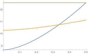
   Figure 3: The graphs of $2\alpha(c),2\pi+\beta(c)$ and $h(c)\equiv 4\pi$.

   From that $\beta(1/2)<2\pi$, it follows from the continuity with respect to $c$ and the fact that $c_{3}(S^{*}\mathcal{E}(1,1,1/2),\lambda)=4\pi$ that $c_{3}(S^{*}\mathcal{E}(1,1,c),\lambda)$ must coincide with $2\alpha(c)$ for all $c\in[1/3,1/2)$.

   Now let $1<c<c_{0}$. It follows from (37) that

   $$2\beta(c)=2w(c)=c_{3}(\operatorname{int}B^{4}(w(c),\omega_{0})\leq c_{3}(D^{*}\mathcal{E}(1,1,c),\omega_{can}).$$

   Hence, $c_{3}(D^{*}\mathcal{E}(1,1,c),\omega_{can})\geq 2\beta(c)>4\pi$. It is consequence of [10, Lemma 2.4] that $c_{3}(D^{*}\mathcal{E}(1,1,c),\omega_{can})$ is given by the total action of an actual Reeb orbit set for $(S^{*}\mathcal{E}(1,1,c),\lambda)$ and such a set must have trivial total homology class. Investigating all possible orbit sets, we shall conclude that the orbit set must consist in two meridians. Note that $2\beta(c)<2\beta(c_{0})=8\pi$ for $c<c_{0}$. Inspecting the toric domain $\mathbb{X}_{\Omega_{c}}$, one conclude that the orbits with action less than $8\pi$ are:

   • The two equators $\gamma_{1},\overline{\gamma}_{1}$ with action $2\pi$ each;

   • The meridians with action $\beta(c)$ provided $c<c_{0}$;

   • Nullhomologous orbits with action $a_{1}\in[4\pi,2\beta(c))$ which appears for any $c\geq 2$;

   • Orbits which are homologous to an equator traversed thrice and with action $a_{2}\geq 6\pi$ appearing for any $c\geq 3/2$ lying in the torus corresponding to the rational slope $2/3$.

   We recall that the equators and the meridians belongs to the nontrivial homology class in $H_{1}(S^{*}\mathcal{E}(1,1,c);{\mathbb{Z}})\cong{\mathbb{Z}}_{2}$. Thus, the possibilities of actions for nullhomologous orbit sets with action smaller than $8\pi$ are $4\pi,2\pi+2\beta(c),a_{1}$ and $2\beta(c)$. Further, we recall that $\beta(c)$ is simply the length of a meridian and then $\beta(1)=2\pi$. Putting together the continuity with respect to $c$, the fact $c_{3}(D^{*}\mathcal{E}(1,1,1),\omega_{can})=4\pi$ and the lower bound given by $2\beta(c)$, one can conclude that $c_{3}(D^{*}\mathcal{E}(1,1,c),\omega_{can})$ must be equal $\beta(c)$ until $c=c_{0}$, i.e., the parameter in which we have $2\beta(c)=8\pi$. This finishes the proof that $c_{3}(D^{*}\mathcal{E}(1,1,c)=2w(c)$ for $0<c<c_{0}$.

2. Let $c>1$. It is enough to prove that the orbit set $\alpha=\gamma_{1}\overline{\gamma}_{1}$ represents the generator $\zeta_{1}$ of $ECH_{2}^{<1/\varepsilon}(S^{*}\mathcal{E}(1,1,c),\lambda_{\varepsilon},0)$. This together with the fact that $\alpha$ is the nullhomologous orbit set with the possible least action yields $c_{1}(S^{*}\mathcal{E}(1,1,c),\lambda_{\varepsilon})=\mathcal{A}(\alpha)=4\pi$. For this, first we check that $\alpha$ has the correct degree:

   $$|\alpha| = \frac{1}{4}\left(sl({\gamma_{1}}^{2})+2lk({\gamma_{1}}^{2},{\overline{\gamma}_{1}}^{2})+sl({\overline{\gamma}_{1}}^{2})\right)+CZ_{\tau}(\gamma_{1})+CZ_{\tau}(\overline{\gamma}_{1})$$

   $$= \frac{1}{4}(-2+4-2)+1+1=2.$$

   Moreover, it follows from the properties that the ECH differential decreases action and decreases the grading by $1$ that $\alpha$ is closed, i.e., $\partial\alpha=0$. To see that $\alpha$ is not exact, suppose that there is a ECH chain complex generator $\beta$ such that $\langle\partial\beta,\alpha\rangle\neq 0$. In this case, there must exist an embedded pseudoholmoprhic curve $C$ in the symplectization of $S^{*}\mathcal{E}(1,1,c)$ with $p_{+}(C)$ positive punctures converging to $\beta$ and exactly $2$ negative punctures converging to $\alpha$ with Fredholm index given by

   $$\mathrm{ind}(C)=-\chi(C)+CZ_{\tau}^{\mathrm{ind}}(\beta)-CZ_{\tau}(\gamma_{1})-CZ_{\tau}(\overline{\gamma}_{1})=1.$$

   Thus,

   $$1=2g(C)+p_{+}(C)+CZ_{\tau}^{\mathrm{ind}}(\beta)-2,$$

   where $g(C)$ denotes the genus of the curve $C$. Since the Conley-Zehnder index of any orbit for our contact form is positive, we must have $g(C)=0$ and $p_{+}(C)=1$. Hence, $\beta$ consists in a single nullhomologous orbit, say $\widetilde{\gamma}$, with $CZ_{\tau}(\widetilde{\gamma})=2$. Further, $sl(\widetilde{\gamma})=1$ provided that

   $$3=|\beta|=sl(\widetilde{\gamma})+CZ_{\tau}(\widetilde{\gamma}).$$

   For $c>3/2$, there are indeed two Reeb orbits with Conley-Zehnder index $2$ and self-linking number $1$, namely the hyperbolic orbits arising from the two tori corresponding to the rational slope $2/3$. Both of these orbits belong to the homology class containing the equator, i.e., the nonzero class in $H_{1}(S^{*}\mathcal{E}(1,1,c);{\mathbb{Z}})\cong{\mathbb{Z}}_{2}$. In particular, a generator $\beta$ as above cannot exist and $\alpha$ is not exact.

∎

3.4 Symplectic embeddings and balls packings

We start this section recalling a version of Cristofaro-Gardiner’s result about the existence of symplectic embeddings from concave into (weakly) convex toric domains.

Let $\mathbb{X}_{\Omega}$ be a weakly convex toric domain. We construct a weight sequence as follows. For $b>0$, let $T(b)\subset{\mathbb{R}}^{2}$ denote the triangle with vertices $(0,0)$, $(b,0)$ and $(0,b)$. In particular $\mathbb{X}_{T(b)}=B^{4}(b)$. Let $w_{0}>0$ be the infimum of $w$ such that $\Omega\subset T(w)$. Let $\Omega_{1}$ and $\Omega_{2}$ be the closures of the components of $T(w_{0})\setminus\Omega$ containing $(w_{0},0)$ and $(0,w_{0})$, respectively. Then $\Omega_{1}$ and $\Omega_{2}$ are affinely equivalent to the moment map image of concave toric domains. In fact, after translating $\Omega_{1}$ by $(-b,0)$ and multiplying it by $\begin{pmatrix}0&1\\ -1&-1\end{pmatrix}$ we obtain a region $\Omega_{1}^{\prime}\subset{\mathbb{R}}^{2}$ such that $\mathbb{X}_{\Omega_{1}}$ is a concave toric domain. We can proceed analogously with $\Omega_{2}$ to obtain $\Omega_{2}^{\prime}$. Now we let $w_{1}$ be the supremum of $w$ such that $T(w)\subset\Omega_{1}^{\prime}$. We define $w_{2}$ analogously for $\Omega_{2}^{\prime}$. The sets $\Omega_{1}^{\prime}\setminus T(w_{1})$ and $\Omega_{2}^{\prime}\setminus T(w_{1})$ each have at most two connected components, all of whose closures are affinely equivalent to moment map images of concave toric domains. Inductively, we obtain a sequence of numbers

$$(w_{0};w_{1},w_{2},\dots),$$

which is called the weight sequence of $\mathbb{X}_{\Omega}$.

Theorem 3.3 (Cristofaro-Gardiner [5]).

Let $\mathbb{X}_{\Omega}$ be a weakly convex toric domain and let $(w_{0};w_{1},w_{2},\dots)$ be its weight sequence. Then $B^{4}(a)\hookrightarrow\mathbb{X}_{\Omega}$ if, and only if

$$B^{4}(a)\sqcup\bigsqcup_{i=1}^{\infty}B^{4}(w_{i})\hookrightarrow B^{4}(w_{0}).$$

We can now prove Proposition 1.8 for $c>1$.

Proof of Proposition 1.8 for $c>1$.

First assume that $1\leq c\leq c_{0}$, which implies that $w(c)=\beta(c)\leq 4\pi$. From Proposition 2.7 we know that the toric domain $\mathbb{X}_{\Omega_{c}}$ is weakly convex. Since $\Omega_{c}$ is symmetric by reflections about the line $x=y$, it follows that $w_{0}=2t$, where $(t,t)$ is the intersection of the curve (22) with the line $x=y$. So $w_{0}=2g_{c}(0)=2\beta(c)$. Since the curve (22) has vertical and horizontal tangents at the point $(\beta(c),\beta(c))$, by the proof of Proposition 29, it follows that $w_{1}=w_{2}=\beta(c)$. The slope of the tangent line to the curve (22) at $(2\pi,0)$ is

$$\frac{g_{c}^{\prime}(j)}{g_{c}^{\prime}(j)+2\pi}=\frac{-2\pi c}{-2\pi c+2\pi}=\frac{c}{c-1}>1.$$

So $w_{3}=\beta(c)-2\pi$. We now construct a ball packing

$$B^{4}(\beta(c))\sqcup\bigsqcup_{i=1}^{\infty}B^{4}(w_{i})\hookrightarrow B^{4}(w_{0}).$$

We start by leaving all of the triangles coming from $\Omega_{2}$ where they are found. We also leave the triangle $T(\beta(c))$ corresponding to $w_{1}$ in its original place in $\Omega_{1}$. Now we take $T(w_{3})$ to the triangle with vertices $(4\pi-\beta(c),2\pi)$, $(2\pi,2\pi)$ and $(\beta(c),\beta(c))$. The remaining triangles in $\Omega_{1}$ fit into the triangle with vertices $(2\pi,0)$, $(\beta(c),2\pi)$ and $(\beta(c),\beta(c))$, which is affinely equivalent to the triangle with vertices $(0,0)$, $(0,2\pi)$ and $(\beta(c)-2\pi,2\pi)$. So we set them in the latter triangle. Finally we can place $T(\beta(c))$ in the triangle with vertices $(0,0)$, $(\beta(c),0)$ and $(\beta(c),\beta(c))$, yielding the desired ball packing, see Figure 4. It follows from Theorem 3.3 that

$$B^{4}(\beta(c))\hookrightarrow\mathbb{X}_{\Omega_{c}}.$$ (39)

(a) The weight sequence of $\Omega_{c}$

(b) The ball packing into $B^{4}(w_{0})$

Figure 4: The construction of the ball packing

Now suppose that $c>c_{0}$. Then $w(c)=4\pi=\beta(c_{0})$. Moreover, recall from (25) that $g_{c}(j)$ can be written as

$$g_{c}(j)=4\int_{0}^{c\sqrt{1-j^{2}}}\frac{\sqrt{(c^{2}(1-j^{2})-z^{2})(c^{4}+(1-c^{2})z^{2})}}{c(c^{2}-z^{2})}\,dz$$

and making the substitution $r=\sqrt{\frac{c-z}{c+z}}$ yields

$$g_{c}(j)=4\int_{0}^{\frac{1-\sqrt{1-j^{2}}}{\sqrt{2-j^{2}}}}\sqrt{\left(\frac{4}{(1+r^{2})^{2}}-\frac{j^{2}}{r^{2}}\right)\frac{r^{4}+(4c^{2}-2)r^{2}+1}{(1+r^{2})^{2}}}dr.$$

In particular, $g_{c}(j)$ is increasing wit respect to $c$. So $\mathbb{X}_{\Omega_{c_{0}}}\subset\mathbb{X}_{\Omega_{c}}$. Using (39) for $c_{0}$ we conclude that

$$B^{4}(w(c))=B^{4}(\beta(c_{0}))\hookrightarrow\mathbb{X}_{\Omega_{c_{0}}}\subset\mathbb{X}_{\Omega_{c}}.$$

∎

Instituto de Matemática Pura e Aplicada, Rio de Janeiro, Brazil

E-mails: brayan.ferreira@impa.br, vgbramos@impa.br, kvicente@impa.br

References

- [1] Abbondandolo, A., Bramham, B., Hryniewicz, U. L., and Salomão, P. A. A systolic inequality for geodesic flows on the two-sphere. Mathematische Annalen 367, 1 (2017), 701–753.
- [2] Arnol’d, V. I. Mathematical methods of classical mechanics, vol. 60. Springer Science & Business Media, 2013.
- [3] Choi, K., Cristofaro-Gardiner, D., Frenkel, D., Hutchings, M., and Ramos, V. G. B. Symplectic embeddings into four-dimensional concave toric domains. Journal of Topology 7, 4 (2014), 1054–1076.
- [4] Cieliebak, K., and Latschev, J. The role of string topology in symplectic field theory. New perspectives and challenges in symplectic field theory 49 (2009), 113–146.
- [5] Cristofaro-Gardiner, D. Symplectic embeddings from concave toric domains into convex ones. Journal of Differential Geometry (2019).
- [6] Eliasson, L. Hamiltonian systems with poisson commuting integrals. PhD thesis, University of Stockholm (1984).
- [7] Eliasson, L. Normal forms for hamiltonian systems with poisson commuting integrals—elliptic case. Commentarii Mathematici Helvetici 65, 1 (1990), 4–35.
- [8] Ferreira, B., and Ramos, V. G. B. Symplectic embeddings into disk cotangent bundles. Journal of Fixed Point Theory and Applications 24, 3 (2022), 1–31.
- [9] Hutchings, M. Lecture notes on embedded contact homology. In Contact and symplectic topology. Springer, 2014, pp. 389–484.
- [10] Irie, K. Dense existence of periodic reeb orbits and ech spectral invariants. Journal of Modern Dynamics 9, 01 (2015), 357.
- [11] Klingenberg, W. Riemannian Geometry, vol. 1. Walter de Gruyter, 1995.
- [12] Ostrover, Y., and Ramos, V. G. Symplectic embeddings of the lp-sum of two discs. Journal of Topology and Analysis (2021), 1–29.
- [13] Ramos, V. G. B. Symplectic embeddings and the lagrangian bidisk. Duke Mathematical Journal 166 (2017), 1703–1738.
- [14] Taubes, C. H. Embedded contact homology and Seiberg–Witten Floer cohomology I. Geometry & Topology 14, 5 (2010), 2497–2581.
- [15] Traynor, L. Symplectic packing constructions. Journal of Differential Geometry 41, 3 (1995), 735–751.
- [16] Zelditch, S. The inverse spectral problem for surfaces of revolution. Journal of Differential Geometry 49, 2 (1998), 207–264.