Semi-analytical computation of heteroclinic connections between center manifolds with the parameterization method

Abstract

This paper presents methodology for the computation of whole sets of heteroclinic connections between iso-energetic slices of center manifolds of center  $\times$  center  $\times$  saddle fixed points of autonomous Hamiltonian systems. It involves: (a) computing Taylor expansions of the center-unstable and center-stable manifolds of the departing and arriving fixed points through the parameterization method, using a new style that uncouples the center part from the hyperbolic one, thus making the fibered structure of the manifolds explicit; (b) uniformly meshing iso-energetic slices of the center manifolds, using a novel strategy that avoids numerical integration of the reduced differential equations and makes an explicit 3D representation of these slices as deformed solid ellipsoids; (c) matching the center-stable and center-unstable manifolds of the departing and arriving points in a Poincaré section. The methodology is applied to obtain the whole set of iso-energetic heteroclinic connections from the center manifold of $L_{2}$ to the center manifold of $L_{1}$ in the Earth-Moon circular, spatial Restricted Three-Body Problem, for nine increasing energy levels that reach the appearance of Halo orbits in both $L_{1}$ and $L_{2}$. Some comments are made on possible applications to space mission design.

Keywords. Parameterization method; Heteroclinic connections; Invariant tori; Libration point orbits; RTBP; Center manifolds.

1 Introduction

Heteroclinic connections play an important role in the description of dynamical systems from a global point of view. In this work we address the systematic computation of heteroclinic connections between center manifolds of fixed points of center$\times$center$\times$saddle type of autonomous, 3-degrees-of-freedom Hamiltonian systems.

Our interest in this case comes from applications in Astrodynamics, namely to Libration Point (LP) space missions. In these missions, spacecraft are sent to orbits that stay close to the fixed (in a rotating frame) points $L_{1}$, $L_{2}$ of the spatial, circular restricted three-body problem (RTBP). This model describes the dynamics of a massless particle under the attraction of two celestial bodies, called primaries, that revolve in circles around their common center of mass. Examples of primaries are the Sun and a planet, or a planet and a moon. Among the advantages of these missions are the absence of the shadow of a celestial body, thus providing a more stable thermal environment, and continuous access to the whole celestial sphere, except for a direction, that is not fixed but rotates with the primaries. An actual example of the use of these advantages is found in the orbit of the James Webb Space Telescope, around Sun-Earth $L_{2}$, when compared to the orbit of the Hubble Space Telescope, around Earth. See [10] for a survey of early LP missions, and the webs of the space agencies for many newer ones.

From the point of view of the dynamics of the RTBP [15, 16, 12, 13], orbits in the center manifold of the $L_{1},L_{2}$ points provide nominal orbits for LP missions, whereas their invariant stable and unstable manifolds provide transfer orbits either from Earth to a nominal orbit or between nominal orbits. Focusing in this last case, missions that have used trajectories close to heteroclinic connections are Genesis [22] and Artemis [35]. The main motivation of this paper is to contribute towards the systematic design of similar missions.

For the Sun–Jupiter planar RTBP, a heteroclinic connection between an object of the center manifold of $L_{1}$ and an object of the center manifold of $L_{2}$, namely a planar Lyapunov periodic orbit (p.o.) in each case, is used in the celebrated paper [24] in order to explain the (apparently) erratic behavior of the comet Oterma. This heteroclinic connection is part of one of the many families of connections between Lyapunov p.o. explored in [7]. Some connections between Lyapunov p.o. have also been proven to exist through rigorous numerics [37, 38]. The first work that addresses the systematic computation of heteroclinic connections between center manifolds of libration points, thus also obtaining connections between invariant tori, is [18]. The computations of this reference are used in [14] in order to extend the results of [24] to the spatial RTBP. Reference [1] is the first and only work (as far as we know) that computes the whole set of heteroclinic connections between the center manifolds of $L_{1}$ and $L_{2}$ for a fixed energy level. It does so not for the spatial RTBP but for the spatial Hill’s problem. The methodology used is a combination of the Lindstedt-Poincaré expansions introduced in [26] with the modification of the reduction to the center manifold technique [12, 23] used in [18]. The set of connections found in [1] is shown in [9] to define a scattering map.

In this paper we introduce a new technique for the computation of whole sets of heteroclinic connections between iso-energetic slices of the center manifolds of $L_{1}$ and $L_{2}$, that is applicable to center$\times$center$\times$saddle fixed points of any 3-degrees-of-freedom, autonomous Hamiltonian system. Compared to the one of [1], ours is a procedure that provides less insight on the fine structure of the set of connections, but on the other hand it is more automatic and simpler to carry out, and thus more adequate for the systematic exploration of phase space. Our procedure relies solely on the semi-analytical computation of center-unstable and center-stable manifolds. By avoiding the use of Lindstedt-Poincaré expansions, it is also able to reach larger levels of energy.

The center-unstable and center-stable manifolds of $L_{1}$, $L_{2}$ are computed through the parameterization method. The parameterization method, first introduced in [4, 5, 6], has proven to be a valuable tool in both the theoretical proof of existence of invariant manifolds and their computation, due to the fact that the proofs are constructive and can be turned into algorithms. Our approach is purely computational, and our starting point is chapter 2 of [20]. To the parameterization styles described there, we add a mixed-uncoupling style that, besides adapting the parameterization to the dynamics by making certain sub-manifolds invariant, it is able to decouple the hyperbolic part from the central one, thus making the fibered structure of the manifolds explicit. The implementation of this new style of parameterization has been done starting from the software from chapter 2 of [20], which is available at http://www.maia.ub.es/dsg/param/.

A key point for our procedure to be systematic and to require little human intervention is being able to produce equally-spaced meshes of iso-energetic slices of the center manifold in a computationally efficient manner. Classically, the center manifold of the collinear points of the spatial, circular RTBP has been described globally through iso-energetic Poincaré sections, that are two-dimensional and thus easily visualized [12, 23, 17]. A first strategy would be to globalize these Poincaré sections to the iso-energetic slice through numerical integration of the reduced equations. This turns out to be very expensive because the reduced equations are given by high-order expansions of 4-variate functions. The strategy we propose here avoids numerical integration completely, and also makes explicit the representation of a 3D projection of the iso-energetic slice as a deformed solid ellipsoid, that is what we actually mesh. On the topological structure of iso-energetic slices of the center manifold, see e.g. [8, 27, 28, 14].

The proposed methodology is applied in order to obtain the whole set of heteroclinic connections from the center manifold of $L_{2}$ to the center manifold of $L_{1}$ of the Earth-Moon spatial, circular RTBP for 3 groups of 3 energy levels, each group of connections performing a different number of revolutions around the Moon. For the last group of energies, the Halo family of p.o. has already appeared, meaning that these energies are relatively far from the equilibrium point. We have chosen Earth and Moon as primaries because of its intrinsic interest in space flight, and also in order to see that the methodology works in a case in which, at fixed energies, the dynamics around $L_{1}$ and $L_{2}$ are highly asymmetric one with respect to the other.

The paper is structured as follows: Section 2 introduces the spatial, circular RTBP and provides several data related to the linear dynamics around $L_{1}$, $L_{2}$. Section 3 summarizes the parameterization method for invariant manifolds of fixed points of flows, and introduces our mixed-uncoupling style of parameterization for the computation of center-stable and center-unstable manifolds. Section 4 introduces our meshing strategy for iso-energetic slices of the center manifold. For the restrictions of the center-unstable manifold of $L_{2}$ and the center-stable one of $L_{1}$ to the corresponding center manifolds, several meshes are computed and used to test the validity of the expansions and decide the order to be used and the energy range to be explored. Section 5 describes the strategy we follow to obtain the whole set of heteoclinic connections of an energy level from meshes of the center manifolds of $L_{2}$ and $L_{1}$. Finally, in Section 6, the whole set of heteroclinic connections is computed for the 9 energy levels mentioned previously.

2 The spatial, circular RTBP

In this section we recall some facts about the spatial, circular Restricted Three-Body Problem (RTBP) that will be used in the following sections. For more details, see e.g. [36].

The spatial, circular RTBP describes the motion of a particle of infinitesimal mass which is considered to be under the gravitational influence of two other massive bodies, known as primaries, that move in circular orbits around their center of masses. Let us denote by $m_{1}$ and $m_{2}$ the masses of the primaries, chosen in order to have $m_{1}>m_{2}$. By taking as origin the center of mass and considering a uniformly rotating coordinate system with the same period as the primaries, called synodic, the primaries can be made to remain fixed in the horizontal axis. By further taking dimensionless distance and time units as to have the distance between the primaries equal to $1$ and their period of rotation equal to $2\pi$, the differential equations depend on a single parameter $\mu=m_{2}/(m_{1}+m_{2})\in[0,1/2)$. By finally introducing momenta as $p_{x}=\dot{x}-y$, $p_{y}=\dot{y}+x$ and $p_{z}=\dot{z}$, the behavior of the particle of infinitesimal mass is described by the following set of differential equations,

$$\dot{x} =p_{x}+y,\quad \dot{p}_{x} =p_{y}-\frac{1-\mu}{r_{1}^{3}}(x-\mu)-\frac{\mu}{r_{2}^{3}}(x-\mu+1),$$ (1)

$$\dot{y} =p_{y}-x,\quad \dot{p}_{y} =-p_{x}-\frac{1-\mu}{r_{1}^{3}}y-\frac{\mu}{r_{2}^{3}}y,$$

$$\dot{z} =p_{z},\quad \dot{p}_{z} =-\frac{1-\mu}{r_{1}^{3}}z-\frac{\mu}{r_{2}^{3}}z,$$

with $r_{1}$ and $r_{2}$ defined as

$$r_{1}=\sqrt{(x-\mu)^{2}+y^{2}+z^{2}},\qquad r_{2}=\sqrt{(x-\mu+1)^{2}+y^{2}+z^{2}}.$$

This set of differential equations is a Hamiltonian system with associated Hamiltonian

$$H(x,y,z,p_{x},p_{y},p_{z})=\frac{1}{2}(p_{x}^{2}+p_{y}^{2}+p_{z}^{2})-xp_{y}+yp_{x}-\frac{1-\mu}{r_{1}}-\frac{\mu}{r_{2}}.$$ (2)

Due to symmetries in the differential equations (1), if $\bigl{(}x(t),y(t),z(t),p_{x}(t),p_{y}(t),p_{z}(t)\bigr{)}$ is a solution, then

$$\bigl{(}x(-t),-y(-t),z(-t),-p_{x}(-t),p_{y}(-t),-p_{z}(-t)\bigr{)}$$ (3)

and

$$\bigl{(}x(t),y(t),-z(t),p_{x}(t),p_{y}(t),-p_{z}(t)\bigr{)}$$

are also solutions.

It is well known that the RTBP has five equilibrium points. Two of them, called Lagrangian and denoted by $L_{4},L_{5}$, form equilateral triangles with the primaries. The remaining three, called collinear and denoted by $L_{1},L_{2},L_{3}$, lie on the line joining the primaries, this is, the $x$ axis, see Figure 1. Their distances to the closest primary are given by the only positive root of the corresponding Euler’s quintic equation

$$\gamma_{j}^{5}\mp(3-\mu)\gamma_{j}^{4}+(3-2\mu)\gamma_{j}^{3}-\mu\gamma_{j}^{2}\pm 2\mu\gamma_{j}-\mu =0,\quad j =1,2,$$

$$\gamma_{j}^{5}+(2+\mu)\gamma_{j}^{4}+(1+2\mu)\gamma_{j}^{3}-(1-\mu)\gamma_{j}^{2}-2(1-\mu)\gamma_{j}-(1-\mu) =0,\quad j =3,$$

so that, if we denote the $x$ coordinate of the $L_{j}$ point as $x_{L_{j}}$, we have $x_{L_{1}}=\mu-1+\gamma_{1}$, $x_{L_{2}}=\mu-1-\gamma_{2}$, $x_{L_{3}}=\mu+\gamma_{3}$.

An important property of the collinear equilibrium points is that their associated set of eigenvalues has the following form

$$\mathop{\rm Spec}\nolimits DF(L_{j})=\{{\bm{i}}\omega_{1}^{(j)},-{\bm{i}}\omega_{1}^{(j)},{\bm{i}}\omega_{2}^{(j)},-{\bm{i}}\omega_{2}^{(j)},\lambda^{(j)},-\lambda^{(j)}\},\quad j=1,2,3,$$

where ${\bm{i}}$ denotes the imaginary unit, so their linear behaviour is center$\times$center$\times$saddle. For this set of eigenvalues, the corresponding eigenvectors will be denoted as

$$\begin{matrix}u^{(j)},&\bar{u}^{(j)},&v^{(j)},&\bar{v}^{(j)},&w_{+}^{(j)},&w_{-}^{(j)},\\ \end{matrix}$$

where the overline denotes complex conjugation and

$$u^{(j)}=u_{r}^{(j)}-{\bm{i}}u_{i}^{(j)},\quad v^{(j)}=v_{r}^{(j)}-{\bm{i}}v_{i}^{(j)}.$$ (4)

Figure 1: For the Earth-Moon mass parameter, scheme of the RTBP equilibrium points.

From now on, $\mu$ will be the Earth-Moon mass ratio, taken as

$$\mu=1.215058560962404\cdot 10^{-2},$$

as obtained from the DE406 JPL ephemeris file [34].

The eigenvalues in each one of the two equilibrium points under study are numerically found to be

$$\omega_{1}^{(1)} =2.334385885086,\quad \omega_{2}^{(1)} =2.268831094972,\quad \lambda^{(1)} =2.93205593364,$$

$$\omega_{1}^{(2)} =1.862645862176513,\quad \omega_{2}^{(2)} =1.78617614289,\quad \lambda^{(2)} =2.1586743203.$$

Note that, since neither $\omega_{1}^{(j)}$ is an integer multiple of $\omega_{2}^{(j)}$ nor $\omega_{2}^{(j)}$ is an integer multiple of $\omega_{1}^{(j)}$, Lyapunov’s center theorem [33, 28] applies to each pair of complex eigenvalues, so two families of p.o. are born from each collinear equilibrium point. Each one of these families spans a 2-dimensional manifold which is tangent to the real and imaginary part of the eigenvectors associated to each $\pm{\bm{i}}\omega_{i}$ eigenvalue at the equilibrium point. The planar (resp. vertical) family is tangent to eigenvectors with zero $z,p_{z}$ (resp. $x,y,p_{x},p_{y}$) components. From now on, the planar (resp. vertical) eigenvalues will be denoted as $\pm{\bm{i}}\omega_{p}$ (resp. $\pm{\bm{i}}\omega_{v}$), in order to emphasize their direction. According to the numerical values given above, $\omega_{p}^{(j)}=\omega_{1}^{(j)}$ and $\omega_{v}^{(j)}=\omega_{2}^{(j)}$.

3 Parameterizing center-stable and center-unstable manifolds

For the purpose of computing all the possible heteroclinic connections from the center manifold of $L_{2}$ to the one of $L_{1}$, to be denoted as ${\mathcal{W}}^{c}(L_{2})$, ${\mathcal{W}}^{c}(L_{1})$ from now on, parameterizations of the center-unstable manifold of $L_{2}$ and center-stable manifold of $L_{1}$ are needed. The center-unstable manifold of $L_{2}$ (resp. center-stable manifold of $L_{1}$) will be denoted as ${\mathcal{W}}^{cu}(L_{2})$ (resp. ${\mathcal{W}}^{cs}(L_{1})$) from now on. Parameterizations of these manifolds are found by means of the parameterization method of invariant manifolds of fixed points of flows (PMFPF) as presented in chapter 2 of [20]. To the development of [20], we add a mixed-uncoupling style, that effectively uncouples the central and hyperbolic part in such a way that, for any point in a center-stable or center-unstable manifold, the point of the center manifold at the base of the corresponding fiber is obtained by setting to zero the last parameter. In this section, we first recall the PMFPF briefly. After that, we introduce our mixed-uncoupled style and discuss its application to the computation of ${\mathcal{W}}^{cu}(L_{2})$ and ${\mathcal{W}}^{cs}(L_{1})$. We end the section with some comments on how this mixed-uncoupled style makes the fibered structure of the manifolds explicit.

Consider a $n$-dimensional dynamical system

$$\dot{Z}=F(Z),$$ (5)

whose flow is $\Phi_{t}$ and has a fixed point $Z_{0}$, this is $F(Z_{0})=0$. We assume for simplicity that $DF(Z_{0})$ has $n$ distinct eigenvalues $\lambda_{1},\dots,\lambda_{n}$, with corresponding eigenvectors $v_{1},\dots,v_{n}$, this is

$$DF(Z_{0})v_{j}=\lambda_{j}v_{j},\quad j=1,\dots,n,$$

with $\lambda_{j}\in\mathbb{C}$, $v_{j}\in\mathbb{C}^{n}$. Our purpose consists in computing a $d$-dimensional manifold containing $Z_{0}$ and tangent to the linear space spanned by some of its eigenvectors.

For that, we consider the change of variables given by $Z=Z_{0}+Pz$, so that the new system of ODE $\dot{z}=G(z)$ has the origin as a fixed point, and the differential of the vector field evaluated at the new fixed point is diagonal with $DG(0)=\text{diag}\{\lambda_{1},\dots,\lambda_{n}\}$. Note that $P$ is a matrix composed by the eigenvectors in such a way that the first $d$ components correspond to those eigendirections that we want our parameterization to be tangent to.

Then, our problem turns into computing an expansion of a $d$-dimensional manifold containing the origin, invariant by the flow described by $G$ and tangent to the first $d$ components of $z$ at $z=0$. Then, let us denote by $W:\mathbb{C}^{d}\to\mathbb{C}^{n}$ the parameterization of the manifold and by $f:\mathbb{C}^{d}\to\mathbb{C}^{d}$ the reduced vector field, so that, if the manifold is parameterized as $W(s)$, the differential equations reduced to the manifold are $\dot{s}=f(s)$. For this to be true, the following invariance equation must be satisfied,

$$\psi_{t}\bigl{(}W(s)\bigr{)}=W\bigl{(}\phi_{t}(s)\bigr{)},$$

where $\psi_{t}$ and $\phi_{t}$ are the flows of $\dot{z}=G(z)$ and $\dot{s}=f(s)$, respectively. By differentiating with respect to $t$ and taking $t=0$, the infinitesimal version of the invariance equation is obtained,

$$G(W(s))=DW(s)f(s),$$ (6)

which is the equation that we actually solve for $W,f$.

The way of solving this invariance equation (6) consists on computing power series expansions for both $W$ and $f$. Denote $W(s)=\bigl{(}W^{1}(s),\dots,W^{n}(s)\bigr{)}$, $f(s)=\bigl{(}f^{1}(s),\dots,f^{d}(s)\bigr{)}$ and

$$W^{i}(s)=\sum_{k\geq 0}W^{i}_{k}(s),\quad f^{i}(s)=\sum_{k\geq 0}f^{i}_{k}(s),$$

where $W^{i}_{k}(s)=\sum_{|m|=k}W_{m}^{i}s^{m}$, $f_{k}^{i}(s)=\sum_{|m|=k}f_{m}^{i}s^{m}$, $m=(m_{1},\dots,m_{d})\in\mathbb{N}^{d}$, $|m|=m_{1}+\dots+m_{d}$, $s=(s_{1},\dots,s_{d})$ and $s^{m}=s_{1}^{m_{1}}\dots s_{d}^{m_{d}}$. Using these expansions, equation (6) is solved order by order. Orders 0 and 1 are obtained as

$$f_{0}(s) =(0,\dots,0),\quad W_{0}(s) =(0,\dots,0),$$ (7)

$$f_{1}(s) =(\lambda_{1}s_{1},\dots,\lambda_{d}s_{d}),\quad W_{1}(s) =(s_{1},\dots,s_{d},0,\dots,0).$$

Imposing (6) at order $k$ leads to the $k$-th order cohomological equation, whose right-hand side is given by all the known terms up to order $k-1$,

$$R(s)=[G(W_{<k}(s))]_{k}-\sum_{l=2}^{k-1}DW_{k-l+1}(s)f_{l}(s),$$

where $W_{<k}(s)$ is the power series expansion of the manifold up to order $k-1$ and $[\cdot]_{k}$ denotes “terms of order $k$”. In terms of this $R$, the cohomological equation becomes, at the coefficient level,

$$(\langle\lambda,m\rangle-\lambda_{i})W_{m}^{i}+f_{m}^{i} =R_{m}^{i},\quad i\in\{1,\dots,d\}$$ (8)

$$(\langle{\lambda},m\rangle-\lambda_{i})W_{m}^{i} =R_{m}^{i},\quad i\in\{d+1,\dots,n\}.$$

Here we assume $R=(R^{1},\dots,R^{n})$, $R^{i}(s)=\sum_{|m|=k}R^{i}_{m}s^{m}$, and $\lambda=(\lambda_{1},\dots,\lambda_{d})$, so that $\langle{\lambda},m\rangle=\lambda_{1}m_{1}+\dots+\lambda_{d}m_{d}$.

The first line of (8) is known as the tangent part, while the second line is called the normal part. For (8) to have solution, it is necessary that its normal part has no cross resonances, this is, $\langle{\lambda},m\rangle\neq\lambda_{i}$ for all $m\in\mathbb{N}^{d}$ and $i\in\{d+1,\dots,n\}$. In order to solve the tangent part, we can either (a) take $W^{i}_{m}=0$ and $f^{i}_{m}=R^{i}_{m}$ or (b) take $f^{i}_{m}=0$ and $W^{i}_{m}=R^{i}_{m}/(\langle{\lambda},m\rangle-\lambda_{i})$. For this last choice to be possible, $(i,m)$ cannot be an inner resonance, this is, $\langle{\lambda},m\rangle\neq\lambda_{i}$. A style of parameterization is a rule that determines the choice between (a) and (b) as a function of $(i,m)$. Some styles of parameterization are discussed in [20].

For our purposes, it will be convenient to introduce a mixed-uncoupling style, in which we require that several sub-manifolds of the form $\{s_{i_{1}}=s_{i_{2}}=\dots=s_{i_{J}}=0\}$ are invariant, and we also require that the first $d-1$ equations of the reduced system of equations are uncoupled from the last one. For a general $(i,m)$, in order to keep the parameterization simple, we will want to choose (a) above unless it is incompatible with the invariance and uncoupling requirements. For the invariance requirement we follow [20]: if $I_{1},\dots,I_{N}\subset\{1,\dots,d\}$ are such that $\{s_{i}=0,i\in I_{j}\}$, $j=1,\dots,N$ are required to be invariant, we choose (b) if $\exists j:i\in I_{j}$ and $m_{l}=0$ $\forall l\in I_{j}$. For the uncoupling requirement, we need to eliminate the dependence of $f^{1},\dots,f^{d-1}$ on $s_{d}$. In order to achieve this, we choose (b) if $1\leq i\leq d-1$ and $m_{d}\neq 0$. For both the sub-manifold invariance and uncoupling requirements, it is necessary that $(i,m)$ is not an internal resonance when choosing (b).

In our case, we want to compute ${\mathcal{W}}^{cu}(L_{2})$ and ${\mathcal{W}}^{cs}(L_{1})$ for the Earth-Moon circular, spatial RTBP (see Section 2). The choices for the ordering of eigenvalues are

$$\lambda_{1,2}=\pm{\bm{i}}\omega_{p}^{(2)},\ \lambda_{3,4}=\pm{\bm{i}}\omega_{v}^{(2)},\ \lambda_{5}>0$$ (9)

for ${\mathcal{W}}^{cu}(L_{2})$, and

$$\lambda_{1,2}=\pm{\bm{i}}\omega_{p}^{(1)},\ \lambda_{3,4}=\pm{\bm{i}}\omega_{v}^{(1)},\ \lambda_{5}<0$$ (10)

for ${\mathcal{W}}^{cs}(L_{1})$. We use the mixed-uncoupling style just described with $d=5$, $N=3$, $I_{1}=\{5\}$, $I_{2}=\{3,4\}$, $I_{3}=\{1,2\}$. This is, in addition to uncoupling the first $4$ equations from the $5$-th one, we want the submanifolds $\{s_{5}=0\}$, $\{s_{3}=s_{4}=0\}$ and $\{s_{1}=s_{2}=0\}$ to be invariant. There are no internal resonances in all the choices involved, namely:

1. For the uncoupling, we need $\langle\lambda,m\rangle-\lambda_{i}\neq 0$ if $m_{5}\neq 0$ and $i=1,\dots,4$. This is true because $\mathop{\rm Re}\nolimits\langle\lambda,m\rangle\neq 0$, since $\mathop{\rm Re}\nolimits(\lambda_{d}m_{d})\neq 0$ and $\mathop{\rm Re}\nolimits(\lambda_{1}m_{1}+\dots+\lambda_{4}m_{4})=0$.

2. For $\{s_{5}=0\}$ to be invariant, we need that $\lambda_{5}\neq\langle\lambda,m\rangle$ if $m_{5}=0$. This is necessarily true since $\mathop{\rm Re}\nolimits(\lambda_{1}m_{1}+\dots+\lambda_{4}m_{4})=0$.

3. For $\{s_{1}=s_{2}=0\}$ to be invariant, we need that $\lambda_{1,2}\neq\langle\lambda,m\rangle$ if $m_{1}=m_{2}=0$. If $m_{5}\neq 0$, it is true by the argument in (a). If $m_{5}=m_{1}=m_{2}=0$, to have $\lambda_{1}=\langle\lambda,m\rangle$ or $\lambda_{2}=\langle\lambda,m\rangle$ would imply that $\omega_{p}^{(j)}$ is an integer multiple of $\omega_{v}^{(j)}$ which it is not true, by the hypothesis of Lyapunov’s center theorem for the existence of the vertical Lyapunov family (see Section 2).

4. For $\{s_{3}=s_{4}=0\}$, an analogous argument can be made.

Following the notations of Section 2, the RTBP equations (1) are first diagonalized by choosing

$$P =\begin{bmatrix}u^{(2)}&\bar{u}^{(2)}&v^{(2)}&\bar{v}^{(2)}&w_{+}^{(2)}&w_{-}^{(2)}\end{bmatrix},\quad\mbox{for ${\mathcal{W}}^{cu}(L_{2})$},$$ (11)

$$P =\begin{bmatrix}u^{(1)}&\bar{u}^{(1)}&v^{(1)}&\bar{v}^{(1)}&w_{-}^{(1)}&w_{+}^{(1)}\end{bmatrix},\quad\mbox{for ${\mathcal{W}}^{cs}(L_{1})$}.$$

These choices lead to complex systems of ODE $\dot{z}=G(z)$, and therefore to complex parameterizations. Following [20], the original real center-unstable and center-stable manifolds are obtained, for real $s$, as

$$\tilde{W}(s)=Z_{0}+PW(Cs),$$ (12)

where $C$ is the $d\times d$ block-diagonal, square matrix

$$C=\begin{pmatrix}1&{\bm{i}}&0&0&0\\ 1&-{\bm{i}}&0&0&0\\ 0&0&1&{\bm{i}}&0\\ 0&0&1&-{\bm{i}}&0\\ 0&0&0&0&1\\ \end{pmatrix}.$$ (13)

The ordering of eigenvalues in (9) (resp. (10)) implies that $\{s_{5}=0\}$ describes ${\mathcal{W}}^{c}(L_{2})$ (resp. ${\mathcal{W}}^{c}(L_{1})$), $\{s_{3}=s_{4}=0\}$ describes the unstable (resp. stable) manifold of the planar Lyapunov family of periodic orbits, and $\{s_{1}=s_{2}=0\}$ describes the unstable (resp. stable) manifold of the vertical Lyapunov family of periodic orbits. By an intersection argument, $\{s_{3}=s_{4}=s_{5}=0\}$ describes the planar Lyapunov family of p.o. and $\{s_{1}=s_{2}=s_{5}=0\}$ describes the vertical Lyapunov family of p.o.

Thanks to conditions (a) and (b) above, parameter space can be considered a fibered space in which the base of each fiber is described by the coordinates $s_{1},\dots,s_{4}$, and $s_{5}$ is the coordinate on each fiber. The reduced flow sends fibers to fibers, since

$$\phi_{t}^{i}(s_{1},\dots,s_{4},s_{5}^{(1)})=\phi_{t}^{i}(s_{1},\dots,s_{4},s_{5}^{(2)}),\quad i=1,\dots,4,$$

for all $s_{1},\dots,s_{4},s_{5}^{(1)},s_{5}^{(2)}$. Recall that we are computing center stable (resp. unstable) manifolds so any initial condition in the manifold will tend to the center manifold forward (resp. backward) in time. Since the center manifold is described by $s_{5}=0$, this means that the last component of the reduced flow will also tend to 0. As a consequence, for $\tilde{W}(s_{1},\dots,s_{4},0)$ in any object of the center manifold (fixed point, periodic orbit, invariant torus, etc.), the corresponding fiber in the stable (resp. unstable) manifold of the object is given by $\tilde{W}(s_{1},\dots,s_{4},s_{5})$ for $s_{5}\neq 0$. Of course, $|s_{5}|$ has to be small enough for the expansions to be accurate.

4 Meshing iso-energetic slices of the center manifold

In this section, we present an strategy to obtain equally-spaced meshes of iso-energetic slices of center manifolds of center$\times$center$\times$saddle fixed points of 3-degrees-of-freedom, autonomous Hamiltonian systems. A first approach to deal with this problem would consist in globalizing by means of numerical integration the classical representation of the center manifold as a sequence of iso-energetic Poincaré sections [12, 23, 17]. However, this procedure involves the evaluation of the expansions obtained from the PMFPF, which is expensive in terms of computational time. Instead of that, a geometrical approach is taken in which, by considering the quadratic part of the Hamiltonian applied to the parameterization, the iso-energetic slice is described in terms of a deformed solid ellipsoid. The strategy is used to perform an exploration in order to determine the order and energy ranges to be used in the computations of the following sections.

Consider parameterizations $\tilde{W}^{(1)}(s)$ of ${\mathcal{W}}^{cs}(L_{1})$ and $\tilde{W}^{(2)}(s)$ of ${\mathcal{W}}^{cu}(L_{2})$, $s\in\mathbb{R}^{5}$, computed as described in the previous section. An iso-energetic slice of the corresponding center manifold for an energy level $h$ is given by the set of points defined by

$$S_{j}^{h}=\{\hat{s}\in\mathbb{R}^{4}:H({\tilde{W}}^{(j)}(\hat{s},0))=h\},$$ (14)

for $\hat{s}=(s_{1},\dots,s_{4})^{\top}$ and $j$ denoting the libration point $L_{j}$. Consider the eigenvectors that make up the matrix given by (11) and their corresponding real and imaginary parts as introduced in (4). If they are chosen with suitable norms, the matrix

$$Q=\begin{bmatrix}u_{r}&v_{r}&w_{+}&u_{i}&v_{i}&w_{-}\end{bmatrix}$$ (15)

can be made symplectic and can be used to define the following change of variables:

$$Z=L_{j}+Qy.$$ (16)

Since $\dot{Z}=F(Z)$ is a Hamiltonian system with Hamiltonian $H$ given by (2), the resulting system of ODE described by $\dot{y}=Y(y)$ is also Hamiltonian with Hamiltonian

$$\tilde{H}(y)=H(L_{j}+Qy).$$

The change presented in (16) transforms the linear part of the new system, that is the differential of the original vector field evaluated at the fixed point, into a realignment of its real Jordan form [32]. Since

$$\dot{y}=\begin{pmatrix}0&0&0&\omega_{p}&0&0\\ 0&0&0&0&\omega_{v}&0\\ 0&0&\lambda&0&0&0\\ -\omega_{p}&0&0&0&0&0\\ 0&-\omega_{v}&0&0&0&0\\ 0&0&0&0&0&-\lambda\\ \end{pmatrix}y+\mathcal{O}(\left\lVert y\right\rVert^{2}),$$

and $h_{0}:=\tilde{H}(0)=H(L_{j})$, then the Hamiltonian is

$$\tilde{H}(y)=h_{0}+\frac{\omega_{p}}{2}(y_{4}^{2}+y_{1}^{2})+\frac{\omega_{v}}{2}(y_{5}^{2}+y_{2}^{2})+\lambda y_{3}y_{6}+\mathcal{O}(\left\lVert y\right\rVert^{3}).$$

By relating the matrices $P$ and $Q$, we will be able to provide an expression for the quadratic terms of $H\bigl{(}{\tilde{W}}(\hat{s},0)\bigr{)}$. This is done in the following lemma.

Lemma 1.

Assume that system (5) is Hamiltonian with Hamiltonian $H$, and consider the parameterization ${\tilde{W}}\colon\mathbb{R}^{5}\longrightarrow\mathbb{R}^{6}$ where the matrix $P$ in the change in (12) is given by any of the two matrices in (11). Then, for any $s=(\hat{s},0)$ it is satisfied

$$H({\tilde{W}}(\hat{s},0))=h_{0}+2\omega_{p}(s_{1}^{2}+s_{2}^{2})+2\omega_{v}(s_{3}^{2}+s_{4}^{2})+\mathcal{O}(\left\lVert s\right\rVert^{3}).$$ (17)

Proof.

Consider the change given by (12). From (13),

$$C(\hat{s},0)^{\top}=(s_{1}+{\bm{i}}s_{2},s_{1}-{\bm{i}}s_{2},s_{3}+{\bm{i}}s_{4},s_{3}-{\bm{i}}s_{4},0)^{\top}.$$

On the other hand, from (7)

$$W(s)=W_{1}(s)+\mathcal{O}(\left\lVert s\right\rVert^{2})=(s_{1},\dots,s_{d},0,\dots,0)^{\top}+\mathcal{O}(\left\lVert s\right\rVert^{2}).$$

Therefore,

$$\begin{split}PW(C(\hat{s},0)^{\top})&=PW_{1}(s_{1}+{\bm{i}}s_{2},s_{1}-{\bm{i}}s_{2},s_{3}+{\bm{i}}s_{4},s_{3}-{\bm{i}}s_{4},0)^{\top}+\mathcal{O}(\left\lVert s\right\rVert^{2})\\ &=\begin{bmatrix}u&\bar{u}&v&\bar{v}&w_{+}&w_{-}\end{bmatrix}(s_{1}+{\bm{i}}s_{2},s_{1}-{\bm{i}}s_{2},s_{3}+{\bm{i}}s_{4},s_{3}-{\bm{i}}s_{4},0,0)^{\top}+\mathcal{O}(\left\lVert s\right\rVert^{2})\\ &=2\mathop{\rm Re}\nolimits\big{(}(u_{r}-{\bm{i}}u_{i})(s_{1}+{\bm{i}}s_{2})\big{)}+2\mathop{\rm Re}\nolimits\big{(}(v_{r}-{\bm{i}}v_{i})(s_{3}+{\bm{i}}s_{4})\big{)}+\mathcal{O}(\left\lVert s\right\rVert^{2})\\ &=2\begin{bmatrix}u_{r}&v_{r}&w_{+}&u_{i}&v_{i}&w_{-}\end{bmatrix}(s_{1},s_{3},0,s_{2},s_{4},0)^{\top}+\mathcal{O}(\left\lVert s\right\rVert^{2})\\ &=2Q\sigma(\hat{s})+\mathcal{O}(\left\lVert s\right\rVert^{2}),\end{split}$$

where $Q$ is the defined in (15) and $\sigma\colon\mathbb{R}^{4}\longrightarrow\mathbb{R}^{6}$ is given by $\sigma(\hat{s})=(s_{1},s_{3},0,s_{2},s_{4},0)^{\top}$. Then,

$$\begin{split}H({\tilde{W}}(\hat{s},0))&=H(L_{j}+PW(C(\hat{s},0)^{\top}))\\ &=H(L_{j}+2Q\sigma(\hat{s})+\mathcal{O}(\left\lVert s\right\rVert^{2}))\\ &=H(L_{j}+Q(2\sigma(\hat{s})))+\mathcal{O}(\left\lVert s\right\rVert^{3})\\ &=\tilde{H}(2\sigma(\hat{s}))=h_{0}+2\omega_{p}(s_{1}^{2}+s_{2}^{2})+2\omega_{v}(s_{3}^{2}+s_{4}^{2})+\mathcal{O}(\left\lVert s\right\rVert^{3}),\\ \end{split}$$

as stated. ∎

Suppose that we want to mesh the iso-energetic slice (14) in $s_{1}$, $s_{2}$ and $s_{4}$ and recover the value of $s_{3}$ from the energy. Disregarding cubic terms in (17),

$$h-h_{0}=2\omega_{p}(s_{1}^{2}+s_{2}^{2})+2\omega_{v}(s_{3}^{2}+s_{4}^{2}),$$

from which it is clear that the maximum value that can take $s_{3}^{2}$ is $(h-h_{0})/2\omega_{v}$. Then, still disregarding cubic terms in (17), the projection over $(s_{1},s_{2},s_{4})$ of $S_{j}^{h}$ would be

$$h\geq h_{0}+2\omega_{p}(s_{1}^{2}+s_{2}^{2})+2\omega_{v}s_{4}^{2},$$ (18)

that is a solid ellipsoid whose boundary corresponds to equality in this last equation. Actually, since for $(s_{1},s_{2},s_{4})$ in the interior of the ellipsoid we have two solutions for $s_{3}$, we can consider that $S^{h}_{j}$ can be represented in $s_{1},s_{2},s_{4}$ as two solid ellipsoids glued by its boundary.

However, since the original equation presents terms of order $\mathcal{O}_{3}$, the projection in $s_{1},s_{2},s_{4}$ of the iso-energetic slice is not the solid ellipsoid given by (18) but a perturbed one. In order to mesh it, we need to find first a parallelepiped that would contain the whole ellipsoid perturbed by these higher order terms. This is done by defining the following maximal intervals for the 4 components of $\hat{s}$,

$$\begin{split}s_{1},\,s_{2}\in I_{\epsilon}&:=\left[-\sqrt{\frac{h-h_{0}}{2\omega_{p}}}-\epsilon,\sqrt{\frac{h-h_{0}}{2\omega_{p}}}+\epsilon\right]\\ s_{3},\,s_{4}\in J_{\epsilon}&:=\left[-\sqrt{\frac{h-h_{0}}{2\omega_{v}}}-\epsilon,\sqrt{\frac{h-h_{0}}{2\omega_{v}}}+\epsilon\right],\end{split}$$

where the value of $\epsilon$ is heuristically chosen in order to account for the terms $\mathcal{O}_{3}$.

Therefore, we take equally spaced points over $I_{\epsilon}$ and $J_{\epsilon}$ for $s_{1}$, $s_{2}$ and $s_{4}$ and we try to solve, for $s_{3}$ inside the interval $J_{\epsilon}$, the equation $H({\tilde{W}}(\hat{s},0))=h$ using the whole expansion for ${\tilde{W}}$. In the case that this equation has no solution, then the point defined by the $(s_{1},s_{2},s_{4})$ is outside the perturbed ellipsoid. We consider that the equation has no solution when a root for $s_{3}$ cannot be numerically bracketed by dyadic subdivisions of the interval $J_{\epsilon}$ up to a maximum depth.

This first strategy to mesh $S_{j}^{h}$, namely to take $(s_{1},s_{2},s_{4})$ equally spaced in $I_{\epsilon}\times I_{\epsilon}\times J_{\epsilon}$ and solve for $s_{3}$ as described, works satisfactorily but admits several computational optimizations. One of them, that will be called “second strategy” in order to compare, is not to use the whole expansion of ${\tilde{W}}$ when bracketing, but only a truncation. Several tests have shown that using order 4 for ${\tilde{W}}$ when bracketing is enough. A third computational improvement (“third strategy”) is to skip the terms with $s_{5}=0$ when evaluating the series for ${\tilde{W}}$. Our fourth and final strategy is focused on reducing the number of failed attempts to solve for $s_{3}$ by changing the meshing strategy (but keeping the second and third improvements). Instead of trying all the points of a bounding parallelepiped, the iso-energetic slice of the center manifold is assumed to be convex and the mesh is generated from inside to outside in the three directions $s_{1}$, $s_{2}$, $s_{4}$. The first time that, following any direction, a solution for $s_{3}$ cannot be found, the border of the perturbed ellipsoid is considered to have been reached and this direction is no longer checked.

In order to visualize how these changes improve the efficiency of the algorithm, a grid of iso-energetic points in $S_{1}^{h}$ for $h=-1.5860$ has been computed. Fixing $\epsilon=0.05$, we take 25 points for each $s_{1}$, $s_{2}$ and $s_{4}$ inside intervals $I_{\epsilon}$ and $J_{\epsilon}$ to finally obtain a mesh of $S^{1}_{h}$ made of 12155 points. In Table 1 the computing times for each strategy are presented. As it can be seen, the improvement is quite drastic and strategy $4$ is the one that presents a better calculation time, so from now on all the computations of the center-stable and center-unstable manifolds will be done by using this strategy.

strategy 1	strategy 2	strategy 3	strategy 4
86819	526.36	164.15	94.409

Table 1: For the different strategies, computing user time (in seconds) of an iso-energetic slice of $W^{c}(L_{1})$ on an Intel(R) Xeon(R) CPU E5-2630 v3 @ 2.40GHz

Our next goal is to determine the domain of validity of the computed expansions for both center-stable and center-unstable manifolds in terms of the order for the approximations. Following [20], we use the error in the orbit: given an initial condition on the center-stable or center-unstable manifold $s_{0}=(\hat{s},\delta),\hat{s}\in S_{j}^{h}$ that is described by the parameterization ${\tilde{W}}^{(j)}(s)$, the error in the orbit is given by

$$e_{O}(T,s_{0})=\sup_{t\in[0,T]}\left\lVert{\tilde{W}}^{(j)}(\phi_{t}(s_{0}))-\Phi_{t}({\tilde{W}}^{(j)}(s_{0}))\right\rVert,$$ (19)

for a fixed amount of time $T$, that could be negative meaning integration backwards in time.

Several error experiments have led us to choose $|\delta|=10^{-3}$. The sign of $\delta$ is chosen in order to follow the branch of the center-unstable or center-stable manifold corresponding to the connections we look for, this is, the branch of ${\mathcal{W}}^{cu}(L_{2})$ that goes towards $L_{1}$ and the branch of ${\mathcal{W}}^{cs}(L_{1})$ that comes from $L_{2}$. As sketched in Figure 2, the eigenvectors $w_{+}$ and $w_{-}$ can be chosen with positive $x$ components and opposite $y$ components for both libration points. Then, the choice of the sign of $\delta$ turns out to be negative for the case of ${\mathcal{W}}^{cs}(L_{1})$ and positive for ${\mathcal{W}}^{cu}(L_{2})$. In addition, the sign of $T$ is chosen so that numerical integration is always towards the center manifold. Finally, in order to use a value of $T$ with physical meaning, it is chosen to be $|T|=3$, which is close to the periods of the orbits of the planar and vertical Lyapunov families of p.o.

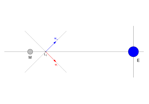
Figure 2: Convention of the eigenvectors of the hyperbolic part of $L_{1}$. Analogously for $L_{2}$.

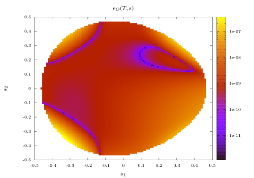
Figure 3: For the expansion of ${\mathcal{W}}^{cs}(L_{1})$ computed up to order 20, evaluation of the error in the orbit estimate $e_{O}$ for all points $\hat{s}$ in the mesh of $S_{1}^{h}$ satisfying $s_{4}=0$, $h=-1.5852$.

As a first example, a set of points in $S_{1}^{h}$ for $h=-1.586$ is computed using a parameterization of order 20 of ${\mathcal{W}}^{cs}(L_{1})$. For each point $(\hat{s},\delta)$ with $\hat{s}\in S^{h}_{1}$, the corresponding orbit error is computed. Figure 3 represents these errors as a color gradient map. For clarity, Figure 3 only shows the error for the points in the mesh of $S_{1}^{h}$ with $s_{4}=0$. With just these points it can be seen already that the error is quite heterogeneous in the energy level.

This procedure can be repeated for several energies and several orders of the expansions in order to determine which order we need to choose when computing the parameterizations for each energy level. In order to consider several energy levels, we take the maximum error of all the points of the mesh of an iso-energetic slice and plot the error as a function of energy. This is done in Figure 4 left, for ${\mathcal{W}}^{cs}(L_{1})$, and Figure 4 right, for ${\mathcal{W}}^{cu}(L_{2})$. Figure 4 shows how the error decreases with the order of the expansions, but at each order increases with energy. By using order 30, these figures show that we can reach a value of $h=-1.575$ in both libration points with error bounded by $10^{-4}$. So, from now on, all the computations will be done using expansions up to order 30.

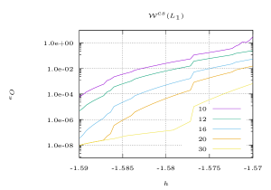
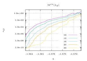
Figure 4: For the expansions of ${\mathcal{W}}^{cs}(L_{1})$ and ${\mathcal{W}}^{cu}(L_{2})$ computed up to indicated orders, evaluation of the maximum error estimate $e_{O}$ for $|\delta|=10^{-3}$, $|T|=3$ and different energy levels.

5 Computing heteroclinic connections

This section is devoted to introduce the main methodology to compute heteroclinic connections between center manifolds once the iso-energetic slices of center manifolds have been obtained. For this purpose, and as it was indicated in Section 3, the invariant manifolds ${\mathcal{W}}^{cs}(L_{1})$ and ${\mathcal{W}}^{cu}(L_{2})$ are considered and, at the same time, the meshes presented in Section 4 will be used as starting guesses.

Consider two (real) parameterizations for ${\mathcal{W}}^{cs}(L_{1})$ and ${\mathcal{W}}^{cu}(L_{2})$, computed according to Section 3, that will be denoted by ${\tilde{W}}^{(1)}(s)$ and ${\tilde{W}}^{(2)}(s)$, for $s$ in a neighborhood of the origin in $\mathbb{R}^{5}$. From the error explorations of the previous Section, for ${\tilde{W}}^{(1)}(s)$ and ${\tilde{W}}^{(2)}(s)$ to be accurate we need that $|s_{5}|\leq\delta:=10^{-3}$. Therefore, in order to obtain heteroclinic connections, and also according to the discussion on manifold branches of the previous Section, ${\mathcal{W}}^{cs}(L_{1})$ (resp. ${\mathcal{W}}^{cu}(L_{2})$) needs to be extended through numerical integration, starting from points ${\tilde{W}}^{(1)}(s)$ with $s_{5}=\delta^{s}:=-\delta$ (resp. ${\tilde{W}}^{(2)}(s)$ with $s_{5}=\delta^{u}:=\delta$).

Following [18, 17, 7, 1], we look for heteroclinic connections by trying to find intersections of ${\mathcal{W}}^{cs}(L_{1})$ and ${\mathcal{W}}^{cu}(L_{2})$ in an iso-energetic Poincaré section of energy $h$. This Poincaré section is given by an hypersurface $\Sigma:=\{g(Z)=0\}$ for $g\colon\mathbb{R}^{6}\longrightarrow\mathbb{R}$ that should be known to be intersected by ${\mathcal{W}}^{cs}(L_{1})$ and ${\mathcal{W}}^{cu}(L_{2})$ at the energy level $h$. Since the connections we are looking for are the ones that join the vicinities of $L_{1}$ and $L_{2}$, in our case it will be convenient to take $g(Z)=x-\mu+1$, for which $\Sigma$ is perpendicular to the $x$ axis and contains the the second primary of the RTBP. We will denote as $P^{\pm k}_{\Sigma}$ a Poincaré map associated to $\Sigma$, with $k$ being the number of crossings with the section and the sign indicating whether integration is done forward or backward in time. Recalling the $S^{h}_{j}$ sets defined in (14), heteroclinic connections are found by solving the following equation: find $\hat{s}^{u}\in S_{2}^{h},\hat{s}^{s}\in S_{1}^{h}$, such that

$$P_{\Sigma}^{-k}({\tilde{W}}^{(1)}(\hat{s}^{s},\delta^{s}))-P_{\Sigma}^{+l}({\tilde{W}}^{(2)}(\hat{s}^{u},\delta^{u}))=0.$$ (20)

The indexes $k$ and $l$ must be chosen in such a way that $k+l$ is an even number and any pair satisfying that $k+l=2n$ for some $n\in\mathbb{N}$ will give identical results.

Any root finding method to solve system (20) requires a good initial condition. In order to find such initial conditions, we first choose an energy level $h$ for which heteroclinic connections are expected to be found (see the next Section). For this energy level, we apply the meshing procedure of the previous Section in order to obtain points $\hat{S}^{h}_{1}\subset S^{h}_{1}$, $\hat{S}^{h}_{2}\subset S^{h}_{2}$. Then, the following sets are obtained:

$$\{P_{\Sigma}^{+l}({\tilde{W}}^{(2)}(\hat{s},\delta^{u}))\}_{\hat{s}\in\hat{S}^{h}_{2}},\quad\{P_{\Sigma}^{-k}({\tilde{W}}^{(1)}(\hat{s},\delta^{s}))\}_{\hat{s}\in\hat{S}^{h}_{1}}.$$

For each point on these sets we compute its Euclidean distance to every point of the other set and we store the minimum distance and the point from the other manifold that gives it. Then, for each $\hat{s}^{s}\in\hat{S}_{1}^{h}$, we obtain the triple $(\hat{s}^{s},\hat{s}^{u}(\hat{s}^{s}),d(\hat{s}^{s}))$ where

$$\begin{split}d(\hat{s}^{s})&:=\min_{\hat{s}^{u}\in\hat{S}_{2}^{h}}\text{dist}(P_{\Sigma}^{-k}({\tilde{W}}^{(1)}(\hat{s}^{s},\delta^{s})),P_{\Sigma}^{+l}({\tilde{W}}^{(2)}(\hat{s}^{u},\delta^{u}))),\\ \hat{s}^{u}(\hat{s}^{s})&:=\arg\min_{\hat{s}^{u}\in\hat{S}^{h}_{2}}\text{dist}(P_{\Sigma}^{-k}({\tilde{W}}^{(1)}(\hat{s}^{s},\delta^{s})),P_{\Sigma}^{+l}({\tilde{W}}^{(2)}(\hat{s}^{u},\delta^{u}))),\end{split}$$ (21)

this is, $\hat{s}^{u}(\hat{s}^{s})$ is the value of $\hat{s}^{u}$ that gives the minimum in the expression of $d(\hat{s}^{s})$. Note that the computation could also be done in terms of $\hat{s}^{u}\in\hat{S}_{2}^{h}$. By defining a numerical tolerance $\xi$, we can take pairs $(\hat{s}^{s},\hat{s}^{u}(\hat{s}^{s}))$ such that $d(\hat{s}^{s})\leq\xi$ as initial approximations to solve equation (20).

The system of equations we actually solve in order to find heteroclinic connections is not (20) but a modification of it. In order to avoid the computation of iterated Poincaré maps and their differentials, we add the equation of the Poincaré section to the system of equations to solve and we also introduce as unknowns $T^{s},T^{u}\in\mathbb{R}$, which are the corresponding times of flight from the points ${\tilde{W}}^{(1)}(\hat{s}^{s},\delta^{s})$ and ${\tilde{W}}^{(2)}(\hat{s}^{u},\delta^{u})$, respectively, to the section $\Sigma$. Since $T^{s},T^{u}$ may become large, and in order to maintain high precision, a multiple-shooting strategy is used: we add as unknowns new points $x_{0}^{s},\dots,x_{m^{s}}^{s}$ along the stable branch and additional points $x_{0}^{u},\dots,x_{m^{u}}^{u}$ along the unstable one. With that, and considering the corresponding matching equations in these variables, the following system of equations equivalent to (20) is obtained:

$$\begin{split}{\tilde{W}}^{(2)}(\hat{s}^{u},\delta^{u})-x_{0}^{u}&=0,\\ \Phi_{T^{u}/m^{u}}(x_{i}^{u})-x_{i+1}^{u}&=0,\qquad i=0,\dots,m^{u}-1,\\ {\tilde{W}}^{(1)}(\hat{s}^{s},\delta^{s})-x_{0}^{s}&=0,\\ \Phi_{T^{s}/m^{s}}(x_{i}^{s})-x_{i+1}^{s}&=0,\qquad i=0,\dots,m^{s}-1,\\ g(x_{m^{u}}^{u})&=0,\\ H(x_{m^{u}}^{u})-h&=0,\\ x_{m^{u}}^{u}-x_{m^{s}}^{s}&=0,\end{split}$$ (22)

for the set of unknowns

$$\hat{s}^{u},T^{u},x_{0}^{u},\dots,x_{m^{u}}^{u},\hat{s}^{s},T^{s},x_{0}^{s},\dots,x_{m^{s}}^{s}.$$ (23)

In spite of being apparently more cumbersome, a solver for this system is actually simpler to code than one for (20), since Poincaré maps are no longer explicitly present, and the introduction of multiple shooting points prevents the appearance of the parameterization composed in the flow. The differential of the flow is computed through numerical integration of the first variational equations.

In this system, the number of unknowns is $n(m^{u}+m^{s}+2)+2d$, while the number of equations is $n(m^{u}+m^{s}+3)+2$ so, for any values of $m^{u}$, $m^{s}$, we will have $2d-n-2$ more unknowns than equations. Particularly, for $n=6$ and $d=5$, this is 2 more unknowns than equations. Since, by a dimensional argument (and as numerically found in a similar problem [1]), the set of heteroclinic connections in an energy level is expected to be two-dimensional, having 2 more unknowns than equations is coherent with this fact, and system (22) should have full rank. Numerical checks with SVD (see e.g. [11]) have confirmed this last fact.

System (22) has been solved by performing minimum-norm lest-squares Newton corrections, that can be computed through QR decompositions with column pivoting ([19, 29]) as long as the dimensions of the kernel is known. This methodology addresses the fact that number of equations and unknowns is different. Moreover, from (22), several other systems of interest can be obtained by eliminating equations and/or fixing values of unknowns. For instance, one can fix $s_{3}^{s}=s_{4}^{s}=s_{3}^{u}=s_{4}^{u}=0$ in order to look for heteroclinic connections between planar Lyapunov p.o., thanks to the parameterization style we have used (see Section 3). All of these derived systems are easily coped with by the same routine.

6 Numerical results

In this section we apply all the developments of Sections 3, 4, 5 to the computation of whole sets of heteroclinic connections between center manifolds of $L_{1}$, $L_{2}$ of the spatial, circular RTBP in the Earth-Moon case for several energy levels. All the numerical integration has been performed through a Runge-Kutta-Felbergh method of orders 7 and 8 with relative tolerance $10^{-14}$. System (22) has been solved with absolute tolerance $10^{-10}$. All the explorations presented in this section have been carried out on a Fujitsu Celsius R940 workstation, with two 8-core Intel Xeon E5-2630v3 processors at 2.40GHz, running Debian GNU/Linux 11 with the Xfce 4.16 desktop. The source code has been written in C, compiled with GCC 10.2.1 and linked against LAPACK 3.7.0. The code also uses OpenMP $4.0$ in order to parallelize most of the computations. All the computational times presented in this Section refer to total computing (user) time, accounting for all the cores. In the workstation mentioned, wall-clock time is roughly user time divided by 16.

As mentioned in Section 5, system (22) is easily modified in order to look for heteroclinic connections of planar Lyapunov orbits. When such connections exist, heteroclinic connections between tori are expected to be found nearby. As done in previous works [17, 7], we start by looking for connections between planar Lyapunov p.o. by fixing $k=1$ for a set of different energy levels and varying $j$ until the manifold tubes of the departing and arriving p.o. of the energy level seem to intersect at $\Sigma=\{x=\mu-1\}$. Since neither the planar Lyapunov p.o. nor their stable and unstable manifolds have $z,p_{z}$ components (this is, they are planar), this is easily visualized in an $xy$ projection. A $yp_{y}$ projection of the Poincaré sections of the manifold tubes can confirm if the manifold tubes intersect or not.

Figure 5 is a sample of results related to the search of heteroclinic connections of planar Lyapunov p.o. The left column displays $xy$ projections of the manifold tubes, whereas the right column displays $yp_{y}$ projections of the Poincaré sections of the manifold tubes. The energies have been chosen in such a way that $2$ heteroclinic connections of p.o. exist. It can be seen that, as energy increases, the planar Lyapunov p.o. around $L_{2}$ becomes bigger. Its unstable manifold tube also becomes bigger, in such a way that, with a smaller value of $j$, this tube is able to intersect the stable manifold tube of the planar Lyapunov p.o. around $L_{1}$. This happens when going from the first to the second row of Figure 5, and from the second to the third. Observe also that some sections of the manifold tubes are not represented as closed curves in the $yp_{y}$ projections of the right column of Figure 5. This is because of their proximity to the Moon: we have stopped numerical integration at two radii distance of its center. This can be also appreciated in the $xy$ plots of the left column of Figure 5.

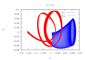
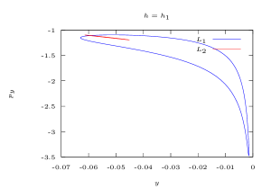
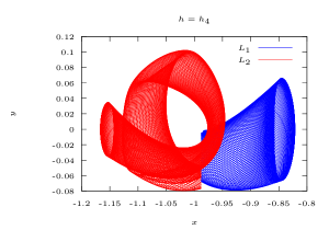
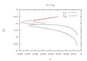
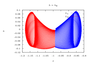
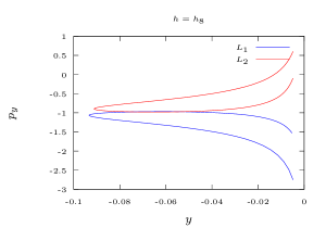
Figure 5: Numerical explorations of the unstable and stable branches of the planar Lyapunov p.o. for the energy levels $h_{1}$, $h_{4}$ and $h_{8}$ and $j=1,3,5$ crossings. Left: $xy$ view of the 2-dimensional manifold tubes up to the Poincaré section $\Sigma$. Right: Poincaré section of the 2-dimensional manifold tubes in the $yp_{y}$ plane projection. The values $\{h_{i}\}_{i=1}^{9}$ are given in Table 2.

When looking for heteroclinic connections of planar Lyapunov p.o. we only consider primary heteroclinics, in the sense that they correspond to the first intersection of the manifold tubes. Further intersections are possible, giving rise to “higher-order” heteroclinics. E.g., when in the middle row of Figure 5 we locate heteroclinic connections for $j=3$, the heteroclinic connections for $j=5$ still exist. But they are very tangled, with one manifold tube performing infinite loops around the other (see [3] for some discussion of this phenomenon). Nearby heteroclinic connections between tori should inherit this complicated geometry. They will not be considered here.

In view of Figure 5, we set as goal the description of the whole set of heteroclinic connections from ${\mathcal{W}}^{c}(L_{2})$ to ${\mathcal{W}}^{c}(L_{1})$ for nine energy levels that, in groups of three, correspond to each of the behaviors of the manifold tubes shown in this figure. The energy levels chosen are shown in Table 2, and will be globally denoted as $\{h_{i}\}_{i=1}^{9}$.

$$\begin{array}[]{c|r@{}c@{}l|c|c}i&\lx@intercol\hfil h_{i}\hfil\lx@intercol\vrule\lx@intercol&j&k\\ \hline\cr 1&-1&.&58606&1&5\\ 2&-1&.&5855&1&5\\ 3&-1&.&585&1&5\end{array}\qquad\begin{array}[]{c|r@{}c@{}l|c|c}i&\lx@intercol\hfil h_{i}\hfil\lx@intercol\vrule\lx@intercol&j&k\\ \hline\cr 4&-1&.&5845&1&3\\ 5&-1&.&5844&1&3\\ 6&-1&.&5843&1&3\end{array}\qquad\begin{array}[]{c|r@{}c@{}l|c|c}i&\lx@intercol\hfil h_{i}\hfil\lx@intercol\vrule\lx@intercol&j&k\\ \hline\cr 7&-1&.&5755&1&1\\ 8&-1&.&575&1&1\\ 9&-1&.&574&1&1\end{array}$$

Table 2: Energy levels $\{h_{i}\}_{i=1}^{9}$ for which the set of heteroclinic connections from ${\mathcal{W}}^{c}(L_{2})$ to ${\mathcal{W}}^{c}(L_{1})$ is to be found.

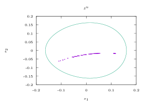
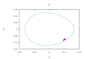
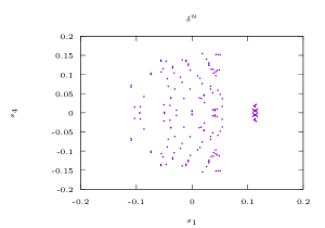
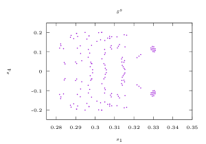
Figure 6: “Low-res” heteroclinic connection set from ${\mathcal{W}}^{c}(L_{2})$ to ${\mathcal{W}}^{c}(L_{1})$ for the energy level $h=h_{3}$ (purple) in terms of $\hat{s}^{u}\in S_{2}^{h}$ (left) and $\hat{s}^{s}\in S_{1}^{h}$ (right) from (23). Green: planar Lyapunov p.o., included as a reference.

In order to give an idea of the steps to follow and the computational effort required, we provide the details of the computation of the set of heteroclinic connections for $h=h_{3}$, with $k=1$ and $j=5$. The corresponding iso-energetic slices $S^{h}_{1}$, $S^{h}_{2}$ (see eq. (14)) are meshed according to Section 4. The $\hat{S}^{h}_{1}$ mesh spacing in $s_{1},s_{2},s_{4}$ is of $0.0079$ units, with a total of $2049031$ points that are obtained in $16106$ seconds. The $\hat{S}^{h}_{2}$ mesh spacing is $0.0034$, with a total of $826599$ points that are obtained in $6742$ seconds. Setting a tolerance $\xi=10^{-4}$ gives a set of pairs $(\hat{s}^{s},\hat{s}^{u})$ as initial approximations of heteroclinic connections that are later refined using system (22) as explained in Section 5. The set of heteroclinic connections obtained are presented in Figure 6 in terms of the values of $\hat{s}^{u},\hat{s}^{s}$ found solving system (22). This set, made of 168 connections, that have been refined in 68 seconds, provides a “low-res” representation of the total heteroclinic connection set.

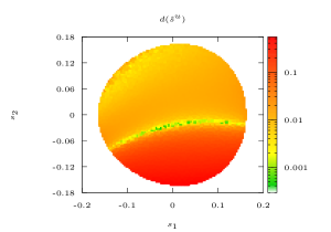
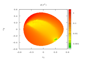
Figure 7: Color gradient map provided by equation (21) for the iso-energetic slice of the center manifold at $h=h_{3}$.

Aiming to refine these results, and in order to describe the whole set of heteroclinic connections, the values $d(\hat{s}^{s})$ are computed for $\hat{s}^{s}$ varying on the mesh of $S^{h}_{1}$ according to the expression (21), and the values $d(\hat{s}^{s})$ are computed for $\hat{s}^{s}$ varying on the mesh of $S^{h}_{2}$ according to an analogous expression. These values are represented as gradient maps in Figure 7. These figures are useful to determine which regions over each $S_{j}^{h}$ need to be re-meshed with a finer grid. We have used a different re-meshing strategy depending of the shape of these regions. In the case of Figure 7 right, a bounding rectangle in $s_{1},s_{2}$. In the case of Figure 7 left, in which the region seems to be “stretched along a curve”, this curve is approximated by a degree 5 interpolating polynomial $s_{2}=p(s_{1})$ that is then fattened in $s_{2}$. In both cases, $s_{4}$ is allowed to range between the minimum and maximum values attained in the low-res representation of the set of connections of Figure 6. Once these regions are re-meshed, they are propagated again up to the Poincaré section, and the triples $(\hat{s}^{s},\hat{s}^{u}(\hat{s}^{s}),d(\hat{s}^{s}))$ are computed again. From these triples, and fixing again a tolerance $\xi=10^{-3}$, a new set of initial approximations to heteroclinic connections is found, which, through the solution of system (22), is refined to a set of true connections up to tolerance of $10^{-10}$. Thus obtaining 45390 connections in a total of 17628 seconds. The results are shown in Figure 8.

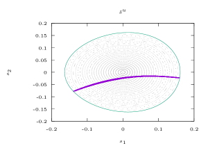
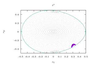
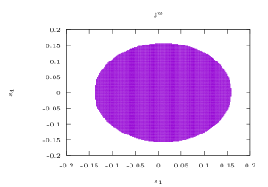
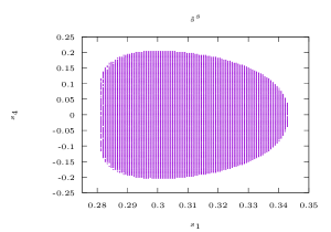
Figure 8: Whole set of heteroclinic connections for the energy level $h=h_{3}$ from ${\mathcal{W}}^{c}(L_{2})$ to ${\mathcal{W}}^{c}(L_{1})$ (purple). Green: planar Lyapunov p.o., included as a reference. Grey: Poincaré sections of several trajectories at $\Sigma:=\{s_{4}=0\}$.

Figure 8 is a first figure that could be of special interest for a space mission analyst. As an addition to Figure 6, and following the classical representations of [12, 23], the $\{s_{4}=0\}$ Poincaré sections of several trajectories of the energy level have been represented in grey in the first row of Figure 8. In this way, Lyapunov and Halo periodic orbits are seen as fixed points ($s_{1}=s_{2}=0$ corresponds to the vertical Lyapunov p.o. and the two other points correspond to the Halo orbits of the energy level), and invariant tori are seen as invariant curves (tori can be found from the Lissajous and quasi-halo families). From the right column of Figure 8, it can be seen that, for this energy level, a small range of the tori close to the planar Lyapunov p.o. around $L_{1}$ are connected to most of the tori around $L_{2}$. So, assuming this energy level is convenient, the small range of tori close to the planar p.o. would be the place for a space servicing station, that would have “free routes” (through the heteroclinic connections) to most of the tori around $L_{2}$ (always in the $h_{3}$ energy level). By converting all the points of these figures to synodic coordinates and using the same scale in both axes, even an idea of the physical shape of the connected tori could be inferred.

Still considering applications to mission analysis, the last row of Figure 8 would be useful as well. In the last step of its computation, namely the solution of system (22), the coordinates $s_{1},s_{4}$ in either ${\mathcal{W}}^{cs}(L_{1})$ or ${\mathcal{W}}^{cu}(L_{2})$ can be kept constant during Newton iterations, and, in this way, obtain an equally spaced set of points inside the region of heteroclinic connections. This has actually been done in the second row of Figure 8. Over these diagrams, properties of interest of the connection (such as time of flight, $z$-amplitude, minimum distance to the Moon) could be graphed.

From Figure 8, it could seem that the set of heteroclinic connections is a 2-dimensional surface with boundary. This is not the case: in the re-meshing of the connection candidates, for most of them two solutions are found for the $s_{3}$ coordinate. Many survive as heteroclinic connections. If we use the $s_{3}$ coordinate in the plot of the set of heteroclinic connections, a topological sphere is obtained (see Figure 9). This is coherent with the results in [1]. This is also coherent with the fact that the surfaces of connections displayed in Figure 8 have its apparent boundary on the boundary of the solid perturbed ellipsoid of the $s_{1}s_{2}s_{4}$ projection of $S_{1}^{h}$, $S_{2}^{h}$. For $S_{2}^{h}$, this fact can be appreciated in Figure 10, where the mesh obtained for this perturbed ellipsoid is represented both in center manifold and synodic coordinates. The representation in synodic coordinates of Figure 10 uses the same scale in all axes, and, in this way, provides the actual physical appearance in configuration space of an iso-energetic slice of the center manifold.

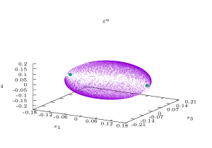
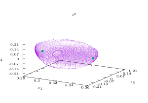
Figure 9: Whole set of heteroclinic connections from ${\mathcal{W}}^{c}(L_{2})$ to ${\mathcal{W}}^{c}(L_{1})$ for the energy level $h=h_{3}$ (purple). Green: heteroclinic connections between the planar Lyapunov p.o. at the same energy.

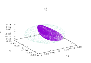
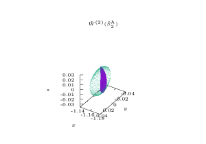
Figure 10: Representation of the boundary of the obtained mesh for the perturbed ellipsoid $S_{2}^{h}$ at $h=h_{3}$ (green) together with the heteroclinic connections $\hat{s}^{u}\in S_{2}^{h}$ from ${\mathcal{W}}^{c}(L_{2})$ to ${\mathcal{W}}^{c}(L_{1})$ (purple). Left: representation in the center manifold. Right: representation in synodic coordinates.

In Figure 11 we represent the whole set of connections from ${\mathcal{W}}^{c}(L_{2})$ to ${\mathcal{W}}^{c}(L_{1})$ for the energies $h_{3},h_{6},h_{9}$, by choosing in each case a 3D projection suitable to better see them as topological spheres. The two heteroclinic connections between the planar Lyapunov p.o. of the energy level are shown as points in the same plot. As an illustration of how individual connections look like, for the energies $h_{2}$, $h_{5}$, $h_{7}$ we represent the $xy$ and $yz$ projections of the connections passing by the moon at minimum distance (Figure 13), and also the connections having maximum $z$-amplitude (Figure 14). In order to show the true physical appearance of these connections, the same scale has been used in both axes in all the plots. For the same reason, the Moon has been added to the $xy$ projections.

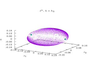
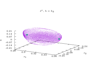
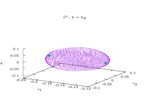
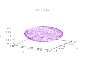
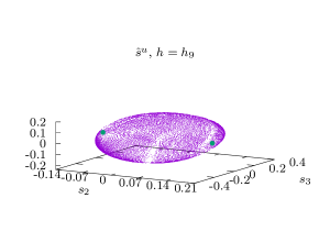
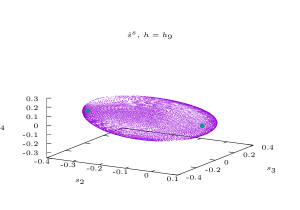
Figure 11: Representation of the whole set of heteroclinic connections from ${\mathcal{W}}^{c}(L_{2})$ to ${\mathcal{W}}^{c}(L_{1})$ (purple) for several energy levels $h_{i}$, $i=3,6,9$, and in terms of $\hat{s}^{u}\in S_{2}^{h}$ (left) and $\hat{s}^{s}\in S_{1}^{h}$ (right) from (23). Green: heteroclinic connections between planar Lyapunov p.o..

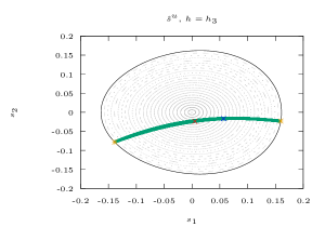
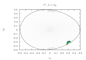
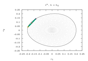
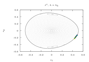
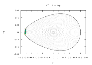
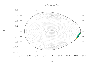
Figure 12: Representation of the whole set of heteroclinic connections from ${\mathcal{W}}^{c}(L_{2})$ to ${\mathcal{W}}^{c}(L_{1})$ (green) for the energy levels $h_{i}$, $i=3,5,7$, and in terms of $\hat{s}^{u}\in S_{2}^{h}$ (left) and $\hat{s}^{s}\in S_{1}^{h}$ (right) from (23). Yellow: heteroclinic connections between planar Lyapunov p.o.. Black: planar Lyapunov p.o., included as reference. Grey: Poincaré sections of several trajectories at $\Sigma:=\{s_{4}=0\}$. Blue: initial condition of the heteroclinic connection with minimum distance presented in Figure 13. Red: initial condition of the heteroclinic connection with maximum $z$-amplitude presented in Figure 14.

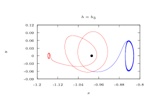
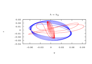
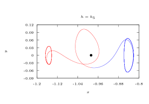
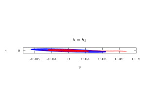
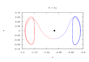
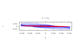
Figure 13: Heteroclinic connection from ${\mathcal{W}}^{c}(L_{2})$ to ${\mathcal{W}}^{c}(L_{1})$ with minimum distance to the second primary along the trajectory at different energy levels $h_{i}$, $i=3,5,7$. Red: unstable branch of $L_{2}$. Blue: stable branch of $L_{1}$.

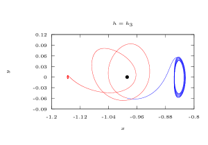
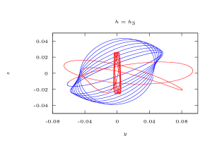
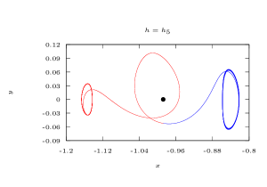
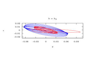
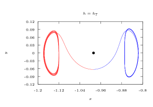
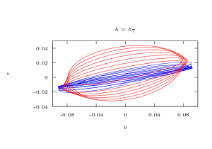
Figure 14: Heteroclinic connection from ${\mathcal{W}}^{c}(L_{2})$ to ${\mathcal{W}}^{c}(L_{1})$ with maximum $z$-amplitude along the trajectory at different energy levels $h_{i}$, $i=3,5,7$. Red: unstable branch of $L_{2}$. Blue: stable branch of $L_{1}$.

7 Conclusions

In this paper we have shown how to compute whole sets of heteroclinic connections between iso-energetic slices of center manifolds of fixed points of center$\times$center$\times$saddle type of autonomous, 3-degrees of-freedom Hamiltonians. To do so, we have used the parameterization method by adding a new extra style to uncouple the hyperbolic part from the central and thus making explicit the fibered structure of center-stable and center-unstable manifolds. A meshing strategy for iso-energetic slices of center manifolds that avoids numerical integration of the reduced equations is crucial for the whole procedure to be computationally efficient.

This methodology is applied to the Earth-Moon spatial, circular RTBP to obtain whole sets of heteroclinic connections from the center manifold of $L_{2}$ to the center manifold of $L_{1}$ for different energy levels. As explained, these sets contain a full description of the connections between different objects from the departure center manifold to the arrival center manifold and that is why we expect these sets to be useful in preliminary mission design. Some comments in this direction have been made.

The applicability of the procedure presented in this paper is limited by the validity of the expansions of center-stable and center-unstable manifolds. In this paper, for the Earth-Moon case, they have been checked to be accurate up to energies in which the $L_{1}$ Halo family of periodic orbits has already appeared and has a certain non-small amplitude (Figures 4,12). A starting point in order to go to higher energies would be to numerically globalize the center-stable and center-unstable manifolds of the libration points. This can be done from a sufficiently dense grid of numerically computed invariant tori together with their stable and unstable manifolds [31, 30]. There are several methodologies available for the numerical computation of invariant tori and their manifolds [19, 2, 21, 25], of which the ones based on the parameterization method and flow maps (or stroboscopic maps) seem to be the most efficient computationally.

References

- [1] L. Arona and J. J. Masdemont. Computation of heteroclinic orbits between normally hyperbolic invariant 3-spheres foliated by 2-dimensional invariant tori in Hill’s problem. Discrete Contin. Dyn. Syst., (Dynamical Systems and Differential Equations. Proceedings of the 6th AIMS International Conference, suppl.):64–74, 2007.
- [2] N. Baresi, Z. P. Olikara, and D. J. Scheeres. Fully numerical methods for continuing families of quasi-periodic invariant tori in astrodynamics. The Journal of the Astronautical Sciences, 2018.
- [3] E. Barrabés, J.-M. Mondelo, and M. Ollé. Numerical continuation of families of homoclinic connections of periodic orbits in the RTBP. Nonlinearity, 22(12):2901–2918, 2009.
- [4] X. Cabré, E. Fontich, and R. de la Llave. The parameterization method for invariant manifolds. I. Manifolds associated to non-resonant subspaces. Indiana Univ. Math. J., 52(2):283–328, 2003.
- [5] X. Cabré, E. Fontich, and R. de la Llave. The parameterization method for invariant manifolds. II. Regularity with respect to parameters. Indiana Univ. Math. J., 52(2):329–360, 2003.
- [6] X. Cabré, E. Fontich, and R. de la Llave. The parameterization method for invariant manifolds. III. Overview and applications. J. Differential Equations, 218(2):444–515, 2005.
- [7] E. Canalias and J. J. Masdemont. Homoclinic and heteroclinic transfer trajectories between planar Lyapunov orbits in the sun-earth and earth-moon systems. Discrete Contin. Dyn. Syst. Series A, 14(2):261–279, 2006.
- [8] C. C. Conley. Low energy transit orbits in the restricted three-body problem. SIAM J. Appl. Math., 16:732–746, 1968.
- [9] A. Delshams, J. Masdemont, and P. Roldan. Computing the scattering map in the spatial Hill’s problem. Discrete and Continuous Dynamical Systems, series B, 10(2, 3):455–483, 2008.
- [10] D. W. Dunham and R. W. Farquhar. Libration point missions, 1978–2002. In G. Gómez, M. W. Lo, and J. J. Masdemont, editors, Libration Point Orbits and Applications, Singapore, 2003. World Scientific. Proceedings of the conference Libration Point Orbits and Applications, Aiguablava (Girona, Spain), June 10–14, 2002.
- [11] G. H. Golub and C. F. van Loan. Matrix Computations. The Johns Hopkins University Press, Baltimore and London, 3rd edition, 1996.
- [12] G. Gómez, À. Jorba, J. Masdemont, and C. Simó. Dynamics and Mission Design Near Libration Point Orbits – Volume 3: Advanced Methods for Collinear Points. World Scientific, 2001. Reprint of ESA Report Study Refinement of Semi–Analytical Halo Orbit Theory, 1991.
- [13] G. Gómez, À. Jorba, J. Masdemont, and C. Simó. Dynamics and Mission Design Near Libration Point Orbits – Volume 4: Advanced Methods for Triangular Points. World Scientific, 2001. Reprint of ESA Report Study of Poincaré Maps for Orbits Near Lagrangian Points, 1993.
- [14] G. Gómez, W. S. Koon, M. W. Lo, J. E. Marsden, J. Masdemont, and S. D. Ross. Connecting orbits and invariant manifolds in the spatial restricted three-body problem. Nonlinearity, 17(5):1571–1606, 2004.
- [15] G. Gómez, J. Llibre, R. Martínez, and C. Simó. Dynamics and Mission Design Near Libration Point Orbits – Volume 1: Fundamentals: The Case of Collinear Libration Points. World Scientific, 2001. Reprint of ESA Report Station Keeping of Libration Point Orbits, 1985.
- [16] G. Gómez, J. Llibre, R. Martínez, and C. Simó. Dynamics and Mission Design Near Libration Point Orbits – Volume 2: Fundamentals: The Case of Triangular Libration Points. World Scientific, 2001. Reprint of ESA Report Study on Orbits near the Triangular Libration Points in the Perturbed Restricted Three–Body Problem, 1987.
- [17] G. Gómez, M. Marcote, and J.-M. Mondelo. The invariant manifold structure of the spatial Hill’s problem. Dynamical Systems. An International Journal, 20(1):115–147, 2005.
- [18] G. Gómez and J. J. Masdemont. Some zero cost transfers between Libration Point orbits. Advances in the Astronautical Sciences, 105:1199–1216, 2000.
- [19] G. Gómez and J.-M. Mondelo. The dynamics around the collinear equilibrium points of the RTBP. Phys. D, 157(4):283–321, 2001.
- [20] A. Haro, M. Canadell, J.-L. Figueras, A. Luque, and J. M. Mondelo. The parameterization method for invariant manifolds: from rigorous results to effective computations, volume 195 of Applied Mathematical Sciences. Springer, 2016.
- [21] A. Haro and J. M. Mondelo. Flow map parameterization methods for invariant tori in Hamiltonian systems. Commun. Nonlinear Sci. Numer. Simul., 101:Paper No. 105859, 34, 2021.
- [22] K. C. Howell, B. T. Barden, R. S. Wilson, and M. W. Lo. Trajectory Design Using a Dynamical Systems Approach With Application to Genesis. Technical Report 97–0985, Jet Propultion Laboratory, 1997.
- [23] À. Jorba and J. J. Masdemont. Dynamics in the center manifold of the Restricted Three–Body Problem. Physica D, 132:189–213, 1999.
- [24] W. S. Koon, M. W. Lo, J. E. Marsden, and S. D. Ross. Heteroclinic connections between periodic orbits and resonance transitions in celestial mechanics. Chaos, 10(2):427–469, 2000.
- [25] B. Kumar, R. L. Anderson, and R. de la Llave. Rapid and accurate methods for computing whiskered tori and their manifolds in periodically perturbed planar circular restricted 3-body problems. CELESTIAL MECHANICS & DYNAMICAL ASTRONOMY, 134(1), FEB 2022.
- [26] J. Masdemont. High-order expansions of invariant manifolds of libration point orbits with applications to mission design. Dynamical Systems: An International Journal, 20(1):59–113, March 2005.
- [27] R. P. McGehee. Some homoclinic orbits for the restricted three-body problem. PhD thesis, University of Wisconsin, 1969.
- [28] K. R. Meyer, G. R. Hall, and D. Offin. Introduction to Hamiltonian Dynamical Systems and the –Body Problem. Springer–Verlag, 2nd edition, 2009.
- [29] J.-M. Mondelo. Computing invariant manifolds for libration point missions. In G. Baù, A. Celletti, C. B. Galeș, and G. F. Gronchi, editors, Satellite Dynamics and Space Missions, pages 159–223, Cham, 2019. Springer International Publishing.
- [30] J.-M. Mondelo, E. Barrabés, G. Gómez, and M. Ollé. Fast numerical computation of Lissajous and quasi–halo libration point trajectories and their invariant manifolds. Paper IAC-12,C1,6,9,x14982. Proceedings of the 63rd International Astronautical Congress, 1-5 October 2012, Naples, Italy.
- [31] J.-M. Mondelo, E. Barrrabés, G. Gómez, and M. Ollé. Automatic generation of Lissajous–type Libration Point trajectories and its manifolds for large energies. Proceedings of the 21th International Symposium on Space Flight Dynamics, Toulouse (France) Sept. 28–Oct. 2, 2009.
- [32] L. M. Perko. Differential equations and dynamical systems. Springer-Verlag, New York, second edition, 1996.
- [33] C. L. Siegel and J. K. Moser. Lectures on celestial mechanics. Classics in Mathematics. Springer-Verlag, Berlin, 1995. Translated from the German by C. I. Kalme, Reprint of the 1971 translation.
- [34] E. M. Standish. JPL planetary and lunar ephemerides, DE405/LE405. Technical Report IOM 312.F.98-048, Jet Propultion Laboratory, 1998.
- [35] T. Sweetser, S. Broschart, V. Angelopoulos, G. Whiffen, D. Folta, M.-K. Chung, S. Hatch, and M. Woodard. ARTEMIS mission design. Space Sci Rev, 165:27–57, 2011.
- [36] V. Szebehely. Theory of orbits. The Restricted Problem of Three Bodies. Academic Press, 1967.
- [37] D. Wilczak and P. Zgliczynski. Heteroclinic connections between periodic orbits in the planar restricted circular three body problem. a computer assisted proof. Commun. Math. Phys., 234:37–75, 2003.
- [38] D. Wilczak and P. Zgliczynski. Heteroclinic connections between periodic orbits in the planar restricted circular three body problem. part ii. Commun. Math. Phys., 259:561–576, 2005.