Self-Organization Towards $1/f$ Noise in Deep Neural Networks

Abstract

Despite $1/f$ noise being ubiquitous in both natural and artificial systems, no general explanations for the phenomenon have received widespread acceptance. One well-known system where $1/f$ noise has been observed in is the human brain, with this ‘noise’ proposed by some to be important to the healthy function of the brain. As deep neural networks (DNNs) are loosely modelled after the human brain, and as they start to achieve human-level performance in specific tasks, it might be worth investigating if the same $1/f$ noise is present in these artificial networks as well. Indeed, we find the existence of $1/f$ noise in DNNs - specifically Long Short-Term Memory (LSTM) networks modelled on real world dataset - by measuring the Power Spectral Density (PSD) of different activations within the network in response to a sequential input of natural language. This was done in analogy to the measurement of $1/f$ noise in human brains with techniques such as electroencephalography (EEG) and functional Magnetic Resonance Imaging (fMRI). We further examine the exponent values in the $1/f$ noise in “inner” and “outer” activations in the LSTM cell, finding some resemblance in the variations of the exponents in the fMRI signal. In addition, comparing the values of the exponent at “rest” compared to when performing “tasks” of the LSTM network, we find a similar trend to that of the human brain where the exponent while performing tasks is less negative.

I Introduction

Noise is an often unwanted phenomenon in many different systems such as audio systems, electrical systems, communications, and in measurements. A common type of noise is $1/f$ noise, or pink noise, characterised by a power spectral density (PSD) $S(f)$ that is inversely proportional to frequency: $S(f)=kf^{-1}+C$. While there are relatively simple generative and stochastic models that explain other common types of noise such as white noise Åström (1970); Bass (2011) or Brownian noise Bass (2011), there are no such models for $1/f$ noise in general.

I.1 Sources of $1/f$ Noise

$1/f$ noise has since been found and characterised in a variety of electrical systems, including ionic solutions Hooge and Gaal (1971), diodes and PN junctions van der Ziel (1970), field effect transistors Fu and Sah (1972), and superconducting Josephson junctions Mück et al. (2005). In these systems, the definition of $1/f$ noise has been expanded to include noise with a spectral density proportional to $f^{\beta}$, with $-2<\beta<0$. In this paper, the term $1/f$ noise will be used to refer to these $1/f$-like signals that have an exponent $\beta$ smaller than 0 (white noise) and greater than -2 (Brownian noise).

Other than flicker noise in electronics, $1/f$ noise is ubiquitous in many physical systems, both natural and man-made. This pattern has been found in undersea currents Taft et al. (1974), global climate data Moon et al. (2018), Nile river flood and minimum levels Mandelbrot and Wallis (1968, 1969), sunspot frequency Mandelbrot and Wallis (1969), and many other natural processes Mandelbrot and Wallis (1969). Interestingly, $1/f$ noise is also present in man-made systems such as traffic systems Musha and Higuchi (1978); Nagatani (1993), concrete structures Carpinteri et al. (2018), and surprisingly, even in canonical examples of man-made “data” such as in music and speech Voss and Clarke (1978).

Another interesting source of $1/f$ noise is in biological systems, such as human heart rate fluctuations, where the spectrum for a healthy human is $1/f$, while that for someone with heart disease is closer to Brownian Peng et al. (1993); Struzik et al. (2004). $1/f$ noise is also found in other biological systems such as in giant squid axons Musha et al. (1981), human optical cells Medina and Díaz (2012), and in activity scans of the human brain Novikov et al. (1997).

I.2 Motivation

Despite the extraordinary ubiquity of $1/f$ noise and it being studied in many different fields for almost a century now, there is still no universal description for its occurrence, only specific models made to explain specific processes such as in diodes Schottky (1926); van der Ziel (1970) or other electronic components Christensen and Pearson (1936). Such a search is spurred by similar phenomena in other parts of statistical mechanics, such as the universal critical exponents in different universality classes Zinn-Justin (2002); Ódor (2004); Creswick and Kim (1997). As such, many believe that there is a similar universality in $1/f$ noise, and there is thus a great interest amongst many towards finding a deep all-encompassing explanation for the phenomenon.

One way of working towards that goal is to probe the areas where this $1/f$ noise is present in order to add to the pool of knowledge we have about this phenomenon. If a $1/f$ signal is persistent across both a system and a simpler analogue of it, one might be able to gain insight about the origin of the noise by studying the simpler system instead.

One such pair of analogues is the previously mentioned $1/f$ noise in the human brain, and the relatively less complex systems of deep neural networks (DNNs). While the neurons and connections in a DNN are many orders of magnitude less complex than those in the human brain, the general principle of operation of a DNN approximates that of a basic brain with simple connections Aggarwal (2018).

Similar to the human heart, $1/f$ noise presents itself strongly in the human brain He (2014). Like in the heart, the $1/f$ noise in the human brain presents itself differently in a healthy human brain compared to a brain with neurological conditions like schizophrenia Racz et al. (2021). While the study of this form of brain activity is in its early stages due to the $1/f$ signal being regarded as extraneous noise in the past, it has been proposed that the $1/f$ noise in the brain is important in regulating function and serves other cognitive purposes He et al. (2010).

With the fast progress of artificial neural networks, or deep neural networks (DNN) in particular, these artificial neural systems are fast approaching the human cognition level. As such, it would be appropriate for an analysis of the presence of $1/f$ noise in a DNN to include networks that approach a human level of competency. If this phenomenon also exists in DNN, the controllability and manipulability of the DNN would serve as a better experimental subject to further examine the origin of $1/f$ noise than the brain.

I.3 $1/f$ noise in the human brain

Brain activity can be measured in multiple different ways, such as non-invasive scalp electroencephalography (EEG) and functional magnetic resonance imaging (fMRI). These neuroimaging techniques detect different properties of the brain as a proxy for brain activity, which results in detection of different types of activity in different parts of the brain.

Scalp EEGs map brain activity by measuring electrical signals with electrodes placed on the scalp. These electrodes detect voltage fluctuations relative to a reference potential Niedermeyer (2017). Due to the positioning of the detectors outside the skull, the signals obtained for scalp EEGs are dominated by brain activity on the surface of the brain rather than in the bulk of the brain Niedermeyer (2017).

$1/f$ noise has shown up in the recordings of EEGs for decades He (2014). Once considered an unwelcome signal to be filtered out as background or instrumental noise, there is now significant interest and research into the role of $1/f$ noise in a healthy functioning brain He et al. (2010); Racz et al. (2021). Numerous studies have measured the scaling exponent $\beta$ of EEGs with similar results Dehghani et al. (2010); Pathania et al. (2021). The aggregate results obtained in Dehghani et al. (2010) gives a scaling exponent $\beta=-1.33\pm 0.19$, demonstrating $1/f$ noise.

Another form of neuroimaging is with fMRI which tracks blood flow through the brain Huettel et al. (2008). It has been shown that brain activity is linked to blood flow through the activated regions of the brain Logothetis et al. (2001), and this fact is the basis of how the images formed by fMRI are linked to brain activity. When mapping the fMRI signal to neural activity by comparing it to other methods of measuring electrical activity in the brain, it has been found that the fMRI signal mainly reflects the activity within the individual neurons rather than the outputs between the neurons Huettel et al. (2008).

Similar to in EEGs, $1/f$ noise also shows up in fMRI recordings He (2014, 2011). The scaling exponents measured in these studies are less negative than those in EEGs, with an average scaling exponent of $\beta=-0.84$. This exponent became even less negative when the brain performs tasks, averaging to $\beta=-0.72$ across the brain.

I.4 Recurrent Neural Networks

Recurrent Neural Networks (RNNs) are a type of DNN that preserve the state of an input across a temporal sequence by feeding the outputs of some nodes back into those same nodes. This is as opposed to feedforward DNNs, where data flows only from layer to layer. By retaining knowledge of previous inputs through this recurrence, RNNs are significantly more adept than simple feedforward networks at processing sequential data.

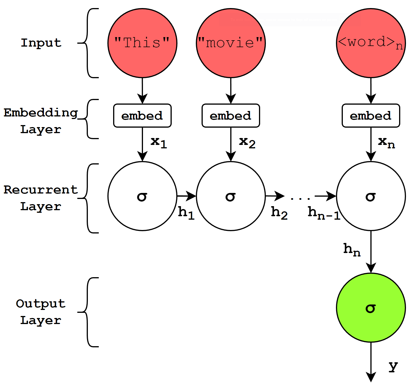
Figure 1: A (many-to-one) recurrent neural network visualised in its temporally unrolled representation. A time series (in this case a movie review with $n$ words) is input into the network sequentially. For each timestep $t$, the $t$th word passes into the embedding layer, which converts the word into a vector using a learned representation of a continuous vector space. The vector $\mathbf{x}_{t}$ then passes into the recurrent layer, which accepts both $\mathbf{x}_{t}$ and the output of itself from the previous timestep, $\mathbf{h}_{t-1}$. The recurrent layer then passes its output, $\mathbf{h}_{t}$, into itself for the next timestep. At the final timestep $n$, the recurrent layer passes its output $\mathbf{h}_{n}$ to the output layer which converts it to the output $\mathbf{y}$.

Table 1: Hyperparameters selected for the LSTM networks

Size of embedding layer	Size of LSTM layer	Training batch size	Dropout factor	L2 regularisation factor	Learning rate
32	60	128	0.1	0.001	0.005

Figure 1 shows the most basic form of an RNN, demonstrating the idea that these recurrent networks are deep through time, in contrast to the depth through layers of a simple feedforward network. However, this also means that the simple RNN suffers from the same problem as DNNs with large depths - the vanishing gradient problem. RNNs strugle to converge for particularly long input sequences of more than 10s of timesteps. In a way, RNNs are similar to the human brain at an abstract level, as the human brain continuously receives information and processes it using our biological neural networks.

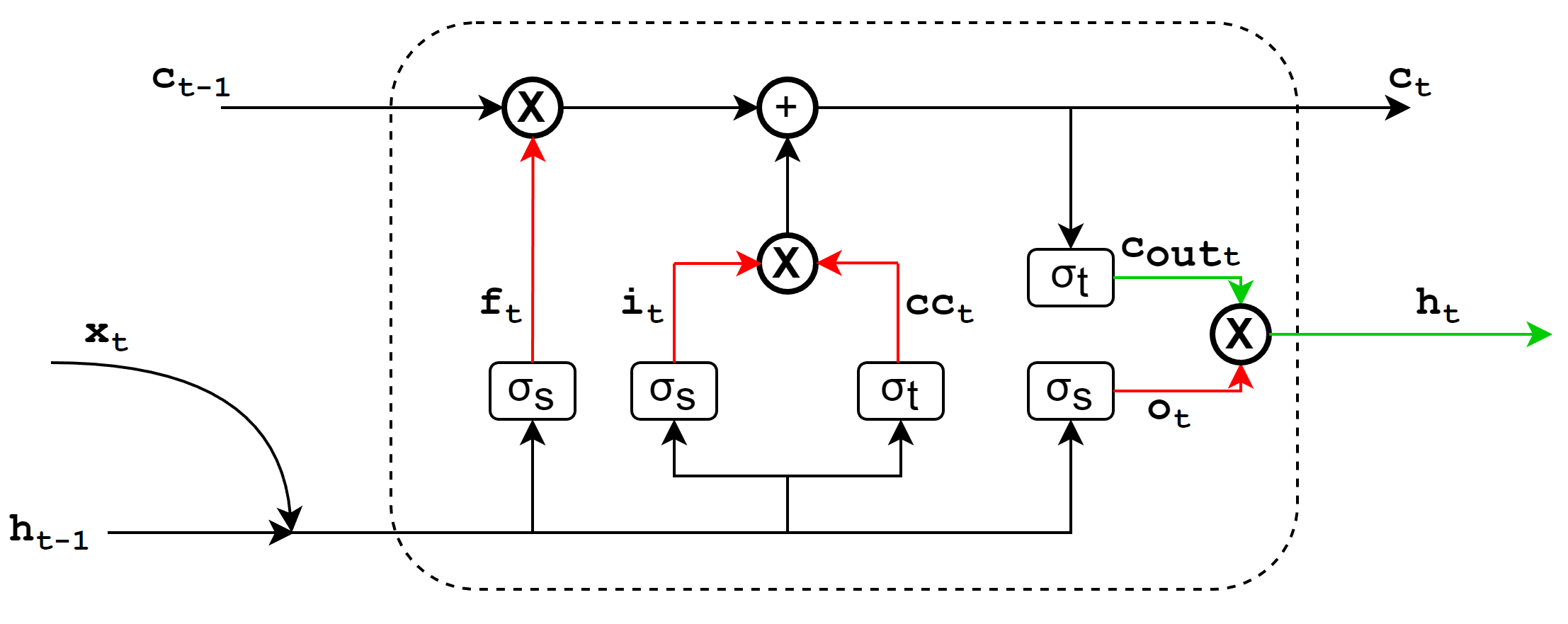
Figure 2: The LSTM cell (dotted circle) with its internal structure shown. The red lines represent the “internal” activations while the green lines represent the “external” activations. $\mathbf{\sigma_{t}}$ and $\mathbf{\sigma_{s}}$ represent the tanh activation and sigmoid activation respectively.

In this study we use a particular type of RNN called Long Short-Term Memory (LSTM) networks. In this arthitecture, an LSTM cell was created to replace the recurrent cell in the vanilla RNN shown in Figure 1 in order to solve the vanishing gradient problem Hochreiter and Schmidhuber (1997). The LSTM network attempts to resolve the problem by maintaining an internal cell state $\mathbf{c}$.

In an LSTM network, the RNN cell shown in Figure 1 is replaced by the LSTM cell (Figure 2) which consists of many different activations compared to the single activation in a vanilla RNN cell. This LSTM cell, like the vanilla RNN cell, takes in $\mathbf{x_{t}}$ and $\mathbf{h_{t-1}}$ as inputs, along with the additional input of the previous cell state $\mathbf{c_{t-1}}$. Like the vanilla RNN, the LSTM cell also outputs the current hidden state $\mathbf{h_{t}}$ and additionally the current cell state $\mathbf{c_{t}}$ to itself in the next timestep. The addition of the internal cell state $\mathbf{c}$ helps in preserving temporal correlations Hochreiter and Schmidhuber (1997).

II Methods

The task selected for this experiment is a popular benchmark AI task, which is to predict the sentiment of natural languages of the Large Movie Review Dataset Maas et al. (2011), which contains 50000 labelled movie reviews from the Internet Movie Database (IMDb). Traditional machine learning techniques like the Naive Bayes classifier, Maximum Entropy (MaxEnt) classification, and Support Vector Machines (SVMs) are effective at topic-based text classification, which classifies text based on keywords. However, they tend to have trouble classifying text based on positive or negative sentiment, which can require a more subtle “understanding” of context beyond single words or short phrases Pang et al. (2002).

LSTM networks have demonstrated long range temporal memory beyond simple n-grams (unit of $n$ words used in traditional natural language processing (NLP) techniques). As such, they are prime candidates for this task and frequently demonstrate close to human level performance in basic sentiment analysis.

In this work we use LSTM rather than other RNN structures due to its superior performance over other variants in real tasks. To analyse specifically the time series behaviour of the LSTM cell activations, the LSTM network used for this task will contain the minimum number of layers to properly classify the data. Additional layers that are traditionally used to augment the performance of the network will not be included as they carry the same key features and do not generate significantly new theoretical insights.

II.1 Dataset

The dataset chosen for the sentiment analysis task will be the Large Movie Review Dataset Maas et al. (2011) which consists of 50000 highly polar movie reviews obtained from the Internet Movie Database (IMDb) . This dataset consists of 25000 positive reviews (score $\geq$ 7 out of 10) and 25000 negative reviews (score $\leq$ 4 out of 10).

Preprocessing steps such as the removal of punctuation and converting of words to lowercase were performed. The words were also converted to tokens, with the top 4000 words (88.3% of the full vocabulary) converted into unique tokens, and the rest of the words converted into a single [UNK] token.

II.2 LSTM network architecture

The LSTM network will consist of three layers: An embedding layer that converts the words into lower dimensional internal representation vectors, the LSTM layer, and an output layer consisting of a single neuron with a sigmoid activation that outputs a value indicating if the review is positive ($y\geq 0.5$) or negative ($y<0.5$).

The IMDb dataset was obtained using the Keras Chollet et al. (2015) datasets application programming interface (API), with the preprocessing done with custom code . The networks were trained using Keras with the TensorFlow 2.6.0 Abadi et al. (2015) backend on a GeForce GTX 1080 GPU, with preprocessing steps performed on a Ryzen 9 3900X CPU.

The hyperparameters used for the LSTM networks are shown in Table 1. These hyperparameters were selected with the KerasTuner O’Malley et al. (2019) library using the Hyperband Li et al. (2017) search algorithm, selected over 10 hyperband iterations. Overall, we follow the best practices of the state-of-the-art for LSTM models in this work.

II.3 Measuring $1/f$ noise

In order to measure the spectral noise in the LSTM cell, temporal sequences of the specific activations have to be obtained. To obtain the internal activations of the Keras LSTM cells, the cell was recreated in vanilla Python with NumPy Harris et al. (2020). The code for this is available at .

The steps to obtain the power spectral density of any specific activation ($\mathbf{f}$ in this case) is then as follows:

1. Propagate the review through the LSTM layer, recording the vector $\mathbf{f}_{t}$ corresponding to the forget gate of each LSTM cell at each timestep $t$, forming 60 time series of activations corresponding to the 60 LSTM cells.

2. Perform a fast Fourier transform (FFT) on each time series.

3. Take the square of the FFT to obtain the PSD of each time series.

4. Sum the activation power spectral density of each cell in the layer to get the total PSD of the LSTM layer .

III Results and Discussion

When picking the optimal epoch of the networks, the epoch with the lowest network loss was selected. The accuracy achieved across the 5 networks was high , ranging from 88.41% to 89.19% prediction accuracy on the test data. Table 2 provides a summary of the network loss and accuracy of the 5 LSTM networks used at the optimal epoch.

Table 2: Summary of the 5 different LSTM network performances on the test dataset of 15000 reviews.

Network	Network loss on test data	Accuracy on test data
1	0.2778	89.19
2	0.2867	88.77
3	0.2896	88.41
4	0.2788	89.07
5	0.2927	88.57

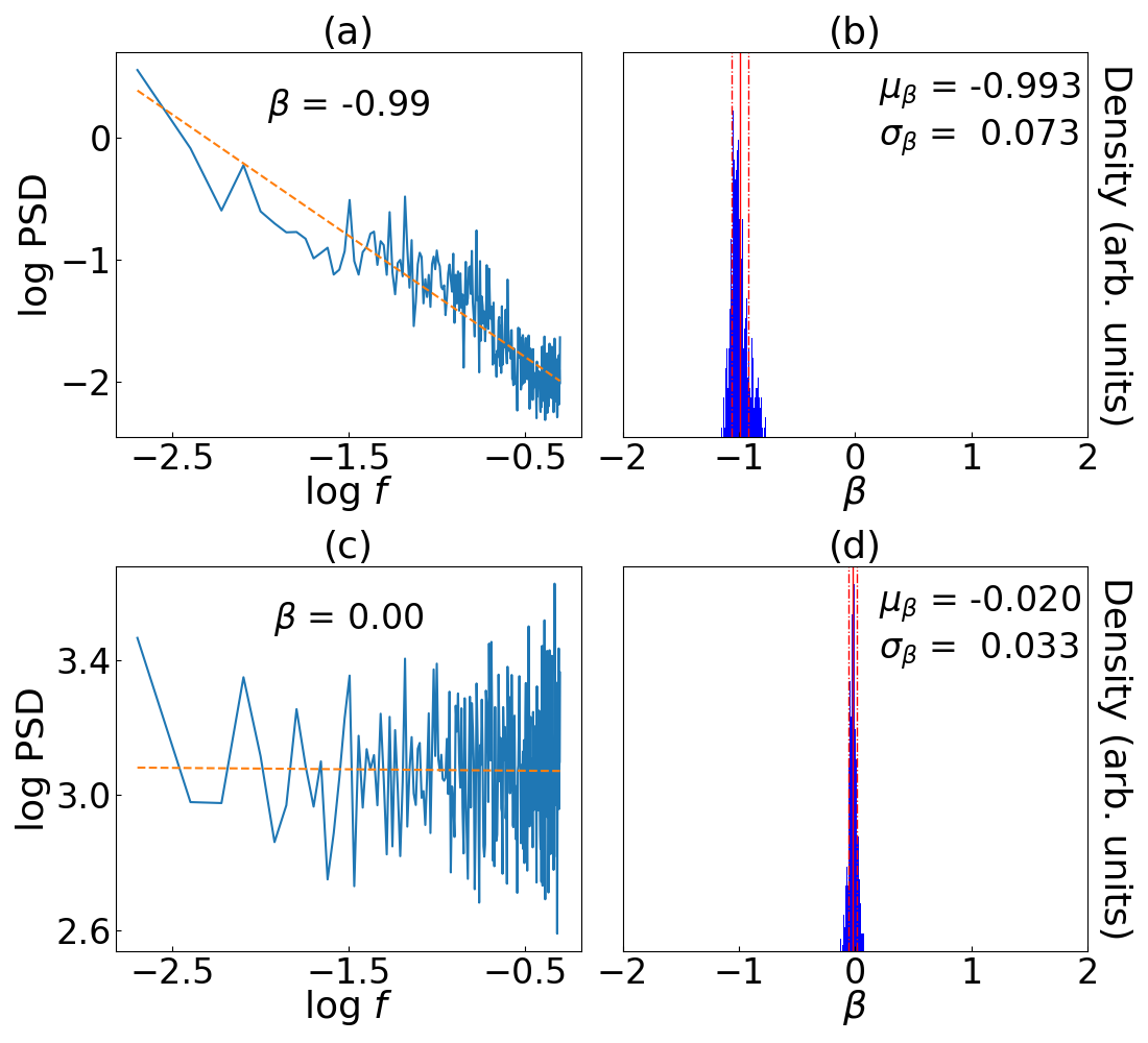
Figure 3: (a) PSD (solid, blue) of the activation $\mathbf{h}_{t}$ for the entire LSTM layer for a single 580 word review (truncated to 500 words) with a line of best fit plotted (dashed, orange). The slope obtained in the log-log plot is the exponent $\beta$, with a value of $\beta=-0.99$. (b) Histogram showing the spread of values of $\beta$ for the activation $\mathbf{h}$ for a single LSTM network across all the test reviews with length $\geq 500$. The mean value (solid, red) $\mu=-0.993$ and standard deviation (dashed, red) $\sigma=0.073$ are indicated on the histogram. (c) PSD (solid, blue) of the input $\mathbf{x}_{t}$ for the same 580 word review shown in (a) with a line of best fit plotted (dashed, orange), giving $\beta=0.00$. (d) Histogram showing the spread of values of $\beta$ for the inputs $\mathbf{x}$ across all the test reviews with length $\geq 500$. The mean value (solid, red) $\mu=-0.020$ and standard deviation (dashed, red) $\sigma=0.033$ are indicated on the histogram.

III.1 Exponent $\beta$ for the test set

The steps described in subsection II.3 were performed for the reviews in the test dataset of length $\geq 500$ to remove the impact of the padding as the repeated identical padding tokens has the effect of lowering the exponent in the PSD. Note that training of the LSTM is carried out on reviews regardless of their word lengths, to keep in line with the accepted practices in AI. Figure 3(a) shows the PSD of one of the reviews for one of the networks, with the exponent for $\mathbf{h}$ obtained by taking the gradient of the PSD on a log-log scale. Figure 3(b) displays a histogram of the exponents of $\mathbf{h}$ obtained for all the test reviews with length $\geq 500$ for the same network. We see clear $1/f$ noise here with a mean $\mu=-0.993\pm 0.073$.

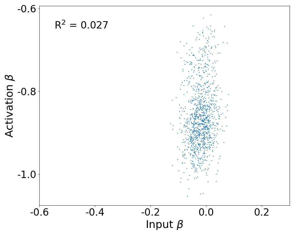
Figure 4: Scatter plot of the exponents of $\mathbf{h}$ vs the exponents of the input $\mathbf{x}$ for test reviews with length $\geq 500$. Model used is the same as Figure 3. The input exponents here are not impacting the activation exponent values, showing that the ‘$1/f$’ phenomenon in the activation values is not from a similar pattern in the inputs.

III.2 Ruling out $1/f$ noise in the input

One possibility for the presence of $1/f$ noise is that the input $\mathbf{x}$ has a PSD that is $1/f$. As such, it is important to rule out this effect if we were to demonstrate the emergence of $1/f$ noise from the LSTM. To determine the exponent of the input data, the same process from II.3 was performed, using the embedding vector instead of the activation vector.

Figure 3(c) shows the PSD of one of the inputs, with the exponent for $\mathbf{x}$ obtained by taking the gradient of the PSD on a log-log scale. Figure 3(d) displays a histogram of the exponents of $\mathbf{x}$ obtained for all the test reviews with length $\geq 500$. Unlike the clear $1/f$ noise demonstrated with the activations from the LSTM layer, the histogram here shows that the noise in the reviews themselves are effectively uncorrelated white noise, with a mean $\mu=-0.020\pm 0.033$.

Figure 4 is a scatter plot relating the histograms shown in Figure 3, demonstrating the lack of correlation between the activation exponent and the input exponent with an $R^{2}$ value of 0.083. This further supports our hypothesis that the $1/f$ noise observed in the LSTM networks are inherent to the networks, rather than a consequence of $1/f$ noise in the inputs to the networks.

Table 3: Summary of exponent $\beta$ values across the 5 LSTM networks before and after training.

Activation	$\beta$ (Untrained)	$\beta$ (Trained)
$\mathbf{f}$	-0.86 $\pm$ 0.31	-0.58 $\pm$ 0.17
$\mathbf{i}$	-0.87 $\pm$ 0.27	-0.62 $\pm$ 0.13
$\mathbf{cc}$	-0.03 $\pm$ 0.29	-0.312 $\pm$ 0.086
$\mathbf{o}$	-0.78 $\pm$ 0.18	-0.56 $\pm$ 0.15
$\mathbf{c_{out}}$	-1.14 $\pm$ 0.31	-1.05 $\pm$ 0.16
$\mathbf{h}$	-1.13 $\pm$ 0.31	-0.80 $\pm$ 0.15

III.3 Overall results for $\beta$

The data for all the activations across all the networks was collected and the aggregate values of $\beta$ for each activation are shown in Table 3. The aggregate values for $\beta$ are provided for the networks before and after training, with the weights of untrained networks randomly initialised with the default GlorotUniform initialiser.

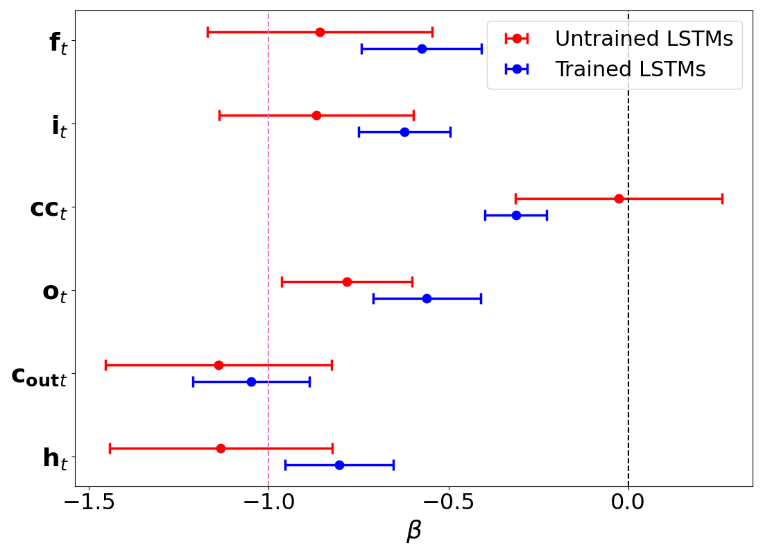
Figure 5: Aggregate values of $\beta$ for all the activations plotted. The error bar represents 1 standard deviation $\sigma$ value over 5 LSTM networks. The dotted pink line marks $\beta=-1.0$ (pink noise), and the dotted black line marks $\beta=0$ (white noise).

The summary of the aggregate results on exponents for different neurons is also shown in Figure 5, where the effect of training is very clearly demonstrated. The “internal” activations $\mathbf{f}$, $\mathbf{i}$, $\mathbf{cc}$, and $\mathbf{o}$ have a relatively less negative trained exponent of between -0.3 and -0.6, while the “external” activations $\mathbf{c_{out}}$ and $\mathbf{h}$ are closer to pink noise, with relatively more negative trained exponents. Another point of interest is that the effect of training is to make the exponents less negative, with the exception of the exponent $\mathbf{cc}$.

This behaviour is similar to that of fMRIs compared to EEGs, where the exponents measured by fMRIs He (2011) corresponding to signals from the volume of the brain are less negative than those measured by EEGs Dehghani et al. (2010) corresponding to signals from the surface of the brain.

III.4 Effect of performing a task on $\beta$

It has been reported that the exponent $\beta$ from human brain exhibits different values when at rest and performing tasks. Specifically, its value is more negative when at rest as compared to the latterHe (2011). Here we also mimic the ‘rest’ state and ‘task’ state of the LSTM: we assume that using inputs consisting of only 0 values mimics the ‘rest’ state, and using inputs of actual movie reviews mimics the ‘task’ state. As shown from the results in Figure 6, intriguingly the LSTM exhibits the same trend in the value of $\beta$: it is more negative when at ‘rest’. One possible explanation is that a more negative $\beta$ value is associated with a longer memory process. And since the ‘rest’ state has constant values as input, this input data naturally has longer memory than that of the ‘task’ inputs. This longer memory process then gets carried over to the outputs of the neural network values.

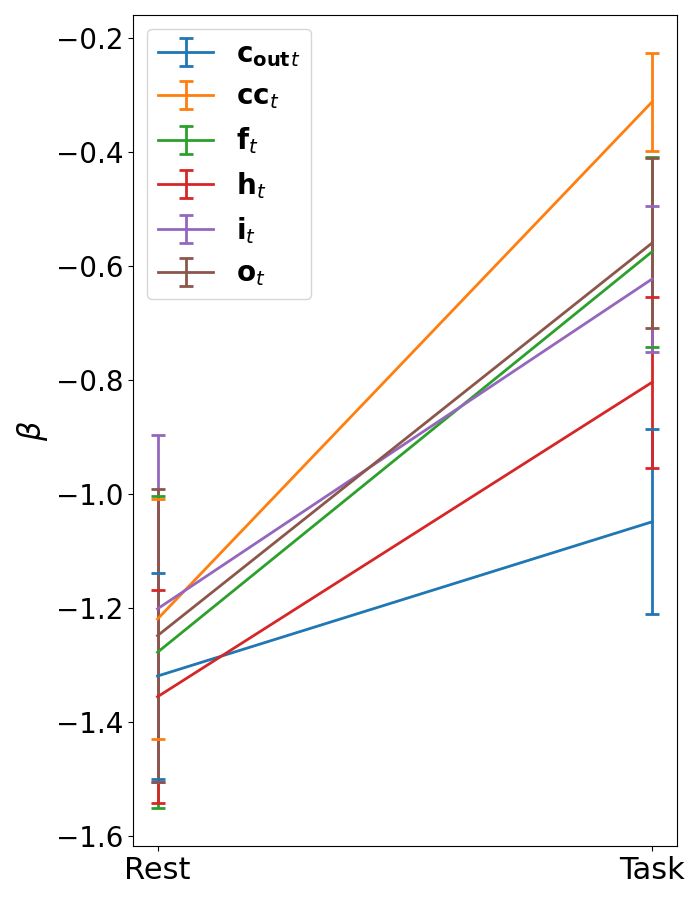
Figure 6: The effect of performing a task on the exponent $\beta$ of the various activations in the LSTM networks. This is drawn in direct analogy with the “rest” vs. “task” measurements for fMRI signals in human subjects He (2011). The exponents obtained for “task” correspond to the LSTM cells processing input vectors that correspond to movie reviews. The exponents obtained for “rest” correspond to the LSTM cells processing zero vectors of equal dimension to the movie reviews (40 dimensions after the embedding layer) for 500 timesteps.

IV Conclusion

In summary, we have found that $1/f$ noise is also present in artificial neural networks like the Long Short Term Memory networks that are trained on a real world dataset. Further analysis showed that such a pattern is not a trivial consequence of a similar pattern in input data, as the input data shows a clear white noise pattern that is distinct from pink noise a.k.a. $1/f$ noise. Since the input data are also real world natural language sentences that our brain processes, our results demonstrates that artificial network networks that perform close to the cognition of human level exhibits very similar $1/f$ patterns as the later biological counterpartsNovikov et al. (1997); He (2014, 2011). The analogy was also further extended with the similarity of the trends in the noise exponents for “inner” and “outer” neurons within the LSTM compared to fMRI and EEG exponents respectively Dehghani et al. (2010); He (2011). Similarly, the noise exponents for the LSTM networks at “rest” state compared to when performing the tasks exhibit the same trend found in fMRI data He (2011).

It is intriguing that despite the vast differences in the microscopic details between biological neural networks and artificial neural networks, such macroscopic patterns of $1/f$ are strikingly similar. Such similarity points at some deeper principles that govern their healthy functioning, something that is independent of the detailed neural interactions. With the artificial neural networks being more ‘transparent’ to our experimental manipulation and examination unlike its biological counterpart, it is an ideal proxy to understand the origin of $1/f$ noise going forward, as well as a possible tool to understand more about the healthy functioning of the brain through the $1/f$ noise perspective.

References

- Åström (1970) K. J. Åström, “Stochastic Processes,” in Introduction to Stochastic Control Theory, Mathematics in Science and Engineering, Vol. 70 (Elsevier, 1970) pp. 13–43.
- Bass (2011) R. F. Bass, “Brownian motion,” in Stochastic Processes, Cambridge Series in Statistical and Probabilistic Mathematics (Cambridge University Press, 2011) p. 6–12.
- Hooge and Gaal (1971) F. N. Hooge and J. L. M. Gaal, Philips Res. Rep 26, 77 (1971).
- van der Ziel (1970) A. van der Ziel, Proceedings of the IEEE 58, 1178 (1970).
- Fu and Sah (1972) H.-S. Fu and C.-T. Sah, IEEE Transactions on Electron Devices 19, 273 (1972).
- Mück et al. (2005) M. Mück, M. Korn, C. G. A. Mugford, J. B. Kycia, and J. Clarke, Applied Physics Letters 86, 012510 (2005).
- Taft et al. (1974) B. A. Taft, B. M. Hickey, C. Wunsch, and D. J. Baker Jr., “Equatorial undercurrent and deeper flows in the central Pacific,” (Elsevier, 1974) pp. 403–430.
- Moon et al. (2018) W. Moon, S. Agarwal, and J. S. Wettlaufer, Physical Review Letters 121, 108701 (2018).
- Mandelbrot and Wallis (1968) B. B. Mandelbrot and J. R. Wallis, Water Resources Research 4, 909 (1968).
- Mandelbrot and Wallis (1969) B. B. Mandelbrot and J. R. Wallis, Water Resources Research 5, 321 (1969).
- Musha and Higuchi (1978) T. Musha and H. Higuchi, Japanese Journal of Applied Physics 17, 811 (1978).
- Nagatani (1993) T. Nagatani, Journal of the Physical Society of Japan 62, 2533 (1993).
- Carpinteri et al. (2018) A. Carpinteri, G. Lacidogna, and F. Accornero, Applied Sciences 8 (2018), 10.3390/app8091685.
- Voss and Clarke (1978) R. F. Voss and J. Clarke, The Journal of the Acoustical Society of America 63, 258 (1978).
- Peng et al. (1993) C.-K. Peng, J. Mietus, J. M. Hausdorff, S. Havlin, H. E. Stanley, and A. L. Goldberger, Physical Review Letters 70, 1343 (1993).
- Struzik et al. (2004) Z. R. Struzik, J. Hayano, S. Sakata, S. Kwak, and Y. Yamamoto, Physical Review E 70, 050901 (2004).
- Musha et al. (1981) T. Musha, Y. Kosugi, G. Matsumoto, and M. Suzuki, IEEE Transactions on Biomedical Engineering BME-28, 616 (1981).
- Medina and Díaz (2012) J. M. Medina and J. A. Díaz, J. Opt. Soc. Am. A 29, A82 (2012).
- Novikov et al. (1997) E. Novikov, A. Novikov, D. Shannahoff-Khalsa, B. Schwartz, and J. Wright, Physical Review E 56, R2387 (1997).
- Schottky (1926) W. Schottky, Phys. Rev. 28, 74 (1926).
- Christensen and Pearson (1936) C. J. Christensen and G. L. Pearson, The Bell System Technical Journal 15, 197 (1936).
- Zinn-Justin (2002) J. Zinn-Justin, Quantum Field Theory and Critical Phenomena (Oxford Science Publications, 2002).
- Ódor (2004) G. Ódor, Reviews of Modern Physics 76, 663 (2004).
- Creswick and Kim (1997) R. J. Creswick and S.-Y. Kim, Journal of Physics A: Mathematical and General 30, 8785 (1997).
- Aggarwal (2018) C. C. Aggarwal, Neural Networks and Deep Learning (Springer, 2018).
- He (2014) B. J. He, Trends in Cognitive Sciences 18, 480 (2014).
- Racz et al. (2021) F. S. Racz, K. Farkas, O. Stylianou, Z. Kaposzta, A. Czoch, P. Mukli, G. Csukly, and A. Eke, Brain and Behavior 11, e02047 (2021).
- He et al. (2010) B. J. He, J. M. Zempel, A. Z. Snyder, and M. E. Raichle, Neuron 66, 353 (2010).
- Niedermeyer (2017) E. Niedermeyer, Electroencephalography: Basic Principles, Clinical Applications, and Related Fields, 7th ed., edited by D. L. Schomer and F. H. Lopes da Silva (Oxford University Press, 2017).
- Dehghani et al. (2010) N. Dehghani, C. Bédard, S. Cash, E. Halgren, and A. Destexhe, Journal of Computational Neuroscience 29, 405 (2010).
- Pathania et al. (2021) A. Pathania, M. Schreiber, M. W. Miller, M. J. Euler, and K. R. Lohse, International Journal of Psychophysiology 160, 18 (2021).
- Huettel et al. (2008) S. A. Huettel, A. W. Song, and G. McCarthy, Functional Magnetic Resonance Imaging, 2nd ed. (Sinauer Associates, Inc., 2008).
- Logothetis et al. (2001) N. K. Logothetis, J. Pauls, M. Augath, T. Trinath, and A. Oeltermann, Nature 412, 150 (2001).
- He (2011) B. J. He, Journal of Neuroscience 31, 13786 (2011).
- Hochreiter and Schmidhuber (1997) S. Hochreiter and J. Schmidhuber, Neural Computation 9 (1997), 10.1162/neco.1997.9.8.1735.
- Maas et al. (2011) A. L. Maas, R. E. Daly, P. T. Pham, D. Huang, A. Y. Ng, and C. Potts, in Proceedings of the 49th Annual Meeting of the Association for Computational Linguistics: Human Language Technologies (Association for Computational Linguistics, Portland, Oregon, USA, 2011) pp. 142–150.
- Pang et al. (2002) B. Pang, L. Lee, and S. Vaithyanathan, in Proceedings of EMNLP (2002) pp. 79–86.
- Note (1) Https://www.imdb.com/.
- Chollet et al. (2015) F. Chollet et al., “Keras,” https://keras.io (2015).
- Note (2) https://github.com/NicholasCJL/imdb-LSTM/blob/master/data_processing.py.
- Abadi et al. (2015) M. Abadi, A. Agarwal, P. Barham, E. Brevdo, Z. Chen, C. Citro, G. S. Corrado, A. Davis, J. Dean, M. Devin, S. Ghemawat, I. Goodfellow, A. Harp, G. Irving, M. Isard, Y. Jia, R. Jozefowicz, L. Kaiser, M. Kudlur, J. Levenberg, D. Mané, R. Monga, S. Moore, D. Murray, C. Olah, M. Schuster, J. Shlens, B. Steiner, I. Sutskever, K. Talwar, P. Tucker, V. Vanhoucke, V. Vasudevan, F. Viégas, O. Vinyals, P. Warden, M. Wattenberg, M. Wicke, Y. Yu, and X. Zheng, “TensorFlow: Large-scale machine learning on heterogeneous systems,” (2015), software available from tensorflow.org.
- O’Malley et al. (2019) T. O’Malley, E. Bursztein, J. Long, F. Chollet, H. Jin, L. Invernizzi, et al., “Keras Tuner,” https://github.com/keras-team/keras-tuner (2019).
- Li et al. (2017) L. Li, K. Jamieson, G. DeSalvo, A. Rostamizadeh, and A. Talwalkar, Journal of Machine Learning Research 18, 6765–6816 (2017).
- Harris et al. (2020) C. R. Harris, K. J. Millman, S. J. van der Walt, R. Gommers, P. Virtanen, D. Cournapeau, E. Wieser, J. Taylor, S. Berg, N. J. Smith, R. Kern, M. Picus, S. Hoyer, M. H. van Kerkwijk, M. Brett, A. Haldane, J. F. del Río, M. Wiebe, P. Peterson, P. Gérard-Marchant, K. Sheppard, T. Reddy, W. Weckesser, H. Abbasi, C. Gohlke, and T. E. Oliphant, Nature 585, 357 (2020).
- Note (3) https://github.com/NicholasCJL/imdb-LSTM/blob/master/get_LSTM_internal_vectorized.py.
- Note (4) It has been found experimentally in the course of this work that calculating the cell-level PSD before summing to get the layer PSD gives very similar exponents compared to summing the cell-level signals to get the overall layer signal before calculating the PSD of that signal.
- Note (5) For reference, the best-performing LSTM based classifier has a 94.1% accuracy, and the best-performing model is a transformer with 96.1% accuracy. Taken from https://paperswithcode.com/sota/sentiment-analysis-on-imdb.