MAMMOTH-Subaru III. Ly$\alpha$ Halo Extended to $\sim 200$ kpc Identified by Stacking $\sim 3300$ Ly$\alpha$ Emitters at $z=2.2-2.3$

Abstract

In this paper, we present a Ly$\alpha$ halo extended to $\sim 200$ kpc identified by stacking $\sim 3300$ Ly$\alpha$ emitters at $z=2.2-2.3$. We carry out imaging observations and data reduction with Subaru/Hyper Suprime-Cam (HSC). Our total survey area is $\sim 12$ deg² and imaging depths are $25.5-27.0$ mag. Using the imaging data, we select 1,240 and 2,101 LAE candidates at $z=2.2$ and 2.3, respectively. We carry out spectroscopic observations of our LAE candidates and data reduction with Magellan/IMACS to estimate the contamination rate of our LAE candidates. We find that the contamination rate of our sample is low (8%). We stack our LAE candidates with a median stacking method to identify the Ly$\alpha$ halo at $z=2$. We show that the Ly$\alpha$ halo is extended to $\sim 200$ kpc at a surface brightness level of $10^{-20}$ erg s^-1 cm^-2 arcsec^-2. Comparing to previous studies, our Ly$\alpha$ halo is more extended at radii of $\sim 25-100$ kpc, which is not likely caused by the contamination in our sample but by different redshifts and fields instead. To investigate how central galaxies affect surrounding LAHs, we divide our LAEs into subsamples based on the Ly$\alpha$ luminosity ($L_{\rm Ly\alpha}$), rest-frame Ly$\alpha$ equivalent width (EW₀), and UV magnitude (M_uv). We stack the subsamples and find that higher $L_{\rm Ly\alpha}$, lower EW₀, and brighter M_uv cause more extended halos. Our results suggest that more massive LAEs generally have more extended Ly$\alpha$ halos.

1 Introduction

In the last two decades, diffuse and faint Ly$\alpha$ emission known as Ly$\alpha$ halos (LAHs) are found ubiquitously around Ly$\alpha$ emitters (LAEs) at $z\sim 2-7$ (e.g. Hayashino et al. 2004; Rauch et al. 2008; Steidel et al. 2011; Matsuda et al. 2012; Feldmeier et al. 2013; Momose et al. 2014, 2016; Wisotzki et al. 2016, 2018; Xue et al. 2017; Leclercq et al. 2017; Cai et al. 2019; Kakuma et al. 2021; Lujan Niemeyer et al. 2022; Kikuchihara et al. 2022). Some LAHs are identified by stacking a large number of LAEs to increase the signal-to-noise ratio (e.g. Momose et al. 2014, Wisotzki et al. 2018, and Lujan Niemeyer et al. 2022), while the other LAHs are detected individually by deep integral-field-unit (IFU) observations (e.g. Wisotzki et al. 2016 and Leclercq et al. 2017.) LAHs are believed to trace hydrogen gas in the circumgalactic medium (CGM), and the CGM is related to the central galaxy via processes such as inflow, outflow, and radiation (e.g. Dekel et al. 2009; Sadoun et al. 2019). Thus, LAH is an important population to understand how CGM affects galaxy formation and evolution.

Until recent years, LAHs are only identified at radii smaller than $\sim 100$ kpc due to the limited depths (e.g. Momose et al. 2014; Xue et al. 2017; Arrigoni Battaia et al. 2019; Cai et al. 2019). Kakuma et al. (2021) and Kikuchihara et al. (2022) greatly update the record and find that LAHs are possibly extended to $\sim 1000$ kpc, although the radius bin sizes are not small enough to investigate the transition from central galaxy to CGM (several kpc to several hundred kpc). On the other hand, Lujan Niemeyer et al. (2022) use relatively small radius bin sizes and identify a LAH extended to 320 kpc at $z=1.9-3.5$, although there are only two bins at radii $\gtrsim 100$ kpc ($80-160$ and $160-320$ kpc).

After identification of LAHs, previous studies have investigated how central galaxies affect LAHs. Momose et al. (2016) find that galaxies with a lower Ly$\alpha$ luminosity ($L_{\rm Ly\alpha}$), lower rest-frame Ly$\alpha$ equivalent width (EW₀), and brighter UV magnitude (M_uv) have more extended halos. On the contrary, Xue et al. (2017) and Lujan Niemeyer et al. (2022) find that galaxies with higher $L_{\rm Ly\alpha}$ show more extended halos. The reason causing contradictory results is still not clear.

In this paper, we present a LAH extended to $\sim 200$ kpc identified by stacking $\sim 3300$ Ly$\alpha$ emitters at $z=2$. This paper is structured as follows. We introduce our imaging observations and data reduction in Section 2. The sample selection is presented in Section 3. Section 4 shows our spectroscopic observations, data reduction, and contamination rate estimation. Our results and discussion are presented in Section 5. Finally we summarize this paper in Section 6.

Throughout this paper, we use AB magnitudes (Oke & Gunn, 1983) and physical distances. A $\Lambda$CDM cosmology with $\Omega_{m}=0.3$, $\Omega_{\Lambda}=0.7$, and $h=0.7$ is adopted.

2 Imaging Observations and Data Reduction

We carry out narrowband (NB) and broadband (BB) imaging observations with Subaru/Hyper Suprime-Cam (HSC; Miyazaki et al. 2018; Komiyama et al. 2018; Kawanomoto et al. 2018; Furusawa et al. 2018). The narrowband filters we use are NB387 ($\lambda_{\mathrm{c}}=3863$ Å, FWHM=55 Å) and NB400 ($\lambda_{\mathrm{c}}=4003$ Å, FWHM=92 Å), and the broadband is $g$ ($\lambda_{\mathrm{c}}=4754$ Å, FWHM=1395 Å). The central wavelengths of NB387 and NB400 filters are chosen to detect redshifted Ly$\alpha$ emission at $z=2.2$ and $2.3$, respectively. More details of the observations are described in Liang et al. (2021) and Liang et al. (in prep.). In brief, we observe four fields (J0210, J0222, J0924, and J1419) with NB387 and four other fields (J0240, J0755, J1133, and J1349) with NB400 between January 2018 and March 2020. The detailed field selection are described in Cai et al. (2016), Liang et al. (2021), Cai et al. (in prep.), and Liang et al. (in prep.). The seeing sizes are $0.7-1.2$ arcsec depending on the fields, with smallest seeing in J1419 and largest seeing in J0210. The total survey area is $\sim 12$ deg².

The imaging data are reduced with the HSC pipeline dubbed hscPipe (Bosch et al. 2018; Aihara et al. 2018). The NB387 and $g$ images of four NB387 fields are reduced by Liang et al. (2021). We reduce the NB400 and $g$ images of the four NB400 fields in the same manner as Liang et al. (2021). In brief, we first carry out bias subtraction, dark subtraction, flat-field calibration, and stacking of individual exposures. We then use the imaging data from the Panoramic Survey Telescope and Rapid Response System 1 (Pan-STARRS1; Schlafly et al. 2012; Tonry et al. 2012; Magnier et al. 2013) survey to calibrate the astrometry and photometry with sky subtraction. The $5\sigma$ detection limits of the final imaging products are $24.3-25.0$, $25.5-25.8$, and $26.2-27.0$ mag for NB387, NB400, and $g$, respectively. The above detection limits are measured in a $1^{\prime\prime}.7$ diameter aperture, except for J0210 field in a $2^{\prime\prime}.5$ diameter aperture. Details of the fields are summarized in Table 1.

We carry out source detection and photometry with SExtractor (Bertin & Arnouts, 1996) to build our source catalogs. The source catalogs of four NB387 fields are obtained by Liang et al. (2021), and we make the source catalogs of the four NB400 fields in the same manner. Firstly, we convolve the NB400 and $g$ images with proper Gaussian kernels to match the point-spread-functions (PSFs) of NB and BB filters. Then, we use the NB400 images as the reference images to detect sources in the dual-image mode of SExtractor. The detection criterion is 15 adjacent pixels above the $1.2\sigma$ limit. To reduce the effect of different depths across the field, we use the sky background root-mean square map as the weight image. The mesh size used for sky background estimation is 128 pixels. We do not use regions with low signal-to-noise ratios (SNRs) or bad pixels such as field edges and bright star vicinity.

Table 1: Information of fields in this study

Field	R.A. (J2000)	Decl. (J2000)	Obs. Date	Filters	$m_{\mathrm{NB},5\sigma}$	$m_{\mathrm{BB},5\sigma}$	$N_{\rm LAE}$
name	hh:mm:ss	dd:mm:ss	month,year	name	mag	mag	count
J0210	02:09:58.90	+00:53:43.0	Jan., 2018	NB387 & $g$	24.25	26.34	227
J0222	02:22:24.66	-02:23:41.2	Jan., 2018	NB387 & $g$	24.99	27.01	422
J0924	09:24:00.70	+15:04:16.7	Jan. & Mar., 2019	NB387 & $g$	24.74	26.63	311
J1419	14:19:33.80	+05:00:17.2	Mar., 2019	NB387 & $g$	24.81	26.80	280
J0240	02:40:05.11	-05:21:06.7	Nov., 2019	NB400 & $g$	25.61	26.80	517
J0755	07:55:35.89	+31:09:56.9	Nov., 2019	NB400 & $g$	25.83	26.50	545
J1133	11:33:02.40	+10:05:06.0	Mar., 2020	NB400 & $g$	25.49	26.30	403
J1349	13:49:40.80	+24:28:48.0	Mar., 2020	NB400 & $g$	25.67	26.15	636

Note. — Column 1: field name; Column 2: right ascension; Column 3: declination; Column 4: date of observation; Column 5: filters used; Column 6: 5$\sigma$ limiting magnitude of narrowband; Column 7: 5$\sigma$ limiting magnitude of broadband; Column 8: number of LAE candidates selected in this study.

3 Sample Selection

Using the reduced images and source catalogs, we select LAEs by an excess of the narrowband minus broadband (NB-BB) color in a manner similar to previous studies (e.g. Konno et al. 2016; Liang et al. 2021). Our NB387 LAE selection is based on the LAE catalogs in Liang et al. (2021), but we apply more strict criteria to mainly reduce spurious faint sources. Our selection criteria for NB387 LAEs are:

$$\begin{gathered}g_{\rm ap}-NB387_{\rm ap}>0.3\ \mathrm{and}\ g_{\rm tot}-NB387_{\rm tot}>0.3\ \mathrm{and}\\ g_{\rm ap}-NB387_{\rm ap}>(g_{\rm ap}-NB387_{\rm ap})^{3\sigma}\ \mathrm{and}\\ g_{\rm tot}-NB387_{\rm tot}>(g_{\rm tot}-NB387_{\rm tot})^{3\sigma}\ \mathrm{and}\\ 20.5<NB387_{\rm ap}<NB387^{5\sigma},\end{gathered}$$ (1)

where the subscripts “ap” and “tot” mean the aperture and total magnitudes, respectively. We use the “AUTO” magnitude in SExtrator as the total magnitude. The superscripts “$3\sigma$” and “$5\sigma$” represent the $3\sigma$ and $5\sigma$ limits, respectively. If the $g$ magnitude of a source is fainter than the $2\sigma$ limit, we use the $2\sigma$ limit instead. The $(g-NB387)^{3\sigma}$ is the $3\sigma$ color error that is calculated by $(g-NB387)^{3\sigma}=-2.5\log(1\pm 3\sqrt{f_{\rm{err},g}^{2}+f_{\rm{err},\rm{NB387}}^{2}}/f_{\rm NB387})$, where $f_{\rm{err},g}$ and $f_{\rm{err},\rm{NB387}}$ are the $1\sigma$ errors in $g$ and NB387, respectively. The NB-BB color limit ($>0.3$) corresponds to a rest-frame Ly$\alpha$ equivalent width of $>20$Å. After applying the above criteria, we carry out visual inspection to remove spurious sources such as cosmic rays and satellite trails. After visual inspection, the final number of our NB387 LAE candidates is 1240.

We select NB400 LAEs in the same manner as NB387 LAEs. As shown in Figure 1, our selection criteria for NB400 LAEs are:

$$\begin{gathered}g_{\rm ap}-NB400_{\rm ap}>0.4\ \mathrm{and}\ g_{\rm tot}-NB400_{\rm tot}>0.4\ \mathrm{and}\\ g_{\rm ap}-NB400_{\rm ap}>(g_{\rm ap}-NB400_{\rm ap})^{3\sigma}\ \mathrm{and}\\ g_{\rm tot}-NB400_{\rm tot}>(g_{\rm tot}-NB400_{\rm tot})^{3\sigma}\ \mathrm{and}\\ 18.0<NB400_{\rm ap}<NB387^{5\sigma},\end{gathered}$$ (2)

where the meaning of symbols is the same as Equation 1. After visual inspection, the final number of our NB400 LAE candidates is 2101.

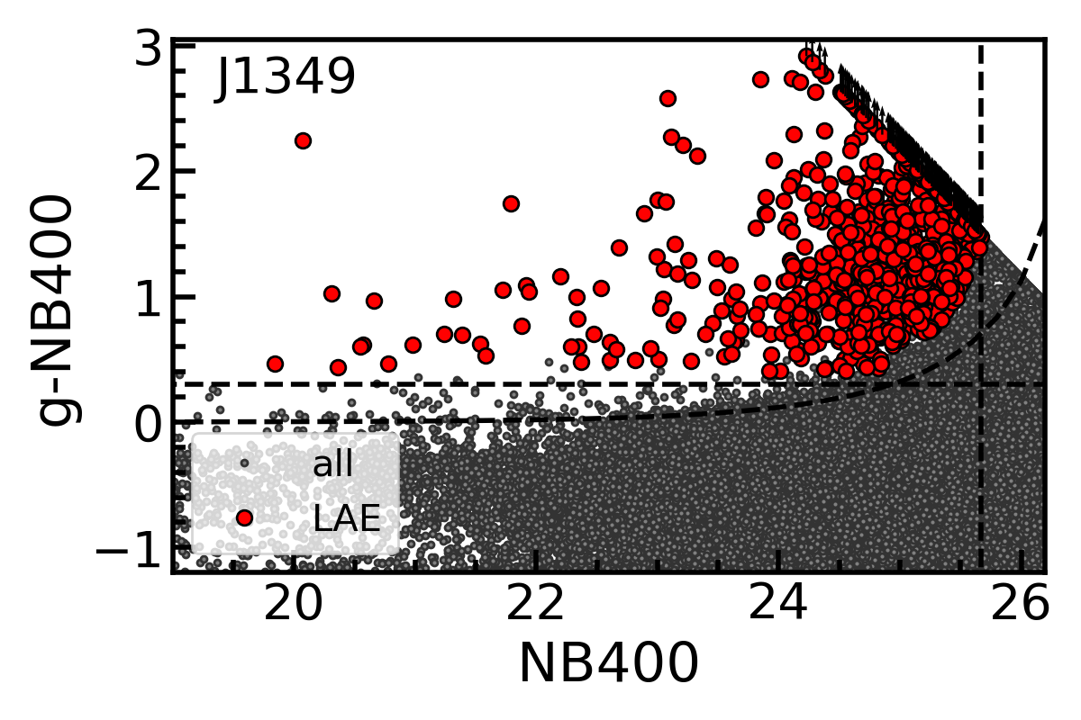
Figure 1: Color-magnitude diagram of NB400 LAE candidates (red) and all detected sources in the source catalog (black). The all detected sources include contamination such as foreground objects, cosmic rays, and satellite trails. The dashed lines represent our selection criteria. This figure shows the LAE selection in the J1349 field as an example. There is a sequence of LAE candidates with black arrows in the upper right corner. This is because that if the $g$ magnitude of a source is fainter than the $2\sigma$ limit, we use the $2\sigma$ limit instead.

4 Contamination Rate Estimation

4.1 Spectroscopic Observations and Data Reduction

To estimate the contamination rate of our NB387 and NB400 LAE candidates, we carry out spectroscopic observations with Magellan/IMACS on September 29 and 30, 2022. The Magellan/IMACS is set in the multislit spectroscopy mode with the f/2 camera, which provides a field of view of $12^{\prime\prime}$ in circular radius. We use the 400 lines per mm grism combined with a filter to cover the wavelength between $\sim 3600$ and 5700 Å. The spectral resolution is $\sim 7$Å using this setup with a slit width of 1.2 arcsec and slit length of 8.0 arcsec. We observe one pointing in each of J0210 and J0222 fields for NB387 LAEs, and 2 pointings in the J0240 field for NB400 LAEs. The on-source exposure times are 7500s and 6000s for NB387 and NB400 LAEs, respectively.

We reduce the spectroscopic data using the official pipeline named COSMOS. We carry out bias subtraction, flat calibration, wavelength calibration, sky subtraction, two-dimensional spectrum extraction, and stacking of individual exposures. We use dome flat frames for the flat calibration, and Helium-Mercury lamp spectra for the wavelength calibration. We do not conduct flux calibration yet, because it is not necessary for the purpose of contamination rate estimation.

4.2 Contamination Rate Calculation

After the data reduction, we obtain 120 and 151 spectra for NB387 and NB400 LAEs, respectively. Among the total 271 spectra, there are 120 spectra with a detected emission line at the expected wavelengths of Ly$\alpha$. The detection fraction is not high because that the real on-source exposure time is shorter than expected. Another reason is that we also observe low-priority faint LAE candidates as the available slits on a slit mask are much more than our high-priority bright targets. Among the 120 spectra with detection, 22 spectra are confirmed LAEs at $z=2$ with $\geq 2$ emission lines, and 2 spectra are foreground objects with $\geq 2$ emission lines. The 22 LAEs with $\geq 2$ emission lines are typically detected in Ly$\alpha$, C iv, and/or He ii. The 2 foreground objects with $\geq 2$ emission lines include a C iv+C iii emitter at $z=1.711$ and a C iv+He ii+C iii emitter at $z=1.793$. Because our spectral resolution ($\sim 7$Å) is not high enough to resolve the doublet of a foreground [O ii] emitter, we only use the spectra with $\geq 2$ emission lines when estimating the contamination rate. The contamination rate of our LAE candidates is thus 2/(22+2)$\approx$8%. The NB magnitudes of the 24 objects with $\geq 2$ emission lines are 21.3-25.3 mag.

5 Results and Discussion

5.1 LAE Stacking

After obtaining our LAE catalogs, we stack the NB387 and NB400 LAE candidates to detect the faint and extended Ly$\alpha$ halo at $z=2$. First, we match PSFs of all filters (NB387, NB400, and $g$) in all the 8 fields by convolution with proper Gaussian kernels. Then we make cutout narrowband (NB387 or NB400) and broadband ($g$) images with a size of $84^{\prime\prime}\times 84^{\prime\prime}$ for each LAE. During this process, we remove six NB387 LAEs because they are too close to the field edges and we cannot make their cutout images with the $84^{\prime\prime}\times 84^{\prime\prime}$ size. We subtract the narrowband images by broadband images to obtain Ly$\alpha$ images. We stack the Ly$\alpha$ images with a median stacking method for NB387 and NB400 LAEs separately. Because the expected redshifts of NB387 and NB400 LAEs are very close ($\Delta z\sim 0.1$), we also stack NB387 and NB400 LAEs together and this is referred to as the all sample in the following sections. The number of LAEs used for stacking are 1234, 2101, and 3335 for the NB387, NB400, and all LAEs, respectively. It should be noted that the 3335 all LAEs contain 117 Ly$\alpha$ blobs (LABs) whose details are described in Li et al. (in prep.) and Zhang et al. (in prep.). We do not remove these LABs during the stacking, because there are no evidences showing that extended Ly$\alpha$ emission of LABs is generally distinct (Zhang et al. 2020). After stacking, we globally subtract the median value measured in a radius of $34^{\prime\prime}-42^{\prime\prime}$ ($\sim 280-350$ kpc) from the image to remove the small sky residual or sky over-subtraction.

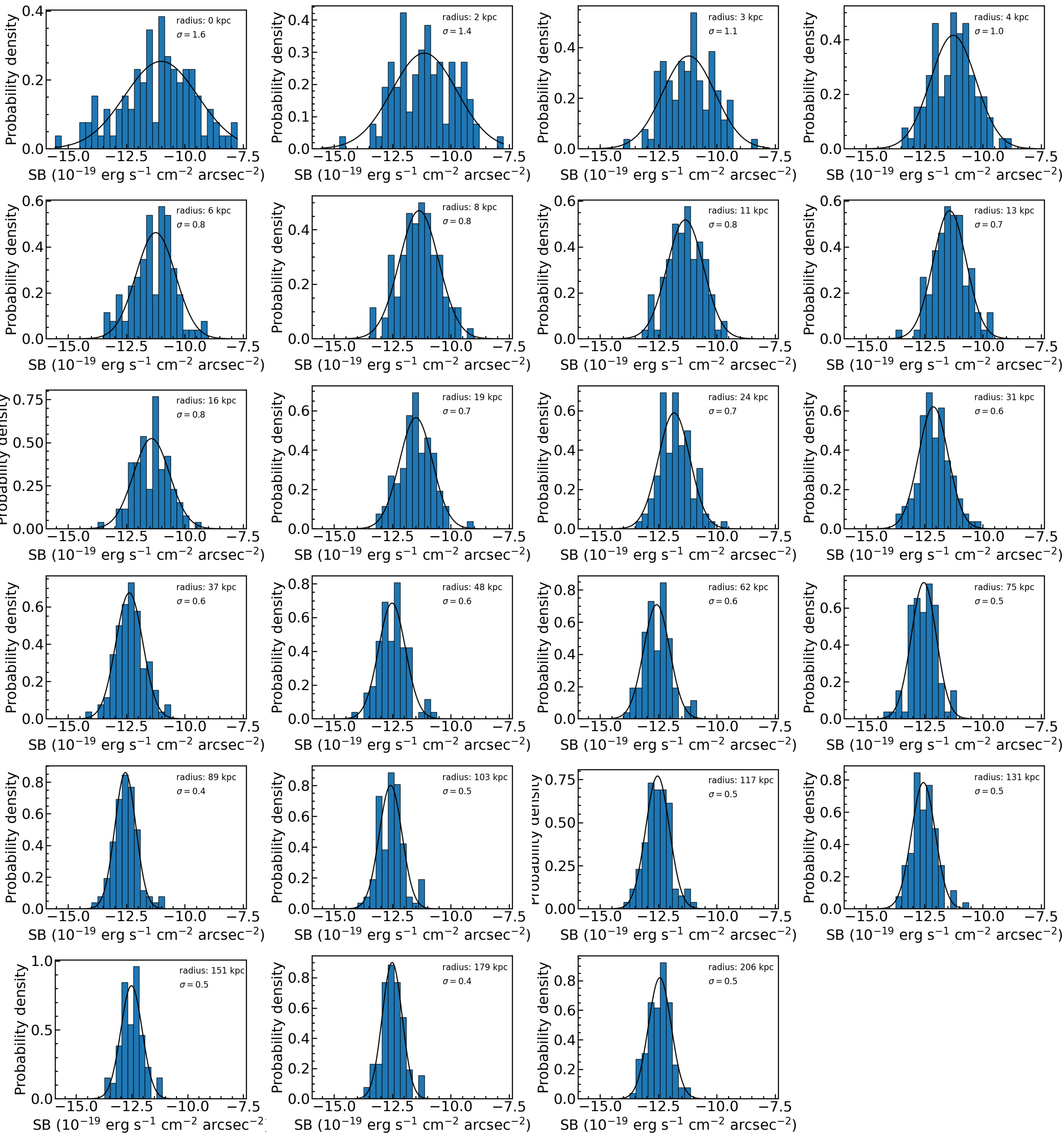
Figure 7: Histograms of the surface brightness distribution of sky in each radius bin. The radius of each bin is indicated in each panel. The black solid line shows the best-fit Gaussian function. The $\sigma$ of the best-fit Gaussian function is shown in each panel in a unit of $10^{-19}$ erg s^-1 cm^-2 arcsec^-2. The values of $\sigma$ are equal to the vertical error bars of black points in Figures 3, 4, 5, and 6.

We estimate the uncertainty of our stacking results by the following method. Firstly, we randomly choose sky regions and make cutout sky images with the same number as our LAE samples. The sky region means that a region with no detected objects within a radius of 20 pixels ($3^{\prime\prime}.4$) from the center. This is because when we visually inspect LAEs in Section 3, we only remove LAE candidates contaminated by close (separation $\lesssim 3^{\prime\prime}$) non-LAE objects. As a result, it is natural that far (separation $\gtrsim 3^{\prime\prime}$) contaminants exist around our LAEs. Then we stack the sky images in the same manner as our LAEs. We repeat the above procedures for 100 times and obtain 100 stacked sky images. Finally we plot histograms of surface brightness using the stacked sky images and fit a Gaussian function to measure the 1$\sigma$ uncertainties at different radii. We find that the 1$\sigma$ uncertainties at radii of $\gtrsim 75$ kpc are between $4\times 10^{-20}$ and $5\times 10^{-20}$ erg s^-1 cm^-2 arcsec^-2. The surface brightness distributions of sky at different radii are shown in Figure 7 in Appendix.

Figure 2 shows our stacked Ly$\alpha$ images and Figure 3 shows the Ly$\alpha$ surface brightness profiles. Clearly, the Ly$\alpha$ emission is extended to $\sim 200$ kpc at a surface brightness level of $10^{-20}$ erg s^-1 cm^-2 arcsec^-2, much more extended than the PSF. The PSF is obtained by stacking 533 point sources with NB magnitudes of $18-22$ mag. All of the three profiles (NB387, NB400, and all) are consistent within the 1$\sigma$ error without any scaling.

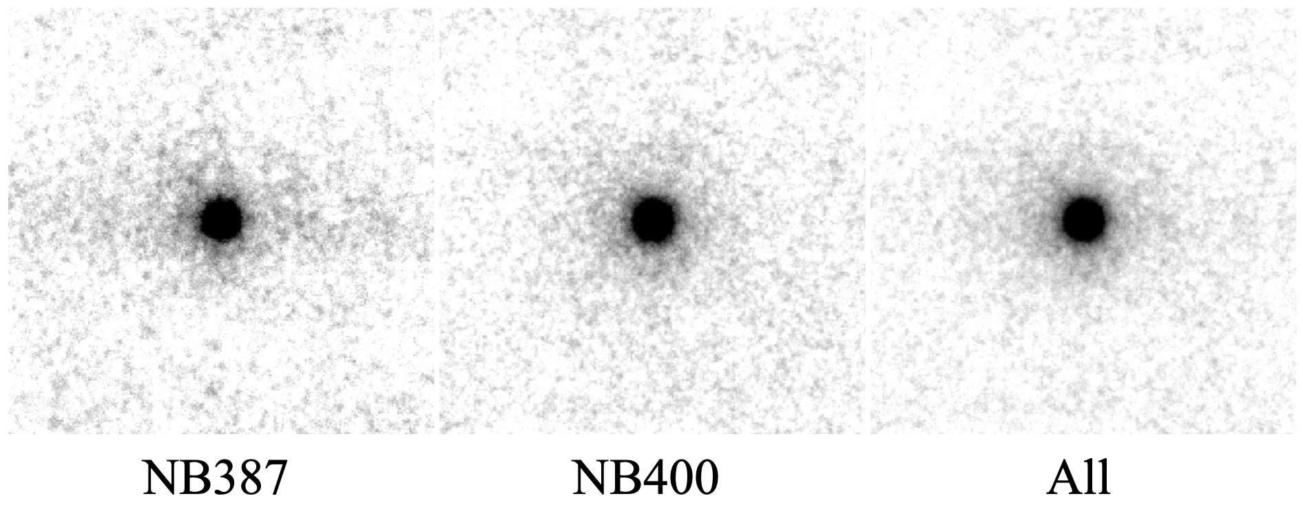
Figure 2: Stacked Ly$\alpha$ images of NB387, NB400, all LAEs. The size of each image is $50^{\prime\prime}.4\times 50^{\prime\prime}.4$ ($\sim 415\times 415$ kpc²). The lower and upper surface brightness limits for plotting the images are 0 and $2\times 10^{-18}$ erg s^-1 cm^-2 arcsec^-2, respectively.

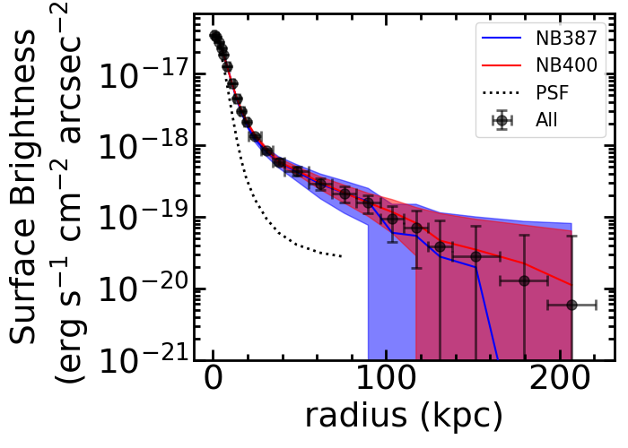
Figure 3: Ly$\alpha$ surface brightness profiles of NB387 (blue), NB400 (red), all (black) LAEs. The horizontal error bars indicate the ranges of radius bins, while the vertical error bars are the uncertainties of surface brightness obtained by our simulation. The point-spread-function (PSF; dotted line) is obtained by stacking 533 point sources with NB magnitudes of $18-22$ mag. We scale the PSF to the all profile at the radius of $\sim 0$ kpc for comparison, while the NB387, NB400, and all profiles are not scaled.

We compare our stacking result with previous LAH studies at $z=2-3$ as shown in Figure 4. Using a method similar to this study, Momose et al. (2014; hereafter M14) stack 3556 LAEs at $z=2.2$ with Subaru/Suprime-Cam and identify LAH extended to $\sim 80$ kpc. Our result is consistent with M14 after scaling, although the uncertainty of M14 is relatively large at radii larger than 30 kpc. We also compare our results with Lujan Niemeyer et al. (2022; hereafter N22). N22 stack 968 spectroscopically confirmed LAEs at $z=1.9-3.5$ with the HETDEX data, and identify Ly$\alpha$ emission extended to 320 kpc. Our result is consistent with N22 at radii smaller than $\sim 25$ kpc, but is more extended at radii of $\sim 25-100$ kpc. Further at radii of $\sim 100-200$ kpc, there are no clear differences between N22 and our result beyond the error bars. The N22 halos seem to be more extended than this study at radii larger than 200 kpc, although the last bin size of N22 is large ($160-320$ kpc). By this comparison, the most notable difference is at radii of $\sim 25-100$ kpc.

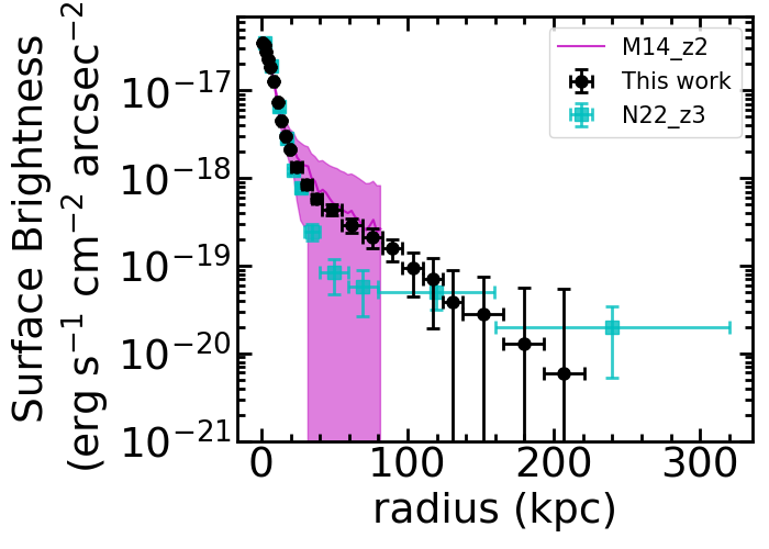
Figure 4: Ly$\alpha$ surface brightness profiles of Momose et al. (2014; magenta) and Lujan Niemeyer et al. (2022; cyan) compared with this study (black). We scale the profiles of M14 and N22 to this study at the radius of $\approx 0$ kpc for comparison.

The reason causing this difference is not clear. The difference is not likely caused by the contamination in our LAEs, because the contamination rate of our LAE candidates is low (8%; see Section 4) and we use a median stacking method, the contribution from the contamination is expected to be small ($\lesssim 8\%$). Moreover, the contamination is typically foreground point sources that make the surface brightness profile more compact, which cannot explain our more extended profile compared to N22. There are two possibilities that cause the different results. The first possibility is the redshift difference. N22 stack LAEs with a larger redshift range ($z=1.9-3.5$) than our LAEs ($z=2.2-2.3$) to increase their sample size, and a possible evolution of LAHs from $z=3$ to 2 may cause the difference. Indeed, it is shown that LAHs at $z=2$ are 0.4 dex fainter than those at $z=3$ at radii smaller than $\sim 100$ kpc (Cai et al. 2019). However, this evolution from $z=3$ to 2 does not greatly change the profile shape (slope), and the redshift evolution alone may not explain the difference between N22 and our results. The second possibility is the field difference. Our fields are either selected based on a high HI density along background QSO sightlines, or selected to contain multiple QSOs (see Cai et al. 2016, Liang et al. 2021, and Cai et al. in prep. for details). As a result, our special field selection may cause the different LAHs. Note that there are several other stacking studies at $z=2-3$ such as Wisotzki et al. (2018) and Kikuchihara et al. (2022). Because results from these studies are similar to M14 and N22, and their surface brightness limits are not as deep as N22, we only compare our results to M14 and N22.

5.2 Connection between Central Galaxies and LAHs

To investigate how central galaxies affect the surrounding LAHs, we divide our LAEs into subsamples based on Ly$\alpha$ luminosity ($L_{\rm Ly\alpha}$), rest-frame Ly$\alpha$ equivalent width (EW₀), and UV magnitude (M_uv). If properties ($L_{\rm Ly\alpha}$, EW₀, and M_uv) of a LAE is smaller than the median values, we assign this LAE to the low sample. On the opposite, we assign a LAE to the high sample if its properties are larger than the median values. Each subsample thus contains one half of the all sample. The median properties of the subsamples are summarized in Table 2.

Table 2: Properties of subsamples

Sample	$\log(L_{\rm Ly\alpha})$	EW0	Muv
name	erg s-1	Å	mag
L_low	42.24	59.9	-18.63
L_high	42.67	64.5	-19.73
EW_low	42.40	34.1	-19.77
EW_high	42.45	98.1	-18.51
Muv_low	42.69	38.1	-20.15
Muv_high	42.30	90.5	-18.53
all	42.41	52.2	-19.40

Note. — Column 1: sample name; Column 2: median Ly$\alpha$ luminosity; Column 3: median rest-frame Ly$\alpha$ equivalent width; Column 4: median UV magnitude.

We stack the subsamples separately using the same method in Section 5.1. Figure 5 shows the stacking results of our subsamples. The subsamples show clear differences at the radii of $\sim 10-40$ kpc. We find that higher $L_{\rm Ly\alpha}$, lower EW₀, and brighter M_uv cause more extended LAHs. Because the three properties are correlated and more massive LAEs generally have higher $L_{\rm Ly\alpha}$, lower EW₀, and brighter M_uv (see Muv_low and Muv_high subsamples in Table 2), our results suggest that more massive LAEs generally have more extended halos. Similar results have also been shown in Zhang et al. (2020).

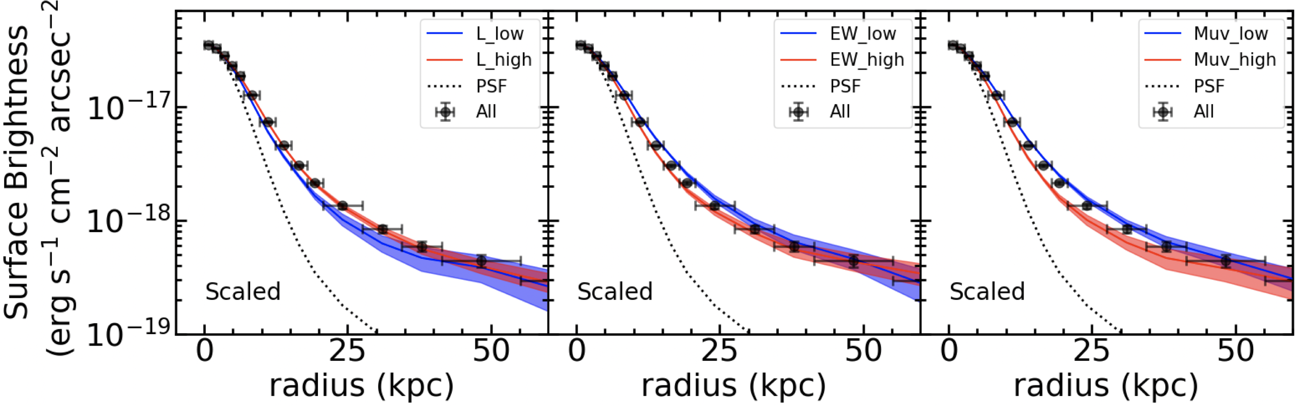
Figure 5: Ly$\alpha$ surface brightness profiles of our subsamples (blue for low and red for high) divided based on $L_{\rm Ly\alpha}$ (left), EW₀ (middle), and M_uv (right). All of the profiles are scaled at the radius of $\sim 0$ kpc for comparison.

Because LAEs with higher $L_{\rm Ly\alpha}$ generally have more extended halos, we investigate whether the halo difference between N22 and our result is caused by luminosity differences. The median Ly$\alpha$ luminosities of L_low, L_high, and N22 are 42.2, 42.7, and 42.8 erg s^-1, respectively. Because a higher $L_{\rm Ly\alpha}$ corresponds to a more extended profile, the profile of N22 is expected to be more extended than those of L_low and L_high. However, we find that the profile of N22 is clearly more compact at the radii of $\sim 25-100$ kpc, as shown in Figure 6. This comparison suggests that our more extended Ly$\alpha$ halo compared to N22 cannot be explained by the luminosity difference, but instead by other reasons such as the two possibilities we discussed in Section 5.1.

Previous studies have also investigated the connection between central galaxies and LAHs as we briefly introduced in Section 1. Momose et al. (2016) also find that galaxies with lower EW₀ and brighter M_uv have more extended halos. However, galaxies with higher $L_{\rm Ly\alpha}$ show less extended halos in Momose et al. (2016), which is opposite to this study. Xue et al. (2017) find that galaxies with higher $L_{\rm Ly\alpha}$ and brighter M_uv have more extended halos, but the halo correlation with EW₀ is not clear. It should be noted that the halos in Momose et al. (2016) and Xue et al. (2017) are only identified at radii smaller than $80$ kpc and have larger uncertainties than this study. Similarly, N22 also show that halo becomes more extended for a higher $L_{\rm Ly\alpha}$, but the relations with EW₀ and M_uv are not investigated. In summary, the relation between central galaxy properties ($L_{\rm Ly\alpha}$, EW₀, and M_uv) and LAHs in this study is consistent with most previous studies.

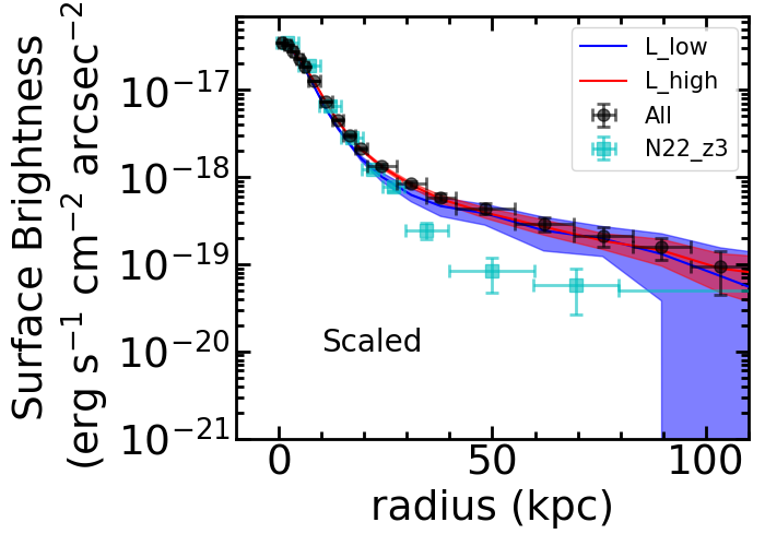
Figure 6: Ly$\alpha$ surface brightness profiles of our subsamples (blue for low and red for high) and all sample (black) compared with N22 (cyan). All of the profiles are scaled at the radius of $\sim 0$ kpc for comparison.

6 Summary

In this study, we identify the Ly$\alpha$ halo extended to $\sim 200$ kpc by stacking $\sim 3300$ Ly$\alpha$ emitters at $z=2.2-2.3$. Our results are summarized below.

1. We carry out imaging observations and data reduction with Subaru/HSC. The total survey area is $\sim 12$ deg² and imaging depths are $25.5-27.0$ mag. Using the imaging data, we select 1240 and 2101 LAE candidates at $z=2.2$ and 2.3, respectively.

2. We carry out spectroscopic observations of our LAE candidates and data reduction with Magellan/IMACS to estimate the contamination rate of our LAE candidates. We find that the contamination rate of our sample is low (8%).

3. We stack our LAE candidates with a median stacking method to identify the Ly$\alpha$ halo at $z=2$. We find that the Ly$\alpha$ halo is extended to $\sim 200$ kpc at a surface brightness level of $10^{-20}$ erg s^-1 cm^-2 arcsec^-2.

4. Comparing to previous studies, our Ly$\alpha$ halo is consistent with M14 after scaling, but is clearly more extended than N22 at radii of $\sim 25-100$ kpc. The halo difference is not likely caused by the contamination in our sample, but by redshift and/or field differences instead.

5. We divide our LAEs into subsamples based on Ly$\alpha$ luminosity ($L_{\rm Ly\alpha}$), rest-frame Ly$\alpha$ equivalent width (EW₀), and UV magnitude (M_uv). We stack the subsamples and find clear differences between the subsamples at radii of $\sim 10-40$ kpc. Our result shows that higher $L_{\rm Ly\alpha}$, lower EW₀, and brighter M_uv cause more extended halos, which suggests that more massive LAEs generally have more extended Ly$\alpha$ halos.

The Hyper Suprime-Cam (HSC) collaboration includes the astronomical communities of Japan and Taiwan, and Princeton University. The HSC instrumentation and software were developed by the National Astronomical Observatory of Japan (NAOJ), the Kavli Institute for the Physics and Mathematics of the Universe (Kavli IPMU), the University of Tokyo, the High Energy Accelerator Research Organization (KEK), the Academia Sinica Institute for Astronomy and Astrophysics in Taiwan (ASIAA), and Princeton University. Funding was contributed by the FIRST program from Japanese Cabinet Office, the Ministry of Education, Culture, Sports, Science and Technology (MEXT), the Japan Society for the Promotion of Science (JSPS), Japan Science and Technology Agency (JST), the Toray Science Foundation, NAOJ, Kavli IPMU, KEK, ASIAA, and Princeton University.

This paper makes use of software developed for the Large Synoptic Survey Telescope. We thank the LSST Project for making their code available as free software at http://dm.lsst.org

The Pan-STARRS1 Surveys (PS1) have been made possible through contributions of the Institute for Astronomy, the University of Hawaii, the Pan-STARRS Project Office, the Max-Planck Society and its participating institutes, the Max Planck Institute for Astronomy, Heidelberg and the Max Planck Institute for Extraterrestrial Physics, Garching, The Johns Hopkins University, Durham University, the University of Edinburgh, Queen’s University Belfast, the Harvard-Smithsonian Center for Astrophysics, the Las Cumbres Observatory Global Telescope Network Incorporated, the National Central University of Taiwan, the Space Telescope Science Institute, the National Aeronautics and Space Administration under Grant No. NNX08AR22G issued through the Planetary Science Division of the NASA Science Mission Directorate, the National Science Foundation under Grant No. AST-1238877, the University of Maryland, and Eotvos Lorand University (ELTE) and the Los Alamos National Laboratory.

Based in part on data collected at the Subaru Telescope and retrieved from the HSC data archive system, which is operated by Subaru Telescope and Astronomy Data Center at National Astronomical Observatory of Japan.

The authors wish to recognize and acknowledge the very significant cultural role and reverence that the summit of Maunakea has always had within the indigenous Hawaiian community. We are most fortunate to have the opportunity to conduct observations from this mountain.

This paper includes data gathered with the 6.5 meter Magellan Telescopes located at Las Campanas Observatory, Chile.

Appendix A Surface Brightness Distribution of Sky

References

- Aihara et al. (2018) Aihara, H., Arimoto, N., Armstrong, R., et al. 2018, PASJ, 70, S4
- Arrigoni Battaia et al. (2019) Arrigoni Battaia, F., Hennawi, J. F., Prochaska, J. X., et al. 2019, MNRAS, 482, 3162. doi:10.1093/mnras/sty2827
- Bertin & Arnouts (1996) Bertin, E. & Arnouts, S. 1996, A&AS, 117, 393. doi:10.1051/aas:1996164
- Bosch et al. (2018) Bosch, J., Armstrong, R., Bickerton, S., et al. 2018, PASJ, 70, S5
- Cai et al. (2016) Cai, Z., Fan, X., Peirani, S., et al. 2016, ApJ, 833, 135. doi:10.3847/1538-4357/833/2/135
- Cai et al. (2019) Cai, Z., Cantalupo, S., Prochaska, J. X., et al. 2019, ApJS, 245, 23. doi:10.3847/1538-4365/ab4796
- Feldmeier et al. (2013) Feldmeier, J. J., Hagen, A., Ciardullo, R., et al. 2013, ApJ, 776, 75
- Furusawa et al. (2018) Furusawa, H., Koike, M., Takata, T., et al. 2018, PASJ, 70, S3
- Hayashino et al. (2004) Hayashino, T., Matsuda, Y., Tamura, H., et al. 2004, AJ, 128, 2073
- Kakuma et al. (2021) Kakuma, R., Ouchi, M., Harikane, Y., et al. 2021, ApJ, 916, 22. doi:10.3847/1538-4357/ac0725
- Kawanomoto et al. (2018) Kawanomoto, S., Uraguchi, F., Komiyama, Y., et al. 2018, PASJ, 70, 66
- Kikuchihara et al. (2022) Kikuchihara, S., Harikane, Y., Ouchi, M., et al. 2022, ApJ, 931, 97. doi:10.3847/1538-4357/ac69de
- Komiyama et al. (2018) Komiyama, Y., Obuchi, Y., Nakaya, H., et al. 2018, PASJ, 70, S2
- Konno et al. (2016) Konno, A., Ouchi, M., Nakajima, K., et al. 2016, ApJ, 823, 20. doi:10.3847/0004-637X/823/1/20
- Leclercq et al. (2017) Leclercq, F., Bacon, R., Wisotzki, L., et al. 2017, A&A, 608, A8
- Liang et al. (2021) Liang, Y., Kashikawa, N., Cai, Z., et al. 2021, ApJ, 907, 3. doi:10.3847/1538-4357/abcd93
- Lujan Niemeyer et al. (2022) Lujan Niemeyer, M., Komatsu, E., Byrohl, C., et al. 2022, ApJ, 929, 90. doi:10.3847/1538-4357/ac5cb8
- Magnier et al. (2013) Magnier, E. A., Schlafly, E., Finkbeiner, D., et al. 2013, The Astrophysical Journal Supplement Series, 205, 20
- Matsuda et al. (2012) Matsuda, Y., Yamada, T., Hayashino, T., et al. 2012, MNRAS, 425, 878
- Miyazaki et al. (2018) Miyazaki, S., Komiyama, Y., Kawanomoto, S., et al. 2018, PASJ, 70, S1
- Momose et al. (2014) Momose, R., Ouchi, M., Nakajima, K., et al. 2014, MNRAS, 442, 110
- Momose et al. (2016) Momose, R., Ouchi, M., Nakajima, K., et al. 2016, MNRAS, 457, 2318
- Oke & Gunn (1983) Oke, J. B., & Gunn, J. E. 1983, ApJ, 266, 713
- Rauch et al. (2008) Rauch, M., Haehnelt, M., Bunker, A., et al. 2008, ApJ, 681, 856
- Schlafly et al. (2012) Schlafly, E. F., Finkbeiner, D. P., Jurić, M., et al. 2012, ApJ, 756, 158
- Steidel et al. (2011) Steidel, C. C., Bogosavljević, M., Shapley, A. E., et al. 2011, ApJ, 736, 160
- Tonry et al. (2012) Tonry, J. L., Stubbs, C. W., Lykke, K. R., et al. 2012, ApJ, 750, 99
- Wisotzki et al. (2016) Wisotzki, L., Bacon, R., Blaizot, J., et al. 2016, A&A, 587, A98
- Wisotzki et al. (2018) Wisotzki, L., Bacon, R., Brinchmann, J., et al. 2018, Nature, 562, 229
- Xue et al. (2017) Xue, R., Lee, K.-S., Dey, A., et al. 2017, ApJ, 837, 172. doi:10.3847/1538-4357/837/2/172
- Zhang et al. (2020) Zhang, H., Ouchi, M., Itoh, R., et al. 2020, ApJ, 891, 177. doi:10.3847/1538-4357/ab7917