MAMMOTH-Subaru IV. Large Scale Structure and Clustering Analysis of Ly Emitters and Ly Blobs at
Abstract
We report the large scale structure and clustering analysis of Ly emitters (LAEs) and Ly blobs (LABs) at . Using 3,341 LAEs, 117 LABs, and 58 bright (Ly luminosity erg s-1) LABs at selected with Subaru/Hyper Suprime-Cam (HSC), we calculate the LAE overdensity to investigate the large scale structure at . We show that 74% LABs and 78% bright LABs locate in overdense regions, which is consistent with the trend found by previous studies that LABs generally locate in overdense regions. We find that one of our 8 fields dubbed J1349 contains of our LABs and of our bright LABs. A unique and overdense ( comoving Mpc2) region in J1349 has 12 LABs (8 bright LABs). By comparing to SSA22 that is one of the most overdense LAB regions found by previous studies, we show that the J1349 overdense region contains times more bright LABs than the SSA22 overdense region. We calculate the angular correlation functions (ACFs) of LAEs and LABs in the unique J1349 field and fit the ACFs with a power-law function to measure the slopes. The slopes of LAEs and LABs are similar, while the bright LABs show a times larger slope suggesting that bright LABs are more clustered than faint LABs and LAEs. We show that the amplitudes of ACFs of LABs are higher than LAEs, which suggests that LABs have a times larger galaxy bias and field-to-field variance than LAEs. The strong field-to-field variance is consistent with the large differences of LAB numbers in our 8 fields.
1 Introduction
In the last two decades, luminous and spatially extended Ly emitters (LAEs) have been identified at by wide-field imaging surveys. These luminous and extended LAEs are often referred to as Ly blobs (LABs; e.g. Keel et al. 1999; Steidel et al. 2000; Matsuda et al. 2004; Ouchi et al. 2009; Yang et al. 2009; Sobral et al. 2015; Cai et al. 2017; Shibuya et al. 2018; Kikuta et al. 2019; Zhang et al. 2020; Li et al. in prep.). The Ly luminosities of LABs are commonly brighter than erg s-1, and the sizes are much larger than point sources. The luminous and extended nature of LABs allows the detection of Ly emission in the circumgalactic medium (CGM) scale at high- even with a limited imaging depth. Because Ly emission traces the hydrogen gas in the CGM, it is widely believed that LABs are important objects to study formation and evolution of galaxies in the early Universe.
Previous studies have shown that LABs are commonly located in overdense regions, suggesting that the formation of LABs is affected by the environment such as the large scale structure (e.g. Francis et al. 1996; Steidel et al. 2000; Yang et al. 2009; Matsuda et al. 2011; Kikuta et al. 2019; Zhang et al. 2020). The field-to-field variation of LABs is found to be strong (Yang et al. 2010). One of the densest LAB fields found by previous studies is the SSA22 field at . In a ( cMpc2) region of the SSA22 field, 35 LABs have been identified (Matsuda et al. 2004). Because such a dense LAB field is very rare, the discovery strongly depends on wide-field surveys and the identification of new dense LAB fields provides important insight on the extreme galaxy formation environment.
Clustering analysis using methods such as the angular correlation function (ACF) is important for understanding the spatial distribution of galaxies. Although the ACF of LAEs has been investigated at high- (e.g. Ouchi et al. 2010; Harikane et al. 2016), limited information about the ACF of LABs can be found from the literature yet. By comparing the ACFs of LAEs and LABs, one can understand if the underlying dark matter halos affect the formation of LAEs and LABs similarly.
In this paper, we investigate the large scale structure and carry out clustering analysis of LAEs and LABs at . This paper is organized as follows. In Section 2, we introduce our observations and data reduction. Using the reduced data, we show our selection of LAEs and LABs in Section 3. The results and discussion are presented in Section 4. Finally, we summarize this paper in Section 5. The AB magnitudes (Oke & Gunn, 1983) and physical distances are used throughout this paper unless indicated otherwise. We adopt the CDM cosmology with , , and .
2 Observations and Data Reduction
The imaging data we use in this study are obtained with Subaru/Hyper Suprime-Cam (HSC; Miyazaki et al. 2018; Komiyama et al. 2018; Kawanomoto et al. 2018; Furusawa et al. 2018). We carry out observations using narrowband (NB387 and NB400) and broadband () filters between January 2018 and March 2020. The NB387, NB400, and filters are centered at 3863, 4003, and 4754 Å, respectively. The filter widths (FWHM) of NB387, NB400, and are 55, 92, and 1395 Å, respectively. The observations are carried out in 8 fields with a total survey area of deg2. Details of the field selection are presented in Cai et al. (2016), Liang et al. (2021), Cai et al. (in prep.), and Liang et al. (in prep.). The seeing sizes are between and . We summarize the information of the 8 fields in Table 1.
We reduce the imaging data with the HSC pipeline dubbed hscPipe (Bosch et al. 2018; Aihara et al. 2018). Details of the data reduction in NB387 and NB400 fields are presented in Liang et al. (2021) and Zhang et al. (in prep.), respectively. After data reduction, we measure the detection limits in a diameter aperture, except for J0210 field in a diameter aperture because the seeing in J0210 is the worst. The detection limits are , , and mag for NB387, NB400, and , respectively. The source detection and photometry are carried out with SExtractor (Bertin & Arnouts, 1996) and described in Liang et al. (2021) and Zhang et al. (in prep.). We do not use regions such as those near bright stars and field edges because of the low signal-to-noise ratios (SNRs).
| Field | R.A. (J2000) | Decl. (J2000) | Filters | |||||
|---|---|---|---|---|---|---|---|---|
| name | hh:mm:ss | dd:mm:ss | name | mag | mag | count | count | count |
| J0210 | 02:09:58.90 | +00:53:43.0 | NB387 & | 24.25 | 26.34 | 227 | 10 | 5 |
| J0222 | 02:22:24.66 | -02:23:41.2 | NB387 & | 24.99 | 27.01 | 422 | 10 | 4 |
| J0924 | 09:24:00.70 | +15:04:16.7 | NB387 & | 24.74 | 26.63 | 311 | 5 | 2 |
| J1419 | 14:19:33.80 | +05:00:17.2 | NB387 & | 24.81 | 26.80 | 280 | 12 | 3 |
| J0240 | 02:40:05.11 | -05:21:06.7 | NB400 & | 25.61 | 26.80 | 517 | 24 | 16 |
| J0755 | 07:55:35.89 | +31:09:56.9 | NB400 & | 25.83 | 26.50 | 545 | 9 | 4 |
| J1133 | 11:33:02.40 | +10:05:06.0 | NB400 & | 25.49 | 26.30 | 403 | 8 | 2 |
| J1349 | 13:49:40.80 | +24:28:48.0 | NB400 & | 25.67 | 26.15 | 636 | 39 | 22 |
Note. — Column 1: field name; Column 2: right ascension; Column 3: declination; Column 4: filter name; Column 5: 5 limiting magnitude of narrowband; Column 6: 5 limiting magnitude of broadband; Column 7: number of LAE candidates selected in this study: Column 8: number of LAB candidates selected in this study; Column 9: number of bright LAB candidates selected in this study.
3 Sample Selection
Similar to previous studies (e.g. Konno et al. 2016; Liang et al. 2021), we select LAEs with a narrowband minus broadband (NB-BB) color excess that corresponds to a rest-frame Ly equivalent width of Å. Details of our LAE selection are presented in Liang et al. (2021) and Zhang et al. (in prep.). In brief, NB387 LAEs are selected with the following criteria:
| (1) |
where the subscripts “ap” and “tot” are the aperture and total magnitudes, respectively. The “AUTO” magnitude in SExtrator is used as the total magnitude. For sources whose magnitudes are fainter than the limit, we use the limit instead. We calculate the color uncertainty by , where and are the uncertainties in and NB387, respectively. We then visually inspect sources passing the criteria and remove spurious sources such as cosmic rays and satellite trails. Our final NB387 LAE catalog contains 1,240 candidates.
Similarly, NB400 LAEs are selected with the following criteria:
| (2) |
where we use the same symbols as Equation 1. We carry out visual inspection after applying the selection criteria to remove spurious sources such as cosmic rays and satellite trails. Our final NB400 LAE catalog contains 2101 candidates after visual inspection. The number of LAE candidates in each field is presented in Table 1.
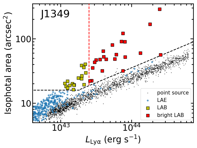
After obtaining the LAE catalogs, we select LABs based on the Ly luminosity and isophotal area as shown in Li et al. (in prep.; Figure 1). We define the isophotal area using the area above the 2 surface brightness limit. We select LABs with an isophotal area larger than 3 confidence levels of the point sources. The isophotal area should also be larger than a minimum value that depends on the depth of each field (see details in Li et al. in prep.). After applying the criteria, we carry out visual inspection to remove sources whose isophotal areas are affected by adjacent artifacts or bright stars. After visual inspection, we select 37 and 80 LAB candidates at and 2.3, respectively. Among these LAB candidates, we further select LABs with Ly luminosities larger than erg s-1, and these LABs are referred to as bright LABs hereafter. The selection of bright LABs is an empirical criterion adopted by previous studies (e.g. Shibuya et al. 2018; Zhang et al. 2020), and we use this criterion for a comparison in Section 4. The numbers of bright LABs are 14 and 44 at and 2.3, respectively. The number of LABs in each field is presented in Table 1.
4 Results and Discussion
4.1 LAE Overdensity
To investigate the large scale structure in our 8 fields, we calculate the LAE overdensity. The LAE overdensity is defined by
| (3) |
where and are the number and field-averaged number of LAEs in a circular aperture, respectively. The is calculated in each field separately. The diameter of the aperture is 20 comoving Mpc (cMpc) that is consistent with previous studies at (e.g. Liang et al. 2021). We assume the Poisson statistics for and in our calculation. Figure 2 shows the LAE overdensity map of the 8 fields along with our LABs. We find that 86 out of 117 LABs and 45 out of 58 bright LABs locate in overdense regions. The overdense fractions are 86/117=74% and 45/58=78% for LABs and bright LABs, respectively. This result is consistent with the trend found by previous studies that LABs generally locate in overdense regions (e.g. Bădescu et al. 2017; Kikuta et al. 2019; Zhang et al. 2020).
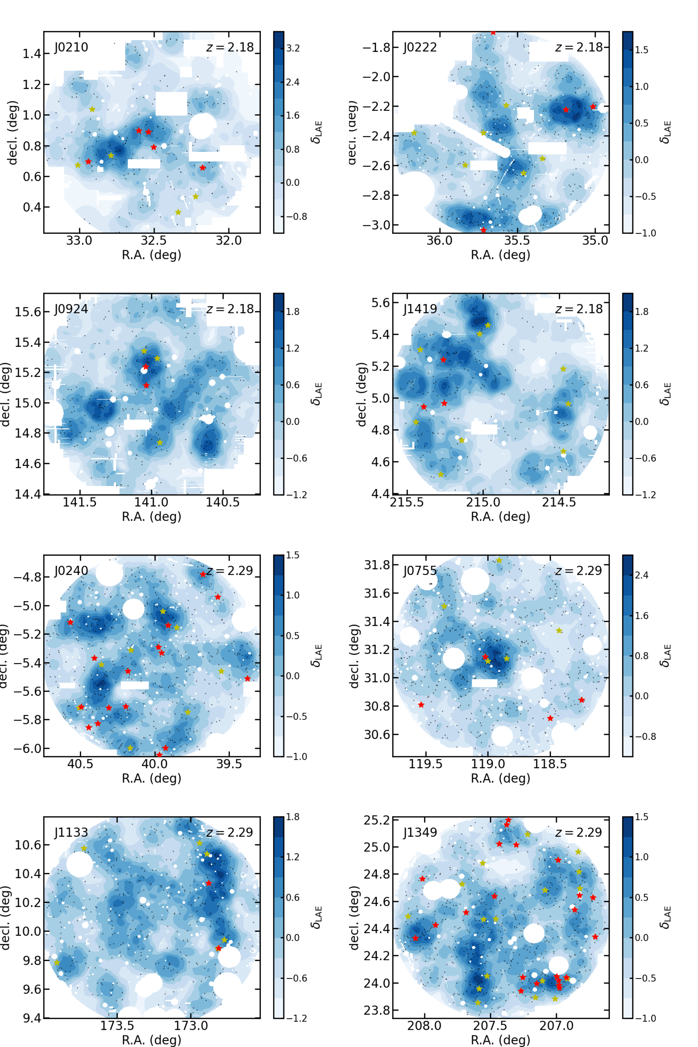
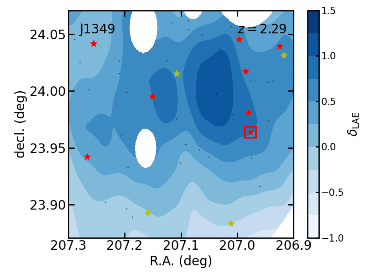
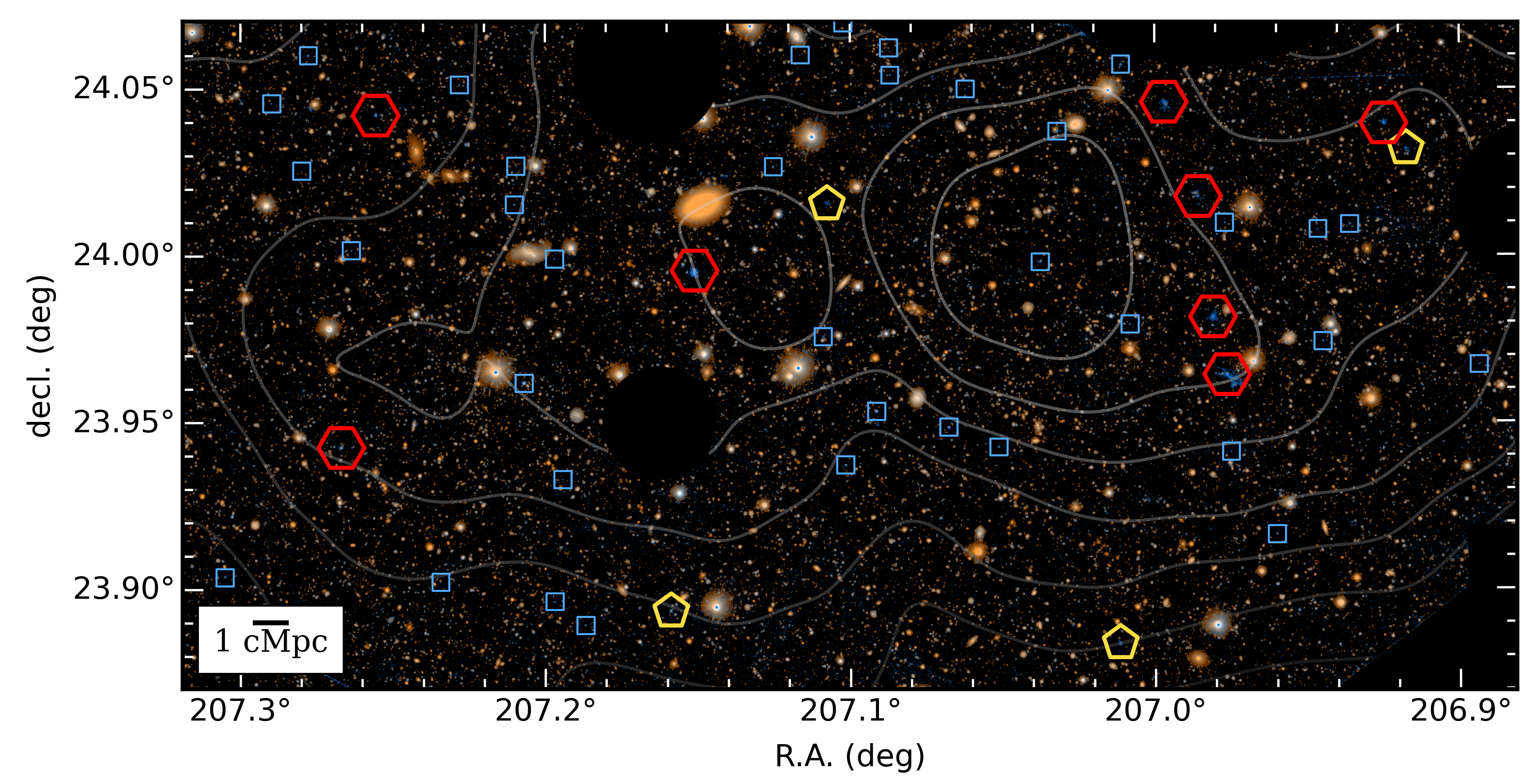
Interestingly, we find that the J1349 field contains of our LABs and of our bright LABs. The J1349 field shows an overdense ( cMpc2) region (Figure 3 and 4) that has 12 LABs (8 bright LABs). This region is referred to the J1349 overdense region hereafter while the J1349 field means the whole field of view. We compare the J1349 overdense region with one of the most overdense LAB regions found by previous studies. Matsuda et al. (2004) identify 35 LABs in a ( cMpc2) region of the SSA22 field at . Four out of these 35 LABs are bright LABs with erg s-1. Because Matsuda et al. (2004) use different isophotal area selection criteria ( arcsec2) from our selection, it is not fair to directly compare the LAB numbers. On the other hand, of sources at different redshifts can be directly compared. Thus, we apply the same cut ( erg s-1) for Matsuda et al. (2004) and our sample, and only compare the number of bright LABs. The survey volumes of the J1349 and SSA22 overdense regions are and cMpc, respectively. The volume densities of bright LABs are then and cMpc-3 for the J1349 and SSA22 overdense regions, respectively. If we use a same survey volume of cMpc, the volume density of bright LABs in the J1349 overdense region becomes cMpc-3. This comparison shows that the J1349 overdense region contains times more bright LABs than the SSA22 overdense region.
4.2 Angular Correlation Function
To further investigate the unique J1349 field, we calculate the angular correlation functions (ACFs) of LAEs and LABs. We calculate the ACF with the following equation:
| (4) |
where , , and are the numbers of galaxy-galaxy, galaxy-random, and random-random pairs divided by the total number of pairs in galaxy-galaxy, galaxy-random, and random-random samples, respectively (Landy & Szalay 1993). The random sample contains 100,000 randomly generated points. We take the masks in 8 fields into consideration when making the random sample. We estimate the uncertainty of by assuming that , , and follow the Poisson distribution (Gehrels 1986).
Figure 5 shows the ACFs of our LAEs and LABs in the J1349 field. We fit the ACFs with a power-law function and measure the amplitude and slope . The best-fit slopes of LAEs, LABs, and bright LABs are , , and , respectively. The slopes of LAEs and LABs are similar, while the bright LABs show a times larger slope. This result suggests that bright LABs are more clustered than faint LABs and LAEs. Similarly, Herrero Alonso et al. (2023) find that luminous LAEs are more clustered and reside in more massive dark matter halos than faint LAEs.
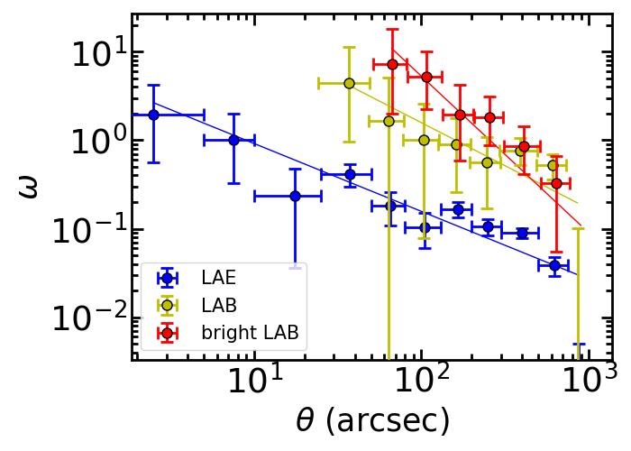
It should be noted that the amplitudes of ACFs of LABs are times higher than LAEs. This is not likely caused by the contamination such as foreground sources in our LAEs, because the contamination rate is low (8%; Zhang et al. in prep.). The high amplitudes suggest that LABs have a times higher galaxy bias than LAEs (cf. Ouchi et al. 2010; Moster et al. 2010). Because the cosmic variance is given by , where is the density fluctuation of dark matter and is expected to be nearly constant for the same redshift and survey volume, the large bias causes a large of LABs. The large is consistent with the strong field-to-field variance of LAB numbers found in this study and in the literature (e.g., Yang et al. 2010).
5 Summary
In this study, we investigate the large scale structure and carry out clustering analysis of LAEs and LABs at . Our results are summarized below.
-
1.
Using 3341 LAEs, 117 LABs, and 58 bright (Ly luminosity erg s-1) LABs at , we calculate the LAE overdensity to investigate the large scale structure at . We show that 74% LABs and 78% bright LABs locate in overdense regions, which is consistent with the trend found by previous studies that LABs generally locate in overdense regions.
-
2.
We find that the J1349 field contains of our LABs and of our bright LABs. A unique and overdense ( comoving Mpc2) region in J1349 has 12 LABs (8 bright LABs). By comparing to SSA22 that is one of the most overdense LAB regions found by previous studies, we show that the J1349 overdense region contains times more bright LABs than the SSA22 overdense region.
-
3.
We calculate the angular correlation functions of LAEs and LABs in the unique J1349 field and fit the ACFs with a power-law function to measure the slopes. The best-fit slopes of LAEs, LABs, and bright LABs are , , and , respectively. The slopes of LAEs and LABs are similar, while the bright LABs show a times larger slope. This suggests that bright LABs are more clustered than faint LABs and LAEs.
-
4.
We show that the amplitudes of ACFs of LABs are higher than LAEs, which suggests that LABs have a times larger galaxy bias and field-to-field variance than LAEs. The strong field-to-field variance is consistent with the large differences of LAB numbers in our 8 fields.
The Hyper Suprime-Cam (HSC) collaboration includes the astronomical communities of Japan and Taiwan, and Princeton University. The HSC instrumentation and software were developed by the National Astronomical Observatory of Japan (NAOJ), the Kavli Institute for the Physics and Mathematics of the Universe (Kavli IPMU), the University of Tokyo, the High Energy Accelerator Research Organization (KEK), the Academia Sinica Institute for Astronomy and Astrophysics in Taiwan (ASIAA), and Princeton University. Funding was contributed by the FIRST program from Japanese Cabinet Office, the Ministry of Education, Culture, Sports, Science and Technology (MEXT), the Japan Society for the Promotion of Science (JSPS), Japan Science and Technology Agency (JST), the Toray Science Foundation, NAOJ, Kavli IPMU, KEK, ASIAA, and Princeton University.
This paper makes use of software developed for the Large Synoptic Survey Telescope. We thank the LSST Project for making their code available as free software at http://dm.lsst.org
The Pan-STARRS1 Surveys (PS1) have been made possible through contributions of the Institute for Astronomy, the University of Hawaii, the Pan-STARRS Project Office, the Max-Planck Society and its participating institutes, the Max Planck Institute for Astronomy, Heidelberg and the Max Planck Institute for Extraterrestrial Physics, Garching, The Johns Hopkins University, Durham University, the University of Edinburgh, Queen’s University Belfast, the Harvard-Smithsonian Center for Astrophysics, the Las Cumbres Observatory Global Telescope Network Incorporated, the National Central University of Taiwan, the Space Telescope Science Institute, the National Aeronautics and Space Administration under Grant No. NNX08AR22G issued through the Planetary Science Division of the NASA Science Mission Directorate, the National Science Foundation under Grant No. AST-1238877, the University of Maryland, and Eotvos Lorand University (ELTE) and the Los Alamos National Laboratory.
Based in part on data collected at the Subaru Telescope and retrieved from the HSC data archive system, which is operated by Subaru Telescope and Astronomy Data Center at National Astronomical Observatory of Japan.
The authors wish to recognize and acknowledge the very significant cultural role and reverence that the summit of Maunakea has always had within the indigenous Hawaiian community. We are most fortunate to have the opportunity to conduct observations from this mountain.
References
- Aihara et al. (2018) Aihara, H., Arimoto, N., Armstrong, R., et al. 2018, PASJ, 70, S4
- Bădescu et al. (2017) Bădescu, T., Yang, Y., Bertoldi, F., et al. 2017, ApJ, 845, 172. doi:10.3847/1538-4357/aa8220
- Bertin & Arnouts (1996) Bertin, E. & Arnouts, S. 1996, A&AS, 117, 393. doi:10.1051/aas:1996164
- Bosch et al. (2018) Bosch, J., Armstrong, R., Bickerton, S., et al. 2018, PASJ, 70, S5
- Cai et al. (2016) Cai, Z., Fan, X., Peirani, S., et al. 2016, ApJ, 833, 135. doi:10.3847/1538-4357/833/2/135
- Cai et al. (2017) Cai, Z., Fan, X., Bian, F., et al. 2017, ApJ, 839, 131. doi:10.3847/1538-4357/aa6a1a
- Francis et al. (1996) Francis, P. J., Woodgate, B. E., Warren, S. J., et al. 1996, ApJ, 457, 490. doi:10.1086/176747
- Furusawa et al. (2018) Furusawa, H., Koike, M., Takata, T., et al. 2018, PASJ, 70, S3
- Gehrels (1986) Gehrels, N. 1986, ApJ, 303, 336
- Harikane et al. (2016) Harikane, Y., Ouchi, M., Ono, Y., et al. 2016, ApJ, 821, 123. doi:10.3847/0004-637X/821/2/123
- Herrero Alonso et al. (2023) Herrero Alonso, Y., Miyaji, T., Wisotzki, L., et al. 2023, arXiv:2301.04133
- Kawanomoto et al. (2018) Kawanomoto, S., Uraguchi, F., Komiyama, Y., et al. 2018, PASJ, 70, 66
- Keel et al. (1999) Keel, W. C., Cohen, S. H., Windhorst, R. A., & Waddington, I. 1999, AJ, 118, 2547
- Kikuta et al. (2019) Kikuta, S., Matsuda, Y., Cen, R., et al. 2019, PASJ, 71, L2
- Komiyama et al. (2018) Komiyama, Y., Obuchi, Y., Nakaya, H., et al. 2018, PASJ, 70, S2
- Konno et al. (2016) Konno, A., Ouchi, M., Nakajima, K., et al. 2016, ApJ, 823, 20. doi:10.3847/0004-637X/823/1/20
- Landy & Szalay (1993) Landy, S. D. & Szalay, A. S. 1993, ApJ, 412, 64. doi:10.1086/172900
- Liang et al. (2021) Liang, Y., Kashikawa, N., Cai, Z., et al. 2021, ApJ, 907, 3. doi:10.3847/1538-4357/abcd93
- Matsuda et al. (2004) Matsuda, Y., Yamada, T., Hayashino, T., et al. 2004, AJ, 128, 569
- Matsuda et al. (2011) Matsuda, Y., Yamada, T., Hayashino, T., et al. 2011, MNRAS, 410, L13. doi:10.1111/j.1745-3933.2010.00969.x
- Miyazaki et al. (2018) Miyazaki, S., Komiyama, Y., Kawanomoto, S., et al. 2018, PASJ, 70, S1
- Moster et al. (2010) Moster, B. P., Somerville, R. S., Maulbetsch, C., et al. 2010, ApJ, 710, 903. doi:10.1088/0004-637X/710/2/903
- Oke & Gunn (1983) Oke, J. B., & Gunn, J. E. 1983, ApJ, 266, 713
- Ouchi et al. (2009) Ouchi, M., Ono, Y., Egami, E., et al. 2009, ApJ, 696, 1164
- Ouchi et al. (2010) Ouchi, M., Shimasaku, K., Furusawa, H., et al. 2010, ApJ, 723, 869. doi:10.1088/0004-637X/723/1/869
- Shibuya et al. (2018) Shibuya, T., Ouchi, M., Konno, A., et al. 2018, PASJ, 70, S14
- Sobral et al. (2015) Sobral, D., Matthee, J., Darvish, B., et al. 2015, ApJ, 808, 139
- Steidel et al. (2000) Steidel, C. C., Adelberger, K. L., Shapley, A. E., et al. 2000, ApJ, 532, 170
- Yang et al. (2009) Yang, Y., Zabludoff, A., Tremonti, C., et al. 2009, ApJ, 693, 1579. doi:10.1088/0004-637X/693/2/1579
- Yang et al. (2010) Yang, Y., Zabludoff, A., Eisenstein, D., et al. 2010, ApJ, 719, 1654. doi:10.1088/0004-637X/719/2/1654
- Zhang et al. (2020) Zhang, H., Ouchi, M., Itoh, R., et al. 2020, ApJ, 891, 177. doi:10.3847/1538-4357/ab7917