Taking advantage of noise in quantum reservoir computing
Abstract
The biggest challenge that quantum computing and quantum machine learning are currently facing is the presence of noise in quantum devices. As a result, big efforts have been put into correcting or mitigating the induced errors. But, can these two fields benefit from noise? Surprisingly, we demonstrate that under some circumstances, quantum noise can be used to improve the performance of quantum reservoir computing, a prominent and recent quantum machine learning algorithm. Our results show that the amplitude damping noise can be beneficial to machine learning, while the depolarizing and phase damping noises should be prioritized for correction. This critical result sheds new light into the physical mechanisms underlying quantum devices, providing solid practical prescriptions for a successful implementation of quantum information processing in nowadays hardware.
I Introduction
Machine learning (ML) is among the most disruptive technological developments of the early 21st century Kreen and Zeilinger (2022); Qiao et al. (2022). However, despite existing ML solutions capable of coping with systems of moderate size, learning more complex patterns often requires the use of a large number of parameters and long training times; this fact conditions its success to having access to high performance computational resources. For this reason, a tremendous interest has recently arisen for a technological field with potential to dramatically improve many of these algorithms: quantum ML (QML). To unravel the full potential of QML algorithms, fault-tolerant computers with millions of qubits and low error-rates are needed. Although the actual realization of these devices is still decades ahead, the so-called noisy intermediate-scale quantum (NISQ) era has been reached. Thanks to NISQ designs, Google recently claimed Arute et al. (2019) to have achieved quantum supremacy Harrow and Montanaro (2017), not without controversy Cho (2019); Liu et al. (2021), with the quantum computers available today. Moreover, an experimental demonstration of quantum speed-up on a NP-hard problem regarding Gaussian Boson sampling Zhong et al. (2019) was recently provided.
One of the biggest challenges of the current quantum devices is the presence of noise. They perform noisy quantum operations with limited coherence time, which affects the performance of quantum algorithms. To overcome this limitation, great effort has been devoted to designing error-correcting methods Zhao and et al. (2022); Ugwuishiwu et al. (2022), which correct the errors in the quantum hardware as the algorithm goes on, and also error-mitigation techniques Takagi et al. (2022); Guo and Yang (2022), which aim to reduce the noise of the outputs after the algorithm has been executed. Recently, Google Quantum AI proved the scalability of error-correcting techniques AI (2023), which is the first step towards fault-tolerant computation. Even though these methods can sometimes successfully reduce quantum noise, a fundamental question still remains open: Can the presence of noise in quantum devices be beneficial for quantum machine learning algorithms?
The aim of this paper is to address this issue in a highly relevant NISQ algorithm: quantum reservoir computing (QRC) Mujal et al. (2021). This algorithm uses random quantum circuits, carefully chosen from a certain family, in order to extract relevant properties from the input data. The measurements of the quantum circuits are then fed to a ML model, which provides the final prediction. This simple learning structure makes of QRC a suitable QML algorithm for NISQ devices. QRs have been used in a wide range of applications, the most common being classical time-series forecasting Fujii and Nakajima (2017); Nakajima et al. (2019); Kutvonen et al. (2020); Chen et al. (2020); Martínez-Peña et al. (2020, 2021). Regarding quantum tasks, the method presented in Ref. Ghosh et al. (2019a) involves the detection of entanglement and computation of associated quantities, which are challenging to measure accurately in experimental setups. Additionally, in Ref. Ghosh et al. (2021), quantum state tomography using a quantum reservoir has been developed. This method enables reconstruction of the unknown density matrix of the input quantum state with only a single measurement on local observables of the reservoir nodes, without requiring correlation detection. QRs have also been used to compute the preparation of desired quantum states, such as anti-bunched and cat states in Ref. Ghosh et al. (2019b) or maximally entangled states, NOON, W, cluster, and discorded states in Ref. Krisnanda et al. (2021).
The design of the QR has recentlty proven to be crucial to guarantee optimal performance in the ML task Martínez-Peña et al. (2021); Domingo et al. (2022). However, these studies use noiseless quantum simulations, which do not take into account the real limitations of current quantum hardware. Thus, whether real, noisy implementations of QRs provide advantage over classical ML methods is still an open question. In Ref. Liu et al. (2022) the presence of noise has recently been used to improve the convergence of variational quantum algorithms.
In this work, QRs are used to solve a quantum chemistry problem, consisting of predicting the first excited energy of the LiH molecule from its gorund state (see Sect. IV.1), which has become a common benchmark for QML Xia and Kais (2018); Kawai and Nakagawa (2020); Domingo et al. (2022). Quantum chemistry is one of the areas where quantum computing has highest potential of outperforming traditional methods Qiao et al. (2022), since the complexity of the problem increases exponentially with the system’s degrees of freedom. The exponential size of the Hilbert space allows to study high-dimensional systems with few quantum computational resources, when compared to classical methods. Our results show that certain types of noise can actually provide a better performance for QRC than noiseless reservoirs. Our numerical experiments are further supported with a theoretical demonstration. Moreover, we provide a practical criterion to decide how to use quantum noise to improve the performance of the algorithm, and also what noise should be a priority to correct.
II Results
The QML task considered in this work consists on predicting the excited electronic energy from the corresponding ground state with energy for the LiH molecule, using noisy QRs. Three noise models are considered in this study: the depolarizing channel, the amplitude damping channel and the phase damping channel. Full description of the QML task and noise models is provided in section Methods below.
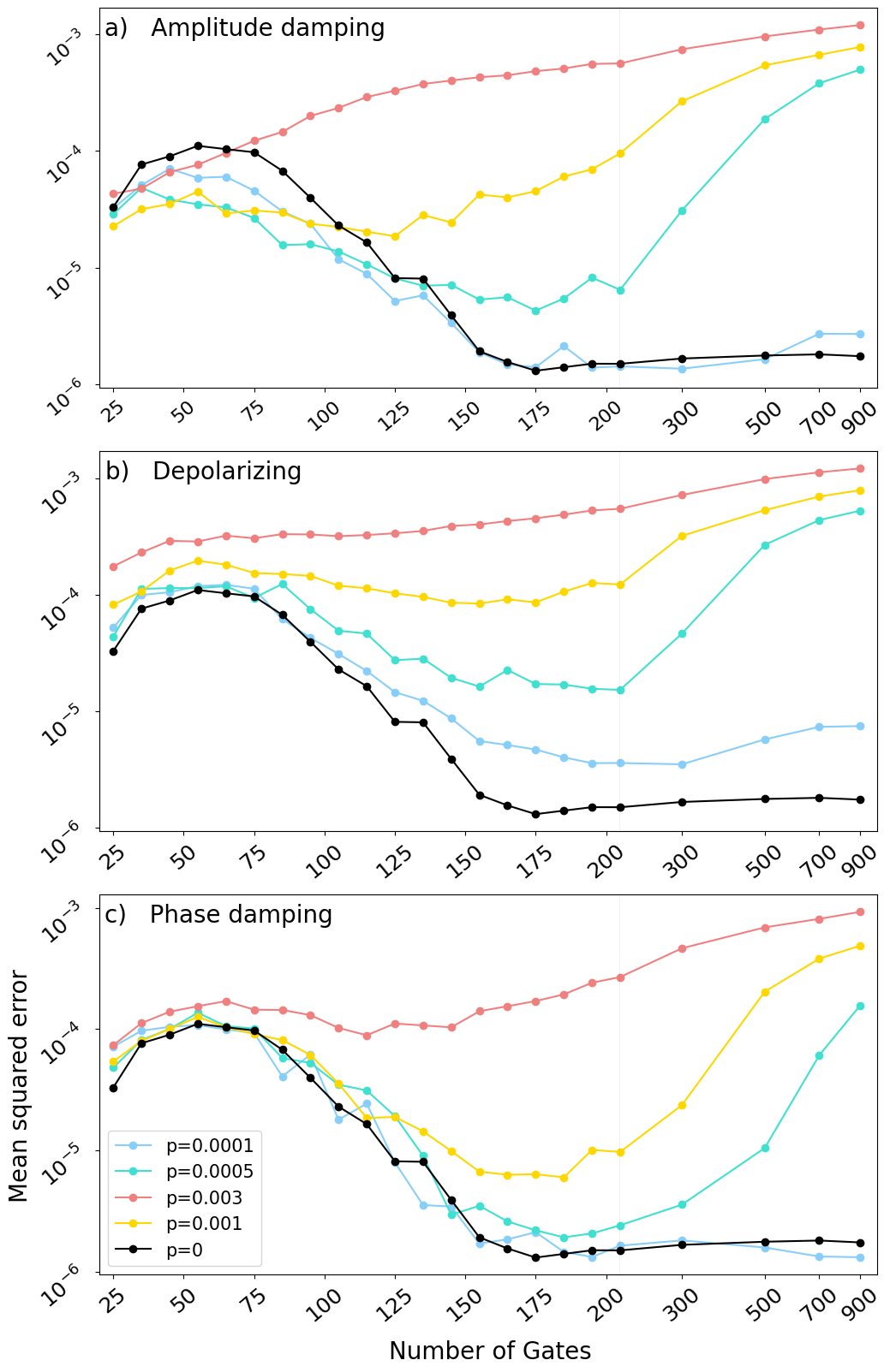
Figure 1 shows the mean squared error (MSE) in predicted with our QRs as a function of the number of gates, for different values of the error probability (colored curves) and noise models (panels), together with the results for the corresponding noiseless reservoir (in black).
As expected, the general tendency of the MSEs is to grow with the noise characterized by . However, a careful comparison of the three plots in Fig. 1 surprisingly demonstrates that the amplitude damping noise renders results which are significantly different from those obtained in the other two cases. Indeed, if the number of gates and error probability are small enough, the QRs with amplitude damping noise provides better results than the noiseless QR. The same conclusion applies for the higher values of , although in those cases the threshold number of gates for better performance decreases. This is a very significant result, since it means that, contrary to the commonly accepted belief, the presence of noise is here beneficial for the performance of the quantum algorithm, and, more importantly, it takes place within the limitations of the NISQ era. As an example, for (green curve) all noisy reservoirs render better performance than the noiseless counterpart when the number of gates is smaller than . Current quantum processors typically have error rates around , which are expected to be significantly reduced soon by employing error-correction techniques AI (2023).
A practical criterion to decide when noise can be used to improve the performance of QRC is provided in Table 1, which shows the averaged fidelity between the output noisy state and the noiseless state for the circuits subjected to an amplitude damping noise with different values of the error probability. The number of gates has been chosen to be as large as possible provided that the noisy reservoirs outperform the noiseless ones. These results imply that when the fidelity is greater than , the noisy reservoirs outperform the noiseless ones at the QML task, and accordingly the noise should not be corrected. Finally, also notice that for the fidelity is always higher than , and thus the performance of the noisy QRs is always higher or equal than their noiseless counterparts. Table 1 also shows that the number of gates needed to outperform the noiseless reservoirs is of the order of 100 quantum gates, which corresponds to an average circuit depth of 10-15 gates. Recently, there have been multiple applications of quantum machine learning algorithms using shallow quantum circuits of similar depth. In particular, multiple shallow quantum neural networks have been combined to solve six benchmark classification problems in Ref. Alam and Ghosh (2022). Also, a hybrid quantum-classical graph neural network, which used quantum circuits of depth10, was developed for particle track reconstruction in particle acceleration experiments Tüysüz et al. (2021). Finally, in Ref. Schatzki et al. (2021), the authors propose the design of quantum datasets for quantum machine learning tasks, where the classification label is encoded in the amount of entanglement of the quantum states. Their results shows that the quantum datasets are successfully implemented with circuit depth smaller than 7. Therefore, quantum circuits with depths of 10-15 gates can provide useful applications in various domains. This is the regime where the amplitude damping noise provides an advantage over noiseless quantum circuits in our setting, which suggests that this type of noise may be beneficial to other quantum machine learning tasks. The extension of this analysis to other applications, such as time series forecasting, will be explored in future works.
| Error prob. | Optimal | Fidelity |
|---|---|---|
| # of gates | (averaged) | |
| 0.0001 | 150 | 0.990 |
| 0.0005 | 135 | 0.965 |
| 0.0010 | 105 | 0.956 |
| 0.0030 | 65 | 0.962 |
A second conclusion from the comparison among plots in Fig. 1 is that the behavior for depolarizing and the phase damping channels is significantly different than for the amplitude damping one. In the former cases, the performance of the noisy reservoirs is always worse than that of the noiseless one, even for small error probabilities.
A third result that can be extracted from our calculations is that the tendency of the algorithm performance when the reservoirs have a large number of gates is the same for the three noise models considered (except for the smallest value of ). While the performance of the noiseless reservoirs stabilizes to a constant value as the number of gates increases, the noisy reservoirs decrease their performance, seemingly going to the same growing behavior. This is due to the fact that the quantum channels are applied after each gate, and thus circuits with a large number of gates have larger noise rates, which highly decreases the fidelity of the output state. For this reason, even though increasing the number of gates has no effect in the noiseless simulations, it highly affects the performance of the noisy circuits, and thus the number of gates should be optimized in this case.
Having analyzed the MSE results, we next provide a theoretical explanation for the different behavior of the three noisy reservoirs. In the first place, the depolarizing and phase damping channels give similar results, except that the performance of the former decreases faster than that for the latter. This effect can be explained with the aid of Table 2, where the averaged fidelity of each error model over the first 200 gates is given.
| Error prob. | Amplitude | Depolarizing | Phase |
|---|---|---|---|
| damping | damping | ||
| 0.0001 | 0.995 | 0.994 | 0.998 |
| 0.0005 | 0.975 | 0.971 | 0.988 |
| 0.0010 | 0.951 | 0.944 | 0.976 |
| 0.0030 | 0.862 | 0.842 | 0.931 |
As can be seen, the depolarizing channel decreases the fidelity of the output much faster than the phase damping, which explains the different tendency in the corresponding ML performances. On the other hand, the amplitude damping channel is the only one that can improve the performance of the noiseless reservoirs in the case of few gates and small error rates. The main difference between amplitude damping and the other channels is that the former is not unital, i.e. it does not preserve the identity operator.
Let us consider now how this fact affects the distribution of noisy states in the Pauli space. For this purpose, let be the density matrix obtained after applying noisy gates, (with the noise described by the quantum channel ), and then apply the -th noisy gate . The state becomes , defined as:
| (1) |
where is the state after applying gate without noise. Now, both and can be written as linear combinations of Pauli basis operators , where each one of them is the tensor product of the Pauli operators as
| (2) | |||
| (3) |
Notice here that some of the coefficients will be used to feed the ML model after applying all the gates of the circuit and make the final predictions. Thus, expanding the final quantum states in this basis is suitable to understand the behavior of the QRC algorithm. Next, we study the relation between coefficients and . Since the operators are tensor product of Pauli operators, it is sufficient to study how each of the noise models maps the four Pauli operators. The results are shown in Table 3, where we see that is always proportional to , except for with the amplitude damping channel. Indeed, it is for this reason that, with depolarizing or phase damping noises, the quantum channel only mitigates coefficients in the Pauli space. On the other hand, the amplitude damping channel can introduce additional non-zero terms to the Pauli decomposition. Also, this explains why, for low noise rates, the shapes of the MSE curves for depolarizing and phase damping are similar to that for the noiseless scenario, but not for the amplitude damping one. Table 3 also explains why the phase damping channel provides states with higher fidelity than the depolarizing channel. The phase damping channel leaves the operator invariant, and also produces lower mitigation of the and coefficients compared to the depolarizing channel. For this reason, even though both the depolarizing and phase damping channels are unital, the depolarizing channel decreases the ML performance faster, and its correction should be prioritized.
| Amplitude | Depolarizing | Phase | |
|---|---|---|---|
| damping | damping | ||
Let us provide a mathematical demonstration for this fact. For any Pauli operator , the coefficient in the Pauli space with the depolarizing and phase damping channels is
| (4) |
and therefore the noisy channel mitigates coefficient . However, let us take a gate with amplitude damping noise. Suppose channel acts non-trivially on qubit , that is, the Kraus operators for are of the form , with in the -th position. Suppose now that we measure (the -th operator in the Pauli basis associated to coefficient ), where acts as a operator on the -th qubit (). Let’s also take , with associated to . Then, the coefficient is
When but , the coefficient is different from 0, and thus the amplitude damping noise introduces an extra coefficient in the Pauli space. Therefore, we can conclude that the amplitude damping channel allows to introduce additional non-zero coefficients in the Pauli space, instead of only mitigating them. For this reason, for small enough, the amplitude channel can introduce new non-zero terms in the Pauli space without mitigating too much the rest of them.
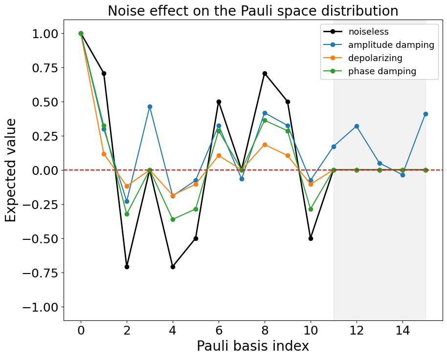
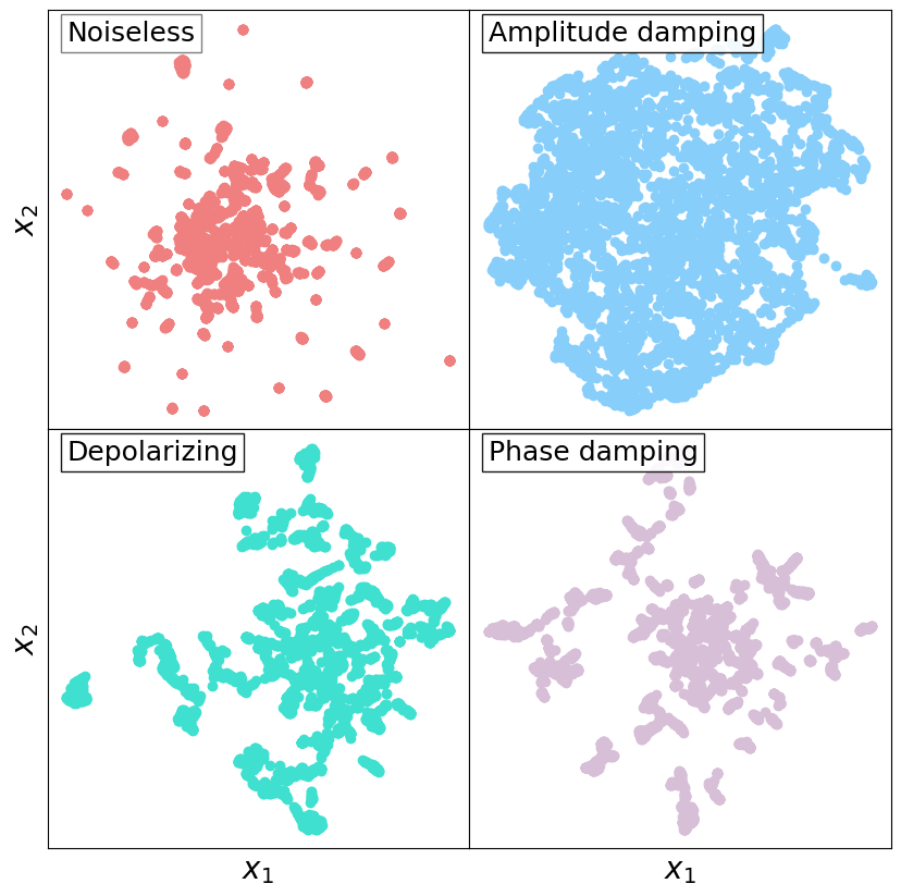
The previous theorem can be further illustrated with a two qubits toy model example. We design a QR with the three different quantum noise models and calculate the distribution of the Pauli coefficients at the end of the circuit. Figure 2 shows the outcomes of the measurements for a random circuit with 10 gates and an error rate of . We see that all noise models mitigate the non-zero coefficients. However, the shadowed area shows a region where the noiseless simulation (as well as the depolarizing and phase damping simulations) give zero expectation values. More importantly, the amplitude damping circuit has non-zero expectation values for the same operators, which means that this quantum channel has introduced non-zero terms in the Pauli distribution. For small error rates, the noisy quantum reservoirs provide better performance, since having amplitude damping noise produces a similar effect in terms of performance of the QRs as having more quantum gates in the circuit, as can be seen in Fig. 1 and also in Fig. 3 from Ref. Domingo et al. (2022). To better visualize this effect, we design 4000 random circuits and see how the final state fills the Pauli space. Since the Pauli space in the 2-qubit system is a 16-dimensional space, we use a dimensionality reduction technique called UMAP McInnes et al. (2020) to visualize the distribution in 2D. The results are shown in Fig. 3. We see that the amplitude damping channel fills the Pauli space faster than the other circuits, including the noiseless QR, thus confirming the hypothesis that the amplitude damping channel acts equivalently as having more quantum gates.
III Conclusions
In this paper, the effect on the QRC performance of three different paradigmatic noise models, effectively covering the most relevant and widely studied channels Nielsen and Chuang (2010); Tacla et al. (2023) affecting quantum devices, are evaluated. Contrary to common belief, we demonstrate that, under certain circumstances, noise, which constitutes the biggest challenge for quantum computing and QML, can be beneficial for quantum reservoir computing. Remarkably, we show that for error rates or state fidelities of at least , the presence of an amplitude damping channel renders better performance than noiseless QRs for the QML task at study, which consists of predicting the excited energy of the LiH molecule from its ground state. Moreover, our theoretical demonstration suggests that the benefits of amplitude damping noise will be also present in other tasks involving QRs, such as time series forecasting, which will be explored in future works. The performance of error mitigation techniques applied to QRs with different noise models will also be investigated in future studied. The effect of the amplitude damping channel is explained by analyzing the distribution in the Pauli space of the resulting density matrices after suffering the amplitude damping noise. This channel introduces additional non-zero coefficients in the Pauli space, which produces a similar effect as having more quantum gates in the original circuits. On the other hand, the depolarizing and phase damping channels only reduce the amplitude of the coefficients in the Pauli space, this producing poorer results. The depolarizing channel is the one that mitigates fastest these values, so our prescription is that its correction should be a priority. For this reason, error-correcting methods that target depolarizing noise Fitzek et al. (2020) should be employed in machine learning tasks involving the use of QRs.
IV Methods
subsectionQuantum Reservoir Computing
The idea of QRC lies in using a Hilbert space as an enhanced feature space of the input data. In this way, the feature space enhanced by quantum entangling operations are used to feed a classical machine learning model, which predicts the desired target. Consider a dataset , where are the input samples and the target outputs. The data samples are encoded as an -qubit quantum state . Then, a random unitary transformation is applied to extract features from the input data, resulting in the quantum state . The operator is sampled from a carefully selected family of operators, such that creates enough entanglement to generate useful transformations of the input data while being experimentally feasible. For this reason, the design of the reservoir is crucial for the optimal performance of the algorithm. In this work, the QRs are designed as random quantum circuits whose gates are chosen from a finite set. In a previous work Domingo et al. (2022), it was proven that the majorization principle Latorre and Martín-Delgado (2002), a relevant indicator of quantum circuit complexity Vallejos et al. (2021) for the NISQ era, serves as an indicator of performance for QRs. The G3={CNOT,H,T} family of random quantum circuits was found to provide an optimal design for QRs, where CNOT is the controlled-NOT gate, H stands for Hadamard, and T is the phase gate. For this reason, the G3 family is used to generate the reservoirs with a fixed number of gates.
After applying to the initial quantum state, the expected value of single-qubit Pauli observables is measured, providing the extracted features . Such features are fed to a classical machine learning algorithm. Even though complex machine learning models can be used, the QR should be able to extract valuable features so that a simple machine learning model can predict the targets . For this reason, a linear model is usually used to learn the output.
IV.1 Quantum machine learning task
In this work, QRs are used to predict the first excited electronic energy using only the associated ground state with energy for the LiH molecule. The ground state for the LiH Hamiltonian is calculated by exact diagonalization for different values of the internuclear distance a.u. The details of the ground state calculation are given in Ref Domingo et al. (2022). For this case, qubits are needed to describe the ground state, and QRs are used to predict the relative excited energy . The dataset is split into training and test sets, where the test set contains the 30% of the data a.u., and it is designed so that the QML algorithm has to extrapolate to new data samples.
IV.2 Noise models
The goal of this work is to study the effect of three noise models on the performance of the ML task, for different error probabilities and number of quantum gates. It is important to note that these models embody the overwhelming majority of noise types to which modern hardware is subjected to, this pointing out to the generality of our conclusions. The first noise model that we consider is the amplitude damping channel, which reproduces the effect of energy dissipation, that is, the loss of energy of a quantum state to its environment. It provides a model of the decay of an excited two-level atom due to the spontaneous emission of a photon with probability . The Kraus operators of this channel are given by
| (5) |
The operator transforms to , which corresponds to the process of losing energy to the environment. The operator leaves unchanged, but reduces the amplitude of . The quantum channel is thus
| (6) |
The second noise model is described by the phase damping channel, which models the loss of quantum information without loss of energy. The Kraus operators for the process are
| (7) |
and the quantum channel is then
| (8) | |||||
An alternative interpretation of the phase damping channel is that the state is left intact with probability , and a operator is applied with probability . The last noise model is described by the depolarizing channel. In this case, a Pauli error , or occurs with the same probability . The Kraus operators are
| (9) |
and the quantum channel is
| (10) |
The depolarizing channel transforms the state into the maximally mixed state with probability . Notice that the amplitude damping channel is the only one which is not unital, since it does not map the identity operator into itself. In general terms, it belongs to the kind of volume contracting environments in phase space with many generalizations that include the quantization of classical friction.
IV.3 Training process
The training steps of the algorithm are the following. First, the quantum circuit is initialized with the molecular ground state for a certain configuration . Next, a noisy quantum circuit with fixed number of gates is applied to . Then, we measure the local Pauli operators , where are the Pauli operators applied to the -th qubit, thus obtaining the vector
| (11) |
which provides the extracted information from the ground state. Recall that for a noisy state , the expectation value of an operator is given by . The vector is fed to a classical machine learning algorithm, in this case a ridge regression, which is a linear model with regularization. The optimal regularization parameter was , which reduces overfitting while maintaining optimal prediction capacity Domingo et al. (2022). The effect of the different noise channels in the algorithm performance is studied by varying the error probability . We perform 100 simulations for probabilities for each quantum channel, and compare the performance of the model with the noiseless simulation (). We also study how the number of quantum gates affects the performance of the reservoirs. We design circuits varying the number of gates from 25 to 215 in intervals of 10 gates. Also, we study the performance for large number of quantum gates, using 300, 500, 700 and 900 of them. All the simulations have been performed using Qiskit software Qiskit contributors (2023) via exact quantum circuit simulation with custom noise models (see Sect. VI).
V Data availability
The datasets generated and analysed during the current study are available in the GitHub repository, https://github.com/laiadc/Optimal_QRC_noise.
VI Code availability
The underlying code for this study is available in the Github repository and can be accessed via this link https://github.com/laiadc/Optimal_QRC_noise.
VII Competing interests
The authors declare no competing financial or non-financial interests.
VIII Author contributions
All authors developed the idea and the theory. LD performed the calculations and analyzed the data. All authors contributed to the discussions and interpretations of the results and wrote the manuscript.
IX Acknowledgments
The project that gave rise to these results received the support of a fellowship from “la Caixa” Foundation (ID 100010434). The fellowship code is LCF/BQ/DR20/11790028. This work has also been partially supported by the Spanish Ministry of Science, Innovation and Universities, Gobierno de España, under Contracts No. PID2021-122711NB-C21, ICMAT Severo Ochoa CEX2019-000904-S. The funders played no role in study design, data collection, analysis and interpretation of data, or the writing of this manuscript.
References
- Kreen and Zeilinger (2022) M. Kreen and A. Zeilinger, Proc. Natl. Acad. Sci. U.S.A. 117, 1910 (2022).
- Qiao et al. (2022) Z. Qiao, A. S. Christensen, M. Welborn, F. R. Manby, A. Anandkumar, and T. F. Miller III, Proc. Natl. Acad. Sci. U.S.A. 119, e2205221119 (2022).
- Arute et al. (2019) F. Arute, J. M. Martinis, and et al., Nature 574, 505 (2019).
- Harrow and Montanaro (2017) A. Harrow and A. Montanaro, Nature 549, 203 (2017).
- Cho (2019) A. Cho, “IBM casts doubt on Google’s claims of quantum supremacy,” https://www.science.org/content/article/ibm-casts-doubt-googles-claims-quantum-supremacy (2019).
- Liu et al. (2021) Y. A. Liu, X. L. Liu, F. N. Li, H. Fu, Y. Yang, J. Song, P. Zhao, Z. Wang, D. Peng, H. Chen, C. Guo, H. Huang, W. Wu, and D. Chen, in SC ’21: Proceedings of the International Conference for High Performance Computing, Networking, Storage and Analysis (Association for Computing Machinery, 2021).
- Zhong et al. (2019) H.-S. Zhong, L.-C. Peng, Y. Li, Y. Hu, W. Li, J. Qin, D. Wu, W. Zhang, H. Li, L. Zhang, Z. Wang, L. You, X. Jiang, L. Li, N.-L. Liu, J. P. Dowling, C.-Y. Lu, and J.-W. Pan, Science Bulletin 64, 511 (2019).
- Zhao and et al. (2022) Y. Zhao and et al., Phys. Rev. Lett. 129, 030501 (2022).
- Ugwuishiwu et al. (2022) C. Ugwuishiwu, O. Ugochukwu, O. Ukwueze, and P. Ogbobe, Int. J. Sci. Technol. Res. 11, 1 (2022).
- Takagi et al. (2022) R. Takagi, S. Endo, S. Minagawa, and M. Gu, npj Quantum Inf. 8, 114 (2022).
- Guo and Yang (2022) Y. Guo and S. Yang, PRX Quantum 3, 040313 (2022).
- AI (2023) G. Q. AI, Nature 614, 676 (2023).
- Mujal et al. (2021) P. Mujal, R. Martínez-Peña, J. Nokkala, J. García-Beni, G. Giorgi, M. Soriano, and R. Zambrini, Adv. Quantum Technol. 4, 2100027 (2021).
- Fujii and Nakajima (2017) K. Fujii and K. Nakajima, Phys. Rev. Appl. 8, 024030 (2017).
- Nakajima et al. (2019) K. Nakajima, K. Fujii, M. Negoro, K. Mitarai, and M. Kitagawa, Phys. Rev. Appl. 11, 034021 (2019).
- Kutvonen et al. (2020) A. Kutvonen, K. Fujii, and T. Sagawa, Scientific Reports 10, 14687 (2020).
- Chen et al. (2020) J. Chen, H. I. Nurdin, and N. Yamamoto, Phys. Rev. Appl. 14, 024065 (2020).
- Martínez-Peña et al. (2020) R. Martínez-Peña, J. Nokkala, G. L. Giorgi, and J. Amato-Grill, Cognitive Computation 12, 1 (2020).
- Martínez-Peña et al. (2021) R. Martínez-Peña, G. L. Giorgi, J. Nokkala, M. C. Soriano, and R. Zambrini, Phys. Rev. Lett. 127, 100502 (2021).
- Ghosh et al. (2019a) S. Ghosh, A. Opala, M. Matuszewski, T. Paterek, and T. C. H. Liew, npj Quantum Inf. 5, 35 (2019a).
- Ghosh et al. (2021) S. Ghosh, A. Opala, M. Matuszewski, T. Paterek, and T. C. H. Liew, IEEE Transactions on Neural Networks and Learning Systems 32, 3148 (2021).
- Ghosh et al. (2019b) S. Ghosh, T. Paterek, and T. C. H. Liew, Phys. Rev. Lett. 123, 260404 (2019b).
- Krisnanda et al. (2021) T. Krisnanda, S. Ghosh, T. Paterek, and T. C. Liew, Neural Networks 136, 141 (2021).
- Domingo et al. (2022) L. Domingo, G. Carlo, and F. Borondo, Phys. Rev. E 106, L043301 (2022).
- Liu et al. (2022) J. Liu, F. Wilde, A. A. Mele, L. Jiang, and J. Eisert, “Noise can be helpful for variational quantum algorithms,” (2022), arXiv:quant-ph/2210.06723 .
- Xia and Kais (2018) R. Xia and S. Kais, Nat. Commun. 9 (2018), 10.1038/s41467-018-06598-z.
- Kawai and Nakagawa (2020) H. Kawai and Y. Nakagawa, Mach. Learn.: Sci. Technol. 1, 045027 (2020).
- Alam and Ghosh (2022) M. M. Alam and S. Ghosh, Frontiers in Physics 9, 755139 (2022).
- Tüysüz et al. (2021) C. Tüysüz, C. Rieger, K. Novotny, T. Drielsma, and M. Winn, Quantum Machine Intelligence 3, 29 (2021).
- Schatzki et al. (2021) L. Schatzki, A. Arrasmith, P. J. Coles, and M. Cerezo, (2021), arXiv:2109.03400 [quant-ph] .
- McInnes et al. (2020) L. McInnes, J. Healy, and J. Melville, “UMAP: uniform manifold approximation and projection for dimension reduction,” (2020), arXiv:1802.03426 .
- Nielsen and Chuang (2010) M. A. Nielsen and I. L. Chuang, Quantum computation and quantum information (Cambridge university press, 2010).
- Tacla et al. (2023) A. B. Tacla, N. M. O’Neill, G. G. Carlo, F. de Melo, and R. O. Vallejos, “Majorization-based benchmark of the complexity of quantum processors,” (2023), arXiv:2304.04894 [quant-ph] .
- Fitzek et al. (2020) D. Fitzek, M. Eliasson, A. F. Kockum, and M. Granath, Phys. Rev. Res. 2, 023230 (2020).
- Latorre and Martín-Delgado (2002) J. I. Latorre and M. A. Martín-Delgado, Phys. Rev. A 66, 022305 (2002).
- Vallejos et al. (2021) R. Vallejos, F. de Melo, and G. G. Carlo, Phys. Rev. A 104, 012602 (2021).
- Qiskit contributors (2023) Qiskit contributors, “Qiskit: An open-source framework for quantum computing,” (2023).