AutoDDL: Automatic Distributed Deep Learning with Asymptotically Optimal Communication

Abstract

Recent advances in deep learning base on growing model sizes and the necessary scaling of compute power. Training such large-scale models requires an intricate combination of data-, operator-, and pipeline parallelism in complex distributed systems. We show how to use OneFlow’s Split, Broadcast, and Partial Sum (SBP) tensor formulations to enable new distributed training methods with asymptotically optimal communication overheads. Using these insights, we develop AutoDDL, a distributed training framework that combines an exhaustive performance model and automated configuration search to find distributions with near-optimal communication overheads. We conduct evaluations on Multi-Node-Single-GPU and Multi-Node-Multi-GPU machines using different models, including VGG and Transformer. Compared to expert-optimized implementations, AutoDDL reduces the end-to-end training time by up to 31.1% and 10% for Transformer and up to 17.7% and 71.5% for VGG on the two different systems, respectively.

1 Introduction

The quickly growing model size advances the continued success of deep learning [21]. The large-scale deep learning models require tremendous hardware resources, making distributed training on parallel machines necessary. However, training these large models is both time-consuming and expensive. Taking training GPT-3 (with 175 billion parameters) [5] as an example, it took seven months on 512 GPUs and costs millions of dollars. Therefore, an efficient parallelization scheme is of great importance for large-scale model training.

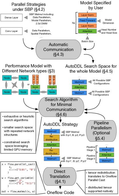
Figure 1: The workflow of AutoDDL.

Data, operator, and pipeline parallelizations are three commonly used methods for distributed training. Their communication overheads are the main bottleneck in distributed training [17]. Even just deciding on exact decomposition of this three dimensional parallelism is a daunting effort [30, 11]. Due to this complexity, no comprehensive scheme uses communication-avoiding techniques [23, 6] that can lead to significant reduction in communication volume. Thus, communication-avoiding automatic DNN training is not a solved problem since (1) the space of all possible parallel training strategies is not adequately defined and sub-optimal in current works [24, 44, 19, 31], (2) Finding a good strategy in a vast space can be challenging, and (3) implementing parallel strategies without the support for automatic code generation requires a lot of effort.

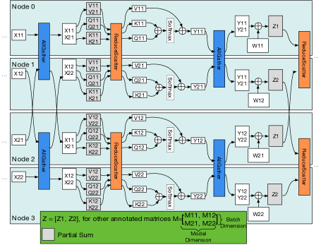
Figure 2: An example strategy for the self-attention layer in AutoDDL search space with four compute nodes (communication drawn only for the forward path, emitting the data-parallel dimension). One can compare the figure with Megatron’s model parallelism (MP) since both can be easily combined with data parallelism. Megatron’s MP replicates the input matrix X and splits the model weights W in one dimension. The AutoDDL strategy additionally splits the input X along the model dimension and splits the weights along both dimensions.

To handle the challenges above, we propose an Automatic framework for Distributed Deep Learning (AutoDDL). The workflow of AutoDDL is shown in Figure 1. We created a more extensive search space for parallel DNN training schemes inspired by the SBP abstraction of the previous work Oneflow [43]. Unlike previous distributed deep learning approaches [44, 19, 31], our search space has an additional Partial tensor state to enable communication-avoiding algorithms. We prove that this new search space includes asymptotically communication-optimal strategies with suited strategies adapted to the different neural network layers similar to 2.5D distributed matrix multiplication (DMM) algorithms  [38, 8, 23], i.e., using p compute nodes and matrix size $n^{2}$, both the communication and memory costs are in $\Theta\left(\frac{n^{2}}{p^{2/3}}\right)$. However, many works on distributed deep learning, like Data Parallelism [3], Megatron [31], Flexflow [19], and Alpa [44], use communication sub-optimal distributed algorithms. For instance, Megatron has $\mathcal{O}\left(\frac{n^{2}}{p^{1/2}}\right)$ communication costs and $\mathcal{O}\left(\frac{n^{2}}{p^{1/2}}\right)$ memory consumption.

Figure 2 shows AutoDDL’s decomposition for a transformer model. We see that compared with Megatron’s model parallelism [31], the AutoDDL strategy exploits more parallel dimensions and splits the tensors more fine-grained to obtain the asymptotic advantage.

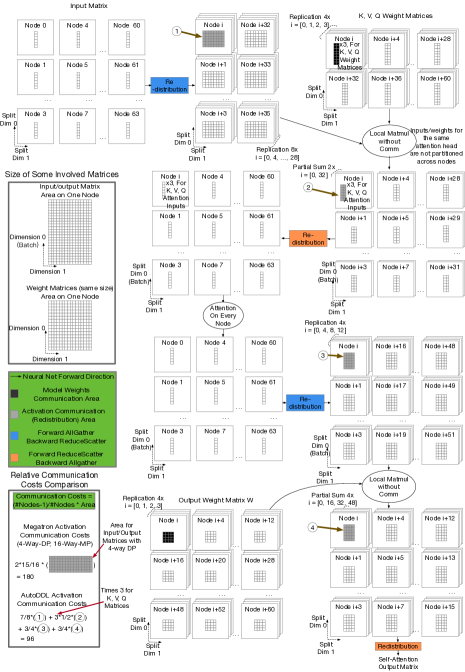
Figure 3: Parallel strategies for one Attention layer in our actual experiment using 64 nodes. The model is large, so it needs more than 16 nodes to carry the model weights. The best Megatron strategy is 4-way data parallel (DP) and a 16-way model parallel (MP). Megatron’s MP communicates the input and output matrices using 16 nodes with the area divided by 4. AutoDDL has similar model weights communication costs (for gradient synchronization in the backward path) and less intermediate activation communication costs (shown in Figure) than Megatron.

Supported Models Asymptotically Optimal Strategy Search Cost Ease of Adaptation Data Parallel [25] Models fit in memory No Guarantee N/A Easy Operator Parallel [22, 40] All No Guarantee N/A Hard Megatron [31] Transformers No Guarantee N/A Medium Summa [41] Matmul For DMM Communication N/A Medium Flexflow [19] All No Guarantee High Easy Alpa [44] All No Guarantee High Easy AutoDDL All For DMM Communication Low Easy

Table 1: Comparison of distributed deep learning methods. We analyze four aspects: supported models, possibility of achieving asymptotically optimal communication, cost of strategy search, and ease of adaptation: Summa and AutoDDL obtain the asymptotically optimal communication for DMM, whereas approaches do not. AutoDDL searches strategies on CPUs (lower overheads). Data parallelism and the automatic frameworks can be adapted with less user effort. The user must determine the 2D node mesh for Summa and Megatron, whereas operator parallelism must be designed for specific models.

With these theoretical insights, our search space can contain parallel execution plans with a lower communication overhead than previous works. Figure 3 shows an detailed strategy selected by AutoDDL for an attention layer computed on 64 nodes. The AutoDDL strategy has similar communication costs for weight gradient synchronization as Megatron. However, intermediate activation communication costs are nearly halved: the relative communication ratio is 96:180, as shown in Figure 3. The illustrated transformer has a model size of 8,192, and the batch size and sequence length are 1,024 (numbers takes from the Megatron paper [31]). The intermediate activation communication is 3.75 billion elements per attention layer for Megatron (15 GB). AutoDDL has reduced the communication to 2 billion elements (8 GB).

In order to find a communication-reducing parallel strategy in the search space, a performance model is built for AutoDDL: it accurately ranks the communication overhead of different parallel execution plans. With the help of the performance model, we show that one can find a good strategy quickly via exhaustive search or heuristic algorithms. The OneFlow deep learning framework [43] adapts the SBP annotation and communication mechanisms for distributed tensors natively, different from other deep learning frameworks such as TensorFlow [1] and PyTorch [33]. Hence, the AutoDDL selected execution plan directly translates to tensor annotations and redistribution primitives in OneFlow. Overall, AutoDDL enables both high performance and high productivity. Our main contributions are:

• AutoDDL supports a novel search space that can achieve asymptotically optimal communication and adapts different parallel execution schemes to different layers according to their sizes. The expanded search space is essential for reducing communication costs that existing frameworks do not support.

• We establish a performance model that successfully guides the search for the parallel execution plan with low communication overhead. It takes only minutes to find a performant parallel execution scheme on a personal laptop.

• We integrate OneFlow into the workflow of AutoDDL, which enables the automatic implementation of various parallel execution plans via the SBP abstraction.

• We are the first to show that an automated parallel strategy search can outperform manually designed and optimized parallel deep learning strategies like Megatron by up to 10% and 31.1% on Google Cloud and the Piz Daint supercomputer, respectively.

Experimental results show that AutoDDL can save the end-to-end training time for Transformer models by up to 31.1% on GPU clusters equipped with high-performance interconnected networks. The estimated cost to train GPT-3 is more than $4.6m. This implies that AutoDDL can save about $1.4m when training such a large model.

2 Background and Related Work

Data parallelism [25, 37] is the most widely-used distributed deep learning approach. Operator parallelism [22, 9, 10] splits specific operators and communicates the model’s intermediate result for result consistency. Megatron [31] combines data and operator parallelism and is expert-designed primarily for the Transformer language model. In this paper, we hand-tune Megatron to the best performance and use it as an experimental baseline. The deep learning framework OneFlow [43] has proposed an SBP abstraction that can conveniently express data- operator- and their hybrid parallelism. The SBP abstraction is presented in detail in Section 4. AutoDDL builds its automatic strategy search upon the SBP abstraction.

Another line of research is to apply ideas from the traditional HPC community. The Summa algorithm for DMM, well-known for its memory-saving nature, has been applied to deep learning for memory constraint cases [12, 4]. We implement the Summa version from Optimus [4] in OneFlow as another experimental baseline.

There are operator parallelisms specifically for convolution layers such as spatial [9], channel, and filter parallelism [10]. Especially, Kahira et al. have built a network communication model that determines the best combination for the convolution parallel approaches [20], which is similar to our performance model (Section 3.2).

There are other orthogonal approaches to AutoDDL’s SBP parallel strategies. Pipeline parallelism [28, 42, 18, 26, 13, 27, 29] explores inter-layer parallelism and can suffer from load balancing, idleness, or staleness issues. Our experiments show that AutoDDL can provide notable benefits against Megatron when pipeline parallelism is enabled for both. AutoDDL enables gradient accumulation [7] to save memory, as it has a small influence on performance with a lot of memory saving.

At a higher level, other automatic DNN training frameworks have been proposed in the literature. FlexFlow [19] uses MCMC [2] to determine a suitable placement and parallel strategy for each operator in a DNN. Alpa [44] has recently been proposed to search for a suitable strategy using compilation techniques. However, their limited search spaces do not include asymptotically communication optimal algorithms and have not shown performance improvements toward expert-designed Megatron. Flexflow and Alpa simulate strategy performance on real GPUs, whereas our search is based on an accurate performance model and entirely done using CPUs. For complex models and vast search spaces, performance model-based search can have advantages in its fast speed and no requirement for GPUs.

Our work is the first to combine automatic strategy search and asymptotic communication-optimal algorithms and has successfully shown performance benefits against Megatron (the expert-optimized implementation). Table 1 summarizes the main distinguishing factors of AutoDDL.

3 Communication Performance Model

Collective communications are core for distributed deep neural network training. The most commonly-used collective is AllReduce [34]: The weight gradients need to synchronize using AllReduce in data parallelism. We also need collective operations like AllGather, ReduceScatter, and AlltoAll for AutoDDL. In the literature, Collective performance has been modeled using the alpha-beta model to derive DMM algorithms  [35].

3.1 Collective Performance based on the Alpha-Beta Model

The alpha-beta model is a well-known model for simulating network communication time. $\alpha$ is the network latency, and $\beta$ is the inverse network bandwidth. Communicating a single n-byte message takes $\alpha+n\beta$ time. Some collectives, like ReduceScatter and AllReduce, involve computation. However, the computation part is omitted from our analysis since it is small and can be overlapped with communication. We use the alpha-beta model to facilitate the costs of ring-based collective communications, similar to Nguyen et al. [32], since 1) Ring-AllReduce is widely adapted in deep learning training, and 2) the ring-based algorithms are bandwidth optimal. Large messages are often communicated in large-scale model training, making bandwidth-optimal algorithms more desirable. The costs for the collectives are summarized in Table 2.

Collective	Communication Complexity
AllReduce	$\left\lceil{2p-1}\right\rceil\alpha+2\left\lceil\frac{p-1}{p}\right\rceil n\beta$
AllGather/ReduceScatter	$\left\lceil{p-1}\right\rceil\alpha+\left\lceil\frac{p-1}{p}\right\rceil n\beta$
AlltoAll	$\left\lceil{p-1}\right\rceil\alpha+\left\lceil\frac{p-1}{p}\right\rceil n\beta$

Table 2: Communication Complexity of Bandwidth-Optimal MPI Collectives. N is the message size for ReduceScatter’s inputs and other collectives’ outputs.

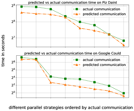
Figure 4: Actual communication time versus the performance model’s prediction for eight different parallel strategies of a Transformer neural network. The parallel strategies are ranked by actual communication costs on the x-axis.

3.2 Inferring Network Parameters on Real World Systems

Instead of using the theoretical peak latency and bandwidth reported by hardware manufacturers, we build a more practical alpha-beta model for collective communication by inferring the $\alpha$ and $\beta$ parameters in an actual environment.

In this paper, we build communication models for the Piz Daint Supercomputer, a Multi-Node-Single-GPU environment. And we establish a similar model for the Google Cloud Platform Network and NVlink for a Multi-Node-Multi-GPU system. The configurations of these Platforms are detailed in Section 5. The actual runtime for four collectives (AllReduce, AllGather, AlltoAll, and ReduceScatter) with various massage sizes and various numbers of devices are collected 100 times each. According to Table 2, the collected data can be summarized as a linear system in $\alpha$ and $\beta$ for each network. Then, we infer the parameters using the least square method.

3.3 Ranking of different parallel strategies via the communication model

The purpose of the communication model is to rank different parallel strategies reasonably so one can select a strategy with low communication costs. Each parallel strategy of a DNN in our AutoDDL space can be seen as a chain of computation and collective communications (detailed in Section 4), where the communication part can be modeled using the alpha-beta model. Figure 4 shows the same Transformer model’s actual communication costs versus the performance model’s prediction on Piz Daint and Google Cloud. We run the experiments on 32 single-GPU nodes on Piz Daint and 2 eight-GPU nodes on Google Cloud. We put the parallel strategies in descending order of measured communication costs, and one can see in Figure 4 that the performance model is accurate enough to capture the ordering on both platforms.

4 The AutoDDL Strategy Search

The most critical aspect of AutoDDL is the automatic selection of distributed deep neural network training strategies. We first define the AutoDDL search space: a space that is based on OneFlow’s native SBP interface and abstraction. The SBP notation will be explained in Section 4.1, and the AutoDDL space in 4.2. Primarily, we focus on communication avoiding aspects of performance while preserving the total compute cost. It is shown in Section 4.3 that the asymptotically communication-optimal strategy is contained in our search space. Sections 4.4 and 4.5 focus on an efficient search for an end-to-end DNN.

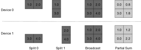
Figure 5: Basic SBP of a 2d tensor on a group of two devices. A 2d tensor can be in Split 0 and Split 1 (split along dimensions 0 and 1), Broadcast (Replication), and Partial Sum states. Bright color represents a partial sum: the elements must be summed to retrieve the original tensor.

4.1 OneFlow’s native support for SBP

SBP is an abstraction OneFlow provides for describing distributed tensors. An n-dimensional tensor can be a partial sum, replicated (broadcasted), and split along all n dimensions on different devices (see Figure 5).

⬇

1#initialising a 2d tensor w

2#w has distribution (S1:2, S0:3, B:4)

3#device_id is a list of devices

4import oneflow

5distribution = ["S(1)", "S(0)", "B"]

6

7with oneflow.scope.placement("gpu", device_id, (2, 3, 4)):

8 w = oneflow.get_variable(

9 name="2d_tensor",

10 shape=(6, 4),

11 dtype=oneflow.float,

12 trainable=True,

13 parallel_distribution=distribution,

14 )

Listing 1: OneFlow SBP Initialization Example

Compared to the famous GShard [24] API, Oneflow’s Broadcast State corresponds to the Replicate state in GShard, and Oneflow’s Split States generalize the Split and Shard states in GShard. The SBP abstraction has one more Partial Sum state P, which is the key to a more extensive search space with potentially better parallel strategies.

The OneFlow deep learning framework natively provides distributed tensor initialization and tensor redistribution. With 24 devices in total, Listing 1 shows the code for initializing a 6*4 tensor, whose first and second dimensions are split on three and two devices, respectively. The whole 6*4 tensor is then replicated on the remaining four devices. Listing 2 is an actual code example for tensor redistribution, and the code is used for one of our CNN training strategies. If we have a heterogeneous network like the multi-node-multi-GPU setting, the GPUs on the same compute node can be identified as we provide a list of device/GPU IDs to OneFlow.

⬇

1# a tensor redistribution example

2#device_id is a list of devices

3import oneflow

4

5with oneflow.scope.placement("gpu", device_id, (8, 4)):

6 #previous x has distribution (P:4, S1:8)

7 x = oneflow.hierarchical_parallel_cast(x,parallel_distribution=["S(1)", "S(1)"])

8

9with oneflow.scope.placement("gpu",device_id):

10 x = oneflow.hierarchical_parallel_cast(x,parallel_distribution=["S(1)"])

11#now x has distribution (S1:32)

Listing 2: OneFlow Boxing Example

One advantage of AutoDDL is that it can directly use OneFlow’s distributed initialization and redistribution codes, similar to Listing 1 and Listing 2. Any distributed strategy selected by AutoDDL can be easily implemented with the OneFlow API. Programmers no longer need to place and communicate distributed tensors manually.

4.2 Parallel Strategies

The SBP tensor distribution enables the description of a search space for distributed DNN training strategies. The strategies are intra-layer, meaning each layer can have a different SBP distribution. Operations, such as activation functions, dropouts, layer normalization, and self-attentions, require the input to be evenly split. Hence, we constrain every layer’s output in the AutoDDL search space to be split, i.e., S distributions in SBP. Some operations like self-attention put additional restrictions on the input split dimensions, which AutoDDL addresses automatically.

4.2.1 General SBP Layer

Generally, an engineer can implement parallel execution strategies for any operation as a chain of computation and SBP tensor redistributions in the AutoDDL search space. AutoDDL can simulate all the redistribution overheads and find a near-best strategy with little communication. Performance engineers can add new communication patterns beyond SBP, like halo exchange for CNNs [9] or looped rank-k updates for Summa [41], and invent new layers in AutoDDL. For example, our Summa baseline is implemented in OneFlow with specific SBP input and output tensor distributions. The newly invented layers can be included in our automatic search framework as long as an accurate performance model and their input/output SBP distributions are provided.

We will explain our SBP matrix multiplication in Section 4.2.2. Other strategies for convolution [9, 10] and many other layers can be implemented under this framework for a larger AutoDDL search space and potentially a more significant performance boost.

4.2.2 SBP Matrix Multiplication

Matrix multiplication (Matmul) is an essential operation in deep learning. Our SBP matrix multiplication algorithm follows: The input matrix $I$, weight matrix $W$, and the output matrix $O$ are all two-dimensional tensors. We can assume $p=p_{0}*p_{1}*p_{2}$ devices are available. For matrix multiplication $IW=O$, If the input matrix I has distribution (S0: $p_{0}$, B: $p_{1}$, S1: $p_{2}$) and the initialized weight matrix W has distribution (B: $p_{0}$, S1: $p_{1}$, S0: $p_{2}$). Then, the matrix multiplication is performed locally on each device. The resulting output matrix O will have an SBP distribution (S0: $p_{0}$, S1: $p_{1}$, P: $p_{2}$). Figure 6 shows the SBP Matmul with an actual example. Notice that if p1 and p2 are both 1, the algorithm is simply data parallelism.

The above computation assumes the SBP matrix multiplication has its input and output in the correct SBP distribution. However, data redistribution (explicit SBP layout changes that translate to proper collective communication patterns under the hood) is inevitable to chain different layers into a DNN. The combination happens automatically in AutoDDL and is explained in Section 4.3.

4.2.3 Multi-Node-Multi-GPU Strategies

The tensor distributions and strategies in the Multi-Node-Multi-GPU case are very similar. Instead of using numbers to denote SBP, we use tuples to represent the number of nodes and the number of GPUs per node for each SBP dimension. For example, the input matrix for an SBP matmul is of the form (S0: $(p_{0},p_{0}\textquoteright)$, B: $(p_{1},p_{1}\textquoteright)$, S1: $(p_{2},p_{2}\textquoteright)$) for a system with $p=p_{1}*p_{2}*p_{3}$ nodes and each node with $p\textquoteright=p_{1}\textquoteright*p_{2}\textquoteright*p_{3}\textquoteright$ GPUs per node. If a communication only involves intra-node GPUs (the first entry in the corresponding tuple is 1), the performance model uses the intra-node NVlink bandwidth. Otherwise, the communication is deemed to be on the slower inter-node network.

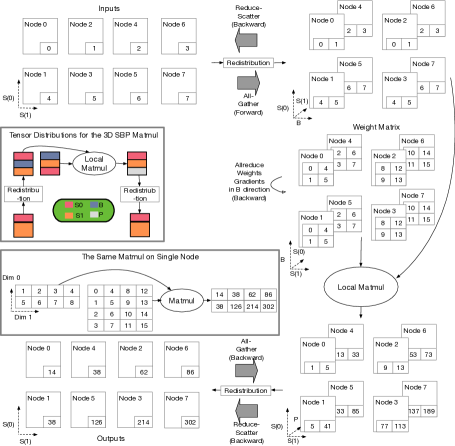
Figure 6: shows a 3d SBP DMM example. The tensor distributions are shown in color, and the same matrix multiplication on a single node is included for comparison.

4.3 Automatic Communication

For an SBP layer, we first define the input SBP distribution and constrain its output distribution. Then, our AutoDDL framework can automatically conduct the data redistribution between two consecutive layers. Let us consider an example of SBP matrix multiplication:

For any consecutive SBP matrix multiplication operations $M_{i}$ and $M_{i+1}$, where $M_{i}$’s output, after going through operations like activation function without changes in its distribution, becomes $M_{i+1}$’s input. $M_{i}$’s output originally has SBP distribution (S0: $p_{0}$, S1: $p_{1}$, P: $p_{2}$) and $M_{i+1}$ needs input SBP distribution (S0: $p_{0}^{\prime}$, B: $p_{1}^{\prime}$, S1: $p_{2}^{\prime}$) (see 4.2.2). If $p_{0}=p_{0}^{\prime}$, the required tensor redistribution path is (S0: $p_{0}$, S1: $p_{1}$, P: $p_{2}$) -> (S0: $p_{0}$, S1: $p_{1}*p_{2}$) -> (S0: $p_{0}^{\prime}$, B: $p_{1}^{\prime}$, S1: $p_{2}^{\prime}$), where the appropriate redistributions denoted by "->" translate to collective communications in the forward/backward path automatically. This special case is shown in Figure 6. The other special case with $p_{1}=p_{2}^{\prime}$ is analog. The redistribution communications for these special cases are ReduceScatter and Allgather collectives in the forward path and Allgather and ReduceScatter in the backward path. For general cases where $p_{0}!=p_{0}^{\prime}$ and $p_{1}!=p_{2}^{\prime}$, the required change of data distributions is (S0: $p_{0}$, S1: $p_{1}$, P: $p_{2}$) -> (S0: $p_{0}$, S1: $p_{1}*p_{2}$) -> (S0: $p_{0}^{\prime}$, S1: $p_{1}\textquoteright*p_{2}^{\prime}$) -> (S0: $p_{0}^{\prime}$, B: $p_{1}^{\prime}$, S1: $p_{2}^{\prime}$). Additional AlltoAll collectives are required for (S0: $p_{0}$, S1: $p_{1}*p_{2}$) -> (S0: $p_{0}\textquoteright$, S1 :$p_{1}\textquoteright*p_{2}\textquoteright$).

4.4 Communication Cost Analysis

After the definition and combination of different layers with different parallel strategies, the overall communication for a DNN can be decoupled into a sequence of collectives. One can analyze each collective operation according to Section 3.

4.4.1 Two Sources of Communication

The communication for any algorithms in the AutoDDL search space happens twofold. The first source of communication overhead is weight gradient synchronization: if any weight matrix W is replicated, it gets only a portion of the gradients in the backward path, and an AllReduce is required for accumulating the gradient information. The second source is the data redistribution for SBP layout transformations, as discussed in Section 4.3.

4.4.2 Asymptotic Communication for SBP Matmul

A well-known fact is that the communication lower bound for a n*n matrix with p devices consuming $\Theta(\frac{n^{2}}{p^{2/3}})$ memory per device is $\mathcal{O}(\frac{n^{2}}{p^{2/3}})$ [36]. Figure 6 shows an example of a complete 3d SBP matrix multiplication. All the involved tensors’ local volume is divided by no less than $\frac{p}{\max(p_{1},p_{2},p_{3})}$ (divided by p and replicated by deep granite and white color times in the data distribution example in Figure 6). If we select $p_{1}$, $p_{2}$, $p_{3}$ (all two in the example figure) to be in $\mathcal{O}(p^{1/3})$, both the communication volume and memory occupation is in $\Theta(\frac{n^{2}}{p^{2/3}})$. This example shows that the asymptotically optimal matrix multiplication lies in our search space.

4.5 Searching An End-to-End Strategy

The AutoDDL search space can include all possible SBP parallel strategies for each layer. Hence, the search space can often be huge, and we introduce several techniques for shrinking the space.

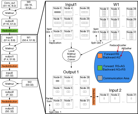
Figure 7: AutoDDL for the last three dense layers of vgg13 on 32 GPUs. The second matrix multiplication and the tensor redistributions are shown in detail. Notice that the weight matrices are not replicated. Hence the weight gradients do not need to be summed up using AllReduce in the backward path.

4.5.1 Limit the Search Space for Repeated Layers

The search space grows exponentially with the number of layers. Exhaustive search may be feasible for VGG models with three dense layers but prohibitively expensive for GPT models with more than 30 attention and dense layers. Notably, the same neural network architecture is repeated for many neural networks, including GPT models. Hence, we restrict the repeated layers to identical SBP distributions, dramatically reducing the strategy search time.

4.5.2 Leveraging Memory Limitations

Different strategies have different implications for memory consumption. Many strategies cause out-of-memory (OOM) errors. Thankfully, the OneFlow framework can determine the exact memory usage on a single laptop before actually training on GPUs. Since we used gradient accumulation for all the experiments, the main bottleneck for memory was the model parameters and its optimizer states. As explained in previous sections, the weight matrix has a distribution of (B: p0, S1: p1, S0: p2). The weights are replicated p0 times, causing memory issues. Therefore, we restrict p0 for each SBP Matmul below a certain threshold and search for the best strategy under restriction. Memory tests are required and done manually for the Megatron baselines.

4.5.3 An End-to-End DNN Example

Figure 7 shows an actual example of the VGG network’s last three dense layers. The convolution operations work in a data-parallel manner with (S0: p) for inputs and outputs. The selected strategy has zero weight gradient synchronizations and little data redistribution communication. This strategy is reasonable since model dimensions are many times larger than the batch size for VGG, and avoiding weight gradient synchronization benefits the overall communication.

4.6 Heuristic Search Algorithms

Even though our AutoDDL search happens on a single CPU node with performance model simulations, the search space can still be huge for complex models with many different layers trained on thousands of large-scale. The exhaustive search must iterate over the whole search space and can be slow. This subsection investigates two heuristic algorithms proposed in the literature: the metropolis-hastings algorithm [15] and coordinates descent [39]. We compare them with the random and exhaustive search on a 4-layer MLP example. The experiments show that the heuristic algorithms can be orders of magnitude faster with minimal performance loss. With the help of existing heuristic algorithms, our AutoDDL strategy search can scale to more complex models on more compute nodes at a low runtime cost.

The Metropolis-Hastings Algorithm. We define each strategy’s sampling probability as

$$P(S)\propto exp(-\beta\cdot Cost(S))$$

The term $\beta$ is a chosen constant. The algorithm starts with an initial strategy and proposes a new strategy each time, with only one layer randomly changing its SBP distribution. The metropolis-hastings algorithm accepts the proposed strategy with the probability

$$min(1,P(S_{new})/P(S_{old}))$$

The process is repeated indefinitely, creating a chain of strategies. The treatment is similar to Flexflow’s MCMC simulation [19]. A new strategy is accepted if it costs less than the current one. Suppose a new strategy has a higher cost, its acceptance probability decrease exponentially with $Cost(S_{new})-Cost(S_{old})$. Intuitively, the algorithm accepts a lower-cost strategy greedily to minimize the costs and a higher-cost strategy with a small probability so that a local minimum can be escaped.

The Coordinates Descent Algorithm. The coordinates descent algorithm starts with an initial strategy, and it iteratively changes and optimizes every layer’s SBP distribution: a strategy S for a neural network with L layers can be written as $S=[s_{j}]_{j=0}^{L}$ with $s_{j}$ the strategy for layer j. One update step of coordinate descent is that for every layer i

$$S[i]=\operatorname*{arg\,min}_{s_{i}}Cost([s_{j}]_{j=0}^{L})$$

The distribution of the current layer is chosen to minimize the total costs, with the other layers’ distributions unchanged. Coordinate Descent has been shown to explore a large discrete search space efficiently [14]. Our version of the algorithm decreases the cost monotonically for each update step via greedy line searches along single layers’ strategy space. Once a fixed point is reached, we record the best strategy and start with a new initial guess. So the algorithm can escape a local minimum by re-initializing the starting point.

Evaluation. We compare the metropolis-hastings and the coordinate descent algorithms with the exhaustive and random search. With a limited time budget, the algorithms should select a strategy for a 4-layer MLP with dimensions 32,768, 16,384, 4,096, 2,048, and 512. We have not tested larger models since the exhaustive search would take too long. The test environment is Intel® Xeon® E5-2695 v4 @ 2.10GHz CPU on the Piz Daint Supercomputer. Figure 8 shows the algorithms’ performance simulating 128 and 4,096 compute nodes. Coordinates descent selects the best strategy in both settings, and the metropolis-hastings method performs second best. Both heuristic algorithms can find a near-optimal strategy in 2-4 orders of magnitude less runtime than the exhaustive search. However, the random search cannot find a strategy close to optimal using the same runtime budget.

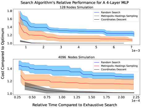
Figure 8: Performance comparison of random search, exhaustive search, metropolis-hastings, and coordinates descent algorithms. The shaded area shows the 90% confidence interval over ten runs. The communication cost relative to optimum is plotted on the y-axis, and the relative time to exhaustive search is plotted on the x-axis. Exhaustive search is slow but achieves the optimum (1 on the y-axis).

5 Experiments

We evaluate our near-optimal distributed training strategy from the AutoDDL space on two Deep neural network architectures on Multi-node Single-GPU and Multi-node Multi-GPU settings. The performance is compared against data parallelism, Megatron [31], and Summa [41] algorithm.

Megatron and Summa are 2d algorithms, and their 2d distributions of the devices must be determined. We hand-optimize the best 2d device mesh for the baselines on the Multi-node Single-GPU environment. For the Multi-node Multi-GPU, we put communication for intermediate results on NVLink as in [31], so it enjoys high bandwidth and low latency within compute nodes. The communication for model weights is inevitably placed on the network across nodes. All experiments are repeated ten times, and the error bars show the 99% confidence interval around the mean, as suggested in [16].

5.1 Experiment Configurations

5.1.1 The VGG Model

We use VGG13 throughout the experiments and increase the batch size with the number of GPUs. Memory is not a limiting factor for most convolution neural networks, including VGG13, so no gradient accumulation is applied.

The convolution layers in VGG13 comprise most of the computation but only a tiny portion of the weights. Hence, data parallelism is suitable for convolution layers. The last three dense layers are the leading cause of communication, and we apply the best AutoDDL strategy for these three dense layers. After the outputs of the convolution layers have been transformed to the correct distributions, a Megatron-like 2d algorithm can be applied to the last three dense layers.

Although the Summa algorithm alleviates memory redundancy issues, it does not provide the best performance for non-memory-constrained cases like CNN. Our empirical evaluations show that Summa is an order of magnitude slower than other methods on VGG. Hence, we omit Summa in the VGG experiment plots.

5.1.2 The Transformer Model

Transformer has many parameters that control its size: the model dimension, number of attention heads, and attention head dimension. The model sizes we chose are taken from the Megatron-lm paper [31].

The batch size for language model pre-training is usually in the order of millions of tokens, and we use gradient accumulation to leverage the memory issues. Gradient accumulation splits each batch into micro-batches and accumulates their gradients. We use the largest possible micro-batch for the best baseline performance.

5.2 Multi-Nodes Single-GPU Results

5.2.1 System Configurations

The experiments are conducted on the Piz Daint supercomputer. The cluster has thousands of Intel Xeon E5-2690 CPU nodes, and each contains an NVIDIA P100 with 16GB GPU memory. The theoretical peak bandwidth is 8.5-10 GB/s. Training happens in full-precision since no tensor core is present in the P100 GPU, and mixed-precision gives fewer performance benefits. NCCL is used as it is the default communication library for OneFlow. We have built communication performance models for Piz Daint as described in Section 3 and obtained our AutoDDL strategy as in Section 4.

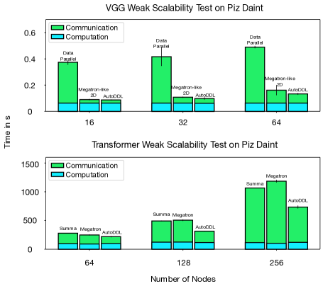
Figure 9: Weak scalability test on the Piz Daint Supercomputer, which has one GPU per node. As the number of nodes increases, we increase the batch size for the VGG model and the number of layers for the Transformer model. A hand-tuned Megatron-like 2d parallel algorithm is applied to VGG’s dense layers. Due to Out-of-Memory, data parallelism can’t be applied to the Transformer models and is hence not included. The error bars show 99% confidence around the mean.

5.2.2 VGG Results

The upper part of figure 9 shows the experiment results for the VGG13 model on the Piz Daint Supercomputer with 16, 32, and 64 nodes. The batch sizes are set to be eight times the number of nodes. The traditional data parallelism is about 4x slower than our AutoDDL-selected strategy throughout the experiments. The 2d distribution for the Megatron-like algorithm is hand-tuned with the best performance. Nevertheless, the AutoDDL-selected strategy performs consistently better than the best hand-tuned Megatron. The performance gap increases with the number of nodes and batch sizes. With 16, 32, and 64 nodes, AutoDDL saves 10%, 18%, and 29% communication time. This result translates to 3%, 8.8%, and 17.7% end-to-end performance benefits compared to the second-best.

5.2.3 Transformer Results

The lower part of figure 9 shows the performance results for Transformer model on the Piz Daint supercomputer. The batch size is fixed to be 1,024 sequences, and each has a length of 1,024 tokens. The number of attention heads is 64 for every layer, and the size of the head dimension is 128. The size of the model dimension is 8,192 throughout the network. We run the model on 64, 128, and 256 nodes with 8, 20, and 44 layers. The number of layers does not increase proportionally with the number of nodes because the input embedding and output logits consume a notable portion of resources and do not change with the number of layers. We set the number of layers so that the compute part is approximately the same on each GPU. These numbers translate to 6.8 billion, 16.5 billion, and 35.8 billion parameters for the models.

We hand-optimized the best 2d node mesh for Summa and Megatron. Data parallelism is impossible since the models cannot fit into a single GPU memory. Megatron performs better than Summa with 64 nodes, but Summa catches up after 128. We attribute it to the fact that Summa can alleviate the memory issues better: If the model gets large and the number of nodes increases, the trade-off between memory and communication becomes prominent. Under these circumstances, Summa can outperform Megatron. However, our AutoDDL-selected strategy performs the best in all cases: For experiments with 64, 128, and 256 GPUs, AutoDDL reduces communication by 23.9%, 46.4%, and 35.3% compared to the second-best baseline. The end-to-end runtime is reduced by 12%, 36.1%, and 31.1%.

5.3 Multi-Node Multi-GPU Results

5.3.1 System Configurations

The experiments are conducted on two DGX A100 servers, and each has 16 NVIDIA A100 with 40 GB GPU memory. The 16 GPUs within the same node are connected via NvLink with 600GB/s peak bandwidth per GPU. The two servers are located in the same compute zone on Google Cloud with 100 Gb/s peak bandwidth. The neural networks are trained in mixed precision since A100 GPU has tensor cores that can deliver 10x more peak performance than full-precision. NCCL is used for communication as default. Moreover, AutoDDL built a communication model for Google Could and selected good parallel strategies for different models, as described in Sections 3 and 4. The AutoDDL strategies are compared against baselines in the following sections.

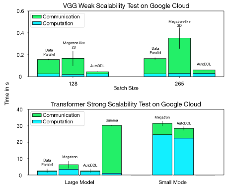
Figure 10: Experiments on the Google Cloud with multiple GPUs per node. We increase the batch size with the number of GPUs per node for the VGG model. For the Transformer model, we increase the model size and fix the number of GPUs for cost reasons. Data parallelism can’t be applied to the large Transformer model due to OOM. Summa parallelism for the large Transformer model is about ten times slower than the best baseline, which is not shown in the figure for clarity. The error bars show 99% confidence around the mean.

5.3.2 VGG Results

Figure 10 shows the results of VGG13 experiments on the Google Cloud Platform. The batch sizes are 128 and 256 on two compute nodes with 4 GPUs and 8 GPUs per node. The Megatron-like algorithm performs the worst and is unstable for both settings. AutoDDL outperforms the other baselines significantly: The communication is reduced by 84.7% and 77.7% respectively, which leads to a reduction of the overall runtime by 71.5% and 63.5%. We have carefully looked into the selected parallel strategy and found that it achieved this significant improvement by 1) avoiding the expensive communication of the model weights gradients and 2) putting a large portion of communication on the fast NvLink. If a 2d algorithm like Megatron were to completely avoid the expensive model weight communication, i.e., with only 1d model parallelism, then no communication can happen over NvLink.

5.3.3 Transformer Results

Figure 10 depicts the strong-scaling performance data for the transformer model on Google Cloud. Due to cost reasons, the system configuration is unchanged and includes two compute nodes, each attached with 16 GPUs. We tested two models for strong scalability: The small model has 24 layers with model dimension 1,024, and the attention operation has 16 attention heads of dimension 64. The large model has 28 layers with model dimension 4,096. The number of the head is 32, each of dimension 128. The batch size is 2 million tokens for both settings: 2,048 sequences with 1,024 tokens per sequence. The small model has 0.35 billion parameters, and the big one has 5.8 billion. The small model can fit into a single GPU memory, and data parallelism is the best parallel strategy compared with other baselines. In this case, AutoDDL selects data parallelism as the best strategy. For the large model that we can’t apply data parallelism, AutoDDL selects a strategy that has 21.6% less communication, resulting in 10% less runtime than Megatron. AutoDDL can still beat Megatron when data parallelism is unavailable due to OOM.

5.4 Combined with Pipeline Parallelism

   Model Scheme Nodes Opt. Stages Time    Transformer Megatron 64 1 533s    Wide AutoDDL 335s Megatron 128 503s AutoDDL 315s    Transformer Megatron 64 2 710s    Deep AutoDDL 443s Megatron 128 807s AutoDDL 508s

Table 3: Performance results for Megatron and AutoDDL with pipeline parallelism enabled. The sizes of the wide and deep models are described in Section 5.4. The batch size increases linearly with the number of nodes. Opt. Stage denotes the optimal pipeline stages.

Pipeline parallelism is an orthogonal technique for DNNs training with deep repeated structures. Non-regular models, like many CNNs, are not best-suited for pipeline parallelism. Megatron [31] combines data-, operator- and pipeline parallelisms to train more regular Transformer networks with repeated structures. In this section, we show that AutoDDL provides performance benefits against hand-tuned Megatron even when pipeline parallelism is enabled.

We have tested two Transformer models with different sizes: The deeper model has 36 layers, model dimension 4,096, and 32 attention heads, each of size 128. The wider model has 20 layers with model dimension 8,192, 64 attention heads of size 128. Notably, the wider model is consistent with our previous experiments on the Piz Daint Supercomputer. We have tested the models with different pipeline stages and report the best one. The micro-batch for each pipeline stage is the smallest to maximize pipeline utilization. The operator- and data- parallelisms are hand-tuned to be optimal for Megatron and automatically generated for AutoDDL.

Pipeline parallelism splits a batch into micro-batch. Different micro-batches work on different pipeline stages in parallel. We have not included Summa since 1) Summa is inherently expensive when coupled with pipeline parallelism. Summa splits the model weights in 2d without any replication. Each pipeline micro-batch must communicate the whole model, whereas AutoDDL and Megatron only communicate the model gradients when a batch is complete. 2) Unlike the other two methods, one would have to hand-tune the number of micro-batches for each number of pipeline stages: smaller micro-batch size implies better pipeline utilization but more model weights communications. In addition, the 2d mesh of nodes needs to be tuned. Finding the best pipelined Summa requires much more computing power and engineering efforts.

Table 3 shows the experiment results for the wide and deep models on 64 and 128 nodes of the Piz Daint Supercomputer. The batch sizes are 512 and 1,024 sequences, each sequence with 1,024 tokens. Even with pipeline parallelism, the communication bottleneck remains in data- and model parallelism: Pipeline parallelism introduces only one point-to-point intermediate result communication between pipeline stages. On the contrary, model parallelism communications the same intermediate result using more expensive collectives for each layer. Our AutoDDL searched strategy leverages the communication bottleneck and outperforms Megatron with pipeline parallelism in all experiments in Table 3.

6 Conclusions

AutoDDL enables automatic distributed deep learning with easy code implementation and an asymptotically optimal guarantee. Based on the abstraction of SBP, we defined a space of parallel DNN execution schemes that can be conveniently implemented in OneFlow. We have shown that the search space contains asymptotically communication-optimal strategies. Furthermore, we have built a performance model and established efficient heuristic search algorithms for quickly finding a communication-reducing distributed execution plan in the search space.

We have tested AutoDDL for VGG and GPT models on the Piz Daint Supercomputer with multi-nodes-single-GPU and the Google Cloud Platform with multi-nodes-multi-GPUs. We have experimentally compared AutoDDL’s performance with data parallelism, Summa distribution matrix multiplication algorithm, and Megatron parallelism. AutoDDL outperforms the baselines in all experiments. AutoDDL can be easily combined with orthogonal methods like pipeline parallelism and still outperforms Megatron when pipeline parallelism is enabled.

The key takeaways are as follows:

(1) Near-optimal strategy search in a per-layer granularity is the key to performance improvement. Each neural network training process has varying batch sizes and many layers, and these layers may have different structures and sizes. Hence, each layer of every training process might suit a distinct strategy. The last three dense layers of VGG13 shown in Figure 7 are examples of different strategies selected for the three layers adapted to each layer’s sizes and dimensions.

(2) A more extensive search space with asymptotically optimal execution plans can provide performance benefits. Even though asymptotic does not always reflect actual runtime, a larger search space can often contain better parallel execution schemes. AutoDLL extends its search space with a new Partial-Sum state, whereas previous automatic frameworks like Alpa and Flexflow build upon the GShard abstraction. Experiments show that AutoDDL provides performance benefits against expert-designed Megatron using Partial-Sum in its selected strategies, whereas previous works can not.

(3) An accurate performance model and heuristic search algorithms enable fast search. In our experiments, the search process can finish in minutes using a personal Laptop. A faster search with fewer overheads can be even more desirable if one wants to run more complex models or extend the search space in future systems.

Overall, AutoDDL realizes automatic distributed deep learning and asymptotically optimal communication simultaneously, which has not been done in previous work.

References

- [1] Abadi, M., Barham, P., Chen, J., Chen, Z., Davis, A., Dean, J., Devin, M., Ghemawat, S., Irving, G., Isard, M., et al. TensorFlow: A system for Large-Scale machine learning. In 12th USENIX symposium on operating systems design and implementation (OSDI 16) (2016), pp. 265–283.
- [2] Andrieu, C., de Freitas, N., Doucet, A., and Jordan, M. I. An introduction to mcmc for machine learning. Machine Learning 50 (2004), 5–43.
- [3] Ben-Nun, T., and Hoefler, T. Demystifying Parallel and Distributed Deep Learning: An In-Depth Concurrency Analysis. ACM Comput. Surv. 52, 4 (Aug. 2019), 65:1–65:43.
- [4] Bian, Z., Xu, Q., Wang, B., and You, Y. Maximizing parallelism in distributed training for huge neural networks. arXiv preprint arXiv:2105.14450 (2021).
- [5] Brown, T., Mann, B., Ryder, N., Subbiah, M., Kaplan, J. D., Dhariwal, P., Neelakantan, A., Shyam, P., Sastry, G., Askell, A., et al. Language models are few-shot learners. Advances in neural information processing systems 33 (2020), 1877–1901.
- [6] Chen, A., Demmel, J., Dinh, G., Haberle, M., and Holtz, O. Communication bounds for convolutional neural networks. In Proceedings of the Platform for Advanced Scientific Computing Conference (New York, NY, USA, 2022), PASC ’22, Association for Computing Machinery.
- [7] Chen, T., Xu, B., Zhang, C., and Guestrin, C. Training deep nets with sublinear memory cost. ArXiv abs/1604.06174 (2016).
- [8] Demmel, J., Eliahu, D., Fox, A., Kamil, S., Lipshitz, B., Schwartz, O., and Spillinger, O. Communication-optimal parallel recursive rectangular matrix multiplication. International Symposium on Parallel and Distributed Processing (2013).
- [9] Dryden, N., Maruyama, N., Benson, T., Moon, T., Snir, M., and Essen, B. V. Improving strong-scaling of cnn training by exploiting finer-grained parallelism. International Parallel and Distributed Processing Symposium (2019).
- [10] Dryden, N., Maruyama, N., Moon, T., Benson, T., Snir, M., and Essen, B. C. V. Channel and filter parallelism for large-scale cnn training. Proceedings of the International Conference for High Performance Computing, Networking, Storage and Analysis (2019).
- [11] Du, N., Huang, Y., Dai, A. M., Tong, S., Lepikhin, D., Xu, Y., Krikun, M., Zhou, Y., Yu, A. W., Firat, O., et al. Glam: Efficient scaling of language models with mixture-of-experts. arXiv preprint arXiv:2112.06905 (2021).
- [12] Essen, B. V., Kim, H., Pearce, R., and Chen, K. B. B. Lbann: Livermore big artificial neural network hpc toolkit. Proceedings of the Workshop on Machine Learning in High-Performance Computing Environments (2015).
- [13] Fan, S., Rong, Y., Meng, C., Cao, Z., Wang, S., Zheng, Z., Wu, C., Long, G., Yang, J., Xia, L., Diao, L., Liu, X., and Lin, W. Dapple: a pipelined data parallel approach for training large models. Proceedings of the 26th ACM SIGPLAN Symposium on Principles and Practice of Parallel Programming (2021).
- [14] Farsa, D. Z., and Rahnamayan, S. Discrete coordinate descent (dcd). 2020 IEEE International Conference on Systems, Man, and Cybernetics (SMC) (2020), 184–190.
- [15] Hastings, W. K. Monte carlo sampling methods using markov chains and their applications. Biometrika 57 (1970), 97–109.
- [16] Hoefler, T., and Belli, R. Scientific benchmarking of parallel computing systems: twelve ways to tell the masses when reporting performance results. SC15: International Conference for High Performance Computing, Networking, Storage and Analysis (2015), 1–12.
- [17] Hoefler, T., Bonato, T., Sensi, D. D., Girolamo, S. D., Li, S., Heddes, M., Belk, J., Goel, D., and Miguel Castro, S. S. HammingMesh: A Network Topology for Large-Scale Deep Learning. In Proceedings of the International Conference for High Performance Computing, Networking, Storage and Analysis (SC’22) (Nov. 2022).
- [18] Huang, Y., Cheng, Y., Bapna, A., Firat, O., Chen, M. X., Chen, D., Lee, H., Ngiam, J., Le, Q. V., Wu, Y., and Chen, Z. Gpipe: Efficient training of giant neural networks using pipeline parallelism. Advances in Neural Information Processing Systems (2018).
- [19] Jia, Z., Zaharia, M., and Aiken, A. Beyond data and model parallelism for deep neural networks. Proceedings of the 2nd Conference on Machine Learning and Systems (2018).
- [20] Kahira, A. N., Nguyen, T. T., Bautista-Gomez, L. A., Takano, R., Badia, R. M., and Wahib, M. An oracle for guiding large-scale model/hybrid parallel training of convolutional neural networks. Proceedings of the 30th International Symposium on High-Performance Parallel and Distributed Computing (2021).
- [21] Kaplan, J., McCandlish, S., Henighan, T. J., Brown, T. B., Chess, B., Child, R., Gray, S., Radford, A., Wu, J., and Amodei, D. Scaling laws for neural language models. ArXiv abs/2001.08361 (2020).
- [22] Krizhevsky, A. One weird trick for parallelizing convolutional neural networks. ArXiv abs/1404.5997 (2014).
- [23] Kwasniewski, G., Kabić, M., Besta, M., VandeVondele, J., Solcà, R., and Hoefler, T. Red-blue pebbling revisited: Near optimal parallel matrix-matrix multiplication. In Proceedings of the International Conference for High Performance Computing, Networking, Storage and Analysis (2019).
- [24] Lepikhin, D., Lee, H., Xu, Y., Chen, D., Firat, O., Huang, Y., Krikun, M., Shazeer, N. M., and Chen, Z. Gshard: Scaling giant models with conditional computation and automatic sharding. ICLR ’21 (2020).
- [25] Li, M., Andersen, D. G., Park, J. W., Smola, A., Ahmed, A., Josifovski, V., Long, J., Shekita, E. J., and Su, B.-Y. Scaling distributed machine learning with the parameter server. In BigDataScience ’14 (2014).
- [26] Li, S., and Hoefler, T. Chimera: Efficiently training large-scale neural networks with bidirectional pipelines. In Proceedings of the International Conference for High Performance Computing, Networking, Storage and Analysis (New York, NY, USA, 2021), SC ’21, Association for Computing Machinery.
- [27] Li, Z., Zhuang, S., Guo, S., Zhuo, D., Zhang, H., Song, D. X., and Stoica, I. Terapipe: Token-level pipeline parallelism for training large-scale language models. ArXiv abs/2102.07988 (2021).
- [28] Narayanan, D., Harlap, A., Phanishayee, A., Seshadri, V., Devanur, N., Granger, G., Gibbons, P., and Zaharia, M. Pipedream: Generalized pipeline parallelism for dnn training. The 27th ACM Symposium on Operating Systems Principles (2019).
- [29] Narayanan, D., Phanishayee, A., Shi, K., Chen, X., and Zaharia, M. A. Memory-efficient pipeline-parallel dnn training. In ICML (2021).
- [30] Narayanan, D., Shoeybi, M., Casper, J., LeGresley, P., Patwary, M., Korthikanti, V., Vainbrand, D., Kashinkunti, P., Bernauer, J., Catanzaro, B., et al. Efficient large-scale language model training on gpu clusters using megatron-lm. In Proceedings of the International Conference for High Performance Computing, Networking, Storage and Analysis (2021), pp. 1–15.
- [31] Narayanan, D., Shoeybi, M., Casper, J., LeGresley, P., Patwary, M., Korthikanti, V., Vainbrand, D., Kashinkunti, P., Bernauer, J., Catanzaro, B., Phanishayee, A., and Zaharia, M. Efficient large-scale language model training on GPU clusters. SC (2021).
- [32] Nguyen, T. T., Wahib, M., and Takano, R. Efficient mpi-allreduce for large-scale deep learning on gpu-clusters. Concurrency and Computation: Practice and Experience 33 (2019).
- [33] Paszke, A., Gross, S., Massa, F., Lerer, A., Bradbury, J., Chanan, G., Killeen, T., Lin, Z., Gimelshein, N., Antiga, L., et al. Pytorch: An imperative style, high-performance deep learning library. Advances in neural information processing systems 32 (2019).
- [34] Patarasuk, P., and Yuan, X. Bandwidth optimal all-reduce algorithms for clusters of workstations. J. Parallel Distributed Comput. 69 (2009), 117–124.
- [35] Schatz, M. D., Geijn, R. A., and Poulson, J. Parallel matrix multiplication: A systematic journey. SIAM J. Sci. Comput. 38 (2016).
- [36] Scquizzato, M., and Silvestri, F. Communication lower bounds for distributed-memory computations. Journal of Parallel and Distributed Computing (2014).
- [37] Sergeev, A., and Balso, M. D. Horovod: fast and easy distributed deep learning in tensorflow. ArXiv abs/1802.05799 (2018).
- [38] Solomonik, E., and Demmel, J. Communication-optimal parallel 2.5 d matrix multiplication and lu factorization algorithms. In European Conference on Parallel Processing (2011), Springer, pp. 90–109.
- [39] Wright, S. J. Coordinate descent algorithms. Mathematical Programming 151 (2015), 3–34.
- [40] Wu, Y., Schuster, M., Chen, Z., Le, Q. V., Norouzi, M., Macherey, W., Krikun, M., Cao, Y., Gao, Q., Macherey, K., Klingner, J., Shah, A., Johnson, M., Liu, X., Kaiser, L., Gouws, S., Kato, Y., Kudo, T., Kazawa, H., Stevens, K., Kurian, G., Patil, N., Wang, W., Young, C., Smith, J. R., Riesa, J., Rudnick, A., Vinyals, O., Corrado, G. S., Hughes, M., and Dean, J. Google’s neural machine translation system: Bridging the gap between human and machine translation. ArXiv abs/1609.08144 (2016).
- [41] Xu, Q., Li, S., Gong, C., and You, Y. An efficient 2d method for training super-large deep learning models. arXiv preprint arXiv:2104.05343 (2021).
- [42] Yang, B., Zhang, J., Li, J., Ré, C., Aberger, C. R., and Sa, C. D. Pipemare: Asynchronous pipeline parallel DNN training. CoRR abs/1910.05124 (2019).
- [43] Yuan, J., Li, X., Cheng, C., Liu, J., Guo, R., Cai, S., Yao, C., Yang, F., Yi, X., Wu, C., Zhang, H., and Zhao, J. Oneflow: Redesign the distributed deep learning framework from scratch. CoRR abs/2110.15032 (2021).
- [44] Zheng, L., Li, Z., Zhang, H., Zhuang, Y., Chen, Z., Huang, Y., Wang, Y., Xu, Y., Zhuo, D., Gonzalez, J., and Stoica, I. Alpa: Automating inter- and intra-operator parallelism for distributed deep learning. ArXiv abs/2201.12023 (2022).