KAOSS: turbulent, but disc-like kinematics in dust-obscured star-forming galaxies at $z$ $\sim$ 1.3–2.6

Abstract

We present spatially resolved kinematics of 31 ALMA-identified dust-obscured star-forming galaxies (DSFGs) at $z$ $\sim$ 1.3–2.6, as traced by H$\alpha$ emission using VLT/KMOS near-infrared integral field spectroscopy from our on-going Large Programme “KMOS-ALMA Observations of Submillimetre Sources” (KAOSS). We derive H$\alpha$ rotation curves and velocity dispersion profiles for the DSFGs. Of the 31 sources with bright, spatially extended H$\alpha$ emission, 25 display rotation curves that are well fit by a Freeman disc model, enabling us to measure a median inclination-corrected velocity at 2.2 $R_{\rm d}$ of $v_{\rm rot}$ $=$ 190 $\pm$ 30 km s^-1 and a median intrinsic velocity dispersion of $\sigma_{0}$ $=$ 87 $\pm$ 6 km s^-1 for these disc-like sources. By comparison with less actively star-forming galaxies, KAOSS DSFGs are both faster rotating and more turbulent, but have similar $v_{\rm rot}/\sigma_{0}$ ratios, median 2.4 $\pm$ 0.5. We suggest that $v_{\rm rot}/\sigma_{0}$ alone is insufficient to describe the kinematics of DSFGs, which are not kinematically “cold” discs, and that the individual components $v_{\rm rot}$ and $\sigma_{0}$ indicate that they are in fact turbulent, but rotationally supported systems in $\sim$ 50 per cent of cases. This turbulence may be driven by star formation or mergers/interactions. We estimate the normalisation of the stellar Tully-Fisher relation (sTFR) for the disc-like DSFGs and compare it with local studies, finding no evolution at fixed slope between $z$ $\sim$ 2 and $z$ $\sim$ 0. Finally, we use kinematic estimates of DSFG halo masses to investigate the stellar-to-halo mass relation, finding our sources to be consistent with shock heating and strong feedback which likely drives the declining stellar content in the most massive halos.

1 Introduction

Dust-obscured star-forming galaxies (DSFGs) at the peak of cosmic star formation ($z$ $\sim$ 2) are massive and gas rich, with star-formation rates (SFRs) that are significantly higher than typical systems at this epoch (also see e.g. Tacconi et al., 2006; Magnelli et al., 2012; Bothwell et al., 2013; Swinbank et al., 2014; Miettinen et al., 2017; Dudzevičiūtė et al., 2020; Birkin et al., 2021; Shim et al., 2022). However, their kinematics are poorly understood due to a lack of spatially resolved observations. Are they predominantly turbulent merger-driven (e.g. Narayanan et al., 2009, 2010; Lagos et al., 2020) systems, like the similarly infrared-bright local Ultra-Luminous Infrared Galaxy (ULIRG) population (e.g. Bellocchi et al., 2016)? Or do they more closely resemble regular discs that are smoothly accreting gas from the intergalactic medium (IGM; Kereš et al., 2005; Dekel & Birnboim, 2006; Narayanan et al., 2015; Tacconi et al., 2020)?

One of the most promising routes to test these competing theories is through integral field spectroscopy (IFS) in the rest-frame optical, which enables two-dimensional (2-D) mapping of the spatially resolved kinematics via nebular emission lines such as H$\alpha$ (e.g. Cresci et al., 2009; Förster Schreiber et al., 2009; Alaghband-Zadeh et al., 2012; Wisnioski et al., 2015, 2019; Tiley et al., 2021). These maps can then be used to measure the rotational velocity $v_{\rm rot}$ and intrinsic velocity dispersion $\sigma_{0}$ (e.g. Förster Schreiber et al., 2009; Wisnioski et al., 2015, 2019; Johnson et al., 2018). In the local Universe there are several comprehensive studies of galaxy kinematics, with surveys such as the Calar Alto Legacy Integral Field Area (CALIFA; Sánchez et al., 2012), the Sydney–Australian–Astronomical Observatory Multi-Object Integral-field Spectrograph (SAMI; Croom et al., 2012) and Mapping Nearby Galaxies at Apache Point Observatory (MANGA; Bundy et al., 2015) providing IFU observations of the gas and stellar motions in thousands of $z$ $\sim$ 0 galaxies spanning a range of stellar masses.

At $z$ $\sim$ 2, the rest frame-optical nebular emission lines such as H$\alpha$ and [Oiii] are redshifted into the near-infrared (NIR) and into the coverage of instruments such as the $K$-band Multi-Object Spectrograph (KMOS; Sharples et al., 2013). However, dynamical analyses with KMOS at this epoch are challenging because of the seeing-limited spatial resolution – KMOS achieves a resolution of $\sim$ 0.6^′′ (FWHM), which corresponds to a physical size of $\sim$ 5 kpc at $z=$ 2 (although finer spatial scales can be sampled if the sources exhibit velocity gradients). Additionally the $H$ band, which covers the redshifted H$\alpha$ emission from galaxies at $z$ $\sim$ 1.2–1.8, suffers from strong sky contamination (Soto et al., 2016; Tiley et al., 2021) that can be challenging to robustly model and remove.

As a result, the tools used to study kinematics at high redshifts are different to those used at low redshifts. Instead of studying detailed scaling relations, measurements of the ratio of rotational velocity to intrinsic velocity dispersion $v_{\rm rot}/\sigma_{0}$ have been used (Weiner et al., 2006; Newman et al., 2013; Wisnioski et al., 2015) in an attempt to quantify the kinematics. For example, galaxies with $v_{\rm rot}/\sigma_{0}>$ 1.5 have been considered to be rotationally supported (e.g. Stott et al., 2016; Tiley et al., 2021), whereas galaxies with $v_{\rm rot}/\sigma_{0}<$ 1.5 are believed to be dominated by turbulent motions that may indicate an on-going or recent merger (e.g. Alaghband-Zadeh et al., 2012).

Progress in NIR integral field spectrograph technology has allowed IFU studies of increasing numbers of high-redshift sources in recent years, and as in the local Universe there are now several large surveys of spatially resolved kinematics with KMOS and SINFONI including the Spectroscopic Imaging survey in the near-infrared with SINFONI (SINS/zC-SINF; Förster Schreiber et al., 2009; Mancini et al., 2011), the KMOS Redshift One Spectroscopic Survey (KROSS; Stott et al., 2016), the KMOS^3D survey (Wisnioski et al., 2015, 2019), the KMOS Deep Survey (KDS; Turner et al., 2017) and the KMOS Galaxy Evolution Survey (KGES; Tiley et al., 2021). These surveys cover the epoch when the star-formation rate density (SFRD) is at its peak, $z$ $\sim$ 1–2, and when a significant proportion of the stellar mass we see in the local Universe was assembled. These surveys have revealed that high-redshift star-forming galaxies appear dynamically “hot” when compared to local galaxies (e.g Förster Schreiber et al., 2009; Wisnioski et al., 2015, 2019; Stott et al., 2016; Johnson et al., 2018).

These surveys also enable another probe of galaxy evolution: the Tully-Fisher relation (TFR; Tully & Fisher, 1977) – the relationship between galaxy luminosity and rotational velocity – which can trace the evolution of star-forming galaxies between $z$ $\sim$ 2 and $z$ $\sim$ 0. The TFR has been well studied at $z$ $\sim$ 0 (Tully & Pierce, 2000; Lagattuta et al., 2013). Surveys at $z$ $\sim$ 2 find much greater scatter in the relation potentially due to the increased turbulence in the star-forming galaxy population (e.g. Gnerucci et al., 2011), and these studies have made conflicting claims about the evolution of the TFR. Some find no evolution at all (e.g. Conselice et al., 2005; Kassin et al., 2007; Übler et al., 2017; Tiley et al., 2019), suggesting a close link between the build up of stellar mass and dark matter in $z$ $\sim$ 2 SFGs, others find evidence for an evolution of the zero point with redshift (e.g. Cresci et al., 2009; Swinbank et al., 2012; Übler et al., 2017) which would imply differing growth rates of the two matter components with cosmic time.

In contrast to these studies of typical star-forming galaxies, spatially resolved kinematic studies of the more massive and active DSFGs however, have been much more limited in scope. Among the few published studies are Swinbank et al. (2006), who found four of their sample of six DSFGs to contain multiple components and Alaghband-Zadeh et al. (2012), who observed nine DSFGs at $z$ $\sim$ 2.0–2.7 with SINFONI and the Gemini-North/Near-Infrared Integral Field Spectrograph (NIFS), measuring an average H$\alpha$ velocity dispersion of $\sigma$ $=$ 220 $\pm$ 80 km s^-1 indicating large amounts of turbulence in these sources. Additionally, they found that six of the nine sources showed multiple kinematically distinct components, and they classified all nine sources as mergers based on kinemetry of the velocity and velocity dispersion maps. Similarly, Menéndez-Delmestre et al. (2013) observed three DSFGs with the OH-Suppressing Infrared Imaging Spectrograph (OSIRIS) on the Keck telescope, finding the systems to contain multiple clumps that they suggested to be in the process of merging, and thus driving high SFRs. More recently, Olivares et al. (2016) observed eight DSFGs at $z$ $\sim$ 1.3–2.5 with SINFONI, finding irregular/clumpy velocity and velocity dispersion fields, which they also interpreted as evidence for galaxy-galaxy interactions and/or mergers.

Studying the kinematics of high-redshift DSFGs is one of the main goals of our KMOS Large Programme “KMOS+ALMA Observations of Submillimetre Sources” (KAOSS). KAOSS targets $\sim$ 400 DSFGs with KMOS in the $HK$ filter (approximately half have been observed thus far), which covers the H$\alpha$ and/or [Oiii] emission lines at $z$ $\sim$ 1–3, and in this paper we will utilise KAOSS to map the H$\alpha$ emission in the brightest, extended sources, from which we will extract velocity fields and rotation curves. Our goal is to significantly increase the sample of DSFGs with spatially resolved measurements of rotational velocities and intrinsic velocity dispersions, along with $v_{\rm rot}/\sigma_{0}$, the latter of which has been claimed to be a key diagnostic of the level of rotational support in galaxies (e.g. Wisnioski et al., 2019).

In this paper we present the properties of a subset of 31 KAOSS sources in the COSMOS, UDS and GOODS-S fields, with sufficiently bright and extended H$\alpha$ detections to yield robust 2-D kinematic information. The outline of this paper is as follows: in §2 and §3 we describe the sample studied and the observations carried out, along with our data reduction and analysis methods, before discussing the measurements made. In §4 we discuss the results and their implications. In §5 we summarise our findings. Throughout this paper we adopt a flat $\Lambda$-CDM cosmology defined by ($\Omega_{\mathrm{m}}$, $\Omega_{\Lambda}$, H₀) $=$ (0.3, 0.7, 70 km s^-1 Mpc^-1).

2 Sample selection and observations

2.1 Sample

We exploit KMOS data from the KAOSS Large Programme (Programme ID: 1103.A-0182). These are 13.5-ks exposure observations of DSFGs in the $HK$ grating ($\sim$ 1.4–2.4 $\mu$m) with KMOS on the Very Large Telescope (VLT), designed to obtain NIR redshifts and spatially resolved emission-line detections. The KAOSS targets were selected from four ALMA surveys:

• AS2UDS (Stach et al., 2019): ALMA 870 $\mu$m follow up of 712 SCUBA-2 sources from a deep 1 sq. degree SCUBA-2 map of the UKIDSS Ultra Deep Survey (UDS) field (Geach et al., 2017),

• AS2COSMOS (Simpson et al., 2020): ALMA 870 $\mu$m pilot follow up of the 160 brightest SCUBA-2 sources from a deep 2 sq. degree SCUBA-2 map of the Cosmic Evolution Survey (COSMOS) field (Simpson et al., 2019) (when completed this survey will have observed 1200 sources),

• ALESS and BASIC (Hodge et al., 2013; Cowie et al., 2018): ALMA follow up of 179 LABOCA or SCUBA-2 sources in GOODS-S/ECDFS,

• A3COSMOS (Liu et al., 2019): pipeline exploiting the ALMA archive to locate submillimetre-detected galaxies in the COSMOS field.

When selecting targets for the KMOS IFUs we prioritise sources that are brighter in the $K$ band, as they are more likely to yield emission-line detections in our 13.5 ks exposures (see §2.3), and also more likely to yield resolved kinematics.

For this paper, we select KAOSS sources with H$\alpha$ detections that are bright enough to search for resolved velocity structure from the H$\alpha$ emission line. All sources with line detections from KAOSS are fit on a spaxel-by-spaxel basis, as we will describe in §3.3. We consider a source to be kinematically “resolved” if the fitting successfully reproduces a velocity map (according to the S/N criterion described in §3.3) with more than 20 adjacent (0.1^′′ $\times$ 0.1^′′) pixels. This results in a sample of 31 H$\alpha$ sources with $f_{{\rm H}\alpha}>$ 1.7 $\times$ 10^-20 W m^-2 at $z$ $=$ 1.3–2.6, all of which have a signal-to-noise ratio of S/N $>$ 7 for the H$\alpha$ emission line in the integrated spectrum.

2.2 Physical properties and comparison with other survey samples

Before discussing the resolved kinematics, we place our sample in context with samples from other galaxy surveys. In Fig. 1 we show the 870-$\mu$m fluxes of the KAOSS sample versus their $K$-band magnitudes. As a comparison sample we show in Fig.1 the 707 DSFGs from the ALMA-SCUBA-2 Ultra Deep Survey (AS2UDS; Stach et al., 2019; Dudzevičiūtė et al., 2020), which is the largest sample of 870 $\mu$m-selected DSFGs and therefore provides a good indicator of the properties of the general 870 $\mu$m-selected population. Our KAOSS sample spans the range of 870-$\mu$m fluxes in AS2UDS, $S_{870}$ $\sim$ 0.5–14 mJy, although the resolved subset only samples sources with $K\lesssim$ 22.9.

We primarily aim to compare with less actively star-forming galaxies, and so we also show in Fig. 1 $z$ $\sim$ 1.5 $K$-band-selected star-forming galaxies from the KMOS Galaxy Evolution Survey (KGES; Tiley et al., 2021). 870-$\mu$m fluxes are not available for these sources, but they do have magphys-derived dust mass estimates, which we convert to $S_{870}$ estimates using the $M_{\rm dust}$–$S_{870}$ relation derived by Dudzevičiūtė et al. (2020). These are therefore approximate values, but they highlight the region of the parameter space probed by the KGES sample. In general, KGES galaxies have lower submillimetre fluxes than KAOSS, but comparable rest-frame optical fluxes.

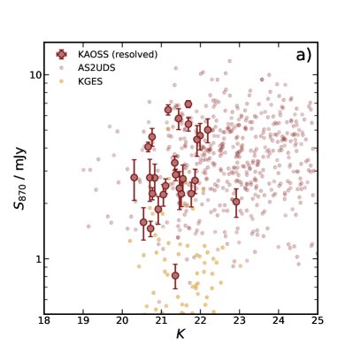
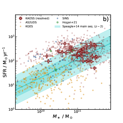
Figure 1: a) $K$-band magnitude versus 870-$\mu$m flux density ($S_{870}$) for the KAOSS resolved sample compared with the 707 AS2UDS DSFGs (Dudzevičiūtė et al., 2020) and $z$ $\sim$ 1.5 star-forming galaxies from KGES (Tiley et al., 2021). The KAOSS resolved sample is generally representative of the range of 870-$\mu$m flux densities in the DSFG population, but biased towards near-infrared-brighter sources. For the KGES sample we indicate the region containing the $K$-band magnitudes of the sample and the expected 870-$\mu$m flux densities estimated from SED-derived dust masses. The KAOSS sample is complemented by KGES in that the latter extends the range in SFR by an order of magnitude. b) Star-formation rate versus $M_{\ast}$ for the same samples, now also including six $z$ $\sim$ 2.5 ULIRGs from Hogan et al. (2021). KAOSS probes sources that are approximately an order of magnitude more massive than KGES, and overlaps with the parameter range of the Herschel-selected ULIRGs in Hogan et al. (2021). Also shown here are $z$ $\sim$ 1.3–2.6 UV/optically selected galaxies from the SINS survey (Förster Schreiber et al., 2009), which has some overlap with KAOSS, but also probes lower-mass and lower-SFR systems.

In Fig. 1 we also show star-formation rates (SFRs) versus stellar masses ($M_{\ast}$) taken from pre-existing magphys spectral energy distribution (SED) fits for our sample. For details on the SED fitting for these sources we direct the reader to da Cunha et al. (2015), Dudzevičiūtė et al. (2020) and Ikarashi et al. (in prep.). These fits are performed using the photo-$z$ extension of the code, and therefore the redshifts are probabilistic in the modelling at this point. In §3.4 we will repeat the fits for sources with spectroscopic redshifts from KAOSS. Open circles represent sources that are detected, but unresolved, and therefore not analysed in this paper. We also show the star-forming main sequence at $z$ $=$ 2 according to the prescription of Speagle et al. (2014). The 31 resolved KAOSS sources have median stellar masses and star-formation rates of $M_{\ast}$ $=$ (1.3 $\pm$ 0.2) $\times$ 10¹¹ M_⊙ and SFR $=$ 220 $\pm$ 30 M_⊙yr^-1. To compare this with other DSFGs, we select the 283 AS2UDS sources lying in the range $z=$ 1.3–2.6, encompassing all the resolved KAOSS sources. These have median stellar masses and SFRs of $M_{\ast}$ $=$ (1.44 $\pm$ 0.01) $\times$ 10¹¹ M_⊙ and SFR $=$ 173 $\pm$ 6 M_⊙yr^-1, hence in this analysis we are probing DSFGs that are generally representative of the stellar masses in the 870 $\mu$m-selected population, but slightly more active in terms of star-formation rate.

Fig. 1 confirms that the KGES sample probes much less massive and less actively star-forming sources, with median stellar masses and SFRs of $M_{\ast}$ $=$ (1.3 $\pm$ 0.1) $\times$ 10¹⁰ M_⊙ and SFR $=$ 16 $\pm$ 1 M_⊙yr^-1, respectively, approximately an order of magnitude lower than the KAOSS resolved sample in both cases. Therefore, by supplementing our results with those from KGES we will be able to study the variation of kinematic properties across a wider range in stellar mass and star-formation rate.

As a further comparison sample of similar galaxies, in Fig. 1 we include data from KMOS observations of six $z$ $\sim$ 2.5 Herschel-selected ULIRGs with kinematical information estimated by Hogan et al. (2021). While these sources are selected based on shorter far-infrared wavelengths than our DSFGs, they are gas-rich star-forming galaxies at comparable redshifts to the most distant sources in our resolved sample, which spans the range $z$ $\sim$ 1.5–2.5. Indeed, the six sources from Hogan et al. (2021) have median stellar masses and SFRs of $M_{\ast}$ $=$ (2.5 $\pm$ 1.5) $\times$ 10¹¹ M_⊙ and SFR $=$ 130 $\pm$ 90 M_⊙ yr^-1, consistent with the KAOSS resolved sample. Where possible we compare our results with both the KGES and Hogan et al. (2021) ULIRG samples throughout our analysis.

2.3 Observing strategy

KMOS (Sharples et al., 2013) is a near-infrared multi-object spectrograph mounted at the Nasmyth focus of Unit Telescope 1 on the VLT. It is comprised of 24 IFUs that patrol a field of 7.2^′ diameter area of the sky, with each IFU covering a 2.8^′′ $\times$ 2.8^′′ field of view sampled by 14 $\times$ 14 spaxels (0.2^′′ per pixel). In our survey fields KMOS pointings typically contain $\sim$ 10 DSFGs, and as KMOS has 24 IFUs available, and given the need for sky offsets, we choose to pair IFUs on our targets and a matched blank sky region where possible. This maximises the on-target time. When observing, the instrument nods back and forth between the target and a sky position in order to assist sky subtraction. By creating sky positions offset relative to the corresponding target position by a similar fixed vector, we can ensure that the target is observed by either the primary or secondary (sky) IFU at all times.

The final reduced frames corresponding to the target in both the primary or secondary IFUs can be combined to increase the signal-to-noise ratio (S/N). This pairing of these IFUs is not always possible given the positioning of targets within the field of view, but we prioritise this approach for sources with $K$ $<$ 22.5 that are most likely to yield spatially resolved kinematics. We also reserve one IFU to be placed on a bright ($H\sim$ 12–15) star, allowing us to monitor the telescope pointing and the point spread function (PSF).

Each observing block (OB) yields 2.7 ks of on-source integration time in around an hour of telescope time. To obtain our desired sensitivity of $\sim$ 1 $\times$ 10^-20 W m^-2 we observe each OB five times, resulting in a total exposure time of 13.5 ks for each pointing. Observations are carried out in the combined $HK$ grating, which covers the wavelength range $\lambda\sim$ 1.4–2.4 $\mu$m at a spectral resolution of $\delta\lambda$/$\lambda$ $\sim$ 2000. This is sufficient to cover the H$\alpha$ emission line for sources at $z$ $\sim$ 1.1–2.7 where the majority of our targets are expected to reside, given their photometric redshifts.

3 Data reduction and analysis

3.1 KMOS data reduction

In this section we provide a brief description of the processes taken to produce fully reduced data cubes from the raw KMOS data, following the approach used by Tiley et al. (2021). Full details will be provided in Birkin et al. (in prep.) and can also be found in Birkin (2022). Calibration of the raw data products proceeds via the European Southern Observatory (ESO) Recipe Execution Tool (esorex; ESO CPL Development Team, 2015), a library of functions that take as an input the raw data and produce reduced 3D cubes.

While the standard esorex pipeline carries out a basic A$-$B sky subtraction, this is often poor in the $HK$ band of KMOS, therefore we employ a more sophisticated technique based on the Zurich Atmospheric Purge (ZAP; Soto et al., 2016) method initially developed for the MUSE instrument, with optimisations made for KMOS observations. The ZAP method is based on principal component analysis (PCA), using filtering and data segmentation to reduce sky emission residuals while preserving flux from the astronomical target. This KMOS-adapted method is encapsulated in the pyspark code (Mendel et al. in prep.).

As previously stated, in every OB we assign at least one IFU to a bright star, one of the primary purposes of which is to centre the data cubes between OBs. Therefore, for each set of AB pairs we obtain a reduced cube of a bright star, and we measure the centroid of the emission in this cube by collapsing it and fitting a 2-D Gaussian profile to the spatial emission. We then shift all observations of that field to a common centre using the measured centroid from the star. We also check for any significant offset in the final cubes between individual observations. This allows us to be confident that we are not losing S/N in our combined cubes, as a result of misalignment. Small perturbations can affect the alignment of the telescope, and while in theory these should be corrected for in the acquisition and data reduction, we check each observing block ($\sim$ 1 hr exposure) for offsets by comparing the measured position of any sources bright enough in their continuum or line emission to be detected. Once the reduced cubes have been produced and aligned, we stack each source individually by taking the mean of each frame and applying a 3$\sigma$ clip.

3.2 Spectral extraction and line identification

Having reduced the KMOS data we “unwrap” the cubes into 2-D spectra, noting any potential line emission and cross-referencing with pre-existing photometric and/or spectroscopic redshifts to assist in identifying the emission lines. For the 31 sources in our preliminary resolved sample, photometric and spectroscopic redshifts were available for 26 and 14 sources, respectively. For sources where we believe a line to be present we collapse the cube around the approximate wavelength of the observed emission line and visually inspect the resultant line map, then extract a 1-D spectrum at the position of the emission in an aperture of radius 0.6^′′.

3.3 H$\alpha$ velocity and velocity dispersion maps

To determine the kinematics of our sources we model the H$\alpha$ emission line in each spaxel. By fitting the emission line we can derive resolved maps of the velocity and velocity dispersion from which we will extraction rotation curves and measure rotational velocities.

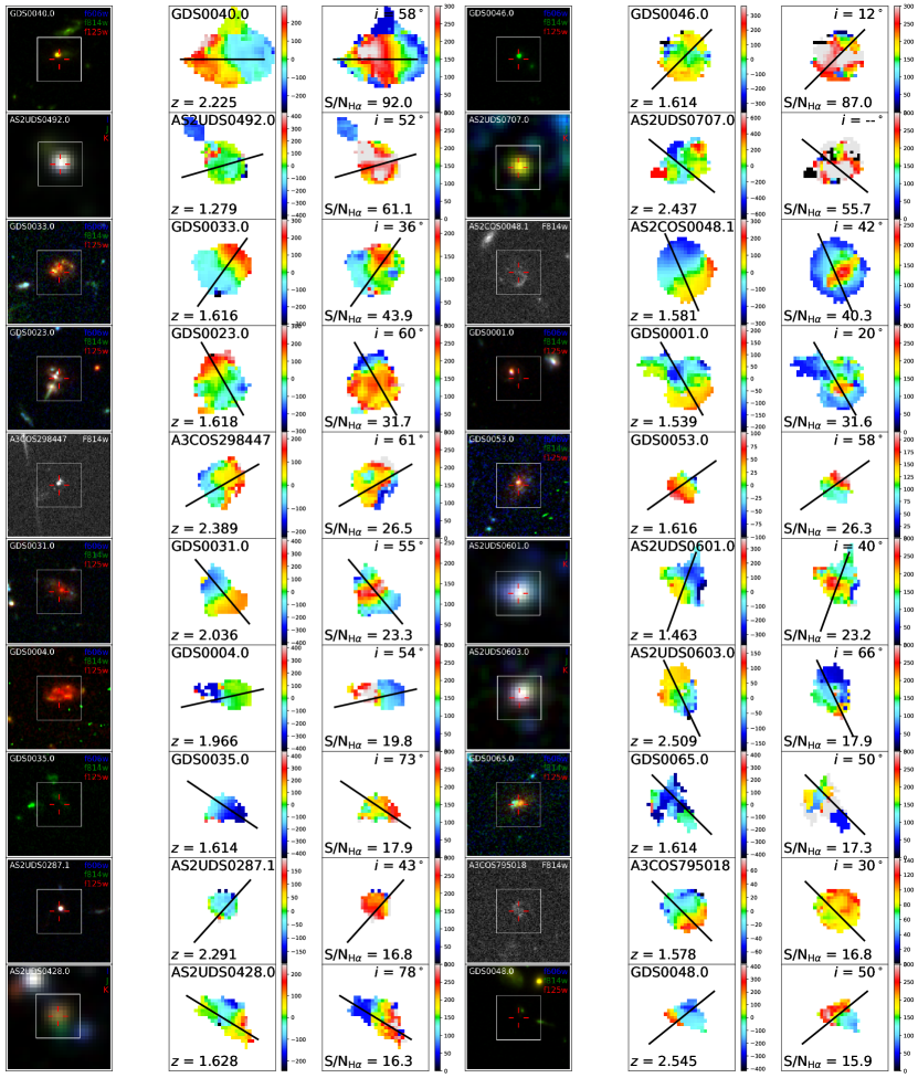
Figure 2: HST F160W or ground-based $K$-band images (left), velocity fields (middle) and velocity dispersion profiles (right) for our sample of 31 resolved KAOSS DSFGs. The images are 7.5^′′ $\times$ 7.5^′′ in size, and the white box indicates the region shown in the velocity and velocity dispersion maps (3.2^′′ $\times$ 3.2^′′ in size). Sources are ordered by the S/N of the H$\alpha$ emission line (shown in the bottom-left corner of the middle panels) and we indicate the inclination angle derived for the source from galfit modelling. The black lines on the centre and right panels indicate the kinematic position angle along which rotation curves are measured. For the left panels we indicate the three filters that make up the RGB colour image, or the single filter in cases where the image is greyscale.

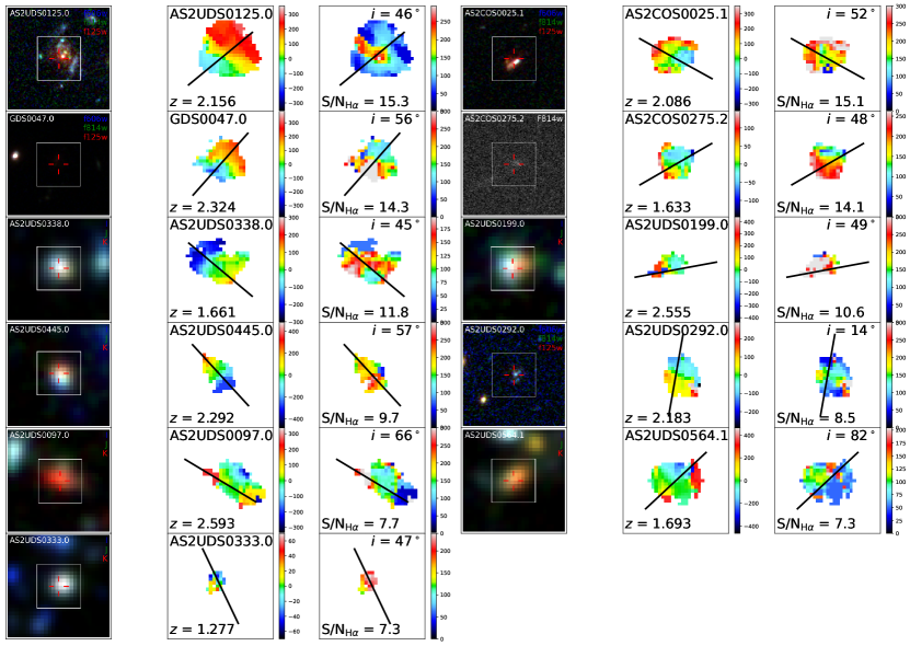
Figure 3 (Cont.):

We fit a three-component Gaussian profile, plus a constant continuum component, to the H$\alpha$ line and [Nii]$\lambda\lambda$6548,6583 doublet, coupling their wavelengths and linewidths, with the [Nii]$\lambda 6583$/H$\alpha$ flux ratio as a free parameter, and fixing the [Nii]$\lambda 6583$/[Nii]$\lambda 6548$ flux ratio to a value of 2.8 (Osterbrock & Ferland, 2006). We perform the fitting over the region of the spectra within $\pm$ 0.02 $\mu$m of the H$\alpha$ emission line. Observed linewidths are deconvolved with the instrumental resolution, as determined by fitting several sky lines over the $HK$ band, to calculate the intrinsic linewidths.

We perform the fitting on a pixel-by-pixel basis, first resampling the velocity fields from a spatial pixel scale of 0.2^′′ to 0.1^′′, enabling us to sample finer spatial scales. For each pixel we attempt to fit the emission lines, and if the fit does not achieve a threshold of S/N $=$ 5 we bin with neighbouring pixels, increasing the bin size and repeating up to a maximum bin size of 5 pixels (0.5^′′) or until the S/N threshold is achieved. For the systemic redshifts we use the values derived from fits to the integrated spectra (Birkin et al. in prep.).

Velocity and velocity dispersion maps for all the galaxies in the resolved sample are shown in Fig. 2 alongside rest-frame optical colour images of the sources. For the colour images we include high-resolution HST imaging where possible, otherwise we use ground-based imaging. Sources are ordered by the integrated S/N of the H$\alpha$ emission line which generally correlates with the quality of the kinematic information from the fitting. Several of the sources in Fig. 2 display smooth H$\alpha$ velocity gradients, such as AS2COS0048.1, GDS0033.0 and GDS0031.0, which indicate ordered rotation in these galaxies. Others, such as GDS0001.0, GDS0046.0 and AS2UDS0428.0, display more turbulent, complex velocity structures and morphologies.

The source AS2UDS0492.0 is unique in our sample, since we detect velocity structure from a separate component to the north west within the 2.8^′′ field of the KMOS IFU – this component is detected in the ground-based near-infrared imaging (see Fig. 2) and corresponds to a companion galaxy. This particular source also displays a broad component in the H$\alpha$ emission, AGN-like IRAC colours and has an X-ray component. The fit to the H$\alpha$ emission in AS2UDS0707.0 is poor despite the high S/N of the integrated emission (S/N${}_{{\rm H}\alpha}\sim$ 56). Like AS2UDS0492.0, this source displays broad H$\alpha$ emission, but it also has a very low [Nii]/H$\alpha$ flux ratio.

The velocity dispersion maps in Fig. 2 generally appear structured, even for the sources with the most significant detections, for example AS2UDS0707.0, AS2COS0025.1 and AS2UDS0338.0. Given the compact sizes of our sources (median $R_{\rm e}$ $\sim$ 0.4^′′) relative to the KMOS PSF (FWHM $\sim$ 0.6^′′) our observations are susceptible to the effects of beam smearing, leading to increased observed velocity dispersions in the centres of galaxies and flattening of their observed rotation curves (e.g. Johnson et al., 2018). However, it can be seen in sources such as AS2COS0048.1 and AS2UDS0125.0 that we resolve the H$\alpha$ emission on scales large enough to reach the point where the velocity dispersion profile flattens out. We provide a discussion of beam smearing in our sample and the methods with which we account for it in §4.3.

3.4 Spectral energy distribution fitting

To estimate physical properties for our sources we fit their SEDs employing the high-$z$ version of the magphys code, fixing the redshift to the KMOS spectroscopic value. We direct the reader to Birkin et al. (2021) for a thorough description of our methods for SED fitting with magphys, but we note here that, of the 31 sources in the resolved sample, 28 (90 per cent) have Spitzer/MIPS 24-$\mu$m detections and 29 (94 per cent) have at least one Herschel/SPIRE detection. All sources are detected at 870 $\mu$m. The photometry used for each of the three fields is as follows:

• COSMOS: CFHT Megacam $U$, Subaru SuprimeCam $BVRIz$, Subaru HSC $Y$, VISTA $HK_{s}$, Spitzer IRAC1-4 (Laigle et al., 2016), Spitzer MIPS 24$\mu$m, Herschel PACS 100$\mu$m, 160$\mu$m, Herschel
  SPIRE 250$\mu$m, 350$\mu$m, 500$\mu$m (Jin et al., 2018), ALMA 870$\mu$m
  (Simpson et al., 2020) and VLA 3 GHz (Smolčić et al., 2017)

• UDS: CFHT Megacam $U$, Subaru SuprimeCam $BVRIz$, VISTA $Y$, UKIRT WFCAM $JHK$ (Lawrence et al., 2007), Spitzer IRAC1-4, Spitzer MIPS 24$\mu$m (Kim et al., 2011), Herschel PACS 100$\mu$m,
  160$\mu$m, Herschel SPIRE 250$\mu$m, 350$\mu$m, 500$\mu$m (Oliver et al., 2012),
  ALMA 870$\mu$m (Stach et al., 2019) and VLA 1.4 GHz (Simpson et al., 2013)

• GOODS-S: VIMOS $U$, HST ACS F435W, F606W, F775W, F814W, F850LP, HST WFC3 F098M, F105W, F125W, F160W, VLT/HAWK-I $K_{s}$, Spitzer IRAC1-4 (Guo et al., 2013), Spitzer MIPS 24$\mu$m (Giavalisco et al., 2004), Herschel PACS 70$\mu$m, 100$\mu$m, 160$\mu$m, Herschel SPIRE 250$\mu$m, 350$\mu$m, 500$\mu$m (Elbaz et al., 2011), ALMA 870$\mu$m (Cowie et al., 2018; Liu et al., 2019) and VLA 1.4 GHz (Miller et al., 2013).

The observed fluxes or limits and the corresponding best-fit magphys SEDs for the 31 KAOSS DSFGs are shown as a figure in the online supplementary material. magphys provides a good fit to the observed photometry in all cases. We note here, however, that the high-$z$ version of magphys does not include contributions to the continuum emission from an AGN. The effects of this on DSFG stellar mass estimates from magphys have been tested in Birkin et al. (2021), where it was found that $M_{\ast}$ may be modestly overestimated by the fitting code, although we do not expect this to effect our conclusions.

The best-fit SED parameters and their uncertainties are shown in the online supplementary table, but here we report that the 31 resolved KAOSS DSFGs have median values of $M_{\ast}=(1.3\pm 0.2)\times 10^{11}$ M_⊙, $M_{\rm dust}=(4.9\pm 0.9)\times 10^{8}$ M_⊙, SFR $=$ 220 $\pm$ 30 M_⊙ yr^-1, $L_{\rm IR}=(2.5\pm 0.4)\times 10^{12}$ L_⊙ and $A_{V}=2.14\pm 0.14$.

3.5 galfit modelling

When deriving rotational velocities and dynamical masses it is key to estimate the inclination and size of the galaxy. To do this for the KAOSS galaxies we exploit existing HST/F160W imaging for 14 of the 31 DSFGs, and ground-based $K$-band imaging from: VISTA for COSMOS (McCracken et al., 2012, seeing $\sim$ 0.8^′′), UKIRT WFCAM for UDS sources (Almaini et al. in prep.), and HAWK-I for GOODS-S sources (Fontana et al., 2014, seeing $\sim$ 0.4^′′); for the remaining 17. We fit the 2-D continuum with Sérsic profiles using the galfit code (Peng et al., 2010), constraining the Sérsic index $n$ to be between 0.5 and 4, and allowing the effective radius $R_{e}$, axis ratio $b$/$a$ and position angle (PA) to vary. We visually inspect all fits and flag sources where we are unable to find a model that reproduces the source structure, or where the best-fit parameters are unphysical (for example, effective radii of $\ll$ 1 pixel), although this is only necessary for three sources (GDS0046.0, AS2UDS0707.0 and AS2UDS0287.1). The median Sérsic index of the entire sample is $n$ $=$ 1.00 $\pm$ 0.16 from the fits with $n$ as a free parameter, i.e. consistent with an exponential profile, and we therefore repeat the fitting fixing $n$ $=$ 1, following Gullberg et al. (2019).

As a test of the suitability of lower-resolution ground-based $K$-band imaging we compare measurements of $R_{\rm e}$ and $b$/$a$ from ground-based $K$-band and HST/F160W imaging for the 13 sources with coverage in both bands, fitting a fixed $n$ $=$ 1 profile in both cases. We find that the two are consistent for these sources, and we therefore suggest that size and $b$/$a$ measurements from ground-based $K$-band imaging are acceptable in the absence of HST/F160W imaging.

In order to estimate uncertainties on the galfit parameters we simulate Sérsic profiles with known properties at different signal-to-noise ratios. We do this for two cases, one with PSFs comparable to the $K$-band imaging and one comparable to the HST/F160W imaging. Finally, we calculate the dispersion in the measurements at different S/N. As a result of these simulations we elect to adopt a constant 10 per cent uncertainty for all measurements of $R_{\rm e}$ and $b/a$, which we find to be generally conservative for the typical S/N levels of the optical/NIR imaging (see Birkin, 2022, for more details).

To estimate inclination angles we use the best-fitting galfit parameters as follows:

$$\cos(i)=\sqrt{\dfrac{(b/a)^{2}-(b/a)_{0}^{2}}{1-(b/a)_{0}^{2}}},$$ (1)

where $(b/a)_{0}$ accounts for the fact that the discs have a finite thickness – we adopt $(b/a)_{0}$ $=$ 0.2, following Gillman et al. (2019) and other similar surveys such as KROSS (Stott et al., 2016) and KGES (Gillman et al., 2020), for consistency. Our sample has a median axial ratio of $b/a$ $=$ 0.64 $\pm$ 0.03 and a median derived inclination of $i$ $=$ 54 $\pm$ 3 ^∘, consistent with the prediction of 57^∘ for randomly oriented thin discs (Law et al., 2009).

3.6 JWST/NIRCam imaging

One of the sources in the resolved sample, AS2UDS0125.0 ($z$ $=$ 2.156), has been imaged with JWST NIRCam (Proposal ID 1837, PI J. Dunlop), which represents a significant improvement on the wavelength coverage and sensitivity of the existing HST imaging.

Therefore, in Fig. 4 we show cutouts of this source in NIRCam bands F090W, F115W, F150W, F200W, F277W, F356W, F410M and F444W, alongside a HST colour image (F606W/F814W/F125W). The NIRCam imaging clearly shows clumpy, spiral arm-like structures which are suggested in the HST imaging. AS2UDS0125.0 therefore appears to be disc like from the morphology of the stellar continuum, which is in agreement with the apparent velocity gradient and measured value of $v_{\rm rot}/\sigma_{0}$ $=$ 3.6 $\pm$ 0.4 (see §4).

While this is the only source in our sample which currently has NIRCam coverage, we can already see the enormous potential of JWST for advancing our understanding of the DSFG population.

Figure 4: 7.5^′′ $\times$ 7.5^′′ cutouts of AS2UDS0125.0 in JWST/NIRCam bands F090W, F115W, F150W, F200W, F277W, F356W, F410M and F444W, alongside a HST colour image of the same source. The NIRCam imaging shows clear clumpy spiral arm structures which begin to emerge in the F115W filter ($\lambda_{\rm rest}$ $\sim$ 0.36 $\mu$m). We note that the NIRCam imaging is rotated by approximately 20^∘ anticlockwise with respect to the HST imaging.

3.7 Determining rotation axes

To quantify the kinematic structure of our sample, we need to parameterise the dynamics through measurements of the rotational velocity, $v_{2.2R_{\rm d}}$, and velocity dispersion, $\sigma_{\rm obs}$. These quantities can be estimated from the rotation curves and velocity dispersion profiles as extracted from the kinematic maps derived in §3.3. First we determine the axes across which our sources have the largest velocity gradient. One way to assess this axis is to use the morphological major axis derived in §3.5, PA_morph. Alternatively we can use the velocity field itself to estimate a kinematic axis, PA_kin.

To determine PA_kin it is necessary to ensure that the velocity fields are appropriately centred, for which we employ the following method. First, we attempt to measure a centroid from the continuum image of the source constructed from the collapsed KMOS cube. If the continuum is not detected, we next measure a centroid from the H$\alpha$ image. In the event that both of these methods are unsuccessful (i.e. if the H$\alpha$ S/N is low) we visually inspect the velocity field to determine its center. In total we measure centroids for 23, 4 and 4 sources for the three methods, respectively. We then shift the velocity field to align it with the chosen centroid, corresponding to a median shift of 0.40^′′ $\pm$ 0.06^′′.

Figure 5: Misalignment between the position angle derived from H$\alpha$ kinematics (PA_kin) and the position angle derived from optical/NIR imaging (PA_morph), versus axis ratio $b/a$. PA_morph and $b/a$ are both measured from galfit modelling of high-resolution optical/NIR imaging (see §3.5). The horizontal dashed line indicates a misalignment of 30^∘, less than which are taken to be reasonable agreement between the two PAs. In the top-left corner we show a representative error bar for KAOSS galaxies, and as a comparison sample we plot results from the KROSS survey of SFGs at $z$ $\sim$ 1 (Harrison et al., 2017). A Kolmogorov-Smirnov test shows that the two distributions are consistent with having been drawn from the same parent sample at the 95 per cent confidence level, indicating that the KAOSS resolved sample shows similar levels of kinematic misalignment to “main-sequence” galaxies at $z$ $\sim$ 1.

Having centred our velocity fields we then determine their rotational axes (or kinematic position axes; PA_kin) using two methods. First, we place a pseudo-slit across the velocity field and measure the peak-to-peak difference in velocity, $\Delta v$, then rotate the pseudo-slit through to determine $\Delta v$ as a function of $\theta$, from which we find the angles that both maximise and minimise $\Delta v$: $\theta_{\Delta v_{\rm max}}$ and $\theta_{\Delta v_{\rm min}}$. Finally we use

$${\rm PA}_{\rm kin}=\dfrac{\theta_{\Delta v_{\rm max}}+(\theta_{\Delta v_{\rm min}}+90^{\circ})}{2}$$ (2)

to derive the PA_kin. To estimate uncertainties on the PA_kin we employ a Monte Carlo technique, randomly resampling the velocity fields 100 times using the measurement uncertainties, and measuring the spread in the distribution of the resultant 100 values.

When the S/N of the emission is low, this method is noisy and the resulting PA_kin may not appear to correlate well with the velocity field. Hence, in all cases we also identify a maximum velocity gradient PA_kin by eye, and where the PA_kin chosen by the algorithm described above does not appear to be a good fit to the velocity field (which we assess visually) we simply use the “by eye” PA_kin. For context, we use the visual estimate of PA_kin for 13 (typically lower S/N) out of the 31 sources in the sample. For these sources we adopt an uncertainty of $\pm$ 5^∘, which is comparable to the median uncertainty estimated from the 18 sources with Monte Carlo-derived uncertainties, as described above. Our best-estimated values of the PA are tabulated in the online supplementary table, and in Fig. 2 we overlay PA_kin on both the velocity and velocity dispersion maps.

For galaxies that are highly inclined, the kinematic and morphological position angles should be consistent (i.e. PA_kin $=$ PA_morph), however in systems that are kinematically and morphologically complex this is not necessarily true. Comparing the two position angles therefore provides another metric for identifying disturbed systems (e.g. Wisnioski et al., 2015; Harrison et al., 2017). In Fig. 5 we show the misalignment between the kinematic position angle PA_kin and the morphological position angle measured from the galfit modelling of the optical/NIR imaging, PA_morph (see §3.5), as a function of the major-to-minor axis ratio $b/a$ (also derived from galfit, see §3.5). We indicate a misalignment of 30^∘ following Wisnioski et al. (2015), finding that ten galaxies lie above this threshold and 21 below it. Therefore, 32 $\pm$ 10 per cent of the resolved KAOSS DSFGs display kinematic and morphological axes that are misaligned by more than 30^∘.

As a comparison sample we also show the distribution of galaxies from the $z$ $\sim$ 1 KROSS star-forming galaxy sample (Harrison et al., 2017), with histograms of the distributions shown on both axes. We perform a two-sample Kolmogorov-Smirmov (K–S) test between the distributions of both the PA offsets and the axial ratios from KAOSS and KROSS, finding them both to be consistent with being drawn from the same parent population at the 95 per cent confidence level. The KROSS sample is comprised of main-sequence star-forming galaxies at $z$ $\sim$ 1, with typical star-formation rates of $\sim$ 7 M_⊙ yr^-1, and this suggests that our sample is no more kinematically complex than much less-active SFGs, in terms of the axial misalignment. Later in our analysis we will further test this result by comparing the star-formation rates and velocity dispersions of different samples.

3.8 AGN classification

To place our results in context with other DSFGs, and with star-forming galaxies in general, it is important to first understand the fraction of sources with active galactic nuclei (AGN) in our sample. We expect this to be moderate – the largest sample of 870 $\mu$m-selected DSFGs (also one of the main parent samples for KAOSS), the AS2UDS sample, contains an estimated 18 $\pm$ 10 per cent sources with AGN components based on X-ray and photometric tests (Stach et al., 2019). Our rest-frame optical spectra allows us to also search for spectral indications of AGN. Therefore to provide a census of AGN in our sample we assess how many sources meet the following criteria:

• flux ratio [Nii]$\lambda$6583/H$\alpha$ $>$ 0.8 (e.g. Wisnioski et al., 2018);

• H$\alpha$ emission displays a broad component with a linewidth of FWHM $>$ 1000 km s^-1 (e.g. Genzel et al., 2014);

• presence of a luminous X-ray counterpart ($L_{\rm X}$ $\geq$ 10⁴² erg s^-1) matched within 1^′′ (Civano et al., 2016; Luo et al., 2017; Franco et al., 2018; Kocevski et al., 2018);

• Spitzer IRAC colours indicating an AGN according to the criteria of Donley et al. (2012).

In total 18 of the sample of 31 sources fit one or more of these criteria, indicating an AGN fraction of 58 $\pm$ 14 per cent. This is significantly higher than the range quoted for the AS2UDS sample in Stach et al. (2019), but we expect a bias towards detecting AGN in our sample given the fact that such sources display stronger emission lines. Additionally, this should be treated as an upper limit given that some sources may meet the criteria for other reasons, for example high [Nii]/H$\alpha$ ratios may also arise from high metallicities (e.g. Allen et al., 2008; Kewley & Ellison, 2008). Tellingly, only two sources meet all four criteria, these are AS2UDS0492.0 and AS2UDS0287.1.

We separate potential AGN-host sources into two categories: those that are classified as hosting AGN based on their rest-frame optical spectra, and those that are classified as hosting AGN based on their X-ray and/or IRAC properties. In the former case we include the 12 sources (39 $\pm$ 11 per cent of the sample) that have [Nii]/H$\alpha$ $>$ 0.8 or FWHM${}_{{\rm H}\alpha}>$ 1000 km s^-1. In the latter category we find 16 sources (52 $\pm$ 13 per cent), including ten that are also in the spectral AGN sample. In all plots that follow we flag AGN-classified DSFGs with a star symbol, with the star-forming sources shown as circular points.

4 Results and discussion

We have identified a sample of 31 DSFGs with spatially resolved emission line maps, yielding velocity and velocity dispersion maps, along with their physical properties from SED fitting. Additionally, we have identified and flagged which of the sources exhibit properties that suggest a contribution to the emission from an AGN. We now turn to deriving the rotational velocities and intrinsic velocities of the sample, and eventually the ratio of these two quantities, which is suggested to be a diagnostic of the level of rotational support. We study the variation of these properties with other important variables such as SFR and $M_{\ast}$, before placing our sample within the context of the Tully-Fisher relation, and estimating their halo masses, which we use to study the stellar-to-halo mass relation (SHMR) for DSFGs.

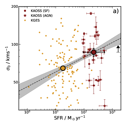
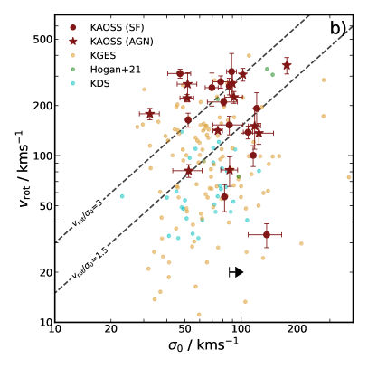
Figure 6: a) Intrinsic velocity dispersion $\sigma_{0}$ versus magphys-derived star-formation rates for the KAOSS and KGES samples. The KAOSS resolved sample has SFRs that are roughly an order of magnitude higher than the KGES sample, and we see a positive trend in $\sigma_{0}$ with SFR (and hence that more actively star-forming galaxies are more turbulent). We note that the “error bar” on the abscissa on the KAOSS median point represents the range in SFR spanned by the bin, and this is also the case in subsequent plots. b) Rotational velocity $v_{\rm rot}$ versus intrinsic velocity dispersion $\sigma_{0}$ for the KAOSS disc-like sample along with the KGES, Hogan et al. (2021) and KDS samples. We indicate lines of constant $v_{\rm rot}/\sigma_{0}$ $=$ 1.5 and 3, two potential lower limits on a system being rotationally supported. In general, the KAOSS DSFGs are both more rapidly rotating and more turbulent than the other samples, which results in only slightly higher $v_{\rm rot}/\sigma_{0}$ than those galaxies. This result is important as it shows that both $v_{\rm rot}$ and $\sigma_{0}$ are driving the variation of $v_{\rm rot}/\sigma_{0}$ in DSFGs with respect to other galaxy populations.

4.1 Rotation curve modelling

From our derived resolved velocity maps (see §3.3) we extract rotation curves and velocity dispersions profiles. Rotation curves are extracted from the velocity field within a 0.5^′′ wide ($N$ = 5 pixels in the rebinned cube) pseudo-slit along the PA_kin from the velocity field, taking the median of the pixels across the slit. Velocity dispersion profiles are extracted from the velocity dispersion maps using the same slit, and uncertainties are extracted from the corresponding uncertainty maps. The resultant rotation curves are shown in the left panels of Fig. 13. We note that the velocities plotted are those directly measured from the velocity maps, and no inclination corrections are applied at this stage.

In order to derive rotational velocities we fit the rotation curves with a model of the form (Freeman, 1970):

$$(v(r)-v_{\rm off})^{2}=\dfrac{(r-r_{\rm off})^{2}\pi G\mu_{0}}{h}(I_{0}K_{0}-I_{1}K_{1}),$$ (3)

following Harrison et al. (2017) and Tiley et al. (2021), where $v$ is the velocity in km s^-1, $r$ is the radial distance from the centre along the rotation axis in kpc, $v_{\rm off}$ if the velocity offset of the rotation curve from the nominal systemic redshift (derived from the integrated spectra), $r_{\rm off}$ is the spatial offset of the selected centroid from the spatial position of the systemic velocity on the rotation curve, $\mu_{0}$ is the peak mass surface density, $h$ is the disc scale radius and $I_{n}K_{n}$ are Bessel functions evaluated at 0.5$r/h$. We see in Fig. 13 that this model is a reasonably good fit to the data for 25 of the 31 sources (81 $\pm$ 16 per cent), which we term the disc-like sample. The best-fit parameters $v_{\rm off}$ and $r_{\rm off}$ are tabulated in the online supplementary table.

For the six sources which we are poorly fit by the Freeman disc model we are unable to estimate a robust rotational velocity. Therefore, we attempt to assess whether there are any obvious intrinsic differences in the physical properties of these six sources with the 25 disc-like sources. Examining median values for the two subsamples, the disc-like and poorly fit samples have consistent stellar masses, $M_{\ast}$ $=$ (1.3 $\pm$ 0.2) $\times$ 10¹¹ M_⊙ and $M_{\ast}$ $=$ (2.3 $\pm$ 1.8) $\times$ 10¹¹ M_⊙, consistent star-formation rates, SFR $=$ 220 $\pm$ 30 M_⊙ yr^-1 and SFR $=$ 210 $\pm$ 90 M_⊙ yr^-1, and consistent dust extinctions, $A_{V}$ $=$ 2.01 $\pm$ 0.16 and $A_{V}$ $=$ 2.4 $\pm$ 0.5, respectively. We therefore find no significant difference between the two subsets in terms of their physical properties.

Additionally, we test for differences in the integrated S/N of the H$\alpha$ emission and $K$-band magnitudes of the two samples, respectively finding median S/N $=$ 18 $\pm$ 3 and S/N $=$ 16 $\pm$ 7, and $K$ $=$ 21.4 $\pm$ 0.2 and $K$ $=$ 21.2 $\pm$ 0.3. Therefore neither of these observed properties show any significant difference. Given these findings, we elect to focus the remainder of our analysis on the 25 sources with robust rotational velocity measurements, and suggest that the six poorly fit systems are systematically comparable to the disc-like sources, therefore omitting them should not significantly bias our conclusions.

4.2 Inclination corrected rotational velocities

As a measure of the rotational velocity of each galaxy we evaluate $v_{\rm rot}$ $=$ $v_{2.2R_{\rm d}}$ / $\sin{i}$, where $v_{2.2R_{\rm d}}$ is the observed velocity at 2.2 $R_{\rm d}$ according to the model fits and the factor of 1 / $\sin{i}$ corrects for the observed inclination of the source. The inclination angle $i$ is measured from galfit modelling (see §3.5, and the online supplementary table).

We note that as some of the derived inclination angles are apparently small ($<$ 20^∘) we set a minimum inclination of $i$ $=$ 20^∘, to avoid significant extrapolations (given the simple models we are adopting). This only affects two sources, GDS0046.0 and AS2UDS0292.0, which have galfit-derived inclinations of $i$ $=$ 12^∘ $\pm$ 17^∘ and $i$ $=$ 14^∘ $\pm$ 15^∘ respectively. Both are consistent with our chosen minimum inclination (20^∘) within their large uncertainties. Additionally, the axis ratio measured from galfit for AS2UDS0707.0 is less than $(b/a)_{0}$ (for which we adopted a value of 0.2, see §3.5), resulting in an unphysical inclination angle; we also set a minimum inclination of $i$ $=$ 20^∘ for this source.

After applying inclination corrections we derive a median rotational velocity of $v_{\rm rot}$ $=$ 190 $\pm$ 30 km s^-1 for the disc-like sources. For context, the $z$ $\sim$ 1.5 KGES sample has a median inclination-corrected velocity at 2.2 $R_{\rm d}$ of 61 $\pm$ 5 km s^-1, and the $z$ $\sim$ 1 KROSS sample has a median inclination-corrected velocity at 2.2 $R_{\rm d}$ of 109 $\pm$ 5 km s^-1, both of which are significantly lower than the corresponding value for the KAOSS disc-like sample. We conclude that KAOSS DSFGs have much higher rotational velocities than less active (and apparently lower mass) galaxies that have been observed with KMOS.

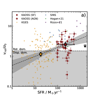
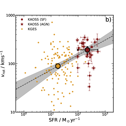
Figure 7: a) Ratio of rotational velocity to velocity dispersion $v_{\rm rot}/\sigma_{0}$ versus SFR. Also shown are $z$ $\sim$ 1.5 galaxies from the KGES survey, $z$ $\sim$ 1.3–2.6 galaxies from SINS and $z$ $\sim$ 4.5 DSFGs from Rizzo et al. (2021). We fit the binned KAOSS and KGES median points (large circles with black outline), finding a weak (2.8$\sigma$) correlation between $v_{\rm rot}/\sigma_{0}$ and SFR (black dashed line with grey uncertainty region). The arrow shows how far the points would move down if we were to remove the beam smearing corrections to the velocity dispersions. b) Rotational velocity $v_{\rm rot}$ versus SFR for the KAOSS and KGES samples. We measure a 4.1$\sigma$ correlation between $v_{\rm rot}$ and SFR from the fit to the binned data (black dashed line with grey uncertainty region), which we suggest is driven by the “main-sequence” correlation between SFR and stellar mass, leading to higher SFRs in galaxies with greater stellar masses and therefore faster rotation velocities.

4.3 Observed velocity dispersions and beam smearing corrections

We now turn to measuring the velocity dispersions in our sources, which will allow us to assess the degree of turbulent motion in DSFGs. To measure the observed velocity dispersion, $\sigma_{\rm obs}$, we inspect the velocity dispersion profiles (Fig. 13) and divide them into two groups, following Johnson et al. (2018): first, where the velocity dispersion appears to have flattened in the outskirts, we measure $\sigma_{\rm obs}$ as the median of the three outer points (spanning 0.3^′′ or $\sim$ 2.5 kpc) on both sides and take the lower value of the two sides. In all other cases we simply measure $\sigma_{\rm obs}$ as the median of the dispersion profile. As in Johnson et al. (2018) we label the sources “O” and “M” (see Fig. 13) to indicate that the intrinsic velocity dispersion has been measured from the “outskirts” or “median”, respectively. For the 31 resolved sources, we measure $\sigma_{\rm obs}$ from the outskirts in 16 cases, and from the median in the remaining 15 cases.

As noted in §3.3, our estimates of the rotational velocity and velocity dispersion are affected by beam smearing, which results in an increased velocity dispersion near the centre of the galaxy. To correct for this effect and obtain estimates of the intrinsic velocity dispersion $\sigma_{0}$ we use the prescriptions of Johnson et al. (2018), who derived correction factors from mock KMOS observations for the KROSS survey. For specific details on the corrections we direct the reader to Johnson et al. (2018), but we note here that they are dependent on the size and rotational velocity of the galaxy. For the former we adopt the median $R_{\rm d}$ of our sample from the galfit measurements for all sources, $R_{\rm d}$ $=$ 0.4 $\pm$ 0.05^′′, and for the latter we use the observed velocity at 2.2 $R_{d}$. Observed and intrinsic velocity dispersions, $\sigma_{\rm obs}$ and $\sigma_{0}$, are listed in the online supplementary table.

For the 15 sources in the median (“M”) subset the median beam smearing correction is $\xi_{\sigma,{\rm M}}$ $=$ 0.63 $\pm$ 0.06, and for the 16 sources in the outskirts (“O”) subset the median beam smearing correction is $\xi_{\sigma,{\rm O}}$ $=$ 0.96 $\pm$ 0.02. This demonstrates that the effects of beam smearing are much less severe in the outskirts of the galaxy. The value for the “O” subset is comparable to the corrections used for KROSS by Johnson et al. (2018) who found $\xi_{\sigma,{\rm O}}$ $=$ 0.96${}^{+0.02}_{-0.06}$ for outskirt $\sigma$ measurements, but they applied a much less significant correction than we do, $\xi_{\sigma,{\rm M}}$ $=$ 0.8${}^{+0.1}_{-0.3}$ for median $\sigma$ measurements.

Investigating the cause of this difference, the KAOSS sources are marginally larger than the KROSS sources, median $R_{\rm e}$ $=$ 3.6 $\pm$ 0.3 kpc for KAOSS compared to median $R_{\rm e}$ $=$ 2.9${}_{-1.5}^{+1.8}$ kpc (Harrison et al., 2017) for KROSS (both surveys have comparable seeing). However, the KAOSS galaxies have much higher rotational velocities, with a median $v_{\rm rot}$ $=$ 190 $\pm$ 30 km s^-1 compared to a median $v_{\rm rot}$ $=$ 109 $\pm$ 5 km s^-1 from KROSS (Harrison et al., 2017). Therefore the KAOSS sources experience stronger beam smearing than those of KROSS due to the much larger rotational velocities of the galaxies.

We also apply beam-smearing corrections to the rotation velocities, $\xi_{v}$, following Johnson et al. (2018), although these corrections are generally much smaller. Our sample has a median rotational velocity correction of $\xi_{v}$ $=$ 1.06 $\pm$ 0.01, increasing the median $v_{\rm rot}$ by $\sim$ 11 km s^-1. This is also consistent with the corrections applied by Johnson et al. (2018) to the KROSS sample, who found a median $\xi_{v}$ $=$ 1.07 $\pm$ 0.03.

We caution that our use of the beam-smearing corrections from Johnson et al. (2018) are based on the assumption that the resolved KAOSS sources can be described by rotating discs, which is a simplistic assumption for DSFGs given that they may be kinematically more complex, as discussed earlier (see also e.g. Alaghband-Zadeh et al., 2012). We therefore add vectors to all figures that show quantities derived using $\sigma_{0}$ to illustrate how the plotted values would change if we had applied no beam-smearing correction. The “true” intrinsic velocity dispersions are likely to lie somewhere between no correction and the full correction. As the corrections to $v_{\rm rot}$ are small ($\sim$ 5 per cent) we do not add similar vectors to plots including the rotational velocity.

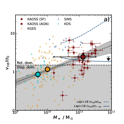
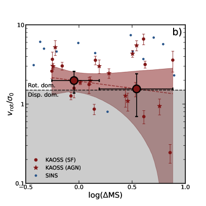
Figure 8: a) Ratio of rotational velocity to velocity dispersion $v_{\rm rot}/\sigma_{0}$ versus stellar mass, with the same galaxy samples as in the previous figure, with the addition of $z$ $\sim$ 3.5 galaxies from the KMOS Deep Survey (Turner et al., 2017). We include two tracks from simulations of early-type galaxy progenitors (Lapi et al., 2018), with $v_{\rm rot}/\sigma_{0}$ measured at the centrifugal size of the gas (dashed) and stellar (solid) components. Our data are in reasonable agreement with the latter and are therefore consistent with the predictions of $v_{\rm rot}/\sigma_{0}$ for early-type progenitors. b) Ratio of rotational velocity to velocity dispersion $v_{\rm rot}/\sigma_{0}$ offset from the main sequence ($\Delta$MS) for KAOSS and SINS sources. The dark grey region shows the $\pm$ 0.3 dex scatter of the main sequence. We fit our binned data (black dashed line), which shows virtually no correlation between the two properties, suggesting that “starburst”-like sources do not show more turbulent support than regular disc-like sources.

4.4 Intrinsic velocity dispersions

The intrinsic velocity dispersions $\sigma_{0}$ we have derived provide a measure of how turbulent our DSFGs are, and we can compare these values to those measured from other galaxy populations to determine the relative level of turbulence as a function of galaxy parameters such as rotational velocity and star-formation rate.

Our sample has a median $\sigma_{\rm obs}$ $=$ 111 $\pm$ 18 km s^-1, and a median $\sigma_{0}$ $=$ 87 $\pm$ 6 km s^-1. The Hogan et al. (2021) and Alaghband-Zadeh et al. (2012) samples, which are similarly selected, have median intrinsic velocity dispersions of $\sigma_{0}$ $=$100 $\pm$ 20 km s^-1 and $\sigma_{0}$ $=$160 $\pm$ 60 km s^-1, respectively, both of which are comparable with the KAOSS sample. On the other hand the KGES sample has a median beam smearing-corrected velocity dispersion of $\sigma_{0}$ $=$ 46 $\pm$ 2 km s^-1 (Tiley et al., 2021). Hence the dust-obscured and typically strongly star-forming KAOSS sources have systematically higher intrinsic velocity dispersions, and are therefore apparently more turbulent than the KGES galaxies.

Determining the origin of the turbulence is difficult, and we do not attempt to do this quantitatively here. Distinct kinematic components in our data would indicate ongoing interactions, which would likely produce high levels of turbulence from tidal flows between the two systems, but our data do not reveal such components beyond the $\sim$ 42 per cent of the sample that are not well described by disc-like kinematics. It is possible that AO-assisted SINFONI/ERIS or JWST/NIRSpec observations would uncover interactions, as they would more easily probe $\sim$ 1 kpc scales. Alternatively, star formation itself may induce the turbulence, or cold accretion flows from the IGM, which may trigger the release of large amounts of gravitational energy (Genzel et al., 2008).

To quantify this further, in Fig. 6 we show $\sigma_{0}$ versus star-formation rate, as measured from magphys SED fitting. The KAOSS DSFGs have an order of magnitude higher star-formation rates than the KGES sample, and we again see that KAOSS galaxies display higher velocity dispersions, whether corrected or uncorrected for beam smearing. We fit the median KAOSS and KGES points (with bootstrap uncertainties), finding a 5.3$\sigma$ correlation between $\sigma_{0}$ and SFR, indicating a modest link between the two quantities. Therefore the high SFRs could produce the observed turbulence, but we interpret this result with caution given the different selections of the two samples.

4.5 Rotational support

Having determined that KAOSS DSFGs are apparently turbulent and massive sources, we now assess whether turbulence is the dominant source of motion. One of the simplest methods of doing this is to calculate the ratio of rotation velocity to intrinsic velocity dispersion $v_{\rm rot}/\sigma_{0}$ (e.g. Weiner et al., 2006; Wisnioski et al., 2015): if a galaxy has a much higher rotation velocity than its velocity dispersion then it is considered to be “rotationally supported”. Alternatively a galaxy that appears to be dominated by turbulent motions may be displaying inclination or projection effects, and/or may be supported through ongoing interactions or mergers.

Before deriving $v_{\rm rot}/\sigma_{0}$ we show the intrinsic velocity dispersion $\sigma_{0}$ as a function of the rotational velocity $v_{\rm rot}$ for the resolved KAOSS sources in Fig. 6, alongside galaxies from the KGES sample and Hogan et al. (2021). This demonstrates the elevated rotational velocities and velocity dispersions of the KAOSS sources compared to the KGES sample that were discussed in §4.1 and §4.4.

Among the sources in our sample with robust $v_{\rm rot}$ measurements, 18 of the 25 sources (72 $\pm$ 17 per cent) fit the criterion for rotationally dominated sources of $v_{\rm rot}/\sigma_{0}$ $>$ 1.5, dropping to 11 out of 25 (44 $\pm$ 13 per cent) if we instead adopt the criterion of $v_{\rm rot}/\sigma_{0}$ $>$ 3. The median value of the disc-like sample is $v_{\rm rot}/\sigma_{0}$ $=$ 2.4 $\pm$ 0.5. This is consistent with the KROSS sample (Stott et al., 2016), which has an average $v_{\rm rot}/\sigma_{0}$ $=$ 2.2 $\pm$ 1.4 (where the uncertainty is the standard deviation of the distribution), and the KGES sample which has a median $v_{\rm rot}/\sigma_{0}$ $=$ 1.6 $\pm$ 0.1. We suggest that around half of the resolved KAOSS DSFGs are likely to be rotationally supported, yet highly turbulent systems. If we make the reasonable assumption of pressure support in the six sources that are not well fit by a Freeman disc model, 18 of the 31 sources, or 58 $\pm$ 14 per cent of the DSFGs are rotationally supported ($v_{\rm rot}/\sigma_{0}$ $>$ 1.5).

Our DSFGs are among the more actively star-forming systems at $z$ $\sim$ 2, with a median SFR of 220 $\pm$ 30 M_⊙yr^-1. As such, we are interested in understanding the implications of this fact for the kinematics of the sources. We showed previously that KAOSS sources appear to be more turbulent than the $z$ $\sim$ 1.5 “main sequence” KGES galaxies, as traced by their H$\alpha$ velocity dispersions. We are also interested in whether $v_{\rm rot}/\sigma_{0}$ varies similarly with SFR, and we show these two quantities in Fig. 7. To search for a trend between $v_{\rm rot}/\sigma_{0}$ and SFR we bin the KAOSS and KGES sources in SFR, but we see little evidence for more highly star-forming sources being significantly more or less rotation dominated, and fitting the binned points reveals a positive trend that is only marginally significant at the 2.8$\sigma$ level. To test the driver of this relation we study the $v_{\rm rot}$ versus SFR (in Fig. 7) and $\sigma_{0}$ versus SFR (in Fig. 6, discussed in §4.4) trends. We find the $v_{\rm rot}$–SFR and $\sigma_{0}$–SFR relations to have 4.1$\sigma$ and 5.3$\sigma$ positive correlations (before consideration of selection effects), respectively when considering the KAOSS and KGES binned medians. Therefore, we find that rotational velocity and intrinsic velocity dispersion both increase with star-formation rate, which effectively cancels out any significant evolution in $v_{\rm rot}/\sigma_{0}$ with star-formation rate.

The $v_{\rm rot}$–SFR correlation likely reflects the so-called “main sequence” trend whereby galaxies with larger stellar masses have higher star-formation rates (e.g. Brinchmann et al., 2004; Elbaz et al., 2007; Noeske et al., 2007; Whitaker et al., 2012; Schreiber et al., 2015), and therefore as a result of their higher stellar masses, also higher rotational velocities. In conclusion, we have little evidence to suggest that KAOSS DSFGs are more or less rotation dominated than less active SFGs, and they may simply be scaled-up versions of such sources, which are more massive and more turbulent.

One of the predictions from the observed “main-sequence” is that galaxies within its spread are secularly evolving, whereas sources significantly above the main-sequence SFRs are such because of a different mechanism driving star formation, such as mergers or interactions. Therefore, we may expect sources above the main sequence to have lower $v_{\rm rot}/\sigma_{0}$. To test this, we show $v_{\rm rot}/\sigma_{0}$ versus $\Delta$MS, i.e. the specific star-formation rate (sSFR) normalised by the main-sequence sSFR (for a given mass and redshift). Galaxies with higher $\Delta$MS are more “starburst”-like. We adopt the Speagle et al. (2014) prescription of the main sequence. Fig. 8 shows $v_{\rm rot}/\sigma_{0}$ versus log($\Delta$MS) for KAOSS and SINS galaxies (where $\Delta$MS is evaluated at the individual redshift of each source), and we divide our data into two bins which show no correlation with $v_{\rm rot}/\sigma_{0}$. We therefore see no evidence to suggest that the main-sequence-normalised sSFRs of our sources correlate with rotational support.

We also test for a correlation between $v_{\rm rot}/\sigma_{0}$ and stellar mass, which is shown in Fig. 8, along with KDS and KGES galaxies. We fit the binned medians of these samples, finding a 3.8$\sigma$ positive correlation between the two quantities, suggesting that galaxies with higher stellar masses are more rotation dominated as expected. In Fig. 8 we also include theoretical predictions by Lapi et al. (2018) for the descendants of the local early-type galaxy (ETG) population. These predictions include $v_{\rm rot}/\sigma_{0}$ measured at several different radii, and we include here only the values at the gas and stellar centrifugal sizes. Our data are consistent with their $v_{\rm rot}/\sigma_{0}$ values measured at the stellar centrifugal size.

On the whole we suggest that $v_{\rm rot}/\sigma_{0}$ is not a useful parameter to describe the kinematics of our sources. While over 80 per cent of the sample is consistent with $v_{\rm rot}/\sigma_{0}>$ 1, these sources are not dynamically “cold” discs – they are highly turbulent, with intrinsic velocity dispersions of $\sigma_{0}$ $\sim$ 90 km s^-1. On the other hand, they also have high rotational velocities $v_{\rm rot}$ $\sim$ 200 km s^-1 which provide strong rotational support, leading to relatively high $v_{\rm rot}/\sigma_{0}$ ratios. At the S/N levels and resolution of our KMOS observations, around half of the KAOSS DSFGs appear to be rotation-dominated, and we find little evidence of distinct components indicating (late-stage) major mergers on $\lesssim$ 20–30 kpc scales, which have been suggested to be the triggers of star formation in the highly star-forming DSFG population; however, we cannot rule out more minor mergers and perturbations as a trigger for their activity (McAlpine et al., 2019).

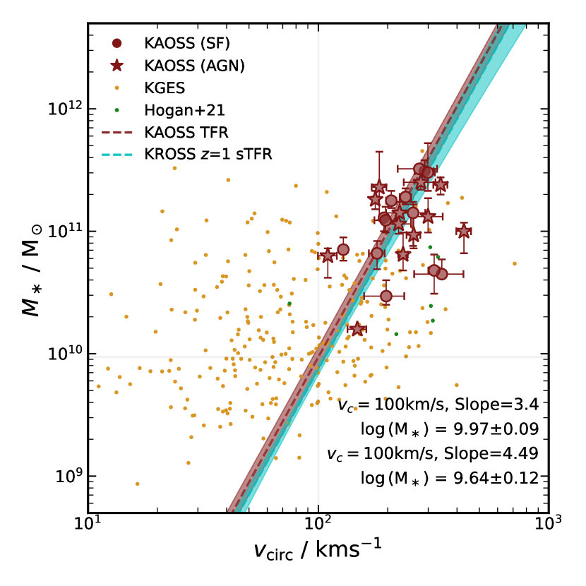
Figure 9: Stellar Tully-Fisher relation (sTFR): $v_{\rm circ}$ versus stellar mass for the KAOSS and KGES samples, along with $z$ $\sim$ 2.5 ULIRGs from Hogan et al. (2021). We fit for the normalisation of the Tully-Fisher relation, fixing the slope to be $a$ $=$ 3.4 (Tiley et al., 2019) and finding a best-fit normalisation of $\log_{10}(M_{\ast}/{\rm M}_{\odot})$ $=$ 9.97 $\pm$ 0.09 at $v_{\rm circ}$ $=$ 100 km s^-1, consistent with the value found by Tiley et al. (2019) for $z$ $=$ 0 SAMI galaxies, $\log_{10}(M_{\ast}/{\rm M}_{\odot})$ $=$ 9.87 $\pm$ 0.04.

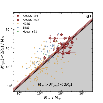
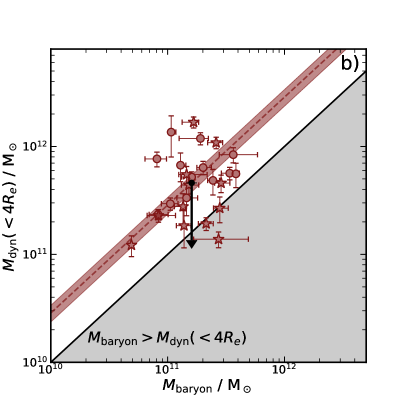
Figure 10: a) Dynamical masses of the resolved KAOSS sample, estimated from the H$\alpha$ kinematics within 2$R_{e}$, plotted against stellar masses. Plotted as a comparison are $z$ $\sim$ 1.5 KGES galaxies (Tiley et al., 2021), $z$ $\sim$ 2 SINS galaxies (Förster Schreiber et al., 2009) and $z$ $\sim$ 2.5 ULIRGs from Hogan et al. (2021). The black solid line indicates the 1:1 relation, and therefore points below this have stellar masses that are greater than their dynamical masses within 2$R_{e}$. b) The same as a) except here dynamical masses are estimated within 4$R_{e}$, and now plotted against baryonic mass, adding a gas component to the stellar mass by converting the magphys dust masses to gas masses using a gas-to-dust ratio of $\delta_{\rm gdr}$ $=$ 65 (Birkin et al., 2021). The black solid line is the same as in a). The vertical arrow indicates how far down the points would move if we were to adopt an aperture of 2$R_{e}$, in which case the baryonic masses are typically greater than the dynamical masses. We therefore suggest that much of the baryonic matter (in particular the cold molecular gas) is situated on radii larger than the stars in DSFGs.

4.6 Tully-Fisher relation

The Tully–Fisher relation (TFR; Tully & Fisher, 1977) connects the stellar or baryonic matter content of a galaxy to its dark matter. Our sample, which is one of the largest with estimates of kinematic information for DSFGs, allows us to probe the TFR relation for this massive galaxy population at $z$ $\sim$ 1.5–2.5. The TFR uses the rotational velocity of the interstellar medium as a proxy for the potential of the dark matter halo. This proxy is valid if the gas rotates in circular orbits, however as we have shown in §4.4 star-forming disc galaxies at high redshift are generally more turbulent systems than local galaxies (Wisnioski et al., 2015; Gillman et al., 2019), and these turbulent motions contribute to the dynamical support of the system (see §4.5), which reduces the necessary rotational support for a stable orbit. Before studying the TFR for KAOSS DSFGs we therefore estimate the circularised velocity $v_{\rm circ}$ according to:

$$v_{\rm circ}=\sqrt{\,v_{{\rm 2.2}R_{\rm d}}^{2}+2\sigma_{0}^{2}\left(\dfrac{R}{R_{\rm d}}\right)},$$ (4)

under the assumption of an exponential disc profile, where the pressure contribution to the rotational velocity is encapsulated by the $\sigma_{0}$ term, and we take $R$ $=$ 2.2 $R_{\rm d}$ (Burkert et al., 2010). For the KAOSS sample the median value of this quantity is $v_{\rm circ}$ $=$ 230 $\pm$ 20 km s^-1.

Fig. 9 shows the estimated circular velocity $v_{\rm circ}$ for the disc-like KAOSS resolved subset versus their stellar masses as estimated from magphys SED fitting (see §3.4). We also include similar measurements for KGES galaxies (Tiley et al., 2021) and Herschel-selected $z$ $\sim$ 2.5 ULIRGs from Hogan et al. (2021). In order to quantify the TFR for our $z$ $\sim$ 2 sample, and to test for any evolution against samples at lower redshifts, we fit to our data points the model $\log_{10}(v_{\rm circ})$ $=$ $a\log_{10}(M_{\ast})+b$ where $a$ and $b$ are constant parameters, using an orthogonal distance regression (ODR) method that takes both the errors in $M_{\ast}$ and $v_{\rm circ}$ into account.

Following Tiley et al. (2019) we measure the value of $\log_{10}(M_{\ast})$ at $v_{\rm circ}$ $=$ 100 km s^-1 and find $\log_{10}\left(M_{\ast}/{\rm M}_{\odot}\right)_{v_{2.2}=100}$ $=$ 9.97 $\pm$ 0.09 from the fit to our data. This is not systematically higher than the values measured by Tiley et al. (2019) for both the $z$ $\sim$ 1 KROSS (9.89 $\pm$ 0.04) and $z$ $\sim$ 0 SAMI (9.87 $\pm$ 0.04) samples, indicating no evolution in the sTFR between $z$ $\sim$ 2 and $z$ $\sim$ 0. In comparison with other studies, Bell & de Jong (2001) find $\log_{10}(M_{\ast})$ $=$ 9.5 at $v_{\rm max}$ $=$ 100 km s^-1 at $z$ $=$ 0, and Conselice et al. (2005) find corresponding values of 9.43 $\pm$ 0.12 and 9.39 $\pm$ 0.13 and $z$ $<$ 0.7 and $z$ $>$ 0.7, respectively. Both of the above are derived for a slope of 4.49. If we fix our slope to this value, we derive $\log_{10}(M_{\ast})$ $=$ 9.64 $\pm$ 0.12 at $v_{\rm max}$ $=$ 100 km s^-1 (this is noted in the legend of Fig. 9, but the fit itself is not shown). As with our comparison to the Tiley et al. (2019) samples, we do not see significant evidence for a change in the normalisation of the sTFR between $z$ $\sim$ 2 and the present day. This would suggest that in disc-like galaxies the rate of accretion of baryonic mass and dark matter is similar between $z$ $\sim$ 2 and $z$ $\sim$ 0.

4.7 Dynamical masses

The dynamical mass, i.e. the total matter content contributing to the motions of the galaxy, is another important quantity that is not yet well-measured for many DSFGs is the dynamical mass, and can be estimated using the kinematic information from our sample. We estimate dynamical masses within twice the effective radius, 2$R_{\rm e}$ (which is typically $\sim$ 7 kpc) for our sample according to:

$$M_{\rm dyn}(<2R_{\rm e})=\dfrac{2R_{\rm e}v_{\rm circ}^{2}}{G}$$ (5)

following Burkert et al. (2010), with $R$ $=$ 2$R_{\rm e}$. In Fig. 11 we show the dynamical mass estimates for our sample plotted against their stellar masses. Dynamical and baryonic masses are tabulated in the online supplementary table.

For sources in the KAOSS disc-like sample the median dynamical mass is $M_{\rm dyn}$ $=$ (1.6 $\pm$ 0.3) $\times$ 10¹¹ M_⊙, with a median $M_{\ast}$/$M_{\rm dyn}$ ratio of 0.94 $\pm$ 0.15, respectively. Therefore our sources are consistent with having no dark matter within a central radius of $R$ $\sim$ 7 kpc. Some authors have suggested that star-forming galaxies at high redshift are baryon dominated on scales of the disc (e.g. Genzel et al., 2017; Lang et al., 2017).

We therefore also consider the relation between dynamical mass and baryonic mass, shown in Fig. 10. Baryonic masses are derived according to:

$$M_{\rm baryon}=M_{\ast}+\delta_{\rm gdr}M_{\rm dust},$$ (6)

where $\delta_{\rm gdr}$ is the gas-to-dust ratio for which we adopt a value of 65, using the fit of Birkin et al. (2021) at $z$ $\sim$ 2. Contrary to the left panel of Fig. 10, we estimate dynamical masses within 4$R_{e}$, rather than 2$R_{e}$. From previous studies we expect $\sim$ 14 kpc to encompass the majority of the molecular gas (e.g. Ivison et al., 2011), which is approximately the median 4$R_{e}$ of our sample. We demonstrate by the downwards arrow where the points would lie if we had adopted an aperture of 2$R_{e}$ for the dynamical mass calculation. Although it is unclear how extended the cold molecular gas and dark matter is, Fig. 10 suggests that much of it is situated beyond the stellar matter in DSFGs, and this is supported by our median $M_{\rm baryon}$/$M_{\rm dyn}$ ratio of 0.36 $\pm$ 0.04, within 4$R_{e}$.

4.8 Descendants of DSFGs

It has been suggested that DSFGs are connected with the progenitors of local massive and compact early-type galaxies (e.g. Lilly et al., 1999; Simpson et al., 2014; Toft et al., 2014) in an evolutionary scenario involving obscured and unobscured QSO phases (e.g. Sanders et al., 1988; Blain et al., 2002; Swinbank et al., 2006; Hopkins et al., 2008). Several authors have provided evidence supporting this claim, such as Simpson et al. (2014) who showed that $z$ $\sim$ 0 DSFG descendants would have comparable stellar masses to massive early types (see also Dudzevičiūtė et al. 2020), and Hodge et al. (2016) found that ALESS DSFGs have gas surface densities and implied effective radii that are consistent with the most massive compact early-types. In Birkin et al. (2021) we compared CO-detected DSFGs with a sample of local early types in the Coma cluster (Shetty et al., 2020) in the $M_{\rm baryon}$–$\sigma$ and Age–$\sigma$ plane, finding the two populations to be consistent. However, the $\sigma$ values used in that work were estimated from CO linewidths without inclination corrections.

Our spatially resolved KMOS observations of DSFGs have provided inclination-corrected rotational and circularised velocities (see §4.1), from which we estimate $\sigma_{\rm eff}$ as (Binney & Tremaine, 2008):

$$\sigma_{\rm eff}=\dfrac{v_{\rm circ}}{\sqrt{2}},$$ (7)

to provide a more robust metric for comparing with the low-redshift sample. these values are presented in the online supplementary table. Fig. 11 shows $\sigma_{\rm eff}$ plotted against $M_{\rm baryon}$ for the KAOSS resolved subset, along with the CO-detected sources from Birkin et al. (2021) and local early-type galaxies from Shetty et al. (2020). We divide our sample into two bins in $M_{\rm baryon}$ and plot the median $\sigma_{\rm eff}$ with bootstrap uncertainties in these two bins, which are consistent with those of the CO sample, along with the early types, within their uncertainties. We see greater scatter among the KAOSS resolved sample compared to the early types, however, this appears to be driven by AGN-hosting DSFGs. We conclude from Fig. 11 that our spatially resolved KMOS observations support the suggestion that $z$ $\sim$ 2 DSFGs are consistent with them being the progenitors of massive and compact local early-type galaxies.

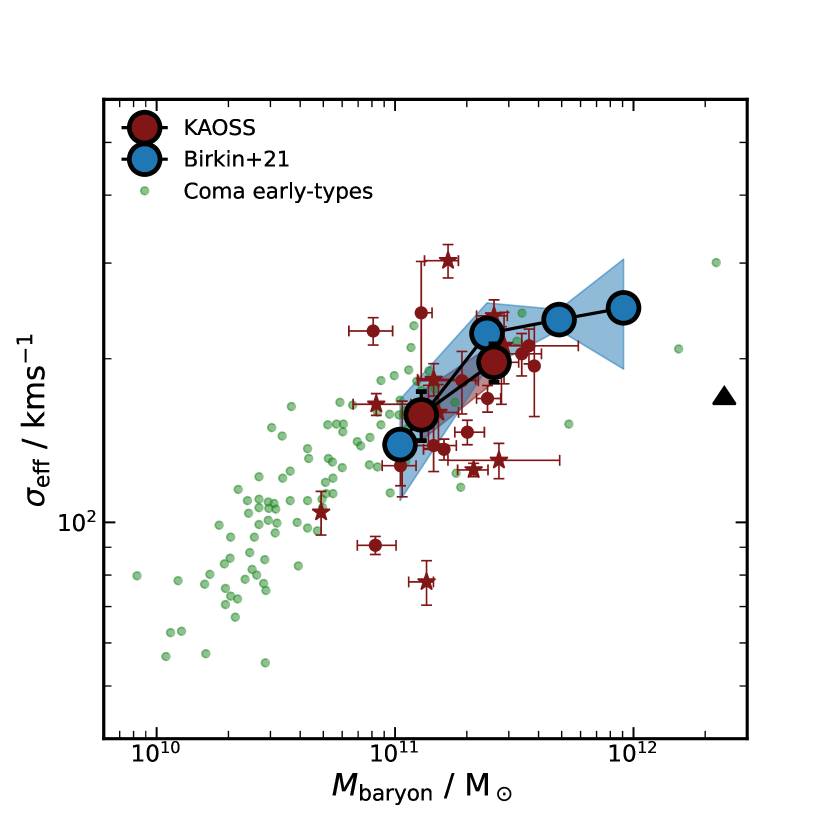
Figure 11: $M_{\rm baryon}$–$\sigma$ relation for KAOSS DSFGs and CO-detected DSFGs from Birkin et al. (2021), and early-type galaxies from the Coma cluster (Shetty et al., 2020). For KAOSS sources $M_{\rm baryon}$ is the sum of the magphys-derived stellar and cold gas masses (see §4.7). Our sample appears to have comparable estimated velocity dispersions with the early types, suggesting that they are plausibly connected with the descendant population of such sources.

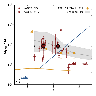
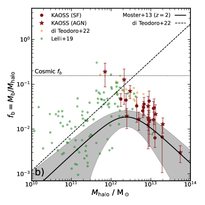
Figure 12: a) Halo mass versus redshift for the resolved KAOSS DSFGs, along with AS2UDS SMGs with halo masses estimated by Stach et al. (2021) based on a clustering analysis. The Dekel & Birnboim (2006) model suggests that the majority of our galaxies would reside in halos that experience shock heating. b) Stellar-to-halo mass versus halo mass for KAOSS DSFGs, along with local spiral galaxies compiled from Di Teodoro et al. (2022). We overlay the relation found by Moster et al. (2013) for $z$ $=$ 2 galaxies using abundance matching and its 1$\sigma$ deviation. The Moster et al. (2013) relation displays a break at $M_{\rm halo}$ $\sim$ 2 $\times$ 10¹² M_⊙, above which the majority of KAOSS DSFGs are consistent within its 1$\sigma$ deviation. However, three halos with masses below this threshold display much higher stellar-to-halo masses than expected by this relation. Notably, all three halos hosts DSFGs that we have classified as AGN hosts.

4.9 Stellar-to-halo mass ratio

Finally, motivated by the apparent lack of evolution of the stellar Tully-Fisher relation in §4.6, we turn to studying the stellar-to-halo mass relation (SHMR), which indicates how the stellar and dark matter halo grow in relation to one another. We parameterise this relation as $f_{M}$ $=$ $M_{\ast}$/$M_{\rm halo}$, and its variation with halo mass. The SHMR generally shows an increase in $f_{M}$ with stellar (or halo) mass, with a break seen at around $M_{\ast}$ $\sim$ 5 $\times$ 10¹⁰ M_⊙, or $M_{\rm halo}$ $\sim$ 10¹² M_⊙ which is interpreted as strong AGN feedback and mergers in galaxies with masses above the break (e.g Di Teodoro et al., 2022). This in turn prevents the further assembly of stellar mass, leading to a decreased $f_{M}$. It has recently been suggested by Posti & Fall (2021) that late-type galaxies do not follow this relation however, with AGN feedback in discs not strong enough to produce the break. This has been corroborated by hydrodynamical cosmological simulations (e.g. Correa & Schaye, 2020; Rodriguez-Gomez et al., 2022).

Several techniques have been employed in measuring the SHMR from observations, including galaxy clustering (Tinker et al., 2017; Stach et al., 2021), abundance matching (Behroozi et al., 2013; Moster et al., 2013) and kinematic modelling (Di Teodoro et al., 2022). To estimate masses for the halos in which the KAOSS DSFGs reside we compare our kinematic measurements with simulated star-forming galaxies in the Evolution and Assembly of GaLaxies and their Environments (EAGLE) simulation (Schaye et al., 2015). Specifically, we relate the stellar velocity dispersions $\sigma_{*}$ to our measured rotational velocities. We select EAGLE galaxies with SFR $>$ 10 M_⊙yr^-1 and $z$ $=$ 1.5–2.5 and remove satellite galaxies (we expect submillimetre-bright DSFGs to be central galaxies due to their high SFRs), and fit the relation between halo mass, $M_{\rm halo}$, and stellar velocity dispersion, determining the following calibration:

$$\log(M_{\rm halo}) =(3.32\pm 0.03)\log(\sigma_{*})+(5.17\pm 0.07),$$ (8)

from 2995 galaxies at $z\sim$ 1.5–2.5. We then adopt $v_{\rm circ}=$ 1.33 $\sigma_{*}$ following Serra et al. (2016), to relate the stellar velocity dispersion to $v_{\rm circ}$. We note that this relation was derived using Hi velocities measured at 6 $R_{e}$ in early-type galaxies, making this a crude approximation. In this analysis we do not expect this to be a dominant source of uncertainty, and hence to significantly affect our conclusions.

Halo masses for the DSFGs are tabulated in the online supplementary table. The disc-like sample has a median halo mass of $M_{\rm halo}$ $=$ (8.6 $\pm$ 1.6) $\times$ 10¹² M_⊙, and we show the individual halo masses as a function of redshift in Fig. 12, in which we indicate boundaries dividing the parameter space into the regions labelled “cold”, where galaxies can be fed by cold streams, “hot” where shock heating suppresses star formation and “cold in hot”, where cold streams can still feed the galaxy despite shock heating, based on the Dekel & Birnboim (2006) model of the thermal properties of gas flows onto galaxies. Most of the KAOSS DSFGs have estimated halo masses which suggest that they experience shock heating, the cause of which may be AGN feedback, a two-phase IGM, dynamical friction feedback, or a combination of the above (Dekel & Birnboim, 2006).

In Fig. 12 we also include halo masses estimated by Stach et al. (2021) for AS2UDS SMGs, using a clustering analysis, with which we find our binned data to be consistent with the 1$\sigma$ uncertainties, where the redshifts overlap. Additionally, both sets of data are consistent with the EAGLE prediction for submillimetre-bright galaxies (McAlpine et al., 2019). Our conclusion is therefore that KAOSS DSFGs reside in very massive ($\sim$ 10¹³ M_⊙) halos that are likely to contain large amounts of hot gas. At $z$ $\sim$ 2 the implied halo masses suggest that star formation can still be fed by cold streams (Dekel & Birnboim, 2006), whereas the lower-redshift sources lie in the region of the parameter space where shock heating would prevent this. Consequently, in such halos, another triggering mechanism may be needed to induce high SFRs, e.g. mergers and interactions (e.g. Alaghband-Zadeh et al., 2012; Chen et al., 2017).

Using the derived halo masses, along with stellar masses from magphys SED fitting, we proceed to test the SHMR for DSFGs, shown in Fig. 12. We compare with local spiral galaxies from Lelli et al. (2019) and Di Teodoro et al. (2022), and indicate the cosmic baryon fraction, $f_{b}$. All but one of our DSFGs are consistent with being below this boundary, with the only outlier being AS2COS0083.1, as a result of its unusually low rotational velocity ($v_{\rm rot}$ $=$ 29 $\pm$ 2 km s^-1). The majority of our sample are consistent with the relation derived by Moster et al. (2013), rather than the fit obtained by Di Teodoro et al. (2022) for spiral galaxies. This implies that our sources are experiencing strong feedback processes which are inhibiting stellar mass growth in halos with $M_{\rm halo}$ $>$ 10¹² M_⊙.

5 Conclusions

In this paper we have presented results from a subset of sources in the ongoing KMOS+ALMA Observations of Submillimetre Sources (KAOSS) Large Programme. We have measured H$\alpha$ velocity fields and extracted rotation curves for 31 DSFGs in the COSMOS, UDS and GOODS-S fields, allowing us to derive rotational velocities and dynamical masses, along with $v_{\rm rot}/\sigma_{0}$ ratios, to test the level of rotational support in the DSFG population. Our main results are as follows:

• We measure robust rotational velocities for a subsample of 25 out of the 31 resolved KAOSS sources from Freeman disc model fitting, finding a median inclination-corrected velocity at 2.2 times the disc radius of $v_{\rm rot}$ $=$ 190 $\pm$ 30 km s^-1. Therefore, 20 $\pm$ 8 per cent of the DSFGs are not well described by disc-like kinematics, and we make the assumption that these sources are pressure supported.

• We measure observed velocity dispersions, and by applying the beam-smearing corrections from Johnson et al. (2018), we derive intrinsic velocity dispersions, $\sigma_{0}$. The KAOSS resolved sample has a median $\sigma_{0}$ $=$ 87 $\pm$ 5 km s^-1, significantly higher than the samples of less actively star-forming galaxies with which we compare. This indicates high levels of turbulence in DSFGs.

• The median ratio of rotational velocity to intrinsic velocity dispersion is $v_{\rm rot}/\sigma_{0}$ $=$ 2.2 $\pm$ 0.5. We use this information with the above conclusions to suggest that KAOSS DSFGs are highly turbulent star-forming galaxies, which can be either rotationally supported or pressure supported.

• Our sources follow a trend between stellar mass $M_{\ast}$ and rotational velocity $v_{\rm rot}$ (the stellar Tully-Fisher relation), and we find a best-fit zeropoint at $v_{\rm rot}$ $=$ 100 km s^-1 of $\log_{10}(M_{\ast}/{\rm M}_{\odot})$ $=$ 9.97 $\pm$ 0.09, at a fixed slope of 3.4, which is consistent with the normalisation measured by Tiley et al. (2019) for $z$ $=$ 0 SAMI galaxies, $\log_{10}(M_{\ast}/{\rm M}_{\odot})$ $=$ 9.87 $\pm$ 0.04, at the same velocity. This suggests that dark matter and stellar mass growth are closely linked between $z$ $\sim$ 2 and the present day.

• The KAOSS DSFGs have a median dynamical mass within 2$R_{\rm e}$ ($\sim$ 7 kpc) of $M_{\rm dyn}$ $=$ (1.6 $\pm$ 0.3) $\times$ 10¹¹ M_⊙ and a median stellar-to-dynamical mass ratio of $M_{\ast}$/$M_{\rm dyn}$ $=$ 0.94 $\pm$ 0.15. Motivated by previous studies of the molecular gas in DSFGs, we derive baryonic mass within a radius of 4$R_{\rm e}$ ($\sim$ 7 kpc), finding a median baryonic-to-dynamical mass ratio of $M_{\rm bar}$/$M_{\rm dyn}$ $=$ 0.36 $\pm$ 0.04. We suggest that the majority of the baryonic matter in $z$ $\sim$ 2 DSFGs is situated beyond the extent of the stellar emission.

• Using the inclination-corrected velocity dispersions we estimate effective stellar velocity dispersions for the KAOSS DSFGs, finding them to be consistent with early-type galaxies in the Coma cluster, and therefore potential progenitors of such sources.

• The position of the KAOSS DSFGs in the stellar-to-halo mass relation indicate that most are experiencing strong feedback and/or shock heating leading to a decline in stellar mass in halos with masses above $\sim$ 10¹² M_⊙.

The current resolved KAOSS sample has doubled the sample size of DSFGs with spatially resolved kinematics. With the expected completion of the survey this year, this sample should approximately double in size, giving us the ability to draw more statistical conclusions about the nature of the population. Current and upcoming instrumentation will enable further improvements. For example, the Enhanced Resolution Imager and Spectrograph (ERIS) on the VLT will enable adaptive-optics assisted IFU observations, providing kinematics via the H$\alpha$ emission line on $\sim$ kpc scales. Similarly, with the NIRSpec instrument on the recently launched JWST we will be able to detect the H$\alpha$ line out to higher redshifts, and in IFU mode, to resolve DSFG kinematics out to higher redshifts, and at a much higher resolution than that of our KAOSS data. This will allow us to search for multiple components which would provide direct evidence of ongoing mergers in DSFGs.

Data availability

The data used in this paper are available through the ESO data archive, although some are currently still subject to a proprietary period of one year. Reduced data products can be shared upon publication by reasonable request to the author.

Appendix A Rotation curves

Fig. 13 show the H$\alpha$ rotation curves of the resolved KAOSS sources along with the derived velocity maps. These figures are discussed in more detail in §4.1.

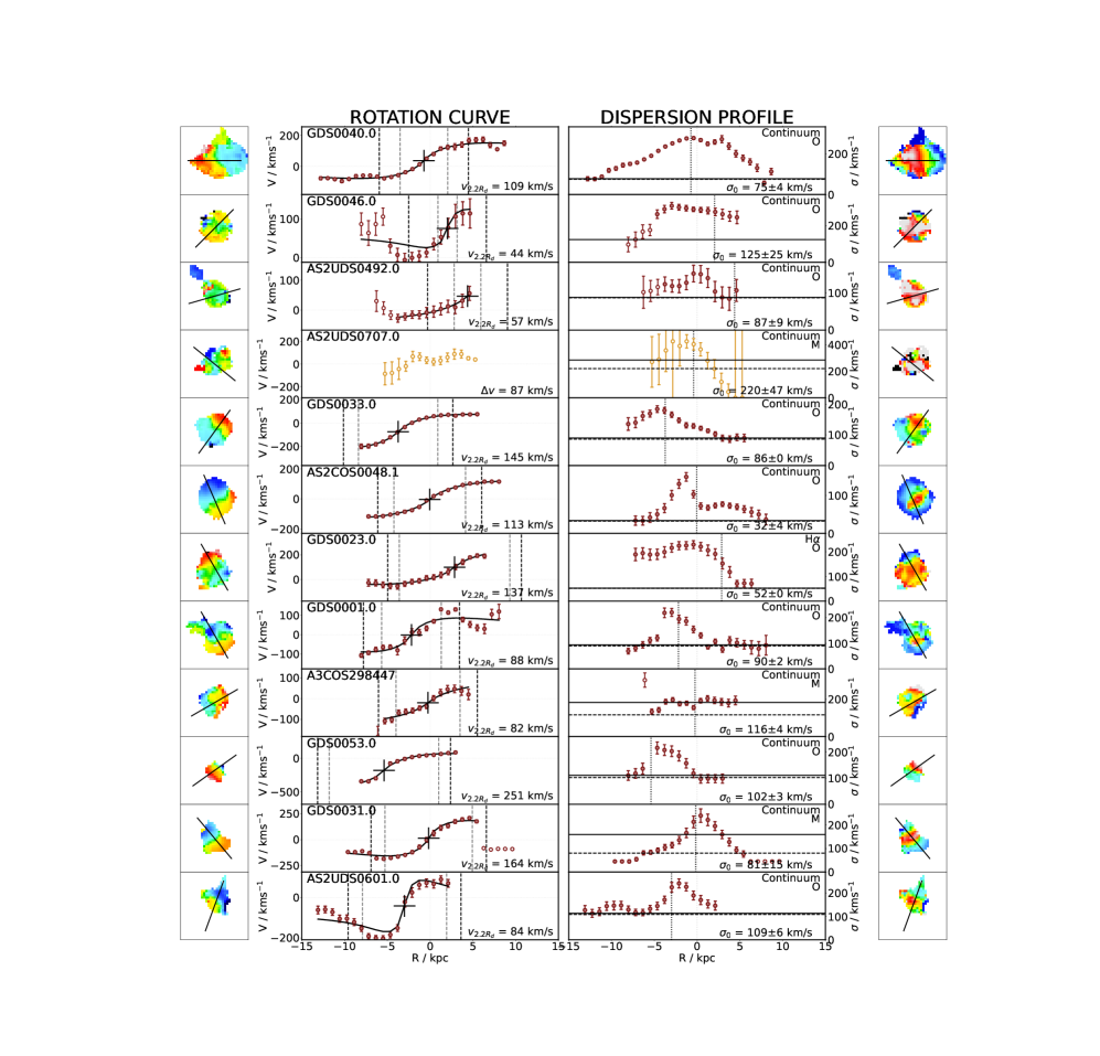
Figure 13: H$\alpha$ rotation curves (left) and velocity dispersion profiles (right) for the resolved KAOSS sample. Sources are ordered by the S/N of the H$\alpha$ emission line as in Fig. 2. The solid black lines indicate Freeman disc model fits to the data, the vertical dashed lines indicate $\pm$ 2.2 times the disc radius (thin) and $\pm$ 2.2 times the disc radius convolved with $\sigma_{\rm PSF}$ (thick), the latter at which we measure the rotation velocity, and the cross indicates the original source centroid. Points that are plotted as open circles are masked in the fitting procedure. For the dispersion profiles we indicate the observed velocity dispersion, $\sigma_{\rm obs}$ (horizontal black solid line), along with the method used to measure it (top right), and the beam smearing-corrected intrinsic velocity dispersion (horizontal black dashed line). We also indicate the method used to centre the velocity field in the top right corner of the dispersion profile panels.

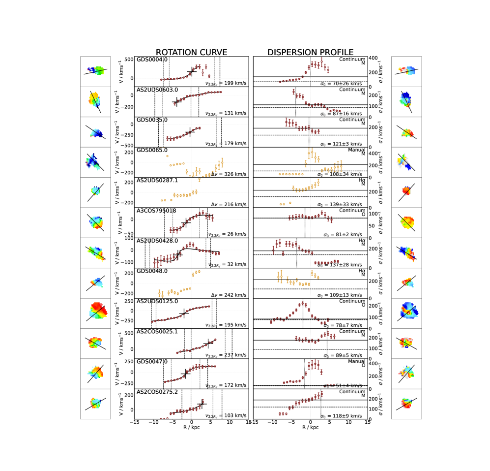
Figure A1 (Cont.):

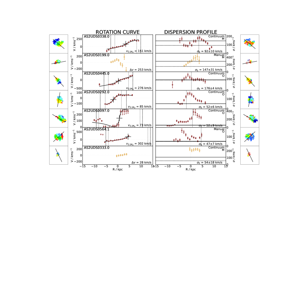
Figure A1 (Cont.):

Supporting information

Supplementary data are available at MNRAS online. We include a table of the properties used in this paper, with a README file describing each property. We also include a figure showing magphys SED fits to the photometry of the KAOSS resolved sample.

References

- Alaghband-Zadeh et al. (2012) Alaghband-Zadeh S., et al., 2012, MNRAS, 424, 2232
- Allen et al. (2008) Allen M. G., Groves B. A., Dopita M. A., Sutherland R. S., Kewley L. J., 2008, ApJS, 178, 20
- Behroozi et al. (2013) Behroozi P. S., Wechsler R. H., Conroy C., 2013, ApJ, 770, 57
- Bell & de Jong (2001) Bell E. F., de Jong R. S., 2001, ApJ, 550, 212
- Bellocchi et al. (2016) Bellocchi E., Arribas S., Colina L., 2016, A&A, 591, A85
- Binney & Tremaine (2008) Binney J., Tremaine S., 2008, Galactic Dynamics: Second Edition
- Birkin (2022) Birkin J. E., 2022, PhD thesis, Durham University, UK
- Birkin et al. (2021) Birkin J. E., et al., 2021, MNRAS, 501, 3926
- Blain et al. (2002) Blain A. W., Smail I., Ivison R. J., Kneib J. P., Frayer D. T., 2002, Phys. Rep., 369, 111
- Bothwell et al. (2013) Bothwell M. S., et al., 2013, MNRAS, 429, 3047
- Brinchmann et al. (2004) Brinchmann J., Charlot S., White S. D. M., Tremonti C., Kauffmann G., Heckman T., Brinkmann J., 2004, MNRAS, 351, 1151
- Bundy et al. (2015) Bundy K., et al., 2015, ApJ, 798, 7
- Burkert et al. (2010) Burkert A., et al., 2010, ApJ, 725, 2324
- Chen et al. (2017) Chen C.-C., et al., 2017, ApJ, 846, 108
- Civano et al. (2016) Civano F., et al., 2016, ApJ, 819, 62
- Conselice et al. (2005) Conselice C. J., Bundy K., Ellis R. S., Brichmann J., Vogt N. P., Phillips A. C., 2005, ApJ, 628, 160
- Correa & Schaye (2020) Correa C. A., Schaye J., 2020, MNRAS, 499, 3578
- Cowie et al. (2018) Cowie L. L., González-López J., Barger A. J., Bauer F. E., Hsu L. Y., Wang W. H., 2018, ApJ, 865, 106
- Cresci et al. (2009) Cresci G., et al., 2009, ApJ, 697, 115
- Croom et al. (2012) Croom S. M., et al., 2012, MNRAS, 421, 872
- Dekel & Birnboim (2006) Dekel A., Birnboim Y., 2006, MNRAS, 368, 2
- Di Teodoro et al. (2022) Di Teodoro E. M., et al., 2022, arXiv e-prints, p. arXiv:2207.02906
- Donley et al. (2012) Donley J. L., et al., 2012, ApJ, 748, 142
- Dudzevičiūtė et al. (2020) Dudzevičiūtė U., et al., 2020, MNRAS, 494, 3828
- ESO CPL Development Team (2015) ESO CPL Development Team 2015, EsoRex: ESO Recipe Execution Tool (ascl:1504.003)
- Elbaz et al. (2007) Elbaz D., et al., 2007, A&A, 468, 33
- Elbaz et al. (2011) Elbaz D., et al., 2011, A&A, 533, A119
- Fontana et al. (2014) Fontana A., et al., 2014, A&A, 570, A11
- Förster Schreiber et al. (2009) Förster Schreiber N. M., et al., 2009, ApJ, 706, 1364
- Franco et al. (2018) Franco M., et al., 2018, A&A, 620, A152
- Freeman (1970) Freeman K. C., 1970, ApJ, 160, 811
- Geach et al. (2017) Geach J. E., et al., 2017, MNRAS, 465, 1789
- Genzel et al. (2008) Genzel R., et al., 2008, ApJ, 687, 59
- Genzel et al. (2014) Genzel R., et al., 2014, ApJ, 796, 7
- Genzel et al. (2017) Genzel R., et al., 2017, Nature, 543, 397
- Giavalisco et al. (2004) Giavalisco M., et al., 2004, ApJ, 600, L93
- Gillman et al. (2019) Gillman S., et al., 2019, MNRAS, 486, 175
- Gillman et al. (2020) Gillman S., et al., 2020, MNRAS, 492, 1492
- Gnerucci et al. (2011) Gnerucci A., et al., 2011, A&A, 528, A88
- Gullberg et al. (2019) Gullberg B., et al., 2019, MNRAS, 490, 4956
- Guo et al. (2013) Guo Y., et al., 2013, ApJS, 207, 24
- Harrison et al. (2017) Harrison C. M., et al., 2017, MNRAS, 467, 1965
- Hodge et al. (2013) Hodge J. A., et al., 2013, ApJ, 768, 91
- Hodge et al. (2016) Hodge J. A., et al., 2016, ApJ, 833, 103
- Hogan et al. (2021) Hogan L., Rigopoulou D., Magdis G. E., Pereira-Santaella M., García-Bernete I., Thatte N., Grisdale K., Huang J. S., 2021, MNRAS, 503, 5329
- Hopkins et al. (2008) Hopkins P. F., Hernquist L., Cox T. J., Kereš D., 2008, ApJS, 175, 356
- Ivison et al. (2011) Ivison R. J., Papadopoulos P. P., Smail I., Greve T. R., Thomson A. P., Xilouris E. M., Chapman S. C., 2011, MNRAS, 412, 1913
- Jin et al. (2018) Jin S., et al., 2018, ApJ, 864, 56
- Johnson et al. (2018) Johnson H. L., et al., 2018, MNRAS, 474, 5076
- Kassin et al. (2007) Kassin S. A., et al., 2007, ApJ, 660, L35
- Kereš et al. (2005) Kereš D., Katz N., Weinberg D. H., Davé R., 2005, MNRAS, 363, 2
- Kewley & Ellison (2008) Kewley L. J., Ellison S. L., 2008, ApJ, 681, 1183
- Kim et al. (2011) Kim M., Dunlop J. S., Lonsdale C. J., Farrah D., Lacy M., Sun M., SpUDS Team 2011, in American Astronomical Society Meeting Abstracts #217. p. 335.51
- Kocevski et al. (2018) Kocevski D. D., et al., 2018, ApJS, 236, 48
- Lagattuta et al. (2013) Lagattuta D. J., Mould J. R., Staveley-Smith L., Hong T., Springob C. M., Masters K. L., Koribalski B. S., Jones D. H., 2013, ApJ, 771, 88
- Lagos et al. (2020) Lagos C. d. P., da Cunha E., Robotham A. S. G., Obreschkow D., Valentino F., Fujimoto S., Magdis G. E., Tobar R., 2020, arXiv e-prints, p. arXiv:2007.09853
- Laigle et al. (2016) Laigle C., et al., 2016, ApJS, 224, 24
- Lang et al. (2017) Lang P., et al., 2017, ApJ, 840, 92
- Lapi et al. (2018) Lapi A., et al., 2018, ApJ, 857, 22
- Law et al. (2009) Law D. R., Steidel C. C., Erb D. K., Larkin J. E., Pettini M., Shapley A. E., Wright S. A., 2009, ApJ, 697, 2057
- Lawrence et al. (2007) Lawrence A., et al., 2007, MNRAS, 379, 1599
- Lelli et al. (2019) Lelli F., McGaugh S. S., Schombert J. M., Desmond H., Katz H., 2019, MNRAS, 484, 3267
- Lilly et al. (1999) Lilly S. J., Eales S. A., Gear W. K. P., Hammer F., Le Fèvre O., Crampton D., Bond J. R., Dunne L., 1999, ApJ, 518, 641
- Liu et al. (2019) Liu D., et al., 2019, ApJS, 244, 40
- Luo et al. (2017) Luo B., et al., 2017, ApJS, 228, 2
- Magnelli et al. (2012) Magnelli B., et al., 2012, A&A, 539, A155
- Mancini et al. (2011) Mancini C., et al., 2011, ApJ, 743, 86
- McAlpine et al. (2019) McAlpine S., et al., 2019, MNRAS, 488, 2440
- McCracken et al. (2012) McCracken H. J., et al., 2012, A&A, 544, A156
- Menéndez-Delmestre et al. (2013) Menéndez-Delmestre K., Blain A. W., Swinbank M., Smail I., Ivison R. J., Chapman S. C., Gonçalves T. S., 2013, ApJ, 767, 151
- Miettinen et al. (2017) Miettinen O., et al., 2017, A&A, 606, A17
- Miller et al. (2013) Miller N. A., et al., 2013, ApJS, 205, 13
- Moster et al. (2013) Moster B. P., Naab T., White S. D. M., 2013, MNRAS, 428, 3121
- Narayanan et al. (2009) Narayanan D., Cox T. J., Hayward C. C., Younger J. D., Hernquist L., 2009, MNRAS, 400, 1919
- Narayanan et al. (2010) Narayanan D., Hayward C. C., Cox T. J., Hernquist L., Jonsson P., Younger J. D., Groves B., 2010, MNRAS, 401, 1613
- Narayanan et al. (2015) Narayanan D., et al., 2015, Nature, 525, 496
- Newman et al. (2013) Newman S. F., et al., 2013, ApJ, 767, 104
- Noeske et al. (2007) Noeske K. G., et al., 2007, ApJ, 660, L43
- Olivares et al. (2016) Olivares V., et al., 2016, ApJ, 827, 57
- Oliver et al. (2012) Oliver S. J., et al., 2012, MNRAS, 424, 1614
- Osterbrock & Ferland (2006) Osterbrock D. E., Ferland G. J., 2006, Astrophysics of gaseous nebulae and active galactic nuclei
- Peng et al. (2010) Peng C. Y., Ho L. C., Impey C. D., Rix H.-W., 2010, AJ, 139, 2097
- Posti & Fall (2021) Posti L., Fall S. M., 2021, A&A, 649, A119
- Rizzo et al. (2021) Rizzo F., Vegetti S., Fraternali F., Stacey H. R., Powell D., 2021, MNRAS, 507, 3952
- Rodriguez-Gomez et al. (2022) Rodriguez-Gomez V., et al., 2022, MNRAS, 512, 5978
- Sánchez et al. (2012) Sánchez S. F., et al., 2012, A&A, 538, A8
- Sanders et al. (1988) Sanders D. B., Soifer B. T., Elias J. H., Madore B. F., Matthews K., Neugebauer G., Scoville N. Z., 1988, ApJ, 325, 74
- Schaye et al. (2015) Schaye J., et al., 2015, MNRAS, 446, 521
- Schreiber et al. (2015) Schreiber C., et al., 2015, A&A, 575, A74
- Serra et al. (2016) Serra P., Oosterloo T., Cappellari M., den Heijer M., Józsa G. I. G., 2016, MNRAS, 460, 1382
- Sharples et al. (2013) Sharples R., et al., 2013, The Messenger, 151, 21
- Shetty et al. (2020) Shetty S., Cappellari M., McDermid R. M., Krajnović D., de Zeeuw P. T., Davies R. L., Kobayashi C., 2020, MNRAS, 494, 5619
- Shim et al. (2022) Shim H., et al., 2022, MNRAS,
- Simpson et al. (2013) Simpson C., Westoby P., Arumugam V., Ivison R., Hartley W., Almaini O., 2013, MNRAS, 433, 2647
- Simpson et al. (2014) Simpson J. M., et al., 2014, ApJ, 788, 125
- Simpson et al. (2019) Simpson J. M., et al., 2019, ApJ, 880, 43
- Simpson et al. (2020) Simpson J. M., et al., 2020, arXiv e-prints, p. arXiv:2003.05484
- Smolčić et al. (2017) Smolčić V., et al., 2017, A&A, 602, A1
- Soto et al. (2016) Soto K. T., Lilly S. J., Bacon R., Richard J., Conseil S., 2016, MNRAS, 458, 3210
- Speagle et al. (2014) Speagle J. S., Steinhardt C. L., Capak P. L., Silverman J. D., 2014, ApJS, 214, 15
- Stach et al. (2019) Stach S. M., et al., 2019, MNRAS, 487, 4648
- Stach et al. (2021) Stach S. M., et al., 2021, MNRAS, 504, 172
- Stott et al. (2016) Stott J. P., et al., 2016, MNRAS, 457, 1888
- Swinbank et al. (2006) Swinbank A. M., Chapman S. C., Smail I., Lindner C., Borys C., Blain A. W., Ivison R. J., Lewis G. F., 2006, MNRAS, 371, 465
- Swinbank et al. (2012) Swinbank A. M., Smail I., Sobral D., Theuns T., Best P. N., Geach J. E., 2012, ApJ, 760, 130
- Swinbank et al. (2014) Swinbank A. M., et al., 2014, MNRAS, 438, 1267
- Tacconi et al. (2006) Tacconi L. J., et al., 2006, ApJ, 640, 228
- Tacconi et al. (2020) Tacconi L. J., Genzel R., Sternberg A., 2020, ARA&A, 58, 157
- Tiley et al. (2019) Tiley A. L., et al., 2019, MNRAS, 482, 2166
- Tiley et al. (2021) Tiley A. L., et al., 2021, MNRAS, 506, 323
- Tinker et al. (2017) Tinker J. L., et al., 2017, ApJ, 839, 121
- Toft et al. (2014) Toft S., et al., 2014, ApJ, 782, 68
- Tully & Fisher (1977) Tully R. B., Fisher J. R., 1977, A&A, 54, 661
- Tully & Pierce (2000) Tully R. B., Pierce M. J., 2000, ApJ, 533, 744
- Turner et al. (2017) Turner O. J., et al., 2017, MNRAS, 471, 1280
- Übler et al. (2017) Übler H., et al., 2017, ApJ, 842, 121
- Weiner et al. (2006) Weiner B. J., et al., 2006, ApJ, 653, 1027
- Whitaker et al. (2012) Whitaker K. E., van Dokkum P. G., Brammer G., Franx M., 2012, ApJ, 754, L29
- Wisnioski et al. (2015) Wisnioski E., et al., 2015, ApJ, 799, 209
- Wisnioski et al. (2018) Wisnioski E., et al., 2018, ApJ, 855, 97
- Wisnioski et al. (2019) Wisnioski E., et al., 2019, ApJ, 886, 124
- da Cunha et al. (2015) da Cunha E., et al., 2015, ApJ, 806, 110