Topological Quantum Dimers Emerging from Kitaev Spin Liquid Bilayer:
Anyon Condensation Transition

Abstract

We present a bilayer spin model that illuminates the mechanism of topological anyon condensation transition. Our model harbors two distinct topological phases, Kitaev spin liquid bilayer state and resonating valence bond (RVB) state connected by a continuous transition. We show that the transition occurs by anyon condensation, and the hardcore dimer constraint of the RVB state plays a role of the order parameter. This model study offers an intuitive picture for anyon condensation transition, and is broadly applicable to generic tri-coordinated lattices preserving the emergence of the RVB state from the Kitaev bilayer.

Introduction. Anyons are exotic fractional particles emerging in many-body quantum entangled states such as quantum spin liquids (QSLs) Kitaev (2003, 2006); Savary and Balents (2016); Zhou et al. (2017); Knolle and Moessner (2019); Broholm et al. (2020); Wen (2004); Fradkin (2013); Sachdev (2023). Recently, various QSLs with anyon quasiparticles have been active subjects of research due to potential applications in quantum technology. Kitaev spin liquid states Kitaev (2003, 2006) and resonating valence bond states Rokhsar and Kivelson (1988); Moessner and Sondhi (2001); Misguich et al. (2002); Samajdar et al. (2021); Verresen et al. (2021); Verresen and Vishwanath (2022) are promising examples which have not only exact solutions but also available experimental platforms such as the quantum magnet $\alpha$-RuCl₃, quantum processor, and Rydberg atom arrays Kasahara et al. (2018); Takagi et al. (2019); Satzinger et al. (2021); Semeghini et al. (2021).

Anyon condensation is a theoretical mechanism that explains transitions between distinct topological phases supporting anyons Bais and Slingerland (2009); Burnell et al. (2011, 2012); Eliëns et al. (2014); Neupert et al. (2016); Schulz and Burnell (2016); Burnell (2018); Wang et al. (2021). In this mechanism, anyon condensation gives rise to the reconstruction of quantum entanglement and allowed anyon quasiparticles in the condensed phase. The mechanism provides global insights on how a variety of different topological phases can be connected. However, it has been elusive to confirm the mechanism in quantum spin systems because of the scarcity of appropriate microscopic models and the difficulty with defining an order parameter for anyon condensation in terms of spin operators.

In this letter, we introduce a bilayer spin model that enables to study an anyon condensation transition between different QSLs. The bilayer model has a Kitaev spin liquid (KSL) bilayer state and a resonating valence bond (RVB) state in different limits. The RVB state is induced by entangling the bilayer system in a certain way. The onset of the RVB state is characterized by the calculations of entanglement entropy, hardcore dimer constraint, and topological degeneracy via exact diagonalization.

We identify the nature of the transition between the QSLs by calculating an order parameter for anyon condensation. This work offers an intuitive picture about anyon condensation transition with a concrete microscopic model realizing ${\rm Ising}\times\overline{\rm Ising}$ and $\mathbb{Z}_{2}$ topological orders.

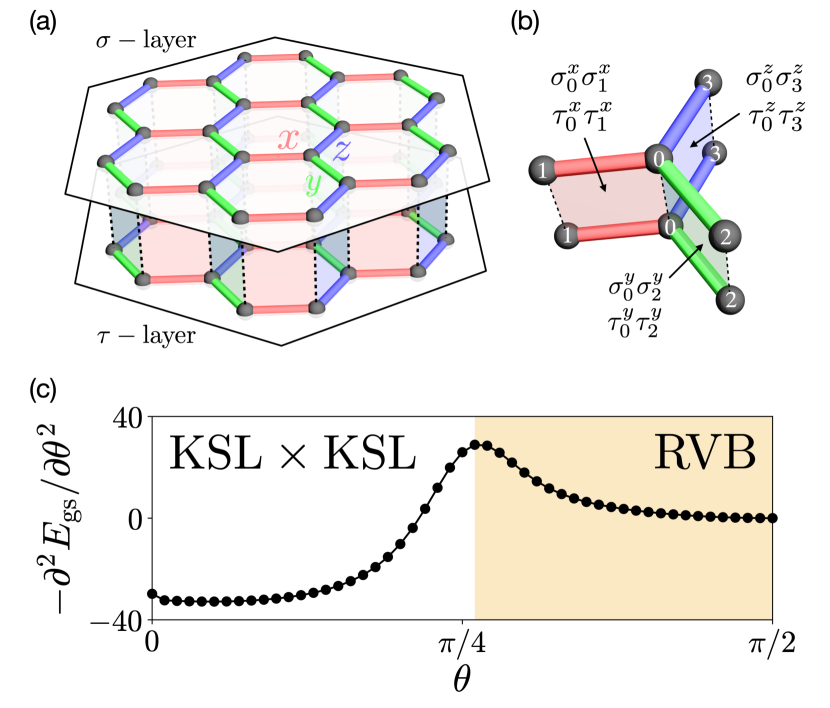
Figure 1: Bilayer model. (a) Honeycomb lattice bilayer with the AA stacking. $\sigma$ and $\tau$ spins reside on the upper and lower layers, and the $x,y,z$-bonds are denoted by different colors of red, green, blue. The figure depicts the $(24+24)$-site bilayer cluster used in our exact diagonalization. (b) Four-spin inter-layer interactions. (c) The phase diagram of the model. The KSL$\times$KSL and RVB states are connected by a second order continuous transition at $\theta_{c}\simeq 0.26\pi$; indicated by a small peak in the derivative of the ground state energy, $-\partial^{2}E_{\rm gs}/\partial\theta^{2}$.

Bilayer model. We place two copies of the Kitaev honeycomb model on a bilayer geometry of AA stacking [Fig. 1(a)]. Our model Hamiltonian consists of three parts:

$$H = K_{\sigma}\sum_{\langle jk\rangle_{\gamma}}^{\textup{upper~{}layer}}\sigma_{j}^{\gamma}\sigma_{k}^{\gamma}+K_{\tau}\sum_{\langle jk\rangle_{\gamma}}^{\textup{lower~{}layer}}\tau_{j}^{\gamma}\tau_{k}^{\gamma}$$ (1)

$$+ G\sum_{\langle jk\rangle_{\gamma}}^{\textup{inter-layer}}\sigma_{j}^{\gamma}\sigma_{k}^{\gamma}\tau_{j}^{\gamma}\tau_{k}^{\gamma},$$

where $\sigma^{\gamma}$ and $\tau^{\gamma}$ ($\gamma=x,y,z$) are Pauli spins on the upper and lower layers coupled by the bond-dependent Kitaev interactions ($K_{\sigma}$, $K_{\tau}$) Kitaev (2006) and also the inter-layer interactions ($G$). We label upper and lower layer spins with same site-indices ($j,k$), and the inter-layer interactions are nothing but the products of adjacent upper-layer and lower-layer Kitaev interactions, $\sigma_{j}^{\gamma}\sigma_{k}^{\gamma}\times\tau_{j}^{\gamma}\tau_{k}^{\gamma}$ [Fig. 1(b)]. The Hamiltonian commutes with the hexagon plaquette operators defined on the upper and lower layers,

$$\hat{W}_{p}=\sigma_{1}^{z}\sigma_{2}^{y}\sigma_{3}^{x}\sigma_{4}^{z}\sigma_{5}^{y}\sigma_{6}^{x}~{}~{}~{}~{}\&~{}~{}~{}~{}\hat{Z}_{p}=\tau_{1}^{z}\tau_{2}^{y}\tau_{3}^{x}\tau_{4}^{z}\tau_{5}^{y}\tau_{6}^{x},$$ (2)

i.e., $[H,\hat{W}_{p}]=[H,\hat{Z}_{p}]=[\hat{W}_{p},\hat{Z}_{p^{\prime}}]=0$; see Fig. 2(a) for the site convention within a hexagon plaquette $p$.

In this paper, we focus on the parameter region,

$$K_{\sigma}=-K_{\tau}=\cos\theta~{}~{}~{}\&~{}~{}~{}G=\sin\theta,$$ (3)

where $0\leq\theta\leq\pi/2$. We show two distinct quantum spin liquids: (i) KSL$\times$KSL bilayer product state in the weak coupling limit, $|K_{\sigma,\tau}|\gg G$ ($\theta\approx 0$), and (ii) RVB state in the strong coupling limit, $|K_{\sigma,\tau}|\ll G$ ($\theta\approx\pi/2$). General cases beyond Eq. (3) are discussed in Supplemental Material SM .

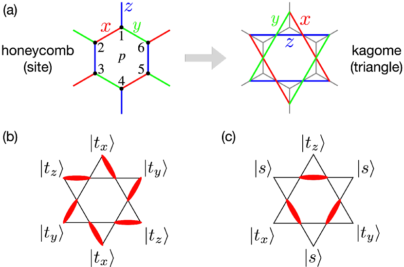
$\sigma^{z}\otimes\tau^{z}$ basis	$|\phi^{x},\phi^{y},\phi^{z}\rangle$ basis	Dimer rep.
$|s\rangle=\frac{1}{\sqrt{2}}(|\uparrow\downarrow\rangle-|\downarrow\uparrow\rangle)$	$|-1,-1,-1\rangle$
$|t_{x}\rangle=\frac{-1}{\sqrt{2}}(|\uparrow\uparrow\rangle-|\downarrow\downarrow\rangle)$	$|-1,+1,+1\rangle$
$|t_{y}\rangle=\frac{i}{\sqrt{2}}(|\uparrow\uparrow\rangle+|\downarrow\downarrow\rangle)$	$|+1,-1,+1\rangle$
$|t_{z}\rangle=\frac{1}{\sqrt{2}}(|\uparrow\downarrow\rangle+|\downarrow\uparrow\rangle)$	$|+1,+1,-1\rangle$

Figure 2: Dimer mapping to the dual kagome lattice. (a) Mapping from the honeycomb lattice to the kagome lattice. Different color lines denote the three bond characters, $x$(red), $y$(green), $z$(blue). The numbers ($1\sim 6$) indicate the site convention within a hexagon plaquette $p$. (b),(c) Illustrations of dimer states. The four local states $\{|s\rangle,|t_{x}\rangle,|t_{y}\rangle,|t_{z}\rangle\}$ and the dimer mapping are defined in the bottom table.

Dimer representation on a dual kagome lattice. We employ a dimer representation which helps to understand the strong coupling limit. The bilayer model can be regarded as a single layer honeycomb model with four states per site. Each site may have either spin-singlet state $|s\rangle$ or spin-triplet state $|t_{x,y,z}\rangle$ as shown in the table of Fig. 2.

We take a mapping from the honeycomb lattice to a dual kagome lattice. In Fig. 2(a), the dual kagome lattice is constructed by connecting the mid-points of the bonds of the honeycomb lattice. Sites of the honeycomb lattice are now replaced by triangles of the kagome lattice. Interestingly, the kagome lattice has three different bond directions, which are perpendicular to the $x,y,z$-bond directions of the honeycomb lattice. By using this property, we assign a bond character ($x,y,z$) to each bond of the kagome lattice [denoted by different colors in Fig. 2(a)]. In this mapping, the four local states $\{|s\rangle,|t_{x}\rangle,|t_{y}\rangle,|t_{z}\rangle\}$ on the honeycomb lattice are represented by four dimer states $\{|\parbox{11.38092pt}{\includegraphics[width=433.62pt]{./dimer-s.pdf}}\rangle,|\parbox{11.38092pt}{\includegraphics[width=433.62pt]{./dimer-tx.pdf}}\rangle,|\parbox{11.38092pt}{\includegraphics[width=433.62pt]{./dimer-ty.pdf}}\rangle,|\parbox{11.38092pt}{\includegraphics[width=433.62pt]{./dimer-tz.pdf}}\rangle\}$ on the dual kagome lattice. The $|s\rangle$ state is the no-dimer state at the corresponding local triangle of the kagome lattice while the $|t_{\gamma}\rangle$ state is the dimer state occupying the ${\gamma}$-bond of the local triangle. See Fig. 2(b),(c). This kind of mapping was introduced in a recent study of dimer model Verresen and Vishwanath (2022).

With the dimer mapping, spin operators take the following representations.

$$\sigma^{z} = |s\rangle\langle t_{z}|+|t_{z}\rangle\langle s|-i|t_{x}\rangle\langle t_{y}|+i|t_{y}\rangle\langle t_{x}|$$ (4)

$$= |\parbox{11.38092pt}{\includegraphics[width=433.62pt]{./dimer-s.pdf}}\rangle\langle\parbox{11.38092pt}{\includegraphics[width=433.62pt]{./dimer-tz.pdf}}|+|\parbox{11.38092pt}{\includegraphics[width=433.62pt]{./dimer-tz.pdf}}\rangle\langle\parbox{11.38092pt}{\includegraphics[width=433.62pt]{./dimer-s.pdf}}|-i|\parbox{11.38092pt}{\includegraphics[width=433.62pt]{./dimer-tx.pdf}}\rangle\langle\parbox{11.38092pt}{\includegraphics[width=433.62pt]{./dimer-ty.pdf}}|+i|\parbox{11.38092pt}{\includegraphics[width=433.62pt]{./dimer-ty.pdf}}\rangle\langle\parbox{11.38092pt}{\includegraphics[width=433.62pt]{./dimer-tx.pdf}}|.~{}~{}~{}~{}~{}$$

$$\tau^{z} = -|s\rangle\langle t_{z}|-|t_{z}\rangle\langle s|-i|t_{x}\rangle\langle t_{y}|+i|t_{y}\rangle\langle t_{x}|$$ (5)

$$= -|\parbox{11.38092pt}{\includegraphics[width=433.62pt]{./dimer-s.pdf}}\rangle\langle\parbox{11.38092pt}{\includegraphics[width=433.62pt]{./dimer-tz.pdf}}|-|\parbox{11.38092pt}{\includegraphics[width=433.62pt]{./dimer-tz.pdf}}\rangle\langle\parbox{11.38092pt}{\includegraphics[width=433.62pt]{./dimer-s.pdf}}|-i|\parbox{11.38092pt}{\includegraphics[width=433.62pt]{./dimer-tx.pdf}}\rangle\langle\parbox{11.38092pt}{\includegraphics[width=433.62pt]{./dimer-ty.pdf}}|+i|\parbox{11.38092pt}{\includegraphics[width=433.62pt]{./dimer-ty.pdf}}\rangle\langle\parbox{11.38092pt}{\includegraphics[width=433.62pt]{./dimer-tx.pdf}}|.~{}~{}~{}~{}~{}$$

Other spin operators are obtained by cyclic permutations of ($x,y,z$) in the above. In the dimer picture, $\sigma^{z}$ and $\tau^{z}$ do monomer pair-creation/annihilation or monomer hopping at the $z$-bond of the kagome lattice, and similarly for other spin operators.

Emergence of resonating valence bonds. The strong coupling limit of $H$ is investigated by a perturbation theory. In this case, the unperturbed Hamiltonian is the inter-layer interaction part:

$$H_{0}=G\sum_{\langle jk\rangle_{\gamma}}\phi_{j}^{\gamma}\phi_{k}^{\gamma}.$$ (6)

Here we employed the composite spin operator,

$$\phi_{j}^{\gamma}\equiv\sigma_{j}^{\gamma}\tau_{j}^{\gamma},$$ (7)

which is $\mathbb{Z}_{2}$-valued [$(\phi_{j}^{\gamma})^{2}=1$] and satisfies the relations, $[\phi_{j}^{\gamma},\phi_{k}^{\lambda}]=0$ & $\phi_{j}^{x}\phi_{j}^{y}\phi_{j}^{z}=-1$.

Remarkably, the four states $\{|s\rangle,|t_{x}\rangle,|t_{y}\rangle,|t_{z}\rangle\}$ are the eigenstates of the composite spin operators ($\phi^{x},\phi^{y},\phi^{z}$) as summarized in the table of Fig. 2. The composite spin operators take simple dimer representations, e.g.,

$$\phi^{z} = -|s\rangle\langle s|+|t_{x}\rangle\langle t_{x}|+|t_{y}\rangle\langle t_{y}|-|t_{z}\rangle\langle t_{z}|$$ (8)

$$= -|\parbox{11.38092pt}{\includegraphics[width=433.62pt]{./dimer-s.pdf}}\rangle\langle\parbox{11.38092pt}{\includegraphics[width=433.62pt]{./dimer-s.pdf}}|+|\parbox{11.38092pt}{\includegraphics[width=433.62pt]{./dimer-tx.pdf}}\rangle\langle\parbox{11.38092pt}{\includegraphics[width=433.62pt]{./dimer-tx.pdf}}|+|\parbox{11.38092pt}{\includegraphics[width=433.62pt]{./dimer-ty.pdf}}\rangle\langle\parbox{11.38092pt}{\includegraphics[width=433.62pt]{./dimer-ty.pdf}}|-|\parbox{11.38092pt}{\includegraphics[width=433.62pt]{./dimer-tz.pdf}}\rangle\langle\parbox{11.38092pt}{\includegraphics[width=433.62pt]{./dimer-tz.pdf}}|.~{}~{}~{}~{}~{}$$

Note that $-\phi^{z}$ measures the dimer parity across the $x,y$-bonds, and similarly for $-\phi^{x,y}$.

The unperturbed Hamiltonian $H_{0}$ is readily diagonalized in the dimer representation. We find that the ground state manifold of $H_{0}$ is extensively degenerate satisfying the condition,

$$\phi_{j}^{\gamma}\phi_{k}^{\gamma}=-1,$$ (9)

at every bond $\langle jk\rangle_{\gamma}$ of the honeycomb lattice. This condition implies the “hardcore dimer” constraint on the kagome lattice, i.e., each site of the kagome lattice is occupied by a single dimer. Specifically, the condition $\phi_{j}^{\gamma}\phi_{k}^{\gamma}=-1$ only allows the eight configurations,

$$\parbox{14.22636pt}{\includegraphics[width=433.62pt]{./hardcore-1.pdf}},~{}~{}~{}\parbox{14.22636pt}{\includegraphics[width=433.62pt]{./hardcore-2.pdf}},~{}~{}~{}\parbox{14.22636pt}{\includegraphics[width=433.62pt]{./hardcore-3.pdf}},~{}~{}~{}\parbox{14.22636pt}{\includegraphics[width=433.62pt]{./hardcore-4.pdf}},~{}~{}~{}\parbox{14.22636pt}{\includegraphics[width=433.62pt]{./hardcore-5.pdf}},~{}~{}~{}\parbox{14.22636pt}{\includegraphics[width=433.62pt]{./hardcore-6.pdf}},~{}~{}~{}\parbox{14.22636pt}{\includegraphics[width=433.62pt]{./hardcore-7.pdf}},~{}~{}~{}\parbox{14.22636pt}{\includegraphics[width=433.62pt]{./hardcore-8.pdf}},$$

in every adjacent two triangles. The central site is always occupied by a single dimer because the condition $\phi_{j}^{\gamma}\phi_{k}^{\gamma}=-1$ requires the odd dimer parity over the four bonds connected to the central site. Hence, the ground state manifold of $H_{0}$ consists of the dimer states that respect the hardcore dimer constraint. The ground state energy is $E_{0}=-\frac{3N}{2}|G|$, where $N$ is the number of sites of the honeycomb lattice, and the degeneracy is given by $2^{N/2-1}$ in periodic boundary condition.

The Kitaev terms in $H$ generate quantum dimer motions in the ground state manifold of $H_{0}$. By perturbative expansions within the manifold, we obtain the effective Hamiltonian,

$${\mathcal{H}_{\rm eff}(G\gg K)}=-\lambda\sum_{p}\hat{W}_{p},$$ (10)

where $\hat{W}_{p}$ is the hexagon plaquette operator in Eq. (2), and $\lambda\propto K_{\sigma}^{6}/G^{5}$ (Supplemental Material SM ). It is straightforward to find the ground state of $\mathcal{H}_{\rm eff}(G\gg K)$,

$$|\Psi\rangle=\mathcal{N}\prod_{p}\frac{1+\hat{W}_{p}}{2}|\Phi\rangle,$$ (11)

where $\mathcal{N}$ is a normalization factor and $|\Phi\rangle$ is an arbitrary state in the ground state manifold of $H_{0}$. This state is a massively quantum superposed state with the uniform zero-flux (${W}_{p}={Z}_{p}=+1$). It has the property, $\langle\sigma_{j}^{\gamma}\sigma_{k}^{\gamma}\rangle=\langle\tau_{j}^{\gamma}\tau_{k}^{\gamma}\rangle=0$, because the Kitaev terms violate the hardcore dimer constraint [Eq. (9)].

The ground state $|\Psi\rangle$ is nothing but a resonating valence bond state on the kagome lattice. To see this, one should understand the effects of $\hat{W}_{p}$ in the dimer language. Acting on hardcore dimer states, $\hat{W}_{p}$ gives rise to dimer resonance motions within the 12-site David star as follows.

$$\hat{W}_{p} = \sum_{\mathpzc{D}}f(\mathpzc{D})|\mathpzc{D}\rangle\langle\bar{\mathpzc{D}}|+{\rm H.c.}$$ (12)

$$= |\parbox{17.07182pt}{\includegraphics[width=433.62pt]{./hexagon.pdf}}\rangle\langle\parbox{17.07182pt}{\includegraphics[width=433.62pt]{./hexagon2.pdf}}|-|\parbox{17.07182pt}{\includegraphics[width=433.62pt]{./pinwheel.pdf}}\rangle\langle\parbox{17.07182pt}{\includegraphics[width=433.62pt]{./pinwheel2.pdf}}|+\cdots.$$

The full list of dimer motions and the associated sign factor, $f(\mathpzc{D})=\pm 1$, are provided in Supplemental Material SM . We note that the above description (apart from the sign factor) is identical to the quantum dimer model by Misguich, Serban, and Pasquier Misguich et al. (2002). In Eq. (11), all possible $2^{N/2-1}$ hardcore dimer configurations are generated by plaquette operators, and superposed with equal weight. Therefore, in the strong coupling limit of $H$, we have an effective quantum dimer model $\mathcal{H}_{\rm eff}(G\gg K)$, and the ground state $|\Psi\rangle$ is a resonating valence bond state with the $\mathbb{Z}_{2}$ topological order (discussed below).

KSL$\times$KSL state. The weak coupling limit of $H$ also can be understood by a perturbation theory. In second order perturbations, we obtain the effective Hamiltonian,

$$\mathcal{H}_{\rm eff}(G\ll K)=H+\eta\sum_{\langle ij\rangle_{\alpha}\langle jk\rangle_{\gamma}}\sigma_{i}^{\alpha}\sigma_{j}^{\beta}\sigma_{k}^{\gamma}\tau_{i}^{\alpha}\tau_{j}^{\beta}\tau_{k}^{\gamma},$$ (13)

where $\eta\propto G^{2}/K_{\sigma}$. This Hamiltonian can be solved by employing the mean-field decoupling, $G\sigma\sigma\tau\tau\rightarrow G(\sigma\sigma\langle\tau\tau\rangle+\langle\sigma\sigma\rangle\tau\tau-\langle\sigma\sigma\rangle\langle\tau\tau\rangle)$ & $\eta\sigma\sigma\sigma\tau\tau\tau\rightarrow\eta(\sigma\sigma\sigma\langle\tau\tau\tau\rangle+\langle\sigma\sigma\sigma\rangle\tau\tau\tau-\langle\sigma\sigma\sigma\rangle\langle\tau\tau\tau\rangle)$, and the Majorana representation for the resulting mean-field Hamiltonian. The $\eta$ terms render the two layers gapped with the opposite Chern numbers, e.g., $\nu_{\rm upper}=+1,~{}\nu_{\rm lower}=-1$ (Supplemental Material SM ). This Majorana mean-field theory shows that the weakly coupled KSL$\times$KSL state has the ${\rm Ising}\times\overline{\rm Ising}$ topological order Kitaev (2006); Burnell (2018).

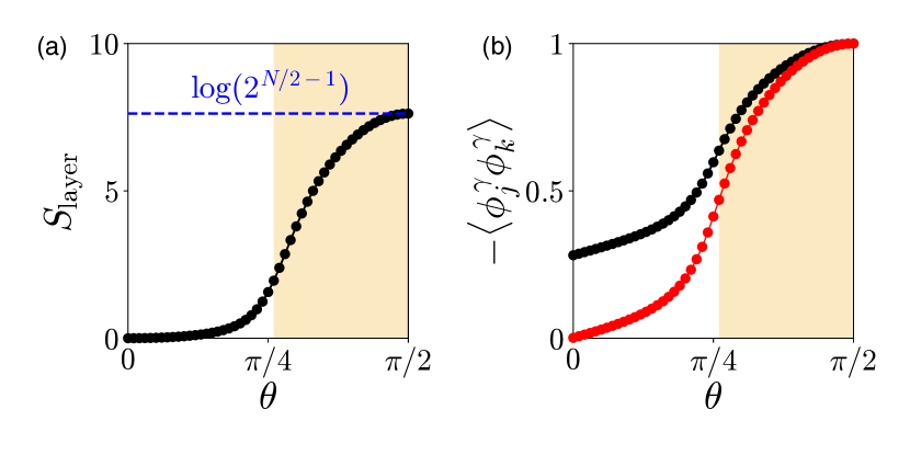
Figure 3: Results of the ED calculations. (a) The entanglement entropy $S_{\rm layer}$. The dashed line marks the value of $\log(2^{N/2-1})$, where $N=24$. (b) The spin-spin correlators for the hardcore dimer constraint. Black: $-\langle\phi_{j}^{\gamma}\phi_{k}^{\gamma}\rangle$. Red: $-\langle\phi_{j}^{\gamma}\phi_{k}^{\gamma}\rangle+\langle\sigma_{j}^{\gamma}\sigma_{k}^{\gamma}\rangle\langle\tau_{j}^{\gamma}\tau_{k}^{\gamma}\rangle$.

Exact diagonalization. The phase diagram of $H$ is studied via exact diagonalization (ED) on the (24+24)-site bilayer cluster in Fig. 1(a). We impose a periodic boundary condition and utilize the flux quantum numbers, $W_{p}=\pm 1$ & $Z_{p}=\pm 1$, to reduce the size of the Hilbert space in our ED calculations.

Figure 1(c) displays the resulting phase diagram. The KSL$\times$KSL and RVB states extend over large regions separated by a second order continuous transition at $\theta_{c}\simeq 0.26\pi$ (a small peak in the derivative of the ground state energy, $-\partial^{2}E_{\rm gs}/\partial\theta^{2}$). We check that both of the KSL$\times$KSL and RVB states appear in the uniform zero-flux sector ($W_{p}=Z_{p}=+1$). The two states are compared in terms of entanglement entropy, hardcore dimer constraint, and topological degeneracy below.

Quantum entanglement between the two layers is investigated by the entanglement entropy,

$$S_{\rm layer}=-\log({\rm Tr}_{\{\sigma\}}\rho_{\rm layer}^{2}),$$ (14)

where $\rho_{\rm layer}={\rm Tr}_{\{\tau\}}|\psi_{\rm gs}\rangle\langle\psi_{\rm gs}|$ is the reduced density matrix obtained by tracing out the $\tau$-spins in the ground state wave function $|\psi_{\rm gs}\rangle$. We find that $S_{\rm layer}\approx 0$ in the KSL$\times$KSL state, confirming that the state is simply a product state of two layers of KSL. By contrast, it approaches $S_{\rm layer}={\rm log}(2^{N/2-1})$ in the RVB state [Fig. 3(a)].

The hardcore dimer constraint in Eq. (9) is another good measure to distinguish between the KSL$\times$KSL and RVB states. Note that the two states show distinct behaviors: $\langle\phi_{j}^{\gamma}\phi_{k}^{\gamma}\rangle\approx\langle\sigma_{j}^{\gamma}\sigma_{k}^{\gamma}\rangle\langle\tau_{j}^{\gamma}\tau_{k}^{\gamma}\rangle$ in the KSL$\times$KSL state near $\theta=0$ and $\langle\phi_{j}^{\gamma}\phi_{k}^{\gamma}\rangle\approx-1$ in the RVB state around $\theta=\pi/2$. We measure the hardcore dimer constraint by evaluating the quantity,

$$-\langle\phi_{j}^{\gamma}\phi_{k}^{\gamma}\rangle+\langle\sigma_{j}^{\gamma}\sigma_{k}^{\gamma}\rangle\langle\tau_{j}^{\gamma}\tau_{k}^{\gamma}\rangle\approx\left\{\begin{array}[]{cc}0&({\rm KSL\times KSL})\\ 1&({\rm RVB})\end{array}\right..$$ (15)

We confirm this behavior in our ED calculations [see Fig. 3(b)].

Topological degeneracy is the ground state degeneracy on a torus geometry, which tells about the number of anyon types existing in each spin liquid phase Wen (1990); Wen and Niu (1990). We identify “ninefold” degeneracy in the KSL$\times$KSL phase and “fourfold” degeneracy in the RVB phase (Supplemental Material SM ).

Topological transition by anyon condensation. The degeneracy provides a supporting evidence for the underlying topological order of each phase. The ninefold degeneracy in the KSL$\times$KSL phase is consistent with the ${\rm Ising}\times\overline{\rm Ising}$ topological order with the nine different anyon-pairs, $\{1_{1},\sigma_{1},\psi_{1}\}\boxtimes\{1_{2},\sigma_{2},\psi_{2}\}$ Kitaev (2006); Burnell (2018). Here the subscript means the layer index (1: upper layer, 2: lower layer), and each layer has the three anyon sectors: trivial ($1$), vortex ($\sigma$), and fermion ($\psi$). On the other hand, the fourfold degeneracy in the RVB state implies the toric code $\mathbb{Z}_{2}$ topological order with the four different anyons, $\{1,e,m,\epsilon\}$; the $e$- and $m$-particles are bosons with mutual statistics, and the $\epsilon$-particle is a fermion composed of the $e$- and $m$-particles Kitaev (2003, 2006).

The transition between the ${\rm Ising}\times\overline{\rm Ising}$ and $\mathbb{Z}_{2}$ topological orders has been conceptually understood by anyon condensation Bais and Slingerland (2009); Burnell et al. (2011, 2012); Burnell (2018). Suppose we condense the fermion-pair $\psi_{1}\boxtimes\psi_{2}$. Then, $\psi_{1}\boxtimes 1_{2}$ and $1_{1}\boxtimes\psi_{2}$ become indistinguishable and identified as a same type of anyons in the condensed phase. Moreover, anyons having nontrivial braiding with the fermions are confined, and only $\psi_{1}\boxtimes 1_{2}$, $1_{1}\boxtimes\psi_{2}$, and $\sigma_{1}\boxtimes\sigma_{2}$ remain deconfined. We note that

$$(\sigma_{1}\boxtimes\sigma_{2})\times(\sigma_{1}\boxtimes\sigma_{2})$$ (16)

$$= (1_{1}\boxtimes 1_{2})+(\psi_{1}\boxtimes 1_{2})+(1_{1}\boxtimes\psi_{2})+(\psi_{1}\boxtimes\psi_{2}),~{}~{}~{}~{}~{}~{}~{}$$

where we have two trivial anyons ($1_{1}\boxtimes 1_{2}$,$\psi_{1}\boxtimes\psi_{2}$) and two fermions ($\psi_{1}\boxtimes 1_{2}$,$1_{1}\boxtimes\psi_{2}$). Therefore, $\sigma_{1}\boxtimes\sigma_{2}$ must be split into two anyons in the condensed phase. We assume that

$$\sigma_{1}\boxtimes\sigma_{2}\equiv e+m,~{}~{}\psi_{1}\boxtimes 1_{2}\equiv 1_{1}\boxtimes\psi_{2}\equiv\epsilon,~{}~{}1_{1}\boxtimes 1_{2}\equiv 1.$$ (17)

Then, Eq. (16) leads to the toric code’s fusion rules: $e\times e=1$, $m\times m=1$, $e\times m=m\times e=\epsilon$ Burnell (2018).

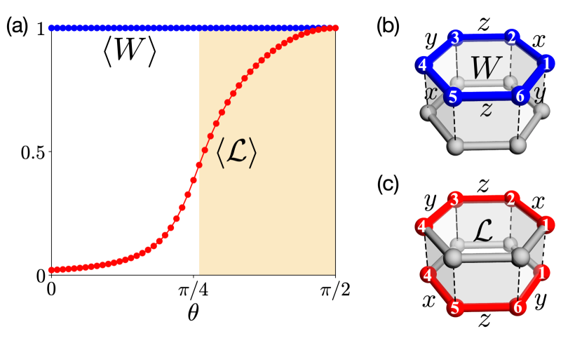
Figure 4: Anyon condensation. (a) The expectation values of the loop operators, $\langle W\rangle$ and $\langle\mathcal{L}\rangle$. (b),(c) Visualizations of the $W$ and $\mathcal{L}$ operators.

The mechanism of the anyon condensate induced transition is tested by our microscopic model calculations. We consider two different loop operators. The first one is the usual hexagon plaquette operator,

$$W=(\sigma_{1}^{y}\sigma_{6}^{y})(\sigma_{6}^{z}\sigma_{5}^{z})(\sigma_{5}^{x}\sigma_{4}^{x})(\sigma_{4}^{y}\sigma_{3}^{y})(\sigma_{3}^{z}\sigma_{2}^{z})(\sigma_{2}^{x}\sigma_{1}^{x}),$$ (18)

which is defined within a single layer [Fig. 4(b)]. If we apply the Majorana representation, $\sigma_{j}^{\gamma}\sigma_{k}^{\gamma}=-u_{jk}(ic_{j}c_{k})$ where $u_{jk}=ib_{j}^{\gamma}b_{k}^{\gamma}$, the action of $W$ is to create a pair of $c$-fermions, move one of the fermions along the hexagon, and finally annihilate the fermion-pair Kitaev (2006). Notice that the $c$-fermions correspond to $\psi_{1}$ fermions. The second one is defined over the two layers:

$$\mathcal{L}=-(\tau_{1}^{y}\tau_{6}^{y})(\tau_{6}^{z}\tau_{5}^{z})(\tau_{5}^{x}\tau_{4}^{x})(\sigma_{4}^{y}\sigma_{3}^{y})(\sigma_{3}^{z}\sigma_{2}^{z})(\sigma_{2}^{x}\sigma_{1}^{x}).$$ (19)

This operator moves a fermion ($\psi_{1}$) around an upper “half” hexagon, and moves another fermion ($\psi_{2}$) around a lower “half” hexagon [Fig. 4(c)]. This type of loop operator has been considered in Ref. Wang et al. (2021).

Figure 4(a) shows the expectation value $\langle\mathcal{L}\rangle$. We find that $\langle\mathcal{L}\rangle$ stays small in the KSL$\times$KSL phase (close to zero near $\theta=0$), meaning that $\psi_{1}$ and $\psi_{2}$ cannot move across the two layers because they are distinct anyons supported on different layers.

By contrast, we see substantially large $\langle\mathcal{L}\rangle$ in the RVB phase (reaching one at $\theta=\pi/2$). This implies that $\psi_{1}$ and $\psi_{2}$ become indistinguishable, thus the fermions ($\psi_{1}\equiv\psi_{2}$) can complete the hexagon loop motion. This is only possible when we have the condensation of $\psi_{1}\boxtimes\psi_{2}$. Therefore, $\langle\mathcal{L}\rangle$ plays a role of an order parameter for the anyon condensation.

Discussions. The anyon condensation transition between the ${\rm Ising}\times\overline{\rm Ising}$ and $\mathbb{Z}_{2}$ topological orders was measured in our ED calculations via the loop operator $\mathcal{L}$. Interestingly, there is an intimate relationship between the anyon condensation and the hardcore dimer constraint [Eq. (9)]. To see this, we consider the constraint in a slightly different fashion: $\sigma_{j}^{\gamma}\sigma_{k}^{\gamma}=-\tau_{j}^{\gamma}\tau_{k}^{\gamma}$. This tells us that moving the fermions, $\psi_{1}$ & $\psi_{2}$, have a same effect, meaning that the RVB state does not distinguish between $\psi_{1}$ and $\psi_{2}$; they are essentially same particles. To be more precise, if we apply the hardcore dimer constraint to Eq. (19), we obtain the relationship $\mathcal{L}=W=Z$. Therefore, the hardcore dimer constraint itself means the $\psi_{1}\boxtimes\psi_{2}$ anyon condensation.

Low energy field theory for the transition is an interesting problem lying beyond the Landau-Ginzburg-Wilson paradigm. To our best knowledge, a general framework for such transitions is currently unknown Burnell (2018). Nonetheless, the (2+1)D transverse field Ising universality has been proposed for the $\psi_{1}\boxtimes\psi_{2}$ condensate induced transition between the ${\rm Ising}\times\overline{\rm Ising}$ and $\mathbb{Z}_{2}$ topological orders by Burnell, Simon, and Slingerland Burnell et al. (2012, 2011). Our system is expected to be in the same 3D Ising universality class, which is supported by our estimation of the critical exponent $\beta\approx 0.3$ SM .

Our bilayer spin model is compared with the recent spin-$3/2$ transverse field Ising model by Verresen and Vishwanath Verresen and Vishwanath (2022). Both cases lead to emergent quantum dimer models with similar structures. The hardcore dimer constraint for the Hilbert space is energetically implemented, and the dimer resonance is induced by anyon fluctuations—by the Kitaev interactions in our case, and by the transverse field in their case. Despite the similarities, the two works have different interests. Ref. Verresen and Vishwanath (2022) focuses on the possible quantum liquids induced by different types of anyon fluctuations. In our study, we are mainly interested in anyon condensation transition and its identification.

Our model can be generalized to any tri-coordinated lattices beyond the honeycomb lattice like the Kitaev model Yang et al. (2007). The star lattice would be an interesting case where the Kitaev model allows a chiral spin liquid Yao and Kivelson (2007). Such spontaneous time reversal breaking may also impact on the RVB side and the allowed anyon types. It would be a promising direction to extend this study to other lattice geometries.

I am grateful to Eun-Gook Moon for invaluable discussions. I thank Onur Erten for introducing a related work about Kitaev spin-orbital bilayer models Nica et al. (2023). Computations were performed on clusters at the Center for Advanced Computation (CAC) of Korea Institute for Advanced Study (KIAS). This work was supported by KIAS Individual Grants (No. PG071402 & PG071403).

Supplemental Material on “Topological Quantum Dimers Emerging from Kitaev Spin Liquid Bilayer: Anyon Condensation Transition”

I Perturbation theory for the strong coupling limit

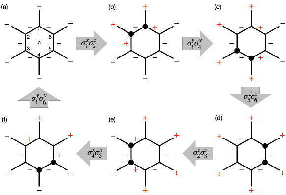
Figure S1: A sixth order perturbation. The signs indicate the value of $\phi_{j}^{\gamma}\phi_{k}^{\gamma}(=\pm 1)$ at each bond. (a) An initial ground state $|\Phi^{\prime}\rangle$. (b) The intermediate state $|\nu\rangle=(K_{\sigma}\sigma_{1}^{x}\sigma_{2}^{x}+K_{\tau}\tau_{1}^{x}\tau_{2}^{x})|\Phi^{\prime}\rangle=2K_{\sigma}\sigma_{1}^{x}\sigma_{2}^{x}|\Phi^{\prime}\rangle$. (c) The next intermediate state $|\mu\rangle=(K_{\sigma}\sigma_{3}^{y}\sigma_{4}^{y}+K_{\tau}\tau_{3}^{y}\tau_{4}^{y})|\nu\rangle=2K_{\sigma}\sigma_{3}^{y}\sigma_{4}^{y}|\nu\rangle$. Similarly for other intermediate states $|\rho\rangle,|\beta\rangle,|\alpha\rangle$ in (d),(e),(f). After all the Kitaev interactions around the plaquette $p$, the state comes back to some other ground state $|\Phi\rangle$.

To investigate the strong coupling limit, we separate the Hamiltonian into the two parts, $H=H_{0}+H^{\prime}$, where $H_{0}=\sum_{\langle jk\rangle_{\gamma}}G\phi_{j}^{\gamma}\phi_{k}^{\gamma}$, and $H^{\prime}=\sum_{\langle jk\rangle_{\gamma}}K_{\sigma}\sigma_{j}^{\gamma}\sigma_{k}^{\gamma}+K_{\tau}\tau_{j}^{\gamma}\tau_{k}^{\gamma}$. Remember that we focus on the parameter region of $G>0~{}\&~{}K_{\tau}=-K_{\sigma}$. The ground state manifold of $H_{0}$ is extensively degenerate and characterized by the constraint, $\phi_{j}^{\gamma}\phi_{k}^{\gamma}=-1$, at each bond. Note that the eigenstates of the composite spin operators $\{\phi_{j}^{\gamma}\}$ are automatically the energy eigenstates of $H_{0}$. In this basis, we find that the action of each Kitaev term of $H^{\prime}$ is determined by the value of $\phi_{j}^{\gamma}\phi_{k}^{\gamma}$:

$$(K_{\sigma}\sigma_{j}^{\gamma}\sigma_{k}^{\gamma}+K_{\tau}\tau_{j}^{\gamma}\tau_{k}^{\gamma})|\Phi\rangle=\left\{\begin{array}[]{cc}2K_{\sigma}\sigma_{j}^{\gamma}\sigma_{k}^{\gamma}|\Phi\rangle&({\rm when}~{}~{}\phi_{j}^{\gamma}\phi_{k}^{\gamma}=-1)\\ 0&({\rm when}~{}~{}\phi_{j}^{\gamma}\phi_{k}^{\gamma}=+1)\end{array}\right\},$$ (S1)

where $|\Phi\rangle$ is an arbitrary state of $\{\phi_{j}^{\gamma}\}$.

The effective Hamiltonian $\mathcal{H}_{\rm eff}$ for the ground state manifold is constructed by a degenerate perturbation theory Winkler (2003). Nontrivial interaction terms (other than constant energy shifts) arise at the sixth order perturbations:

$$\langle\Phi|\mathcal{H}_{\rm eff}|\Phi^{\prime}\rangle = \frac{1}{2}\sum_{\alpha,\beta,\rho,\mu,\nu}\frac{\langle\Phi|H^{\prime}|\alpha\rangle\langle\alpha|H^{\prime}|\beta\rangle\langle\beta|H^{\prime}|\rho\rangle\langle\rho|H^{\prime}|\mu\rangle\langle\mu|H^{\prime}|\nu\rangle\langle\nu|H^{\prime}|\Phi^{\prime}\rangle}{(E_{\Phi}^{(0)}-E_{\alpha}^{(0)})(E_{\Phi}^{(0)}-E_{\beta}^{(0)})(E_{\Phi}^{(0)}-E_{\rho}^{(0)})(E_{\Phi}^{(0)}-E_{\mu}^{(0)})(E_{\Phi}^{(0)}-E_{\nu}^{(0)})}$$ (S2)

$$+ \frac{1}{2}\sum_{\alpha,\beta,\rho,\mu,\nu}\frac{\langle\Phi|H^{\prime}|\alpha\rangle\langle\alpha|H^{\prime}|\beta\rangle\langle\beta|H^{\prime}|\rho\rangle\langle\rho|H^{\prime}|\mu\rangle\langle\mu|H^{\prime}|\nu\rangle\langle\nu|H^{\prime}|\Phi^{\prime}\rangle}{(E_{\Phi^{\prime}}^{(0)}-E_{\alpha}^{(0)})(E_{\Phi^{\prime}}^{(0)}-E_{\beta}^{(0)})(E_{\Phi^{\prime}}^{(0)}-E_{\rho}^{(0)})(E_{\Phi^{\prime}}^{(0)}-E_{\mu}^{(0)})(E_{\Phi^{\prime}}^{(0)}-E_{\nu}^{(0)}),}$$

where $|\Phi\rangle$ and $|\Phi^{\prime}\rangle$ are states in the ground state manifold, $H_{0}|\Phi\rangle=E_{\Phi}^{(0)}|\Phi\rangle$, $H_{0}|\Phi^{\prime}\rangle=E_{\Phi^{\prime}}^{(0)}|\Phi^{\prime}\rangle$, and similarly for the intermediate states, $|\alpha\rangle$, $|\beta\rangle$, $|\rho\rangle$, $|\mu\rangle$, $|\nu\rangle$. Figure S1 illustrates one example (among various possible sixth order processes): we act the Kitaev terms, $K_{\sigma}\sigma_{j}^{\gamma}\sigma_{k}^{\gamma}+K_{\tau}\tau_{j}^{\gamma}\tau_{k}^{\gamma}$, along a plaquette $p$ using Eq. (S1). Its contribution to $\mathcal{H}_{\rm eff}$ is given by the expression,

$$\frac{(2K_{\sigma})^{6}\langle\Phi|\sigma_{1}^{y}\sigma_{6}^{y}|\alpha\rangle\langle\alpha|\sigma_{4}^{x}\sigma_{5}^{x}|\beta\rangle\langle\beta|\sigma_{2}^{z}\sigma_{3}^{z}|\rho\rangle\langle\rho|\sigma_{5}^{z}\sigma_{6}^{z}|\mu\rangle\langle\mu|\sigma_{3}^{y}\sigma_{4}^{y}|\nu\rangle\langle\nu|\sigma_{1}^{x}\sigma_{2}^{x}|\Phi^{\prime}\rangle}{(-4G)(-6G)(-6G)(-6G)(-4G)}=-\frac{1}{54}\frac{K_{\sigma}^{6}}{G^{5}}\langle\Phi|\hat{W}_{p}|\Phi^{\prime}\rangle.$$ (S3)

Collecting all the sixth order contributions, we obtain the effective Hamiltonian,

$$\mathcal{H}_{\rm eff}=-\lambda\sum_{p}\hat{W}_{p},$$ (S4)

where $\lambda\propto K_{\sigma}^{6}/G^{5}$.

II Quantum dimer model

Dimer motion graph	$f(\mathpzc{D})$
	1
	-1

Table SI: Dimer motion graphs of $\hat{W}_{p}$ and the sign factor $f(\mathpzc{D})$. Each graph depicts a dimer configuration (red) and the closed path (light blue) of the dimer motions by $\hat{W}_{p}$. Other cases related by symmetry are dropped for simplicity.

In the dimer representation, the effective Hamiltonian $\mathcal{H}_{\rm eff}$ has the interpretation of dimer resonance motions. The dimer Hilbert space is provided by the ground states of $H_{0}$ respecting the hardcore dimer constraint. Acting on the hardcore dimer states, a plaquette operator $\hat{W}_{p}$ generates dimer motions along closed paths around the plaquette $p$. For example, pinwheel dimers are moved along the path of 12-site David star:

$$= |t_{x}\rangle_{1}\otimes|t_{z}\rangle_{2}\otimes|t_{y}\rangle_{3}\otimes|t_{x}\rangle_{4}\otimes|t_{z}\rangle_{5}\otimes|t_{y}\rangle_{6}$$ (S5)

$$\xrightarrow{\hat{W}_{p}} \sigma_{1}^{z}|t_{x}\rangle_{1}\otimes\sigma_{2}^{y}|t_{z}\rangle_{2}\otimes\sigma_{3}^{x}|t_{y}\rangle_{3}\otimes\sigma_{4}^{z}|t_{x}\rangle_{4}\otimes\sigma_{5}^{y}|t_{z}\rangle_{5}\otimes\sigma_{6}^{x}|t_{y}\rangle_{6}$$

$$= i|t_{y}\rangle_{1}\otimes i|t_{x}\rangle_{2}\otimes i|t_{z}\rangle_{3}\otimes i|t_{y}\rangle_{4}\otimes i|t_{x}\rangle_{5}\otimes i|t_{z}\rangle_{6}=(-1)\parbox{36.98866pt}{\includegraphics[width=433.62pt]{./pinwheel2.pdf}}.$$

Notice that the resulting dimer state is accompanied with an extra minus sign. On the other hand, hexagon dimers are shifted along the path of 6-site hexagon:

$$= |t_{z}\rangle_{1}\otimes|s\rangle_{2}\otimes|t_{x}\rangle_{3}\otimes|s\rangle_{4}\otimes|t_{y}\rangle_{5}\otimes|s\rangle_{6}$$ (S6)

$$\xrightarrow{\hat{W}_{p}} \sigma_{1}^{z}|t_{z}\rangle_{1}\otimes\sigma_{2}^{y}|s\rangle_{2}\otimes\sigma_{3}^{x}|t_{x}\rangle_{3}\otimes\sigma_{4}^{z}|s\rangle_{4}\otimes\sigma_{5}^{y}|t_{y}\rangle_{5}\otimes\sigma_{6}^{x}|s\rangle_{6}$$

$$= |s\rangle_{1}\otimes|t_{y}\rangle_{2}\otimes|s\rangle_{3}\otimes|t_{z}\rangle_{4}\otimes|s\rangle_{5}\otimes|t_{x}\rangle_{6}=\parbox{36.98866pt}{\includegraphics[width=433.62pt]{./hexagon2.pdf}}.$$

In this case, there is no sign change. Repeating the same calculations for other dimer configurations, we obtain the dimer model,

$$\hat{W}_{p}=\sum_{\mathpzc{D}}f(\mathpzc{D})|\mathpzc{D}\rangle\langle\bar{\mathpzc{D}}|+{\rm H.c.},$$ (S7)

where $\mathpzc{D}$ runs over 32 distinct dimer configurations around the local plaquette $p$, and $|\bar{\mathpzc{D}}\rangle$ means the conjugate dimer configuration of $|\mathpzc{D}\rangle$ connected by $\hat{W}_{p}$. The full list of the dimer motions and the associated sign factor $f(\mathpzc{D})$ are described in Table SI.

III General cases beyond Eq. (3)

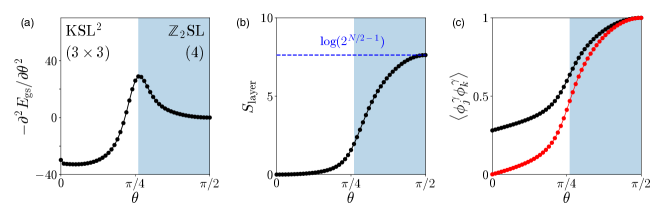
Figure S2: ED results for the case #5 and #6. (a) Phase diagram of the model. The KSL$\times$KSL and $\mathbb{Z}_{2}{\rm SL}$ states are connected by a second order continuous transition at $\theta_{c}\simeq 0.26\pi$ as indicated by a small peak in the derivative of the ground state energy, $-{\partial^{2}E_{\rm gs}}/{\partial\theta^{2}}$. The numbers in the parentheses indicate topological degeneracy. (b) The entanglement entropy $S_{\rm layer}$. The dashed line marks the value of $\log(2^{N/2-1})$, where $N=24$. (c) The spin-spin correlators, $\langle\phi_{j}^{\gamma}\phi_{k}^{\gamma}\rangle$ (black) and $\langle\phi_{j}^{\gamma}\phi_{k}^{\gamma}\rangle-\langle\sigma_{j}^{\gamma}\sigma_{k}^{\gamma}\rangle\langle\tau_{j}^{\gamma}\tau_{k}^{\gamma}\rangle$ (red). Exactly same results of $E_{\rm gs}$, $S_{\rm layer}$, $\langle\phi_{j}^{\gamma}\phi_{k}^{\gamma}\rangle$, $\langle\phi_{j}^{\gamma}\phi_{k}^{\gamma}\rangle-\langle\sigma_{j}^{\gamma}\sigma_{k}^{\gamma}\rangle\langle\tau_{j}^{\gamma}\tau_{k}^{\gamma}\rangle$ are obtained for both cases (#5,6).

In the bilayer model [Eq. (1)], the emergence of a RVB-type $\mathbb{Z}_{2}$ spin liquid is determined by the signs of all the couplings $\{G,K_{\sigma},K_{\tau}\}$. Table SII summarizes six possible cases for the sign structure of $\{G,K_{\sigma},K_{\tau}\}$. We find that three cases (#1,5,6) stabilize a $\mathbb{Z}_{2}$ spin liquid ($\mathbb{Z}_{2}$SL) whereas the other three cases do not. The case #1 corresponds to the parameter choice in Eq. (3).

Case	$G$	$K_{\sigma}$	$K_{\tau}$	$\mathbb{Z}_{2}$ spin liquid
#1	$+$	$+$	$-$	✓
#2	$+$	$+$	$+$
#3	$+$	$-$	$-$
#4	$-$	$+$	$-$
#5	$-$	$+$	$+$	✓
#6	$-$	$-$	$-$	✓

Table SII: Possible sign structures of the coupling constants $\{G,K_{\sigma},K_{\tau}\}$ and the emergence of a RVB-type $\mathbb{Z}_{2}$ spin liquid state.

Here we discuss the case #5 and #6 ($G<0,~{}K_{\sigma}=K_{\tau}$). Figure S2 shows the ED results for the two cases with the parametrization,

$$G=-\sin\theta~{}~{}~{}\&~{}~{}~{}K_{\sigma}=K_{\tau}=\left\{\begin{array}[]{cc}+\cos\theta&({\rm Case~{}\#5})\\ -\cos\theta&({\rm Case~{}\#6})\end{array}\right\}.$$ (S8)

The results are almost same as in the case #1 in terms of the ground state energy $E_{\rm gs}$, the topological degeneracy, the entanglement entropy $S_{\rm layer}$, and the spin-spin correlator $\langle\phi_{j}^{\gamma}\phi_{k}^{\gamma}\rangle$. Yet, there is a difference between #5,6 and #1 in the sign of $\langle\phi_{j}^{\gamma}\phi_{k}^{\gamma}\rangle$, which is positive in the former cases but negative in the latter case. In the strong coupling limit ($|G|\gg|K_{\sigma,\tau}|$), we see distinct behaviors in the associated $\mathbb{Z}_{2}$ spin liquids:

$$\langle\phi_{j}^{\gamma}\phi_{k}^{\gamma}\rangle\rightarrow\left\{\begin{array}[]{cc}+1&({\rm Case~{}\#5,6})\\ -1&({\rm Case~{}\#1})\end{array}\right\}.$$ (S9)

The property $\phi_{j}^{\gamma}\phi_{k}^{\gamma}=-1$ of #1 corresponds to the hardcore dimer constraint in the dimer picture. However, the property $\phi_{j}^{\gamma}\phi_{k}^{\gamma}=+1$ of #5,6 leads to states violating the hardcore dimer constraint. Because of the property of #5,6, a $\mathbb{Z}_{2}$ gauge theory description is naturally constructed rather than the dimer model description Nica et al. (2023).

In the other cases (#2,3,4), the effects of the $K_{\sigma,\tau}$ terms completely cancel each other, failing to create any $\mathbb{Z}_{2}$ spin liquid state in the strong coupling limit. For instance, in the case #2 and #3 ($G>0$ and $K_{\sigma}=K_{\tau}$), we can easily see the cancellation from the relationship,

$$\sigma_{j}^{\gamma}\sigma_{k}^{\gamma}|\Phi\rangle=-\tau_{j}^{\gamma}\tau_{k}^{\gamma}|\Phi\rangle,$$ (S10)

where $|\Phi\rangle$ is an arbitrary dimer state satisfying the hardcore dimer constraint, $\phi_{j}^{\gamma}\phi_{k}^{\gamma}=-1$ (required by the interlayer coupling). If the $K_{\sigma,\tau}$ terms are applied to the dimer state, one can find that

$$(K_{\sigma}\sigma_{j}^{\gamma}\sigma_{k}^{\gamma}+K_{\tau}\tau_{j}^{\gamma}\tau_{k}^{\gamma})|\Phi\rangle=(K_{\sigma}-K_{\tau})\sigma_{j}^{\gamma}\sigma_{k}^{\gamma}|\Phi\rangle=0.$$ (S11)

Due to this cancellation, the Kitaev interactions do not create any effect on the dimer Hilbert space and any $\mathbb{Z}_{2}$ spin liquid.

IV Majorana mean-field theory for the weak coupling limit

To construct an effective theory for the weak coupling limit ($|G|\ll|K_{\sigma,\tau}|$), we arrange the Hamiltonian into the form $H=H_{0}+H_{1}$ (where $H_{0}=\sum_{\langle jk\rangle_{\gamma}}K_{\sigma}\sigma_{j}^{\gamma}\sigma_{k}^{\gamma}+K_{\tau}\tau_{j}^{\gamma}\tau_{k}^{\gamma}$ and $H_{1}=G\sum_{\langle jk\rangle_{\gamma}}\sigma_{j}^{\gamma}\sigma_{k}^{\gamma}\tau_{j}^{\gamma}\tau_{k}^{\gamma}$), and perform a second order perturbation theory. The resulting effective Hamiltonian is given by

$$\mathcal{H}_{\rm eff}(G\ll K)=H_{0}+H_{1}-\frac{1}{\Delta E}H_{1}H_{1},$$ (S12)

where $\Delta E(\propto|K_{\sigma}|)$ means the energy difference between the ground state and an intermediate excited state of $H_{0}$. Nontrivial effects are generated by the second order term,

$$-\frac{1}{\Delta E}H_{1}H_{1}\propto-\frac{G^{2}}{|K_{\sigma}|}\sum_{\langle ij\rangle_{\alpha}}\sigma_{i}^{\alpha}\sigma_{j}^{\alpha}\tau_{i}^{\alpha}\tau_{j}^{\alpha}\sum_{\langle kl\rangle_{\gamma}}\sigma_{k}^{\gamma}\sigma_{l}^{\gamma}\tau_{k}^{\gamma}\tau_{l}^{\gamma}.$$ (S13)

Among the various combinations of spin operators, we are particularly interested in the combinations that are defined on connected two bonds. For instance, $(\sigma_{1}^{x}\sigma_{2}^{x}\tau_{1}^{x}\tau_{2}^{x})(\sigma_{2}^{y}\sigma_{3}^{y}\tau_{2}^{y}\tau_{3}^{y})$ on adjacent two bonds, $\langle 12\rangle_{x}$ and $\langle 23\rangle_{y}$. This eight-spin operator can be simplified to a six-spin operator:

$$(\sigma_{1}^{x}\sigma_{2}^{x}\tau_{1}^{x}\tau_{2}^{x})(\sigma_{2}^{y}\sigma_{3}^{y}\tau_{2}^{y}\tau_{3}^{y})=(\sigma_{1}^{x}\underbrace{\sigma_{2}^{x}\sigma_{2}^{y}}_{i\sigma_{2}^{z}}\sigma_{3}^{y})(\tau_{1}^{x}\underbrace{\tau_{2}^{x}\tau_{2}^{y}}_{i\tau_{2}^{z}}\tau_{3}^{y})=-(\sigma_{1}^{x}\sigma_{2}^{z}\sigma_{3}^{y})(\tau_{1}^{x}\tau_{2}^{z}\tau_{3}^{y}).$$ (S14)

By collecting this kind of terms, we arrange the effective Hamiltonian in the following form.

$$\mathcal{H}_{\rm eff}(G\ll K)=H_{0}+\eta\sum_{\langle ij\rangle_{\alpha}\langle jk\rangle_{\gamma}}\sigma_{i}^{\alpha}\sigma_{j}^{\beta}\sigma_{k}^{\gamma}\tau_{i}^{\alpha}\tau_{j}^{\beta}\tau_{k}^{\gamma}+\cdots,$$ (S15)

where $\eta(\propto G^{2}/|K_{\sigma}|)$ is a positive constant, and the summation is for all possible combinations of connected two bonds, $\langle ij\rangle_{\alpha}\langle jk\rangle_{\gamma}$.

The effective Hamiltonian is solved by a mean-field theory. To the six-spin operators, we apply the mean-field decoupling,

$$\sigma_{i}^{\alpha}\sigma_{j}^{\beta}\sigma_{k}^{\gamma}\tau_{i}^{\alpha}\tau_{j}^{\beta}\tau_{k}^{\gamma}\rightarrow\sigma_{i}^{\alpha}\sigma_{j}^{\beta}\sigma_{k}^{\gamma}\langle\tau_{i}^{\alpha}\tau_{j}^{\beta}\tau_{k}^{\gamma}\rangle+\langle\sigma_{i}^{\alpha}\sigma_{j}^{\beta}\sigma_{k}^{\gamma}\rangle\tau_{i}^{\alpha}\tau_{j}^{\beta}\tau_{k}^{\gamma}-\langle\sigma_{i}^{\alpha}\sigma_{j}^{\beta}\sigma_{k}^{\gamma}\rangle\langle\tau_{i}^{\alpha}\tau_{j}^{\beta}\tau_{k}^{\gamma}\rangle.$$ (S16)

Similar mean-field decoupling schemes may be applied to the other terms that are not explicitly shown in Eq. (S15). Yet, those terms merely renormalize the Kitaev term $H_{0}$. Hence, we ignore those terms and just focus on the mean-field Hamiltonian

$$\mathcal{H}_{\rm MF}=H_{0}+\eta\sum_{\langle ij\rangle_{\alpha}\langle jk\rangle_{\gamma}}\left[\sigma_{i}^{\alpha}\sigma_{j}^{\beta}\sigma_{k}^{\gamma}\langle\tau_{i}^{\alpha}\tau_{j}^{\beta}\tau_{k}^{\gamma}\rangle+\langle\sigma_{i}^{\alpha}\sigma_{j}^{\beta}\sigma_{k}^{\gamma}\rangle\tau_{i}^{\alpha}\tau_{j}^{\beta}\tau_{k}^{\gamma}-\langle\sigma_{i}^{\alpha}\sigma_{j}^{\beta}\sigma_{k}^{\gamma}\rangle\langle\tau_{i}^{\alpha}\tau_{j}^{\beta}\tau_{k}^{\gamma}\rangle\right].$$ (S17)

The three-spin terms, $\sigma_{i}^{\alpha}\sigma_{j}^{\beta}\sigma_{k}^{\gamma}$ & $\tau_{i}^{\alpha}\tau_{j}^{\beta}\tau_{k}^{\gamma}$, break time reversal and create a finite energy gap in the fermion excitations of the Kitaev spin liquid state Kitaev (2006).

We now employ the Kitaev’s Majorana representation for spin-1/2 operator Kitaev (2006),

$$\sigma_{i}^{\alpha}=ib_{1,i}^{\alpha}c_{1,i}~{}~{}~{}\&~{}~{}~{}\tau_{i}^{\alpha}=ib_{2,i}^{\alpha}c_{2,i},$$ (S18)

where the subscript (1,2) means the upper/lower layer. This representation leads to the Majorana mean-field Hamiltonian,

$$\mathcal{H}_{\rm MF}=\sum_{\langle ij\rangle}\left[(-K_{\sigma})ic_{1,i}c_{1,j}+(-K_{\tau})ic_{2,i}c_{2,j}\right]+\sum_{\langle\langle ik\rangle\rangle}\left[(\eta M_{2})ic_{1,i}c_{1,k}+(\eta M_{1})ic_{2,i}c_{2,k}-\eta M_{1}M_{2}\right],$$ (S19)

where we have chosen the simplest gauge for the uniform zero-flux ($u_{1,ij}=ib_{1,i}^{\alpha}b_{1,j}^{\alpha}=+1$ and $u_{2,ij}=ib_{2,i}^{\alpha}b_{2,j}^{\alpha}=+1$ with site $i$ in A sublattice and $j$ in B sublattice), and introduced the mean-field parameters,

$$M_{1}=\langle ic_{1,i}c_{1,k}\rangle~{}~{}~{}\&~{}~{}~{}M_{2}=\langle ic_{2,i}c_{2,k}\rangle.$$ (S20)

In this mean-field theory, the two layers are only coupled by the mean-field parameters, $M_{1}$ and $M_{2}$.

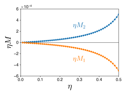
Figure S3: Result of the Majorana mean-field theory. The mean-field parameters ($M_{1,2}$) are obtained by solving Eq. (S20) self-consistently. The Kitaev term is fixed by $|K_{\sigma}|=|K_{\tau}|=1$. The result does not depend on the relative sign of the coupling constants.

Figure S3 shows the result of the self-consistent mean-field calculations. We find that the mean-field parameters have a same magnitude but the opposite signs ($M_{1}=-M_{2}$). This implies that the KSL state of each layer ($1,2$) has a finite energy gap $\Delta_{1,2}=6\sqrt{3}|\eta M_{2,1}|$ and the nonzero Chern number $\nu_{1,2}={\rm sgn}(\eta M_{2,1})=\pm 1$ Kitaev (2006). More importantly, the two layers have the opposite signs for the Chern number (e.g., $\nu_{1}=+1$ & $\nu_{2}=-1$). This mean-field theory shows that the KSL$\times$KSL state has the ${\rm Ising}\times\overline{\rm Ising}$ topological order Kitaev (2006); Burnell (2018).

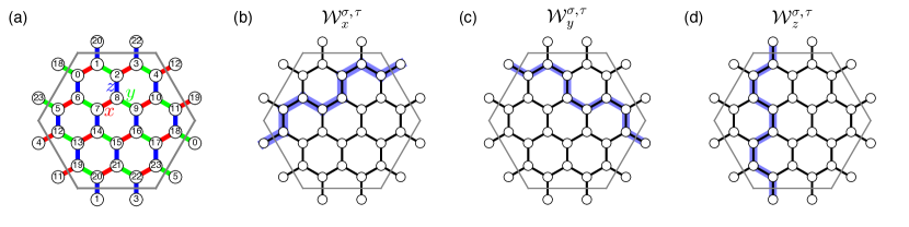
Figure S4: Wilson loop operators on the finite size cluster. (a) The 24-site cluster with four state per site and periodic boundary condition. (b),(c),(d) Visualizations of the Wilson loop operators, $\mathcal{W}_{x}^{\sigma,\tau}$, $\mathcal{W}_{y}^{\sigma,\tau}$, $\mathcal{W}_{z}^{\sigma,\tau}$.

V Topological degeneracy

To facilitate the analysis of topological degeneracy, we employ four Wilson loop operators, $\{\mathcal{W}_{x}^{\sigma},\mathcal{W}_{y}^{\sigma},\mathcal{W}_{x}^{\tau},\mathcal{W}_{y}^{\tau}\}$, commuting with $H$. The Hilbert space can then be partitioned into sixteen sectors distinguished by the eigenvalues of the Wilson loop operators ($\mathcal{W}_{x,y}^{\sigma,\tau}=\pm 1$).

The Wilson loop operators are defined by generalizing the hexagon plaquette operators ($\hat{W}_{p}$,$\hat{Z}_{p}$) to non-contractible loops of the system on a torus geometry. Figure S4(a) shows the cluster used in our exact diagonalization study. We impose a periodic boundary condition across the gray hexagon. Along the non-contractible loop in Fig. S4(b), we define the Wilson operator $\mathcal{W}_{x}^{\sigma}$ as follows.

$$\mathcal{W}_{x}^{\sigma} = (\sigma_{12}^{z}\sigma_{5}^{z})(\sigma_{5}^{x}\sigma_{6}^{x})(\sigma_{6}^{y}\sigma_{7}^{y})(\sigma_{7}^{x}\sigma_{8}^{x})(\sigma_{8}^{z}\sigma_{2}^{z})(\sigma_{2}^{x}\sigma_{3}^{x})(\sigma_{3}^{y}\sigma_{4}^{y})(\sigma_{4}^{x}\sigma_{12}^{x})$$ (S21)

$$= -\sigma_{12}^{y}\sigma_{5}^{y}\sigma_{6}^{z}\sigma_{7}^{z}\sigma_{8}^{y}\sigma_{2}^{y}\sigma_{3}^{z}\sigma_{4}^{z}.$$

This is nothing but the product of the Kitaev terms of $\sigma$-spins along the non-contractible loop. Repeating for other possible non-contractible loops [Fig. S4(c),(d)], we can define other Wilson loop operators:

$$\mathcal{W}_{y}^{\sigma}=-\sigma_{0}^{z}\sigma_{1}^{z}\sigma_{2}^{x}\sigma_{8}^{x}\sigma_{9}^{z}\sigma_{10}^{z}\sigma_{11}^{x}\sigma_{18}^{x},$$ (S22)

$$\mathcal{W}_{z}^{\sigma}=-\sigma_{1}^{y}\sigma_{0}^{y}\sigma_{6}^{x}\sigma_{7}^{x}\sigma_{14}^{y}\sigma_{13}^{y}\sigma_{19}^{x}\sigma_{20}^{x}.$$ (S23)

Note that the three operators satisfy the relationship, $\mathcal{W}_{x}^{\sigma}\mathcal{W}_{y}^{\sigma}\mathcal{W}_{z}^{\sigma}=+1$, in the ground state manifold because of the property of uniform zero-flux ($W_{p}=Z_{p}=+1$). Among the three operators, we use the two, $\mathcal{W}_{x}^{\sigma}$ & $\mathcal{W}_{y}^{\sigma}$.

Similarly, we repeat the same procedure for $\tau$-spins and obtain the following Wilson loop operators.

$$\mathcal{W}_{x}^{\tau}=-\tau_{12}^{y}\tau_{5}^{y}\tau_{6}^{z}\tau_{7}^{z}\tau_{8}^{y}\tau_{2}^{y}\tau_{3}^{z}\tau_{4}^{z},$$ (S24)

$$\mathcal{W}_{y}^{\tau}=-\tau_{0}^{z}\tau_{1}^{z}\tau_{2}^{x}\tau_{8}^{x}\tau_{9}^{z}\tau_{10}^{z}\tau_{11}^{x}\tau_{18}^{x},$$ (S25)

$$\mathcal{W}_{z}^{\tau}=-\tau_{1}^{y}\tau_{0}^{y}\tau_{6}^{x}\tau_{7}^{x}\tau_{14}^{y}\tau_{13}^{y}\tau_{19}^{x}\tau_{20}^{x}.$$ (S26)

Again, we have the relationship, $\mathcal{W}_{x}^{\tau}\mathcal{W}_{y}^{\tau}\mathcal{W}_{z}^{\tau}=+1$, and only use the two operators, $\mathcal{W}_{x}^{\tau}$ & $\mathcal{W}_{y}^{\tau}$. The Wilson loop operators, $\{\mathcal{W}_{x}^{\sigma},\mathcal{W}_{y}^{\sigma},\mathcal{W}_{x}^{\tau},\mathcal{W}_{y}^{\tau}\}$, commute with themselves, all the hexagon plaquette operators, and the Hamiltonian $H$.

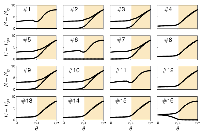
Figure S5: Topological degeneracy. In each of the sixteen sectors of the Wilson loops ($\#1\sim 16$), only the lowest two energy levels are displayed. KSL$\times$KSL phase: ninefold degeneracy ($\#1,2,3,5,6,7,9,10,11$). RVB phase: fourfold degeneracy ($\#1,6,11,16$). See Table SIII for details of the Wilson loop sectors.

We identify topological degeneracy by decomposing the ground state manifold to the sixteen sectors of the Wilson loop operators ($\#1\sim 16$). Figure S5 displays the lowest two energy levels in each of the sixteen sectors. In the KSL$\times$KSL phase, we identify ninefold degeneracy in the sectors of $\#1,2,3,5,6,7,9,10,11$. In the RVB phase, we find fourfold degeneracy in the sectors of $\#1,6,11,16$. See Table SIII for details of the sixteen Wilson loop sectors.

	$\mathcal{W}_{x}^{\sigma}$	$\mathcal{W}_{y}^{\sigma}$	$\mathcal{W}_{x}^{\tau}$	$\mathcal{W}_{y}^{\tau}$
#1	$-1$	$-1$	$-1$	$-1$
#2	$-1$	$-1$	$-1$	$+1$
#3	$-1$	$-1$	$+1$	$-1$
#4	$-1$	$-1$	$+1$	$+1$
#5	$-1$	$+1$	$-1$	$-1$
#6	$-1$	$+1$	$-1$	$+1$
#7	$-1$	$+1$	$+1$	$-1$
#8	$-1$	$+1$	$+1$	$+1$
#9	$+1$	$-1$	$-1$	$-1$
#10	$+1$	$-1$	$-1$	$+1$
#11	$+1$	$-1$	$+1$	$-1$
#12	$+1$	$-1$	$+1$	$+1$
#13	$+1$	$+1$	$-1$	$-1$
#14	$+1$	$+1$	$-1$	$+1$
#15	$+1$	$+1$	$+1$	$-1$
#16	$+1$	$+1$	$+1$	$+1$

Table SIII: Sixteen Wilson loop sectors of the ground state manifold. The sixteen sectors ($\#1\sim 16$) are characterized by the eigenvalues of the four Wilson loop operators, $(\mathcal{W}_{x}^{\sigma},\mathcal{W}_{y}^{\sigma},\mathcal{W}_{x}^{\tau},\mathcal{W}_{y}^{\tau})=(\pm 1,\pm 1,\pm 1,\pm 1)$.

VI Estimation of the critical exponent

In exact diagonalization studies, it is usually a challenging task to conduct a finite size scaling analysis and obtain critical exponents. It is because system sizes are restricted to 40$\sim$50 sites at the most due to the exponential growth of the Hilbert space. In fact, our 48-site bilayer cluster reaches almost the maximum system size allowed by currently available resources. Nevertheless, we attempt to extract a critical exponent from our 48-site ED results.

Figure S6 shows the estimations of the critical exponent $\beta$ from three quantities. We plot Figs. 3 and 4 of the main text in the domain of the parameter, $k\equiv K_{\sigma}/G$. The critical exponent $\beta$ is estimated by fitting the function $A(k_{c}-k)^{\beta}$ to each data. In this procedure, the location of the critical point is fixed by the value $k_{c}=\cos\theta_{c}/\sin\theta_{c}=0.94$ ($\theta_{c}=0.26\pi$). Although it is a rough estimation, the extracted values ($\beta=0.31,0.32$) are close to the critical exponent ($\beta_{\textup{3D-Ising}}=0.326$) of the 3D Ising universality class Ferrenberg et al. (2018). See Fig. S6(b,c).

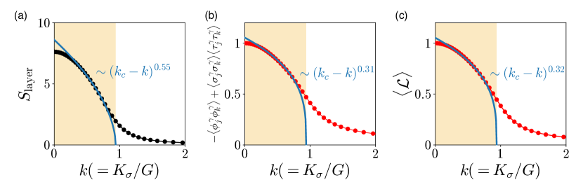
Figure S6: Extracting the critical exponent $\beta$ from three quantities. (a) The entanglement entropy $S_{\rm layer}$: $\beta=0.55$. (b) The spin-spin correlator $\langle\phi_{j}^{\gamma}\phi_{k}^{\gamma}\rangle-\langle\sigma_{j}^{\gamma}\sigma_{k}^{\gamma}\rangle\langle\tau_{j}^{\gamma}\tau_{k}^{\gamma}\rangle$: $\beta=0.31$. (c) The expectation value of the loop operator $\langle\mathcal{L}\rangle$: $\beta=0.32$.

References

Winkler (2003)Roland Winkler, Spin-orbit coupling
effects in two-dimensional electron and hole systems, Vol. 191 (Springer, 2003) —See Appendix B.
Nica et al. (2023)E. M. Nica, M. Akram,
A. Vijayvargia, R. Moessner, and O. Erten, “Kitaev spin-orbital bilayers and their
moiré superlattices,” npj Quantum Mater. 8, 9 (2023).
Ferrenberg et al. (2018)A. M. Ferrenberg, J. Xu, and D. P. Landau, “Pushing the limits of Monte
Carlo simulations for the three-dimensional Ising model,” Phys.
Rev. E 97, 043301
(2018).