Semi-Lagrangian Finite-Element Exterior Calculus for Incompressible Flows

Abstract

We develop a semi-Lagrangian discretization of the time-dependent incompressible Navier-Stokes equations with free boundary conditions on arbitrary simplicial meshes. We recast the equations as a non-linear transport problem for a momentum 1-form and discretize in space using methods from finite-element exterior calculus. Numerical experiments show that the linearly implicit fully discrete version of the scheme enjoys excellent stability properties in the vanishing viscosity limit and is applicable to inviscid incompressible Euler flows. We obtain second-order convergence and conservation of energy is achieved through a Lagrange multiplier.

1 Incompressible Navier-Stokes Equations

We consider the incompressible Navier-Stokes equations—a standard hydrodynamic model for the motion of an incompressible, potentially-viscous fluid—in a container with rigid walls, where we impose so-called “free boundary conditions” in the parlance of [31, p. 346] and [43, p. 502], see the latter article for further references. We search the fluid velocity field $\boldsymbol{u}(t,\boldsymbol{x})$ and the pressure $p(t,\boldsymbol{x})$ as functions of time $t$ and space $\boldsymbol{x}$ on a bounded, Lipschitz domain $\Omega\subset\mathbb{R}^{d}$ such that they solve the evolution boundary-value problem

$$\partial_{t}\boldsymbol{u}+\boldsymbol{u}\cdot\nabla\boldsymbol{u}-\epsilon\Delta\boldsymbol{u}+\nabla p =\boldsymbol{f}, \text{on }]0,T[\times\Omega,$$ (1a)

$$\nabla\cdot\boldsymbol{u} =0, \text{on }]0,T[\times\Omega,$$ (1b)

$$\boldsymbol{u}\cdot\boldsymbol{n} =0, \text{on }]0,T[\times\partial\Omega,$$ (1c)

$$\epsilon\boldsymbol{n}\times\nabla\times\boldsymbol{u} =\boldsymbol{0}, \text{on }]0,T[\times\partial\Omega,$$ (1d)

$$\boldsymbol{u} =\boldsymbol{u_{0}}, \text{on }\{0\}\times\Omega,$$ (1e)

where $\epsilon\geq 0$ denotes a (non-dimensional) viscosity, $\boldsymbol{f}$ a given source term, $T>0$ the final time, $\partial\Omega$ the boundary of $\Omega$, and $\boldsymbol{n}(\boldsymbol{x})$ the outward normal vector at $\boldsymbol{x}\in\partial\Omega$. The initial condition $\boldsymbol{u_{0}}$ is to satisfy $\nabla\cdot\boldsymbol{u_{0}}=0$ in $\Omega$ and $\boldsymbol{u_{0}}\cdot\boldsymbol{n}=0$, $\epsilon\boldsymbol{n}\times\nabla\times\boldsymbol{u_{0}}=\boldsymbol{0}$ on $\partial\Omega$. Based on the variational description of the Navier-Stokes equations as described in [4], $\boldsymbol{u}$ can be interpreted as a differential 1-form [33] and we can recast system (1) in the following way. Let $\Lambda^{k}(\Omega)$ for $k\in\mathbb{N}$ denote the space of differential $k$-forms on $\Omega$. Then we search $\omega\in\Lambda^{1}(\Omega)$ and $p\in\Lambda^{0}(\Omega)$ such that

$$D_{\boldsymbol{u}}\omega+\epsilon\delta\text{d}\omega+\text{d}p =f, \text{on }]0,T[\times\Omega,$$ (2a)

$$\delta\omega =0, \text{on }]0,T[\times\Omega,$$ (2b)

$$\operatorname{tr}\star\omega =0, \text{on }]0,T[\times\partial\Omega,$$ (2c)

$$\epsilon\operatorname{tr}\star\text{d}\omega =0, \text{on }]0,T[\times\partial\Omega,$$ (2d)

$$\omega =\omega_{0}, \text{on}\{0\}\times\Omega,$$ (2e)

where $D_{\boldsymbol{u}}\omega$ denotes the material derivative of $\omega$ with respect to $\boldsymbol{u}$, $\text{d}:\Lambda^{k-1}(\Omega)\mapsto\Lambda^{k}(\Omega)$ the exterior derivative, $\delta:\Lambda^{k}(\Omega)\mapsto\Lambda^{k-1}(\Omega)$ the exterior coderivative, and the trace $\operatorname{tr}$ is the pullback under the embedding $\partial\Omega\subset\bar{\Omega}$. Here, $\boldsymbol{u}$ is related to $\omega$ through $\omega\coloneqq\boldsymbol{u}^{\musFlat{}}$, i.e. $\boldsymbol{u}$ is the vector proxy of $\omega$ w.r.t. the Euclidean metric. Similarly, we have that $\Lambda^{1}(\Omega)\ni\omega_{0}\coloneqq\boldsymbol{u_{0}}^{\musFlat{}}$ and $\Lambda^{1}(\Omega)\ni f\coloneqq\boldsymbol{f}^{\musFlat{}}$. We would like to emphasize that $\omega$ does not represent the vorticity, but the 1-form representation of the velocity in this work. Note that (2) can be derived through classical vector calculus for vector proxies as shown in Appendix A for $d=3$.

As shown in [17, 18], sufficiently-smooth solutions $\omega:]0,T[\mapsto\Lambda^{1}(\Omega)$ of the incompressible Navier-Stokes equations as given in system (2) satisfy an energy relation, that is,

$$\frac{dE}{dt}(t)\coloneqq\frac{d}{dt}\frac{1}{2}\int_{\Omega}\omega(t)\wedge\star\omega(t)=-\epsilon\int_{\Omega}\text{d}\omega(t)\wedge\star\text{d}\omega(t)+\int f(t)\wedge\star\omega(t).$$ (3)

This relation implies energy conservation for $\epsilon=0$ and $f=0$. Note that the Onsager conjecture tells us that in the case $\epsilon=0$ the solutions need to be at least Hölder regular with exponent $\frac{1}{3}$ for energy conservation to hold [28].

Remark 1.

We acknowledge that the boundary condition (1d) is non-standard. This boundary condition was chosen because it is the natural boundary condition associated to system (2). At first glance, an intuitive method to enforce the standard no-slip boundary conditions is to replace (1d) by $\epsilon\boldsymbol{u}\times\boldsymbol{n}=\boldsymbol{0}$ on $]0,T[\times\partial\Omega$. To obtain well-posedness, it is then also required to impose $p=0$ on $]0,T[\times\partial\Omega$. However, in that case, we lose the natural boundary condition $\boldsymbol{u}\cdot\boldsymbol{n}=0$. Instead, $\epsilon\boldsymbol{u}\times\boldsymbol{n}=\boldsymbol{0}$ can be enforced using boundary penalty methods as will be shown in future work. In the case $\epsilon=0$, the only imposed boundary condition (1c) is standard.

Remark 2.

Boundary conditions (1c),(1d) can be interpreted as slip boundary conditions. However, on smooth domains $\Omega$, they are only equivalent to Navier’s slip boundary conditions if the Weingarten map related to $\partial\Omega$ vanishes [31, section 2].

2 Outline and Related Work

We propose a semi-Lagrangian approach to the discretization of the reformulated Navier-Stokes boundary value problem (2). This method revolves around the discretization of the material derivative $D_{\boldsymbol{u}}\omega$ in the framework of a finite-element Galerkin discretization on a fixed spatial mesh. The main idea is to approximate $D_{\boldsymbol{u}}\omega$ by backward difference quotients involving transported snapshots of the 1-form $\omega$, which can be computed via the pullback induced by the flow of the velocity vector field $\boldsymbol{u}$.

Semi-Lagrangian methods for transient transport equations like (2) are well-established for the linear case when $\boldsymbol{u}$ is a given Lipschitz-continuous velocity field. In particular, for $\omega$ a 0-form, that is, a plain scalar-valued function, plenty of semi-Lagrangian approaches have been proposed and investigated, see, for instance, [6, 7, 19, 21, 23, 35, 39, 40, 5, 8, 45]. We refer to [25, Chapter 5] for a comprehensive pre-2013 literature review on the analysis of general semi-Lagrangian schemes. Most of these methods focus on mapping point values under the flow, with the exception of a particularly interesting class of semi-Lagrangian methods known as Lagrange-Galerkin methods. Lagrange-Galerkin methods do not transport point values, but rather triangles (in 2D) or tetrahedra (in 3D). Refer to [10] for a review of those methods.

Meanwhile semi-Lagrangian methods for transport problems for differential forms of any order have been developed [26, 24, 25]. The next section will review these semi-Lagrangian methods for linear transport problems with emphasis on 1-forms. We will also introduce a new scheme which is second-order in space and time based on so-called “small edges”, see section 3.1.2 for details.

Semi-Lagrangian schemes for the incompressible Navier-Stokes equations are also well-documented in literature, with emphasis on the Lagrange-Galerkin method [10, 13, 14, 30, 20, 9, 11]. A survey of the application of Lagrange-Galerkin methods to the incompressible Navier-Stokes equations is given in [10]. It is important to note that these methods require the evaluation of integrals of transported quantities and, in case these integrals cannot be computed exactly, instabilities can occur [8, 32]. A possible remedy is to add an additional stabilization term that includes artificial diffusion [10]. Other semi-Lagrangian methods for incompressible Navier-Stokes equations directly transport point values with the nodes of a mesh instead of evaluating integrals of transported quantities, see [34, 29, 46, 47, 12] and [16], where the last work makes use of exponential integrators [15]. Most authors employ spectral elements for the discretization in space [34, 29], but any type of finite-element space with degrees-of-freedom relying on point evaluations can be used. The methods proposed in [46, 47] are also based on finite-element spaces with degrees-of-freedom on nodes, but employ backward-difference approximations for the material derivative. The work [12] proposes an explicit semi-Lagrangian method still built around the transport of point values in the nodes of the mesh. The diffusion term is also taken into account in a semi-Lagrangian fashion and the incompressibility constraint is enforced by means of a Chorin projection. Also [12] proposes an explicit semi-Lagrangian scheme using the same principles, but based on the vorticity-streamfunction form of the incompressible Navier-Stokes equations.

All the mentioned semi-Lagrangian schemes rely on the transport of point values of continuous vector fields, which is the perspective embraced in formulation (1). However, we believe that, in particular in the case of free boundary conditions (1c) and (1d), the semi-Lagrangian method based on (2) offers benefits similar to the benefits bestowed by the use of discrete differential forms (finite-element exterior calculus, FEEC [2, 3]) for the discretization of electromagnetic fields. Section 4 will convey that the boundary conditions (2c), (2d), and the incompressiblity constraint can very naturally be incorporated into a variational formulation of (2) posed in spaces of 1-forms. This has been the main motivation for pursuing the new idea of a semi-Lagrangian method for (2) that employs discrete 1-forms. Another motivation has been the expected excellent robustness of the semi-Lagrangian discretization in the limit $\epsilon\mapsto 0$. Numerical tests reported in section 5 will confirm this.

Two more aspects of our method are worth noting: Firstly, a discrete 1-form $\omega_{h}$ will not immediately spawn a continuous velocity field $\boldsymbol{u}_{h}=\omega_{h}^{\musFlat{}}$, However, continuity is essential for defining a meaningful flow. We need an additional averaging step, which we present in section 4.1. Secondly, since semi-Lagrangian methods fail to respect the decay/conservation law (3) exactly, we present a way how to enforce them in section 4.3.

3 Semi-Lagrangian Advection of differential forms

3.1 Discrete differential forms

(a) 9 small edges of a second-order element in 2D. All the edges between the different connection points are small edges. In 3D, we simply have all these small edges on the faces of the simplex.

edge no.	l.s.f.	edge no.	l.s.f.
$1$	$\left[\begin{smallmatrix}x\\ y\end{smallmatrix}\right]\mapsto\left[\begin{smallmatrix}y(x+y-1)\\ -(x-1)(x+y-1)\end{smallmatrix}\right]$	$6$	$\left[\begin{smallmatrix}x\\ y\end{smallmatrix}\right]\mapsto\left[\begin{smallmatrix}(y-1)(x+y-1)\\ x(1-x-y)\end{smallmatrix}\right]$
$2$	$\left[\begin{smallmatrix}x\\ y\end{smallmatrix}\right]\mapsto\left[\begin{smallmatrix}-y^{2}\\ y(x-1)\end{smallmatrix}\right]$	$7$	$\left[\begin{smallmatrix}x\\ y\end{smallmatrix}\right]\mapsto\left[\begin{smallmatrix}-xy\\ x(x-1)\end{smallmatrix}\right]$
$3$	$\left[\begin{smallmatrix}x\\ y\end{smallmatrix}\right]\mapsto\left[\begin{smallmatrix}-y^{2}\\ xy\end{smallmatrix}\right]$	$8$	$\left[\begin{smallmatrix}x\\ y\end{smallmatrix}\right]\mapsto\left[\begin{smallmatrix}y(1-y)\\ xy\end{smallmatrix}\right]$
$4$	$\left[\begin{smallmatrix}x\\ y\end{smallmatrix}\right]\mapsto\left[\begin{smallmatrix}-xy\\ x^{2}\end{smallmatrix}\right]$	$9$	$\left[\begin{smallmatrix}x\\ y\end{smallmatrix}\right]\mapsto\left[\begin{smallmatrix}y(x+y-1)\\ x(1-x-y)\end{smallmatrix}\right]$
$5$	$\left[\begin{smallmatrix}x\\ y\end{smallmatrix}\right]\mapsto\left[\begin{smallmatrix}x(1-y)\\ x^{2}\end{smallmatrix}\right]$

(b) Local shape functions (l.s.f.) for the unit triangle associated with second-order, discrete differential forms in 2D as proposed in [38]. Each shape function corresponds to the small edge in (a) with the same numbering.

Figure 1: Illustration of small edges (a) and corresponding local shape functions (b) for the unit triangle.

We start from a simplicial triangulation $\mathcal{K}_{h}(\Omega)$ of $\Omega$, which may rely on a piecewise linear approximation of $\partial\Omega$ so that it covers a slightly perturbed domain.

3.1.1 Lowest-order case: Whitney forms

For $\Lambda^{0}(\Omega)$—the space of 0-forms on $\Omega$, which is just a space of real-valued functions—the usual (Lagrange) finite-element space of continuous, piecewise-linear, polynomial functions provides the space $\Lambda^{0}_{h,1}(\Omega)$ of lowest-order discrete 0-forms.

Let $d\in\{2,3\}$, $K$ a $d$-simplex with edges $\{e_{1},..,e_{3(d-1)}\}$. To construct lowest-order discrete 1-forms on $K$, we associate to every edge $e_{i}$ a local shape function $w^{e_{i}}$. Let the edge $e_{i}$ be directed from vertex $v_{i}^{1}$ to $v_{i}^{2}$, then the local shape function $w^{e_{i}}\in\Lambda^{1}(K)$ associated with edge $e_{i}$ is

$$w^{e_{i}}\coloneqq\lambda_{\boldsymbol{v}^{1}_{i}}\text{d}\lambda_{\boldsymbol{v}^{2}_{i}}-\lambda_{\boldsymbol{v}^{2}_{i}}\text{d}\lambda_{\boldsymbol{v}^{1}_{i}},$$ (4)

where $\lambda_{\boldsymbol{v}}$ represents the barycentric coordinate associated with vertex $\boldsymbol{v}$. We define the lowest-order, local space of discrete 1-forms

$$\Lambda_{h,1}^{1}(K)\coloneqq\operatorname{span}\{w^{e};e\text{ an edge of }K\}.$$ (5)

Using these local spaces, we can define the global space of lowest-order, discrete 1-forms

$$\Lambda_{h,1}^{1}(\Omega)\coloneqq\{\omega\in\Lambda^{1}(\Omega);\forall K\in\mathcal{K}_{h}(\Omega):\omega|_{K}\in\Lambda_{h,1}^{1}(K)\},$$ (6)

where $\Lambda^{1}(\Omega)$ again denotes the space of differential 1-forms on $\Omega$. We demand that for every $\omega\in\Lambda^{1}(\Omega)$ integration along any smooth oriented path yields a unique value. Thus, the requirement $\omega\in\Lambda^{1}(\Omega)$ imposes tangential continuity on the vector proxy of $\omega$.

3.1.2 Second-order discrete forms

Similar to the lowest-order case, the space $\Lambda^{0}_{h,2}(\Omega)$ of second-order discrete 0-forms is spawned by the usual (Lagrange) finite-element space of continuous, piecewise-quadratic, polynomial functions.

Let $d\in\{2,3\}$, $K$ a $d$-simplex with edges $\{e_{1},..,e_{3(d-1)}\}$ and vertices $\{\boldsymbol{v}_{1},..,\boldsymbol{v}_{d+1}\}$. To construct second-order discrete 1-forms, we associate local shape functions to ”small edges”. We can construct $3(d+1)(d-1)$ small edges [38, Definition 3.2] by defining $\forall i\in\{1,..,d+1\}$ and $\forall j\in\{1,..,3(d-1)\}$

$$\{\boldsymbol{v}_{i},e_{j}\}\coloneqq\{\boldsymbol{v}_{i}+\frac{1}{2}(\boldsymbol{x}-\boldsymbol{v}_{i});\boldsymbol{x}\in e_{j}\},$$

where $\{\boldsymbol{v}_{i},e_{j}\}$ denotes the small edge. In Figure 1(a) we illustrate the 9 small edges of a 2-simplex. For example, we see that small edge 9 can be written as $\{(0,0),[(1,0),(0,1)]\}$. To make the difference between small edges and edges of the mesh explicit, we will sometimes refer to the latter as ”big edges”.

The local shape function [38, Definition 3.3] associated with $\{\boldsymbol{v}_{i},e_{j}\}$ is given by

$$w^{\{\boldsymbol{v}_{i},e_{j}\}}\coloneqq\lambda_{\boldsymbol{v}_{i}}w^{e_{j}},$$

where $w^{e_{j}}$ denotes the Whitney 1-form associated with the big edge $e_{j}$ as defined in (4). In Figure 1(b) we give explicit expressions for the shape functions associated with the small edges in Figure 1(a). Note that the local shape functions of the form $w^{\{\boldsymbol{v},e\}}$ associated with small edges in the interior ($d=2$) or on the same face ($d=3$) of the form $\{\boldsymbol{v},e\}$ such that $\boldsymbol{v}\notin\partial e$ (example: small edge 7, 8, and 9 in Figure 1(a)) are linearly dependent. We define the second-order, local space of discrete 1-forms [38, Definition 3.3]

$$\Lambda_{h,2}^{1}(K)\coloneqq\operatorname{span}\{w^{\{\boldsymbol{v},e\}};\boldsymbol{v}\text{ a vertex of }K,e\text{ a (big) edge of }K\}.$$ (7)

Using these local spaces, we can define the global space of second-order, discrete 1-forms

$$\Lambda_{h,2}^{1}(\Omega)\coloneqq\{\omega\in\Lambda^{1}(\Omega);\forall K\in\mathcal{K}_{h}(\Omega):\omega|_{K}\in\Lambda_{h,2}^{1}(K)\},$$ (8)

where again we have tangential continuity by a similar argument as in section 3.1.1.

3.1.3 Projection operators

We denote by $\mathcal{E}_{h,p}(\Omega)$ the global set of big edges ($p=1$) or small edges ($p=2$) associated with $\mathcal{K}_{h}(\Omega)$. We will define the projection operator $\mathcal{I}_{h,p}:\Lambda^{1}(\Omega)\mapsto\Lambda_{h,p}^{1}(\Omega)$ as the unique operator that maps $\omega\in\Lambda^{1}(\Omega)$ to $\omega_{h}\in\Lambda^{1}_{h,p}(\Omega)$ such that the mismatch

$$\sum_{e\in\mathcal{E}_{h,p}(\Omega)}\left(\int_{e}\omega-\int_{e}\omega_{h}\right)^{2}$$ (9)

is minimized. Note that for $p=1$, this mismatch can be made to vanish. In this case, $\mathcal{I}_{h,1}$ agrees with the usual edge-based nodal projection operator [27, Eq. (3.11)].

In practice, we can compute the projection locally as follows. Let $K\in\mathcal{K}_{h}(\Omega)$ be a $d$-simplex, $d\in\{2,3\}$, and let $\{s_{1},..,s_{N_{p,d}}\}$ and $\{w^{s_{1}},..,w^{s_{N_{p,d}}}\}$ denote the corresponding big ($p=1$) or small ($p=2$) edges and corresponding shape functions as introduced above. Specifically, we have $N_{1,2}=3$, $N_{1,3}=6$, $N_{2,2}=9$, and $N_{2,3}=24$. We can define the matrix

$$\left(\mathcal{M}\right)_{i,j}=\int_{s_{i}}w^{s_{j}},\hskip 28.45274pt1\leq i,j\leq N_{p,d}.$$ (10)

We will say that there is an interaction from edge $s_{j}$ to $s_{i}$ if $(\mathcal{M})_{i,j}\neq 0$. Note that for $p=1$, $\mathcal{M}$ is the identity matrix. For $p=2$ the local shape functions are linearly dependent and, thus, the above matrix is not invertible. However, we can decompose $\mathcal{M}$ into invertible and singular sub-matrices. For illustrative purposes we display for $p=2$ and $d=2$ the decomposition of $\mathcal{M}$ in Figure 2(b). The three top-left sub-matrices in Figure 2(b) are invertible $2\times 2$ matrices that describe the interaction between the two small edges that lie on the same big edge, that is, the blue, red, and green submatrix in Figure 2(b) correspond to the blue, red, and green small edges in Figure 2(a), respectively. The orange submatrix in Figure 2(b) is a $3\times 3$ matrix with rank 2 that describes the interaction between the three small edges that lie in the interior of the simplex in Figure 2(a), that is, the orange small edges. The gray submatrix encodes the one-directional interaction from the the small edges that lie on a big edge to the small edges in the interior. Note that the decomposition of $\mathcal{M}$ as given in Figure 2(b) is not limited to $d=2$. The idea can be extended to $d=3$ by considering each face of a 3-simplex as a 2-simplex. This is sufficient, since for $d=3$ we have no small edges in the interior and there is no interaction between small edges that do not lie on the same face. We give the general structure of $\mathcal{M}$ in Figure 2(c). Note that the small, purple sub-matrices represent invertible $2\times 2$ matrices and the bigger, orange sub-matrices represent $3\times 3$ matrices with rank 2.

(a) 2-simplex $K$

(b) matrix $\mathcal{M}$ ($d=2$)

(c) matrix $\mathcal{M}$ ($d=3$)

Figure 2: For $p=2$ and $d=2$ the matrix $\mathcal{M}$ corresponding to the 2-simplex $K$ in (a) has the form given in (b). Each row and column in $\mathcal{M}$ is associated to a small edge in (a). Each submatrix in (b) describes the interactions between edges with the same color in (a). The gray submatrix is an exception as it describes the one-directional interaction between the small edges that lie on a big edge and the small edges that lie in the interior. For $d=3$, $\mathcal{M}$ has the structure as shown in Figure 2(c), where the purple submatrices are $2\times 2$ invertible matrices and the orange submatrices are $3\times 3$ matrices of rank 2.

In order to find $\omega_{h}\big{|}_{K}\in\Lambda^{1}_{h,p}(K)$ such that $\omega_{h}\big{|}_{K}=\mathcal{I}_{h,p}\omega\big{|}_{K}$, let $\vec{\eta}_{K}$ be a vector of coefficients $\eta^{1}_{K},..,\eta_{K}^{N_{p,d}}$ such that

$$\left.\omega_{h}\right|_{K}=\sum_{i=1}^{N_{p,d}}\eta^{i}_{K}w^{s_{i}}.$$ (11)

We can then compute $\vec{\eta}_{K}$ as a least-squares solution of

$$\mathcal{M}\vec{\eta}_{K}=\left(\int_{s_{i}}\omega\right)_{1\leq i\leq N_{p,d}}.$$ (12)

Without loss of generality we assume that $\mathcal{M}$ has the form as given in Figure 2(c). Then, we solve (12) as follows:

1. The local shape functions related to small edges that lie on a big edge of the simplex are linearly independent. We solve for their coefficients first, that is, we solve the system corresponding to the invertible blue sub-matrices in Figure 2(c) first.

2. Using the results from step 1, we can move the gray submatrix in Figure 2(c) to the right-hand side. Then, we solve the matrix-system corresponding to the orange sub-matrices in Figure 2(c) in a least-squares sense.

If we perform the above steps for all $K\in\mathcal{K}_{h}(\Omega)$, we find $\omega_{h}=\mathcal{I}_{h,p}\omega\in\Lambda^{1}_{h,p}(\Omega)$. Note that only the shape functions associated to small edges on a face contribute to the tangential fields on that face. Therefore, the above procedure yields tangential continuity.

Remark 3.

For $p=1$, (12) reduces to

$$\eta^{i}_{K}=\int_{s_{i}}\omega,\hskip 28.45274pt\forall i\in\{1,..,3(d-1)\}$$ (13)

with $s_{i}$ a big edge of the $d$-simplex $K$ for all $i\in\{1,..,3(d-1)\}$. This yields the standard nodal interpolation operator of [27, Eq. (3.11)].

3.2 Semi-Lagrangian material derivative

The method described in this section is largely based on [25, 26]. Throughout this section, unless stated otherwise, we fix the stationary, Lipschitz-continuous velocity field $\boldsymbol{u}\in W^{1,\infty}(\Omega)$ with $\boldsymbol{u}\cdot\boldsymbol{n}=\boldsymbol{0}$ on $\partial\Omega$. This means that we consider a linear transport problem and our main concern will be the discretization of the material derivative $D_{\boldsymbol{u}}\omega$ for a 1-form $\omega$. We can define the flow $]0,T[\times\Omega\ni(\tau,\boldsymbol{x})\mapsto X_{\tau}(\boldsymbol{x})\in\mathbb{R}^{d}$ as the solution of the initial value problems

$$\frac{\partial}{\partial\tau}X_{t,t+\tau}(\boldsymbol{x})=\boldsymbol{u}(X_{t,t+\tau}(\boldsymbol{x})),\hskip 28.45274ptX_{t}(\boldsymbol{x})=\boldsymbol{x}.$$ (14)

Given that flow we can define the material derivative for a time-dependent differential 1-form $\omega$

$$D_{\boldsymbol{u}}\omega(t)\coloneqq\left.\frac{\partial}{\partial\tau}X_{t,t+\tau}^{*}\omega(t+\tau)\right|_{\tau=0}.$$ (15)

We employ a first- or second-order, backward-difference method to approximate the derivative. Writing $X_{t,t-\tau}^{*}$ for the pullback of forms under the flow, we obtain for sufficiently-smooth $t\mapsto\omega(t)$ and a timestep $0<\tau\rightarrow 0$

$$D_{\boldsymbol{u}}\omega(t) =\frac{1}{\tau}\left[\omega(t)-X_{t,t-\tau}^{*}\omega(t-\tau)\right]+\mathcal{O}(\tau^{2})$$ (16)

or

$$D_{\boldsymbol{u}}\omega(t) =\frac{1}{2\tau}\left[3\omega(t)-4X_{t,t-\tau}^{*}\omega(t-\tau)+X_{t,t-2\tau}^{*}\omega(t-2\tau)\right]+\mathcal{O}(\tau^{3}),$$ (17)

respectively. Note that both backward-difference methods are A-stable [41]. In the remainder of this section we restrict ourselves to (16), but exactly the same considerations apply to (17).

Given a temporal mesh $..<t^{n}<t^{n+1}<..$, we approximate $\omega(t^{n},\cdot)\in\Lambda^{1}(\Omega)$ by a discrete differential form $\omega_{h}^{n}\in\Lambda^{1}_{h,p}(\Omega)$ with $p\in\{1,2\}$. Using the backward-difference quotient (16), we can define the discrete material derivative for fixed timestep $\tau>0$

$$(D_{\boldsymbol{\beta}}\omega)(t^{n})\approx\frac{1}{\tau}\left[\omega_{h}^{n}-\mathcal{I}_{h,p}X_{t,t-\tau}^{*}\omega_{h}^{n-1}\right]\in\Lambda^{1}_{h,p}(\Omega),$$ (18)

where we need to use the projection operator $\mathcal{I}_{h,p}:\Lambda^{1}(\Omega)\mapsto\Lambda_{h,p}(\Omega)$ since $X_{t,t-\tau}^{*}\omega^{n-1}_{h}\notin\Lambda^{1}_{h,p}(\Omega)$ in general. Recall from section 3.1 that the degrees of freedom for discrete 1-forms are associated to small ($p=2$) or big ($p=1$) edges. As discussed in section 3.1.3, evaluating the interpolation operator entails integrating $X_{t,t-\tau}^{*}\omega^{n-1}_{h}$ over small ($p=2$) or big ($p=1$) edges. We can approximate these integrals as follows

$$\int_{e}X_{t,t-\tau}^{*}\omega_{h}^{n-1}=\int_{X_{t,t-\tau}(e)}\omega_{h}^{n-1}\approx\int_{\bar{X}_{t,t-\tau}(e)}\omega_{h}^{n-1},$$ (19)

where $e$ is a small or big edge and

$$\bar{X}_{t,t-\tau}(e)=\left\{(1-\xi)X_{t,t-\tau}(\boldsymbol{v}^{1})+\xi X_{t,t-\tau}(\boldsymbol{v}^{2});0\leq\xi\leq 1\right\}$$ (20)

with $\boldsymbol{v}^{1},\boldsymbol{v}^{2}$ the vertices of $e$. Instead of transporting the edge $e$ using the exact flow $X_{t,t-\tau}$, we follow [8, 25, 26] and only transport the vertices of the small edges ($p=2$) or big edges ($p=1$) and obtain a piecewise linear (second-order) approximation $\bar{X}_{t,t-\tau}(e)$ of the transported edge $X_{t,t-\tau}(e)$ as illustrated in Figure 3. We can approximate the movement of the endpoints of $e$ under the flow as defined by (14) by solving (14) using the explicit Euler method or Heun’s method for the first- and second-order case, respectively. We will elaborate on this further in section 4.1.

Figure 3: Edge $e$ (in red) is transported using the flow $\boldsymbol{\beta}$ (in blue). The exact transported edge $X_{\tau}(e)$ and the approximate transported edge $\bar{X}_{\tau}(e)$ are given in orange and green.

Algorithm 1 Splitting 1-simplex over mesh elements (see Figure 4 for illustration). Here, $K_{\text{ref}}$ denotes the reference simplex.

1:$x_{0}\in K_{0}\in\mathcal{K}_{h}(\Omega)$ and $x_{1}$ vertices of a 1-simplex $e$.

2:Number of elements $N$, elements $\{K_{0},..,K_{N-1}\}\in\mathcal{K}_{h}(\Omega)^{N}$.

3:$K\leftarrow K_{0}$

4:$F_{\text{old}}\leftarrow$ NULL

5:$K_{\text{old}}\leftarrow$ NULL

6:$N\leftarrow 1$

7:$E\leftarrow\{K\}$

8:while $x_{1}\notin K$ do

9:     Find the isoparametric mapping $\phi_{K}:K_{\text{ref}}\mapsto K$

10:     Find face $F\subset\partial K$ s.t. $F\neq F_{\text{old}}$ and $\phi_{K}^{-1}(e)\cap\phi_{K}^{-1}(F)\neq\emptyset$

11:     $K\leftarrow K\in\mathcal{K}_{h}(\Omega)$ s.t. $F\subset\partial K$ and $K\neq K_{\text{old}}$ ($K$ on the other side of face $F$)

12:     $F_{\text{old}}\leftarrow F$

13:     $N\leftarrow N+1$

14:     $E\leftarrow E\cup\{K\}$

15:end while

\begin{overpic}[width=433.62pt]{splitlineinelements.pdf} \put(25.0,35.0){\large$\phi_{K}:K_{\text{ref}}\mapsto K$} \put(64.0,27.0){$x_{0}$} \put(71.0,29.0){$e$} \put(66.0,30.0){$K$} \put(16.0,20.0){$\phi_{K}^{-1}(e)$} \put(12.5,26.0){$K_{\text{ref}}$} \put(63.0,21.0){$K_{0}$} \put(84.0,35.0){$x_{1}$} \par\end{overpic}

Figure 4: The red line indicates the line that spans multiple elements. On the left we see the reference triangle associated with the yellow element in the mesh on the right.

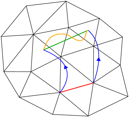
In Figure 3, we can also see that the approximate transported edge may intersect several different elements of the mesh. When we evaluate the integral in (19), it can happen that there are discontinuities of $\omega_{h}^{n-1}$ along $\bar{X}_{t,t-\tau}(e)$. Therefore, we cannot apply a global quadrature rule to the entire integral. Instead, we split $\bar{X}_{t,t-\tau}(e)$ into several segments defined by the intersection of $\bar{X}_{t,t-\tau}(e)$ with cells of the mesh. In our implementation, for the sake of stability, we find the intersection points by transforming back to a reference element as visualised in Figure 4. Algorithm 1 gives all details. Note that we can forgo the treament of any special cases (e.g. intersection with vertices) without jeopardizing stability. After we split the transported edge into segments, we can evaluate the integrals over these individual pieces exactly, because we know that $\omega_{h}^{n-1}$ is of polynomial form when restricted to individual elements of the mesh (see section 3.1).

When simulating the fluid model (2), we will not have access to an exact velocity field. Instead we only have access to an approximation of the velocity field. This approximation may not satisfy exact vanishing normal boundary conditions. Therefore, a part of $\bar{X}_{t,t-\tau}(e)$ may end up outside the domain. This can also happen due to an approximation of the flow by explicit timestepping. Since $\omega_{h}^{n-1}$ is not defined outside the domain, we set

$$\int_{\left.\bar{X}_{t,t-\tau}(e)\right|_{\mathbb{R}^{d}\setminus\Omega}}\omega_{h}^{n-1}\coloneqq\frac{\text{len}\bigg{(}\left.\bar{X}_{t,t-\tau}(e)\right|_{\mathbb{R}^{d}\setminus\Omega}\bigg{)}}{\text{len}\bigg{(}\bar{X}_{t,t-\tau}(e)\bigg{)}}\int_{e}\omega_{h}^{n-1},$$ (21)

where $\left.\bar{X}_{t,t-\tau}(e)\right|_{\mathbb{R}^{d}\setminus\Omega}$ is the part of $\bar{X}_{t,t-\tau}(e)$ that lies outside the domain $\Omega$ and $\text{len}\big{(}\cdot)$ gives the arclength of the argument. This is motivated by the situation displayed in Figure 5—a case where an edge gets transported out of the domain due to the use of approximate flow maps despite vanishing normal components of the velocity. If we set the value defined in (21) to zero in this case, it would be equivalent to applying vanishing tangential boundary conditions, which is inconsistent with (1). Instead, (21) just takes the tangential components from the previous timestep.

We arrive at the following approximation of the material derivative

$$(D_{\boldsymbol{\beta}}\omega)(t^{n})\approx\frac{1}{\tau}\left[\omega_{h}^{n}-\mathcal{I}_{h,p}\bar{X}_{t,t-\tau}^{*}\omega_{h}^{n-1}\right],$$ (22)

where the only difference between (18) and (22) is that $X_{t,t-\tau}$ was replaced by $\bar{X}_{t,t-\tau}$ and $\mathcal{I}_{h,p}$ is implemented based on (21). Note that in our scheme $\bar{X}_{t,t-\tau}^{*}$ is always evaluated in conjunction with $\mathcal{I}_{h,p}$, which means that we need define $\bar{X}_{t,t-\tau}$ only on small ($p=2$) or big ($p=1$) edges. In fact, $\bar{X}_{t,t-\tau}$ is defined through (20) for all points that lie on small ($p=2$) or big ($p=1$) edges.

Figure 5: A coarse triangulation of $\Omega=\{\boldsymbol{x}\in\mathbb{R}^{2};||x||<1\}$ with the velocity field $\boldsymbol{u}=[-y,x]^{T}$ satisfying $\boldsymbol{u}\cdot\boldsymbol{n}=0$. Despite the vanishing normal components of the velocity, the blue edge gets transported out of the domain to the green edge.

Given a velocity field $\boldsymbol{u}\in W^{1,\infty}(\Omega)$ with $\boldsymbol{u}\cdot\boldsymbol{n}=\boldsymbol{0}$, it was shown in [26, section 4] that using a first-order backward difference scheme and lowest-order elements for the spatial discretization, we can approximate a smooth solution $\omega\in\Lambda^{1}(\Omega)$ of

$$D_{\boldsymbol{u}}\omega=0,$$ (23)

with an $L^{2}$-error of $\mathcal{O}(\tau^{-\frac{1}{2}}h)$, where $h$ is the spatial meshwidth and $\tau>0$ is the timestep size. However, numerical experiments [26, section 6] performed with $\tau=\mathcal{O}(h)$ show an error of $\mathcal{O}(h)$—a slight improvement over the a-priori estimates. This motivates us to link the timestep to the mesh width as $\tau=\mathcal{O}(h)$.

4 Semi-Lagrangian Advection applied to the Incompressible Navier-Stokes Equations

Given a temporal mesh $t_{0}<t_{1}<...<t_{N-1}<t_{N}$, we elaborate a single timestep $t_{n-1}\mapsto t_{n}$ of size $\tau\coloneqq t_{n}-t_{n-1}$, $n\leq N$. We assume that approximations $\omega^{k}_{h}\in\Lambda^{1}_{h,p}(\Omega)$ of $\omega(t_{k},\cdot)\in\Lambda^{1}(\Omega)$ are available for $k<n$ with $[0,T]\mapsto\omega\in\Lambda^{1}(\Omega)$ a solution of (2).

4.1 Approximation of the flow map

In the Navier-Stokes equations, the flow is induced by the unknown, time-dependent velocity field $\boldsymbol{u}(t,\boldsymbol{x})$. Therefore, (14) becomes

$$\frac{\partial}{\partial\tau}X_{t,t+\tau}(\boldsymbol{x})=\boldsymbol{u}(t+\tau,X_{t,t+\tau}(\boldsymbol{x})),\hskip 28.45274ptX_{t}(\boldsymbol{x})=\boldsymbol{x}\;,\quad t\in(0,T).$$ (24)

The discretization of the material derivative requires us to approximate the flow map $X_{t,t-\tau}$ in order to evaluate (20).

4.1.1 A first-order scheme

We use the explicit Euler method to approximate the (backward) flow according to

$$X_{t_{n},t_{n}-\tau}(\boldsymbol{x})\approx\boldsymbol{x}-\tau\boldsymbol{u}(t_{n}-\tau,\boldsymbol{x}),$$ (25)

where $t_{n}$ is a node in the temporal mesh and $\tau$ denotes the timestep size. We only have access to an approximation $\boldsymbol{u}_{h}^{n-1}\coloneqq(\omega^{n-1}_{h})^{\musSharp{}}$ of $\boldsymbol{u}$ at time $t_{n-1}$, which gives

$$X_{t_{n},t_{n}-\tau}(\boldsymbol{x})\approx\boldsymbol{x}-\tau\boldsymbol{u}_{h}^{n-1}(\boldsymbol{x}).$$ (26)

Note that a direct application of the explicit Euler method would require an evaluation of the velocity field at $t_{n}$. Instead, we perform a constant extrapolation and evaluate the velocity field at $t_{n-1}$, that is, we use $\boldsymbol{u}_{h}^{n-1}$ in (26).

The approximation $\boldsymbol{u}_{h}^{n-1}$ resides in the space of vector proxies for discrete differential 1-forms as discussed in section 3.1. This means that only tangential continuity of $\boldsymbol{u}_{h}^{n-1}$ across faces of elements of the mesh is guaranteed, while discontinuities may appear in the normal direction of the faces. Therefore, $\boldsymbol{u}_{h}^{n-1}$ is not defined point-wise—even though (26) requires point-wise evaluation. For that reason, we will replace $\boldsymbol{u}_{h}^{n-1}$ by a globally-continuous, smoothened velocity field $\bar{\boldsymbol{u}}_{h}^{n-1}$ that approximates $\boldsymbol{u}_{h}^{n-1}$ (see section 4.1.3 for the construction). We then have

$$X_{t_{n},t_{n}-\tau}(\boldsymbol{x})\approx\boldsymbol{x}-\tau\bar{\boldsymbol{u}}_{h}^{n-1}(\boldsymbol{x})$$ (27)

which yields a first-order-in-time approximation of $X_{t_{n},t_{n}-\tau}(\boldsymbol{x})$, provided that $\bar{\boldsymbol{u}}_{h}^{n-1}$ is a first-order approximation of $\boldsymbol{u}(t_{n-1},\cdot)$.

4.1.2 A second-order scheme

A second-order approximation can be achieved by using Heun’s method [44] instead of explicit Euler. We find the following second-order in time approximations

$$X_{t_{n},t_{n}-\tau}(\boldsymbol{x}) \approx\boldsymbol{x}-\frac{\tau}{2}\left[\boldsymbol{u}_{h}^{*}(\boldsymbol{x})+\boldsymbol{u}_{h}^{n-1}(\boldsymbol{x}-\tau\boldsymbol{u}_{h}^{*}(\boldsymbol{x}))\right],$$ (28)

$$X_{t_{n}t_{n}-2\tau}(\boldsymbol{x}) \approx\boldsymbol{x}-\tau\left[\boldsymbol{u}_{h}^{*}(\boldsymbol{x})+\boldsymbol{u}_{h}^{n-2}(\boldsymbol{x}-2\tau\boldsymbol{u}_{h}^{*}(\boldsymbol{x}))\right],$$ (29)

where we approximate the velocity field at $t_{n}$ by the linear extrapolation $\boldsymbol{u}_{h}^{*}=2\boldsymbol{u}_{h}^{n-1}-\boldsymbol{u}_{h}^{n-2}$. As described in section 4.1.1, we replace the velocity fields by suitable smooth approximations. We obtain

$$X_{t_{n},t_{n}-\tau}(\boldsymbol{x})\approx\bar{X}_{t-\tau}(\boldsymbol{x}) \coloneqq\boldsymbol{x}-\frac{\tau}{2}\left[\bar{\boldsymbol{u}}_{h}^{*}(\boldsymbol{x})+\bar{\boldsymbol{u}}_{h}^{n-1}(\boldsymbol{x}-\tau\bar{\boldsymbol{u}}_{h}^{*}(\boldsymbol{x}))\right],$$ (30)

$$X_{t_{n},t_{n}-2\tau}(\boldsymbol{x})\approx\bar{X}_{t-2\tau}(\boldsymbol{x}) \coloneqq\boldsymbol{x}-\tau\left[\bar{\boldsymbol{u}}_{h}^{*}(\boldsymbol{x})+\bar{\boldsymbol{u}}_{h}^{n-2}(\boldsymbol{x}-2\tau\bar{\boldsymbol{u}}_{h}^{*}(\boldsymbol{x}))\right],$$ (31)

where $\bar{\boldsymbol{u}}_{h}^{\bullet}$ with $\bullet=*,n-1,n-2$ denotes the smoothened version of $\boldsymbol{u}_{h}^{\bullet}$ as it will be constructed in the next section.

4.1.3 Smooth reconstruction of the velocity field

Given a discrete velocity field $\boldsymbol{u}_{h}^{\musFlat{}}\in\Lambda_{h,p}^{1}(\Omega)$, we can define a smoothened version $\bar{\boldsymbol{u}}_{h}$ of $\boldsymbol{u}_{h}$ that is

• Lipschitz continuous to ensure stable evaluation of (27),

• well-defined on every point of the meshed domain,

• practically computable, and

• second-order accurate.

We introduce $\bar{\boldsymbol{u}}_{h}$ as follows. Let $h_{\min}$ denote the length of the shortest edge of the mesh and $(u_{h}^{i})_{i=1,..,d}$ the components of $\boldsymbol{u}_{h}$. Then,

$$\bar{u}_{h}^{i}(\boldsymbol{x})=\frac{1}{h_{\min}}\int_{x_{i}-\frac{1}{2}h_{\min}}^{x_{i}+\frac{1}{2}h_{\min}}u^{i}_{h}([x_{1},\ldots,x_{i-1},\xi,x_{i+1},\ldots,x_{d}]^{T})d\xi$$ (32)

provides a second-order, Lipschitz-continuous approximation of $\boldsymbol{u}_{h}$. In the above definition, we can also replace $h_{\text{min}}$ by a localized parameter that scales as $\mathcal{O}(h)$ with $h$ the length of the edges ”close” to $\boldsymbol{x}$. Note that the above integral can be evaluated up to machine precision using the algorithm as described in section 3.2 for (19). The averaging (32) provides a second-order approximation of $\boldsymbol{u}_{h}$ on every point in the mesh.

4.2 A first- and second-order SL scheme

We are now ready to turn the ideas of section 3 into a concrete numerical scheme for the incompressible Navier-Stokes equations as given in (2). We cast (2a) and (2b) into weak form and, subsequently, do Galerkin discretization in space relying on those spaces of discrete differential forms introduced in section 3.1. For the first-order scheme, we have the following discrete variational formulation. Given $\omega^{n-1}_{h}\in\Lambda^{1}_{h,1}(\Omega)$, we search $p^{n}_{h}\in\Lambda^{0}_{h,1}(\Omega),\omega^{n}_{h}\in\Lambda^{1}_{h,1}(\Omega)$ such that

$$\left(\frac{1}{\tau}\left[\omega^{n}_{h}-\mathcal{I}_{h,1}\bar{X}_{t_{n},t_{n}-\tau}^{*}{\omega}^{n-1}_{h}\right],\eta_{h}\right)_{\Omega}$$

$$+\epsilon\left(\text{d}{\omega}^{n}_{h},\text{d}\eta_{h}\right)_{\Omega}+\left(\text{d}p^{n}_{h},\eta_{h}\right)_{\Omega} =\left(f^{n},\eta_{h}\right)_{\Omega},$$ (33a)

$$\left(\omega^{n}_{h},\text{d}\psi_{h}\right)_{\Omega} =0$$ (33b)

for all $\eta_{h}\in\Lambda^{1}_{h,1}(\Omega)$ and $\psi_{h}\in\Lambda^{0}_{h,1}(\Omega)$. $\mathcal{I}_{h,p}$ denotes the projection operator as defined in section 3.1. For the second-order scheme, we use second-order timestepping and second-order discrete differential forms. Given ${\omega}^{n-2}_{h},{\omega}^{n-1}_{h}\in\Lambda^{1}_{h,2}(\Omega)$, we search $p^{n}_{h}\in\Lambda^{0}_{h,2}(\Omega),{\omega}^{n}_{h}\in\Lambda^{1}_{h,2}(\Omega)$ such that

$$\bigg{(}\frac{1}{2\tau}\Big{[}3{\omega}^{n}_{h}-4\mathcal{I}_{h,2}\bar{X}_{t_{n},t_{n}-\tau}^{*}{\omega}^{n-1}_{h}+\mathcal{I}_{h,2}\bar{X}_{t_{n},t_{n}-2\tau}^{*}{\omega}^{n-2}_{h}\Big{]},\eta_{h}\bigg{)}_{\Omega}$$

$$+\epsilon\left(\text{d}{\omega}^{n}_{h},\text{d}\eta_{h}\right)_{\Omega}+\left(\text{d}p^{n}_{h},\eta_{h}\right)_{\Omega} =\left(f^{n},\eta_{h}\right)_{\Omega},$$ (34a)

$$\left(\omega^{n}_{h},\text{d}\psi_{h}\right)_{\Omega} =0$$ (34b)

for all $\eta_{h}\in\Lambda^{1}_{h,2}(\Omega)$ and $\psi_{h}\in\Lambda^{0}_{h,2}(\Omega)$. Numerical experiments reported in section 5 give evidence that these schemes indeed do provide first- and second-order convergence for smooth solutions. Note that the schemes presented in this section only require solving symmetric, linear systems of equations at every time-step.

4.3 Conservative SL schemes

In order to enforce energy-tracking—the correct behavior of the total energy $E(t)$ over time as expressed in (3)—we add a suitable constraint plus a Lagrange multiplier to the discrete variational problems proposed in section 4.2. Given ${\omega}^{n-1}_{h}\in\Lambda^{1}_{h,1}(\Omega)$, we search $p^{n}_{h}\in\Lambda^{0}_{h,1}(\Omega)$, ${\omega}^{n}_{h}\in\Lambda^{1}_{h,1}(\Omega)$, and $\mu^{n}\in\mathbb{R}$ such that

$$\left(\frac{1}{\tau}\left[{\omega}^{n}_{h}-\mathcal{I}_{h,1}\bar{X}_{t_{n},t_{n}-\tau}^{*}{\omega}^{n-1}_{h}\right],\eta_{h}\right)_{\Omega}+\left(\text{d}p^{n}_{h},\eta_{h}\right)_{\Omega}+\epsilon(\text{d}{\omega}^{n}_{h}, \text{d}\eta_{h})_{\Omega}$$

$$+\mu^{n}\left[(\omega^{n}_{h},\eta_{h})_{\Omega}+2\epsilon\tau(\text{d}\omega^{n}_{h},\text{d}\eta_{h})_{\Omega}-\tau(f^{n},\eta_{h})_{\Omega}\right] =\left(f^{n},\eta_{h}\right)_{\Omega},$$ (35a)

$$\left(\omega^{n}_{h},\text{d}\psi_{h}\right)_{\Omega} =0,$$ (35b)

$$\left(\omega^{n}_{h},\omega^{n}_{h}\right)_{\Omega}+2\epsilon\tau(\text{d}\omega^{n}_{h},\text{d}\omega^{n}_{h})_{\Omega}-\tau(f^{n},\omega^{n}_{h})_{\Omega} =\left(\omega^{n-1}_{h},\omega^{n-1}_{h}\right)_{\Omega}$$ (35c)

for all $\eta_{h}\in\Lambda^{1}_{h,1}(\Omega)$ and $\psi_{h}\in\Lambda^{0}_{h,1}(\Omega)$. Note that the last scalar equation enforces energy conservation for $\epsilon=0$ and $f=0$. To solve the nonlinear system (35) for $\omega^{n}_{h},p^{n}_{h},\mu^{n}$, we propose the following iterative scheme. Assume that we have a sequence $(\omega^{n}_{h,k})_{k\in\mathbb{N}}$ with $\omega^{n}_{h,k}\rightarrow\omega^{n}_{h}(k\rightarrow\infty)$. Then we can employ the Newton-like linearization

$$( \omega^{n}_{h},\omega^{n}_{h})_{\Omega}\leftarrow\left(\omega^{n}_{h,k},\omega^{n}_{h,k}\right)_{\Omega}$$

$$=\left(\omega_{h,k-1}^{n},\omega_{h,k-1}^{n}\right)_{\Omega}+2\left(\omega_{h,k-1}^{n},\omega^{n}_{h,k}-\omega^{n}_{h,k-1}\right)_{\Omega}+\mathcal{O}\left(||\omega^{n}_{h,k}-\omega^{n}_{h,k-1}||^{2}_{\Omega}\right).$$ (36)

We use the above expansion to replace the quadratic terms $\left(\omega^{n},\omega^{n}\right)_{\Omega}$ and $\left(\text{d}\omega^{n},\text{d}\omega^{n}\right)_{\Omega}$ and arrive at the following linear variational problem to be solved in every step of the inner iteration. Given ${\omega}_{h}^{n-1},{\omega}^{n}_{h,k-1}\in\Lambda^{1}_{h,1}(\Omega)$, we search $p^{n}_{h,k}\in\Lambda^{0}_{h,1}(\Omega)$, ${\omega}^{n}_{h,k}\in\Lambda^{1}_{h,1}(\Omega)$, and $\mu^{n}_{k}\in\mathbb{R}$ such that

$$\left(\frac{1}{\tau}\left[{\omega}^{n}_{h,k}-\mathcal{I}_{h,1}\bar{X}_{t_{n},t_{n}-\tau}^{*}{\omega}_{h}^{n-1}\right],\eta_{h}\right)_{\Omega}+\left(\text{d}p^{n}_{h,k},\eta_{h}\right)_{\Omega}+\epsilon( \text{d}{\omega}^{n}_{h,k},\text{d}\eta_{h})_{\Omega}$$

$$+\mu^{n}_{k}\left[(\omega^{n}_{h,k-1},\eta_{h})_{\Omega}+2\epsilon\tau(\text{d}\omega^{n}_{h,k-1},\text{d}\eta_{h})_{\Omega}-\tau(f^{n},\eta_{h})_{\Omega}\right] =\left(f^{n},\eta_{h}\right)_{\Omega},$$ (37a)

$$\left(\omega^{n}_{h,k},\text{d}\psi_{h}\right)_{\Omega} =0,$$ (37b)

$$\left(\omega_{h,k-1}^{n},\omega_{h,k-1}^{n}\right)_{\Omega}+2\left(\omega_{h,k-1}^{n},\omega^{n}_{h,k}-\omega^{n}_{h,k-1}\right)$$

$$+2\epsilon\tau[(\text{d}\omega_{h,k-1}^{n},\text{d}\omega_{h,k-1}^{n})_{\Omega}+2(\text{d}\omega_{h,k-1}^{n},\text{d}\omega^{n}_{h,k}-\text{d}\omega^{n}_{h,k-1})]$$

$$-\tau(f^{n},\omega^{n}_{h,k-1})_{\Omega} =\left(\omega^{n-1}_{h},\omega^{n-1}_{h}\right)_{\Omega}$$ (37c)

for all $\eta_{h}\in\Lambda^{1}_{h,1}(\Omega)$ and $\psi_{h}\in\Lambda^{0}_{h,1}(\Omega)$. This is a symmetric, linear system that is equivalent to the original system in the limit $(\omega^{n}_{h,k},p^{n}_{h,k},\mu^{n}_{k})\rightarrow(\omega^{n}_{h},p^{n}_{h},\mu^{n})$. In numerical experiments we observe that it takes around 2-3 steps of the inner iteration to converge to machine precision using an initial guess $\omega^{n}_{h,0}=\omega^{n-1}_{h}$. We can apply the same idea for energy-tracking to our second-order scheme as proposed in section 4.2.

5 Numerical Results

In this section, we present multiple numerical experiments to validate the new scheme. In the following, we will always consider schemes that include energy-tracking as introduced in section 4.3 unless explicitly stated otherwise. The experiments are based on a C++ code that heavily relies on MFEM [1]. The source code is published under the GNU General Public License in the online code repository https://gitlab.com/WouterTonnon/semi-lagrangian-tools. Unless specified otherwise, we use uniform meshes for the experiments.

5.1 Experiment 1: Decaying Taylor-Green Vortex

We consider the incompressible Navier-Stokes equations with $\Omega=[-\frac{1}{2},\frac{1}{2}]^{2}$, $T=1$, varying $\epsilon\geq 0$, $f=0$, and vanishing boundary conditions. An exact, classical solution is the following Taylor-Green vortex [42]

$$\boldsymbol{u}(t,\boldsymbol{x})=\begin{bmatrix}\cos(\pi x_{1})\sin(\pi x_{2})\\ -\sin(\pi x_{1})\cos(\pi x_{2})\end{bmatrix}e^{-2\pi^{2}\epsilon t}.$$ (38)

We ran a $h$-convergence analysis for different values of $\epsilon\geq 0$ and summarize the results in Figure 6. We also track the energy for different values of $\epsilon$ and compare the energy to the exact solution in Figure 7.

Figure 6: Convergence results for Experiment 1 using the first- and second-order schemes on simplicial meshes with mesh width $h$, timestep $\tau=0.065804h$. We observe first- and second-order algebraic convergence for all values of $\epsilon$.

(a) first-order

(b) second-order

Figure 7: Energy of the discrete and exact solution for Experiment 1 using the first- and second-order, energy-tracking schemes on a simplicial mesh with mesh width $h=0.0949795$, timestep $\tau=0.00625$.

5.2 Experiment 2: Taylor-Green Vortex

We consider the incompressible Navier-Stokes equations with $\Omega=[-1,1]^{2}$, $T=1$, varying $\epsilon\geq 0$, $f$ and the boundary conditions chosen such that

$$\boldsymbol{u}(t,\boldsymbol{x})=\begin{bmatrix}\cos(\pi x_{1})\sin(\pi x_{2})\\ -\sin(\pi x_{1})\cos(\pi x_{2})\end{bmatrix}$$ (39)

is an exact, classical solution. We ran a $h$-convergence analysis for all parameters and summarize the results in Figure 8. We observe first- and second-order algebraic convergence for the corresponding schemes. Note that the error of the scheme is stable as $\epsilon\rightarrow 0$. This is in agreement with the analysis performed on the vectorial advection equations presented in [25]. This experiment thus suggests that this analysis can be extended to the scheme presented in this work.

Figure 8: Convergence results for Experiment 2 using the first- and second-order, non-conservative schemes on simplicial meshes with mesh width $h$, timestep $\tau=0.032902h$. As $\epsilon\rightarrow 0$ the error remains bounded.

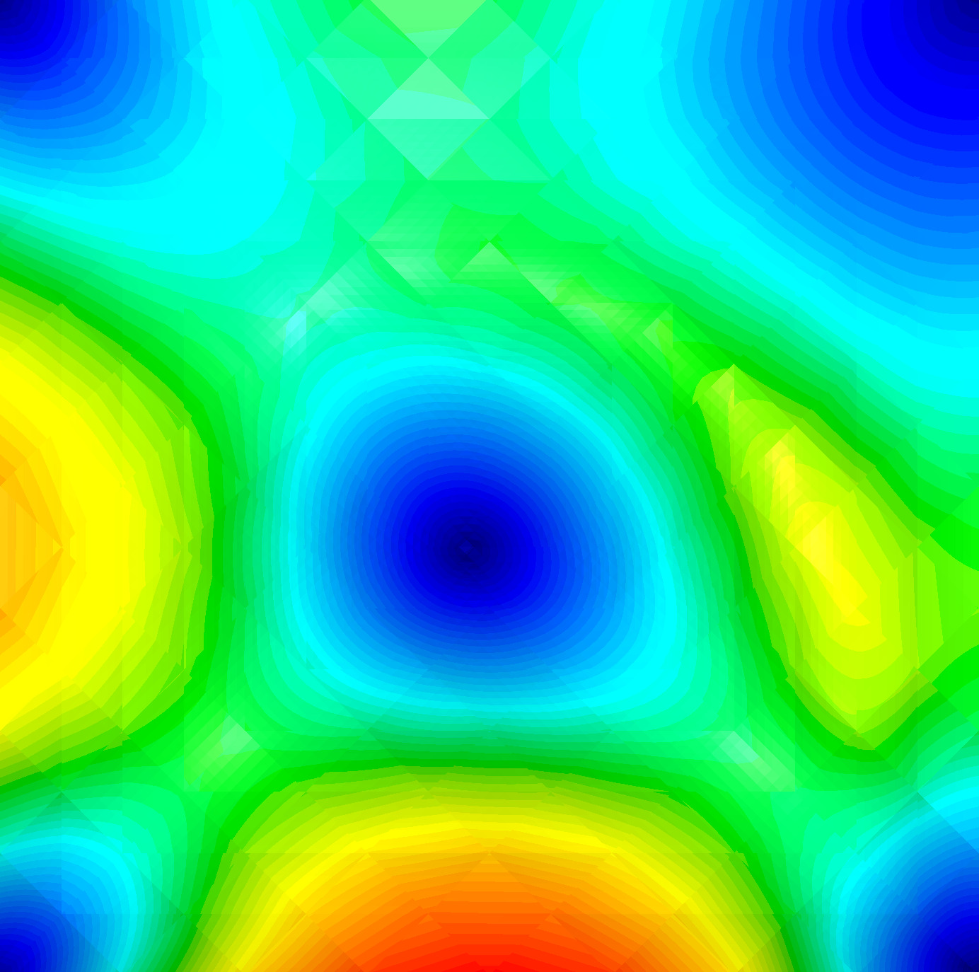
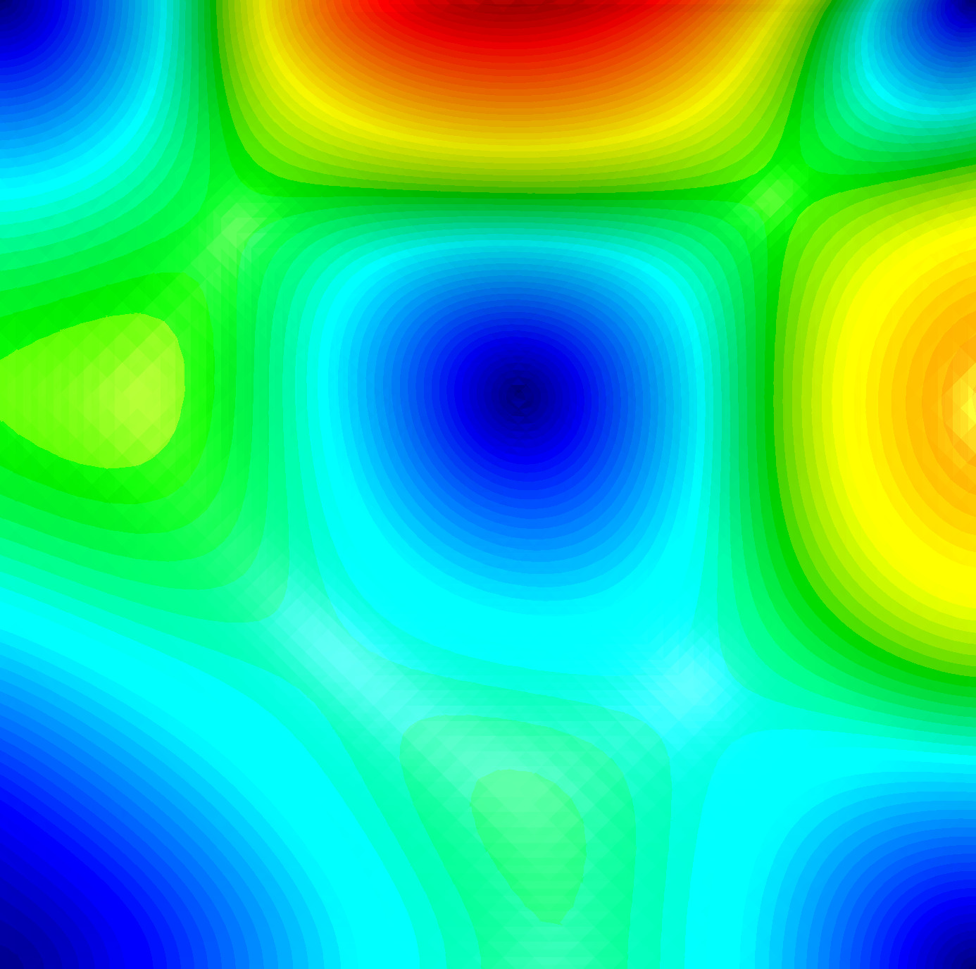
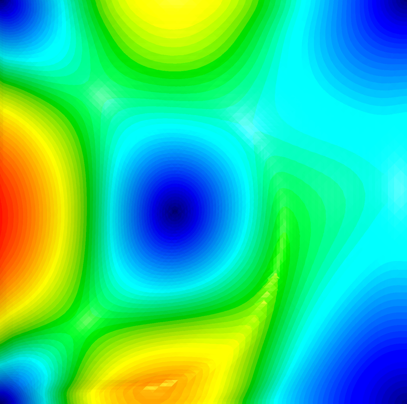
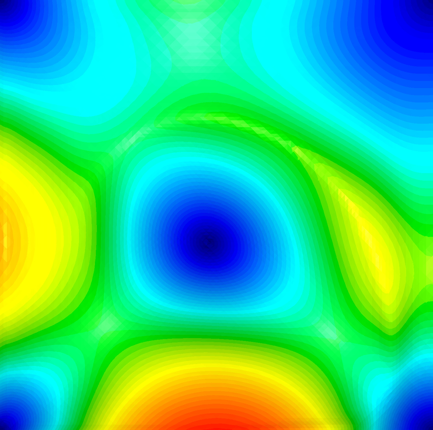
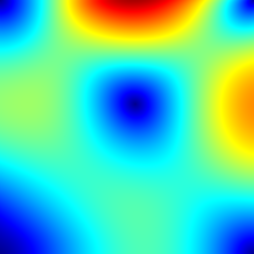
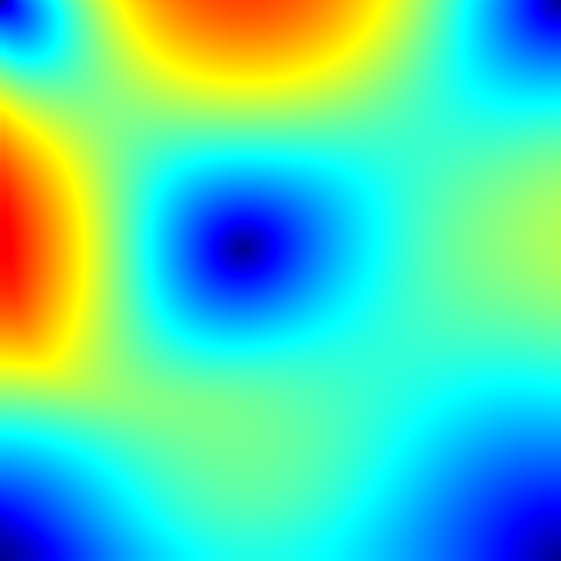
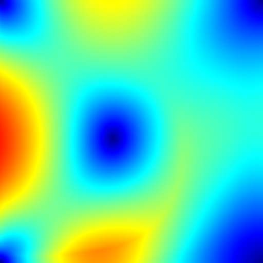
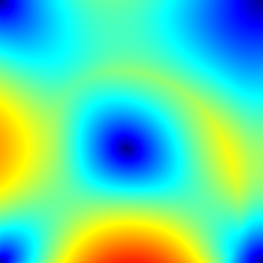
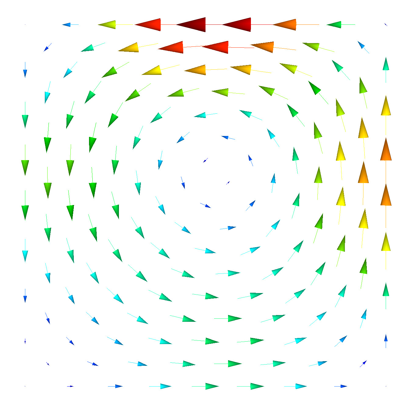
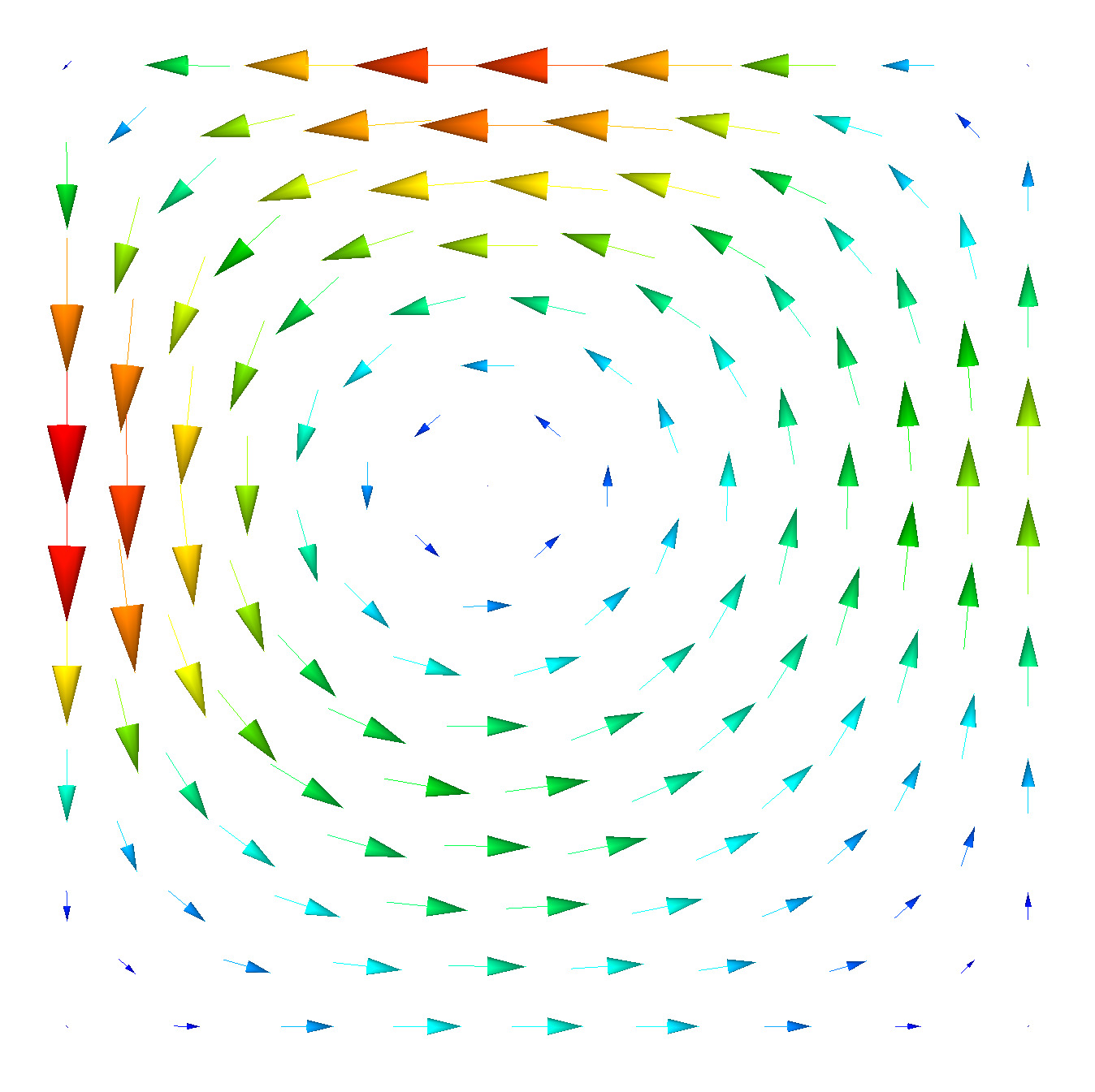
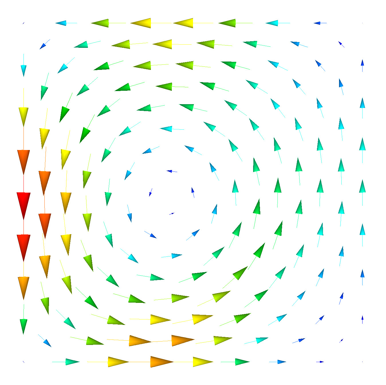
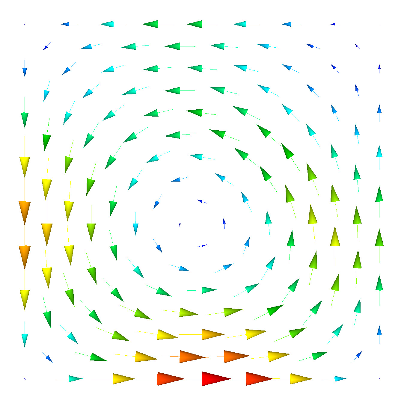
5.3 Experiment 3: A rotating hump problem

The Taylor-Green vortices provide exact solutions to the incompressible Navier-Stokes equations, but they are rather ”static” solutions. In this experiment, we consider a more dynamic solution. Let us consider the incompressible Navier-Stokes equations with $\Omega=[-\frac{1}{2},\frac{1}{2}]^{2}$, $T=1$, $\epsilon=0$, $f=0$, and vanishing normal boundary conditions. We consider the following initial condition

$$\boldsymbol{u}_{0}(\boldsymbol{x})=\begin{bmatrix}-\pi e^{x_{1}}\cos(\pi x_{1})\sin(\pi x_{2})\\ \pi e^{x_{1}}\sin(\pi x_{1})\cos(\pi x_{2})-e^{x_{1}}\cos(\pi x_{1})\cos(\pi x_{2})\end{bmatrix}.$$ (40)

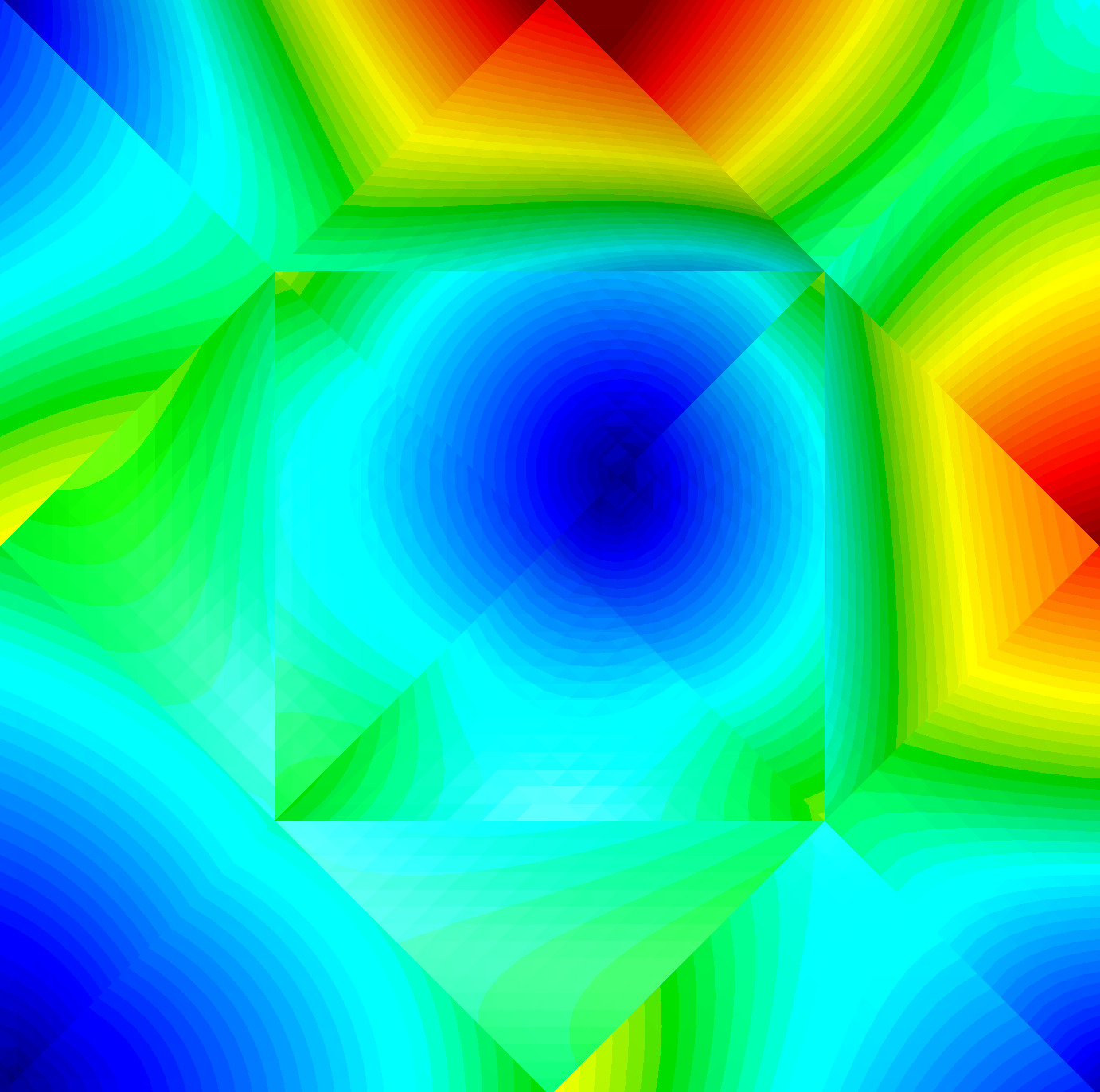
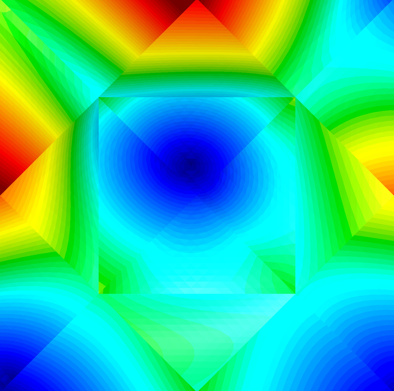
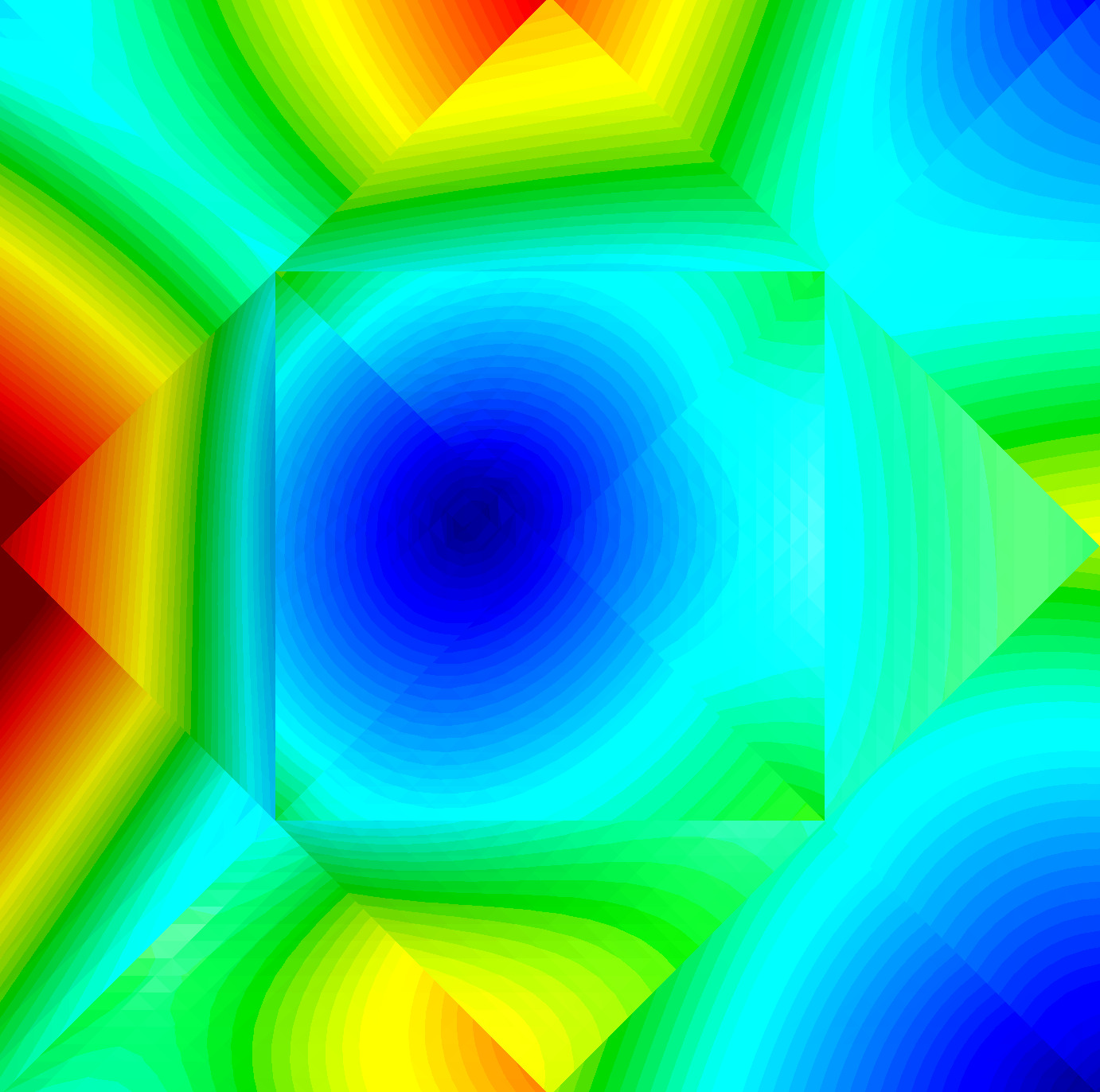
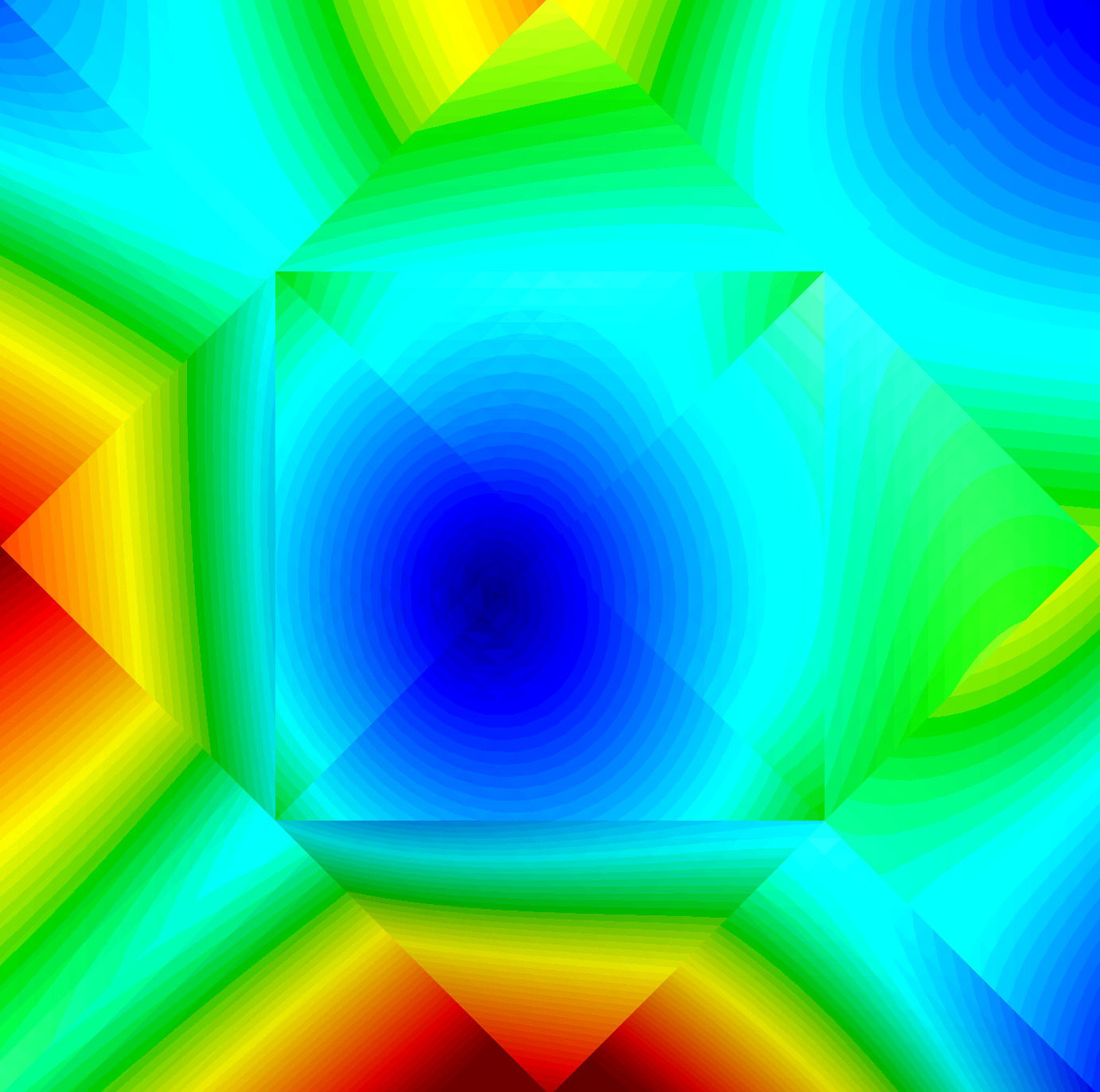
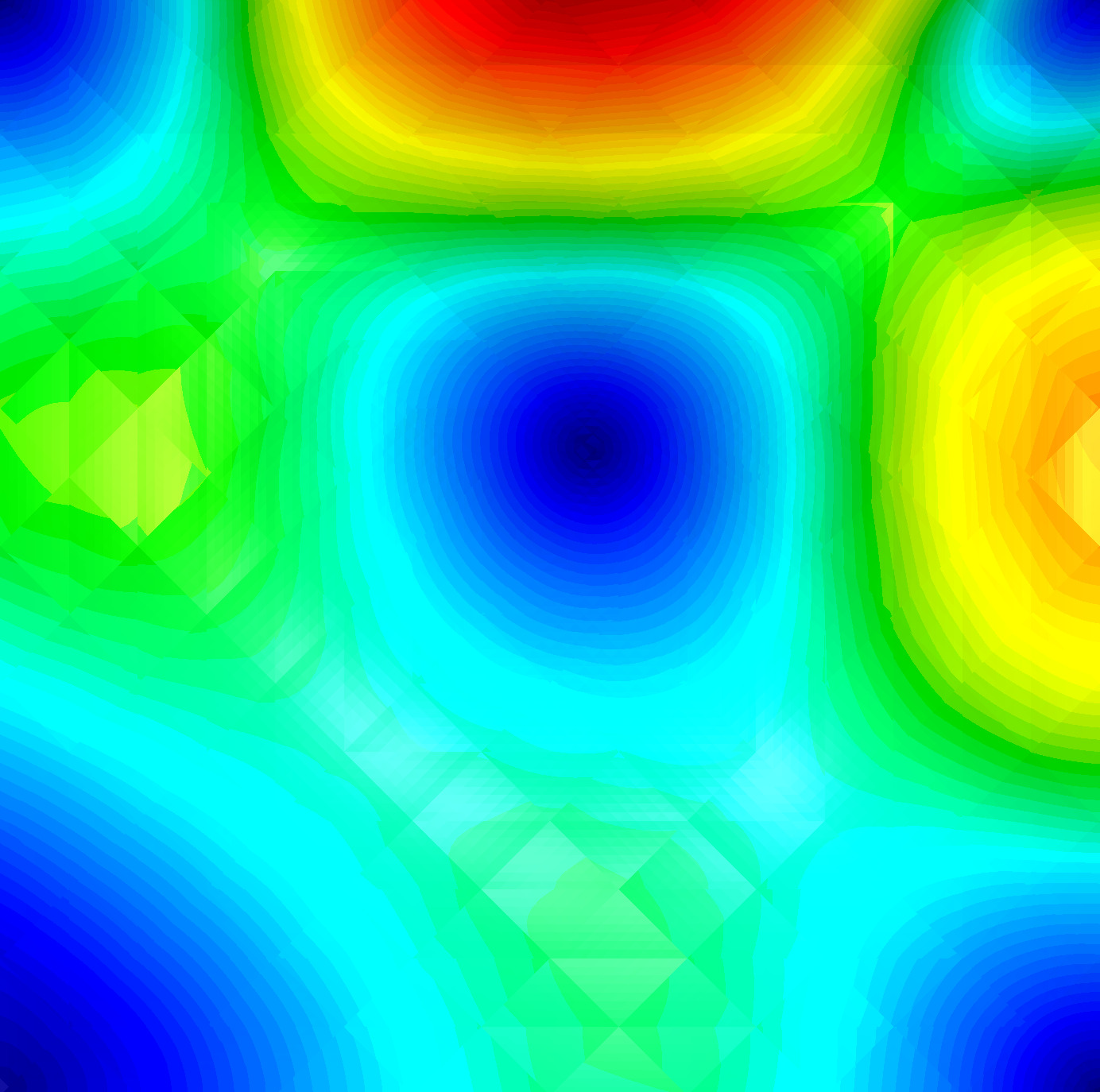
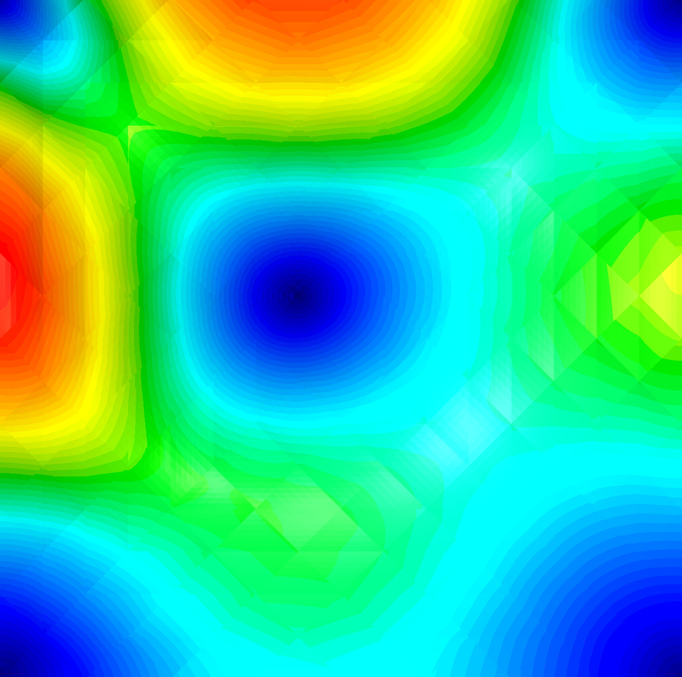
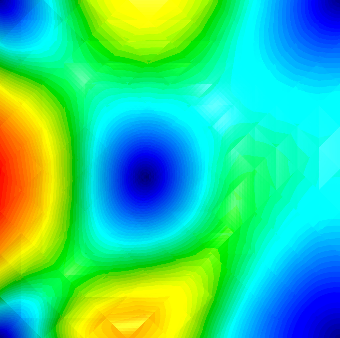
The exact solution to this problem is unknown, so we compare the solution computed by our scheme to the solution produced by the incompressible Euler solver Gerris [37]. The algorithm used in this solver is described in [36]. We computed the solution to this problem using the second-order, energy-tracking scheme presented in this work. Then, we plotted the magnitude of the computed velocity vector field for different mesh-sizes and time-steps at different time instances in Figures 14, 14, 14 and 14. Note that different visualisation tools were used to visualize the fields computed using the different solvers, but we observe that the solution computed by the semi-Lagrangian scheme comes visually closer to the solution computed by Gerris as we decrease the mesh width and time step. This is confirmed by Figure 9, where we display the L2 error between the solution computed using the semi-Lagrangian scheme and the solution computed using Gerris. In Figure 15, we display the vector field as computed using the second-order, conservative semi-Lagrangian scheme.

Also, in Figure 16 we display the values of the L2 norm over time of the solutions produced using our first- and second-, energy-tracking and non-energy-tracking schemes. Note that the energy-tracking schemes preserve the L2 norm as expected. The first-order, non-conservative scheme seems unstable at first, but in reality the ordinate axis spans a very small range and it turns out that the L2 norm converges to a bounded value for longer run-times.

Figure 9: Convergence results for Experiment 3 using the second-order, conservative scheme on simplicial meshes with mesh width $h$, timestep $\tau=0.06580h$, and final time $T=1$. The reference solution is a solution computed by Gerris [36]

(a) $t=0.25$

(b) $t=0.5$

(c) $t=0.75$

(d) $t=1$

Figure 10: Experiment 3: mesh width $h=0.379918$ and time-step $\tau=0.025$.

(e) $t=0.25$

(f) $t=0.5$

(g) $t=0.75$

(h) $t=1$

Figure 11: Experiment 3: mesh width $h=0.0949795$ and time-step $\tau=0.00625$.

(a) $t=0.25$

(b) $t=0.5$

(c) $t=0.75$

(d) $t=1$

Figure 12: Experiment 3: mesh width $h=0.023744875$ and time-step $\tau=0.0015625$.

(a) $t=0.25$

(b) $t=0.5$

(c) $t=0.75$

(d) $t=1$

Figure 13: Reference solution Experiment 3 computed using [37].

Figure 14: Colorbar associated with Figures 14, 14, 14 and 14

(a) $t=0.25$

(b) $t=0.5$

(c) $t=0.75$

(d) $t=1$

Figure 15: Velocity field for Experiment 3 computed using the second-order, conservative semi-Lagrangian scheme on a simplicial mesh with mesh width $h=0.189959$ and time-step $\tau=0.0125$. The colors indicate the magnitude of the vector.

Figure 16: The L2 norm of the computed solutions for Experiment 3 using different variants of the semi-Lagrangian scheme on a simplicial mesh with mesh width $h=0.04748975$ and time-step $\tau=0.003125$. In the legend, ’cons’ is short for ’conservative’ and refers to energy-tracking schemes. We use $\epsilon=0$ and $f=0$. In this figure, the time-step is too small to indicate samples by stars as done in similar figures.

5.4 Experiment 4: A transient solution in 3D

To verify the scheme for transient solutions in 3D, we consider the incompressible Navier-Stokes equations with $\Omega=[-\frac{1}{2},\frac{1}{2}]^{3}$, $T=1$, $\epsilon=0$, and both the normal boundary conditions and $f$ are chosen such that

$$\boldsymbol{u}(t,\boldsymbol{x})=\begin{bmatrix}-x_{2}\pi\cos(\frac{t}{4}+\pi x_{2}x_{3})\cos(\pi x_{2})\\ -x_{3}\pi\cos(\frac{t}{4}+\pi x_{1}x_{3})\cos(\pi x_{3})\\ -x_{1}\pi\cos(\frac{t}{4}+\pi x_{1}x_{2})\cos(\pi x_{1})\end{bmatrix}$$ (41)

is a solution. We ran a simulation for different mesh-sizes with time-steps determined by a suitable CFL condition. We summarize the results in Figure 17. We observe second-order convergence for the second-order scheme. The first-order scheme seems to achieve an order of convergence that is between first- and second-order, but this may be pre-asymptotic behaviour.

Figure 17: Convergence results for Experiment 4 using the first- and second-order schemes without energy-tracking on simplicial meshes with mesh width $h$, timestep $\tau=\frac{1}{\sqrt{2}}h$.

5.5 Experiment 5: Lid-driven cavity with slippery walls

In this section, we simulate a situation that resembles a lid-driven cavity problem. Consider the incompressible Navier-Stokes with $\Omega=[-\frac{1}{2},\frac{1}{2}]^{2}$, $T=7.93$, $\epsilon=0$, vanishing normal boundary conditions and the initial velocity field is set equal to zero. Then, to simulate a moving lid at the top, we apply the force-field $\boldsymbol{f}(t,\boldsymbol{x})=[v(\boldsymbol{x}),0]^{T}$ with

$$v(\boldsymbol{x})=\begin{cases}\text{exp}\left(1-\frac{1}{1-100(0.5-x_{2})^{2}}\right),&\text{if }1-100(0.5-x_{2})^{2}>0,\\ 0,&\text{else}.\end{cases}$$ (42)

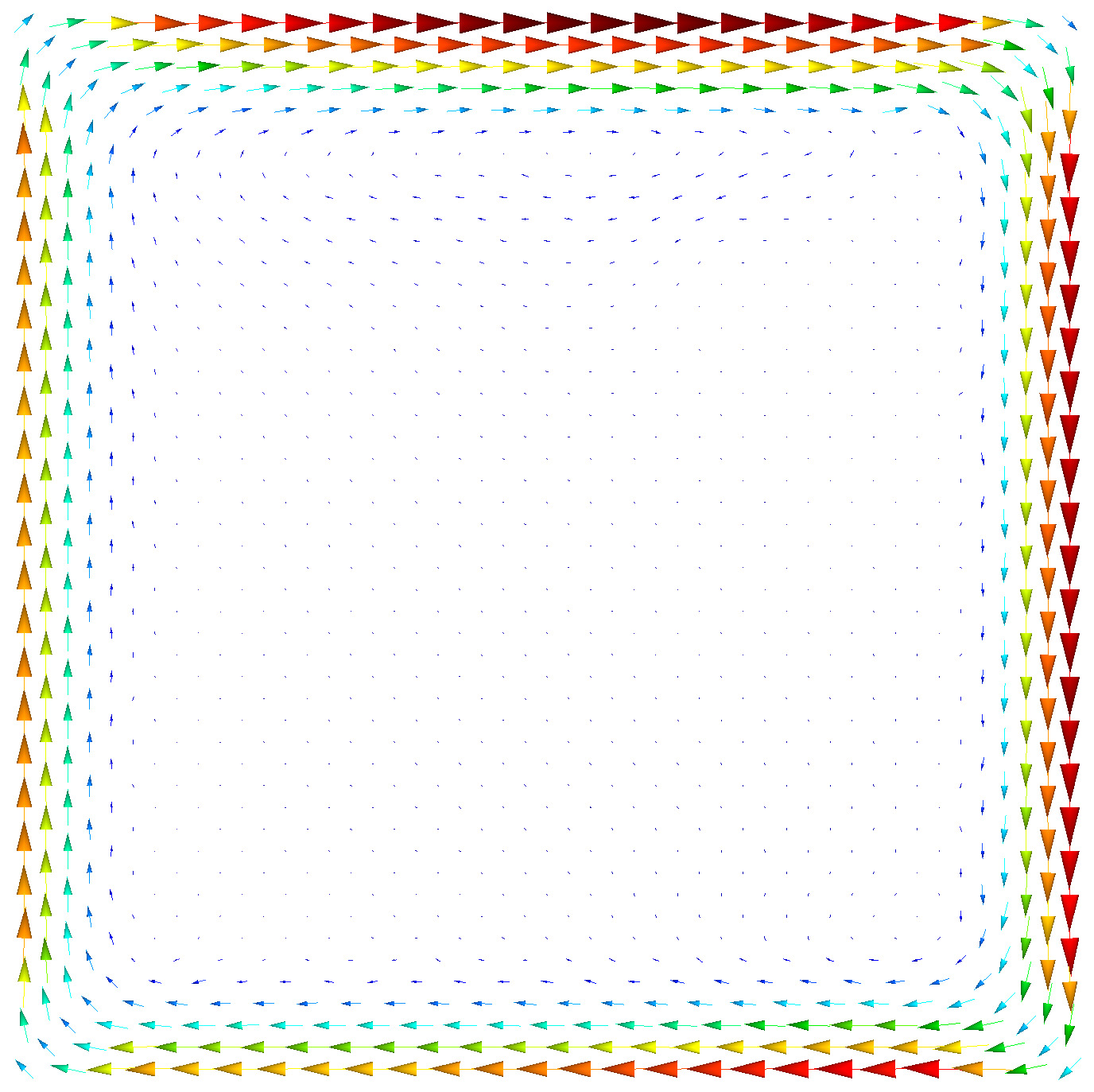
This force field gives a strong force in the $x_{1}$-direction close to the top lid, but quickly tapers off to zero as we go further from the top lid. In Figure 18, we display the computed velocity field. Note that, because we apply slip boundary conditions, we do not expect to observe vortices. The numerical solution reproduces this expectation.

Figure 18: Velocity field at $T=7.93s$ of Experiment 5 computed using the second-order, non-conservative semi-Lagrangian scheme on a simplicial mesh with mesh width $h=0.189959$ and $\tau=0.01$.

5.6 Experiment 6: A more complicated domain

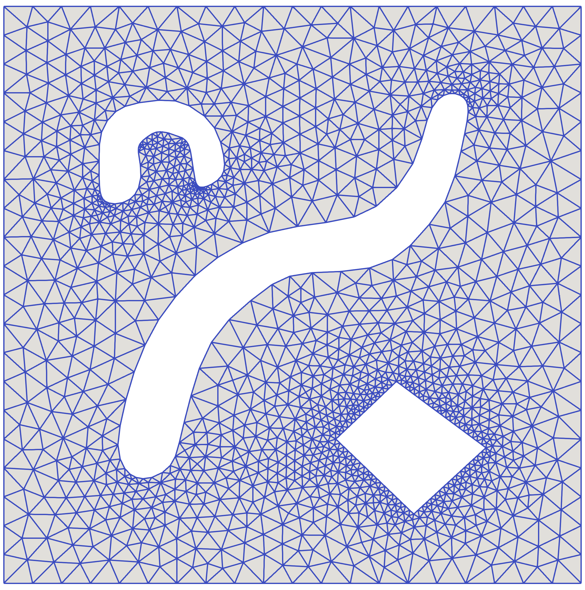
The numerical experiments given above, show the convergence and conservative properties of the introduced schemes. However, these experiments are all performed on very simple, rectangular domains. In this experiment, we consider a more complicated domain and mesh (generated using [22]) as shown in Figure 19.

We consider the case of the incompressible Navier-Stokes equations on the domain as given in Figure 19, $T=100$, $\epsilon=0$, $f=0$ and vanishing normal boundary conditions. We need to construct an initial condition that is divergence-free with vanishing normal boundary conditions. Following an approach close to a Chorin projection, we start with

$$\boldsymbol{w}(x,y)=\begin{bmatrix}\sin\big{(}2\cos(\sqrt{x^{2}+y^{2}})-\textrm{atan2}(y,x)\big{)}\\ \sin\big{(}\cos(\sqrt{x^{2}+y^{2}})-2\textrm{ atan2}(y,x)\big{)}\end{bmatrix}.$$ (43)

We use this definition to define a scalar function, $\phi$, as

$$\Delta\phi =\nabla\cdot\boldsymbol{w} \text{in }\Omega,$$ (44)

$$\nabla\phi\cdot\hat{n} =\boldsymbol{w}\cdot\hat{n} \text{on }\partial\Omega.$$ (45)

We can define our initial condition, $\boldsymbol{u}_{0}$, as

$$\boldsymbol{u}_{0}=\boldsymbol{w}-\nabla\phi$$ (46)

Note that $\boldsymbol{u}_{0}$ is divergence-free and has vanishing normal boundary conditions. The above system of equations can be solved using an appropriate finite-element implementation.

Note that in this experiment, the field outside the domain is unknown. This is well-defined on a continuous level, since vanishing boundary conditions imply that no particle will flow in from outside the domain. However, on the discrete level we cannot guarantee that the same will happen. It could happen that a part of a transported edge (as discussed in section 3.2) ends up outside the domain. In this case, we will assume that the average of the vector field along the part of the edge that lies outside the domain, will have the same value as the average of the corresponding edge in its original location (before transport) at the previous timestep.

The first ten seconds were simulated and a video of the results can be found at https://youtu.be/Eica8XHLtxY. For the different schemes, we also tracked the energy in Figure 20.

Figure 19: Domain and mesh associated with Experiment 6.

Figure 20: The L2 norm of the computed solutions for Experiment 6 using different variants of the semi-Lagrangian scheme on a simplicial mesh as given in Figure 19 and time-step $\tau=0.01$. In the legend, ’cons’ is short for ’conservative’ and refers to energy-tracking schemes. In this figure, the time-step is too small to indicate samples by stars as done in similar figures.

6 Conclusion

We have developed a mesh-based semi-Lagrangian discretization of the time-dependent incompressible Navier-Stokes equations with free boundary conditions recast as a non-linear transport problem for a momentum 1-form. A linearly implicit fully discrete version of the scheme enjoys excellent stability properties in the vanishing-viscosity limit and is applicable to inviscid incompressible Euler flows. However, in this case conservation of energy has to be enforced separately. Making the reasonable choice of a time-step size proportional to the mesh width, the algorithm involves only local computations. Yet, these are significantly more expensive compared to those required for purely Eulerian finite-element and finite-volume methods. At this point the verdict on the competitiveness of our semi-Lagrangian scheme is still open.

Statements and Declarations

The authors have no financial or other conflicts of interest to declare.

Appendix A Two formulations of the momentum equation

Consider the momentum equation in (1)

$$\partial_{t}\boldsymbol{u}+\boldsymbol{u}\cdot\nabla\boldsymbol{u}-\epsilon\Delta\boldsymbol{u}+\nabla p=\boldsymbol{0}.$$

Note that we have by standard vector calculus identities

$$\Delta\boldsymbol{u}=\nabla(\nabla\cdot\boldsymbol{u})-\nabla\times\nabla\times\boldsymbol{u},$$

where we can use $\nabla\cdot\boldsymbol{u}=0$ to obtain

$$\Delta\boldsymbol{u}=-\nabla\times\nabla\times\boldsymbol{u}.$$

This allows us to rewrite the momentum equation as

$$\partial_{t}\boldsymbol{u}+\boldsymbol{u}\cdot\nabla\boldsymbol{u}+\epsilon\nabla\times\nabla\times\boldsymbol{u}+\nabla p=\boldsymbol{0}.$$

Using the gradient of the dot-product, we find

$$\nabla(\boldsymbol{u}\cdot\boldsymbol{u})=2\boldsymbol{u}\cdot\nabla\boldsymbol{u}+2\boldsymbol{u}\times(\nabla\times\boldsymbol{u}).$$

This identity allows us to rewrite the momentum equation to

$$\partial_{t}\boldsymbol{u}+\nabla(\boldsymbol{u}\cdot\boldsymbol{u})-\boldsymbol{u}\times(\nabla\times\boldsymbol{u})+\epsilon\nabla\times\nabla\times\boldsymbol{u}+\nabla\left(-\frac{1}{2}\boldsymbol{u}\cdot\boldsymbol{u}+p\right)=\boldsymbol{0}.$$

From [27, 25], we obtain the identity

$$\left(\text{L}_{\boldsymbol{u}}\omega\right)^{\musSharp{}}=\nabla(\boldsymbol{u}\cdot\boldsymbol{u})-\boldsymbol{u}\times(\nabla\times\boldsymbol{u})$$

where $\omega$ is the differential 1-form such that $\boldsymbol{u}=\omega^{\musSharp{}}$. Since the material derivative for this 1-form is

$$D_{\boldsymbol{u}}\omega\coloneqq\partial_{t}\omega+\text{L}_{\boldsymbol{u}}\omega,$$

we find that the momentum equation can be written as

$$D_{\boldsymbol{u}}\omega+\epsilon\delta\text{d}\omega+\text{d}\tilde{p}=0,$$

where $\tilde{p}=-\frac{1}{2}\boldsymbol{u}\cdot\boldsymbol{u}+p$.

References

• \bibcommenthead
• Anderson et al [2021] Anderson R, Andrej J, Barker A, et al (2021) MFEM: A modular finite element methods library. Computers and Mathematics with Applications 81. 10.1016/j.camwa.2020.06.009
• Arnold [2018] Arnold DN (2018) Finite Element Exterior Calculus. 10.1137/1.9781611975543
• Arnold et al [2006] Arnold DN, Falk RS, Winther R (2006) Finite element exterior calculus, homological techniques, and applications. Acta Numerica 15:1–155. 10.1017/S0962492906210018
• Arnold [1966] Arnold V (1966) Sur la géométrie différentielle des groupes de Lie de dimension infinie et ses applications à l’hydrodynamique des fluides parfaits. Annales de L’Institut Fourier 16:319–361. URL http://www.numdam.org/articles/10.5802/aif.233/
• Bause and Knabner [2002] Bause M, Knabner P (2002) Uniform error analysis for Lagrange-Galerkin approximations of convection-dominated problems. SIAM Journal on Numerical Analysis 39(6):1954–1984. 10.1137/S0036142900367478
• Bercovier and Pironneau [1982] Bercovier M, Pironneau O (1982) Characteristics and the finite element method. In: Finite Element Flow Analysis, pp 67–73, URL https://ui.adsabs.harvard.edu/abs/1982fefa.proc...67B
• Bercovier et al [1983] Bercovier M, Pironneau O, Sastri V (1983) Finite elements and characteristics for some parabolic-hyperbolic problems. Applied Mathematical Modelling 7(2):89–96. 10.1016/0307-904X(83)90118-X
• Bermejo and Saavedra [2012] Bermejo R, Saavedra L (2012) Modified Lagrange-Galerkin methods of first and second order in time for convection-diffusion problems. Numerische Mathematik 120(4). 10.1007/s00211-011-0418-8
• Bermejo and Saavedra [2015] Bermejo R, Saavedra L (2015) Modified Lagrange–Galerkin Methods to Integrate Time Dependent Incompressible Navier–Stokes Equations. SIAM Journal on Scientific Computing 37(6):B779–B803. 10.1137/140973967
• Bermejo and Saavedra [2016] Bermejo R, Saavedra L (2016) Lagrange–Galerkin methods for the incompressible Navier-Stokes equations: a review. Communications in Applied and Industrial Mathematics 7(3):26–55. 10.1515/caim-2016-0021
• Bermejo et al [2012] Bermejo R, Galán Del Sastre P, Saavedra L (2012) A Second Order in Time Modified Lagrange–Galerkin Finite Element Method for the Incompressible Navier–Stokes Equations. SIAM Journal on Numerical Analysis 50(6):3084–3109. 10.1137/11085548X
• Bonaventura et al [2018] Bonaventura L, Ferretti R, Rocchi L (2018) A fully semi-Lagrangian discretization for the 2D incompressible Navier–Stokes equations in the vorticity-streamfunction formulation. Applied Mathematics and Computation 323:132–144. 10.1016/j.amc.2017.11.030
• Boukir et al [1994] Boukir K, Maday Y, Métivet B (1994) A high order characteristics method for the incompressible Navier–Stokes equations. Computer Methods in Applied Mechanics and Engineering 116(1-4):211–218. 10.1016/S0045-7825(94)80025-1
• Buscaglia and Dari [1992] Buscaglia GC, Dari EA (1992) Implementation of the Lagrange-Galerkin method for the incompressible Navier-Stokes equations. International Journal for Numerical Methods in Fluids 15(1):23–36. 10.1002/fld.1650150103
• Celledoni et al [2003] Celledoni E, Marthinsen A, Owren B (2003) Commutator-free Lie group methods. Future Generation Computer Systems 19(3):341–352. 10.1016/S0167-739X(02)00161-9
• Celledoni et al [2016] Celledoni E, Kometa BK, Verdier O (2016) High Order Semi-Lagrangian Methods for the Incompressible Navier–Stokes Equations. Journal of Scientific Computing 66(1):91–115. 10.1007/s10915-015-0015-6
• Chorin and Marsden [1993] Chorin AJ, Marsden JE (1993) A mathematical introduction to fluid mechanics. 10.1007/978-1-4612-0883-9
• De Rosa [2020] De Rosa L (2020) On the Helicity conservation for the incompressible Euler equations. Proceedings of the American Mathematical Society 148(7):2969–2979. 10.1090/proc/14952
• Douglas and Russell [1982] Douglas JJr., Russell TF (1982) Numerical methods for convection-dominated diffusion problems based on combining the method of characteristics with finite element or finite difference procedures. SIAM J Numer Anal 19(5):871–885. 10.1137/0719063
• El-Amrani and Seaid [2011] El-Amrani M, Seaid M (2011) An L2-projection for the Galerkin-characteristic solution of incompressible flows. SIAM Journal on Scientific Computing 33(6):3110–3131. 10.1137/100805790
• Ewing et al [1984] Ewing RE, Russell TF, Wheeler MF (1984) Convergence analysis of an approximation of miscible displacement in porous media by mixed finite elements and a modified method of characteristics. Computer Methods in Applied Mechanics and Engineering 47(1-2):73–92. 10.1016/0045-7825(84)90048-3
• Geuzaine and Remacle [2009] Geuzaine C, Remacle JF (2009) Gmsh: A 3-D finite element mesh generator with built-in pre- and post-processing facilities. International Journal for Numerical Methods in Engineering 79(11):1309–1331. 10.1002/nme.2579
• Hasbani et al [1983] Hasbani Y, Livne E, Bercovier M (1983) Finite elements and characteristics applied to advection-diffusion equations. Computers & Fluids 11(2):71–83. 10.1016/0045-7930(83)90002-6
• Heumann and Hiptmair [2011] Heumann H, Hiptmair R (2011) Eulerian and semi-lagrangian methods for convection-diffusion for differential forms. PhD thesis, 10.3929/ethz-a-006506738
• Heumann and Hiptmair [2013] Heumann H, Hiptmair R (2013) Convergence of Lowest Order Semi-Lagrangian Schemes. Foundations of Computational Mathematics 13(2):187–220. 10.1007/s10208-012-9139-3
• Heumann et al [2012] Heumann H, Hiptmair R, Li K, et al (2012) Fully discrete semi-Lagrangian methods for advection of differential forms. BIT Numerical Mathematics 52(4):981–1007. 10.1007/s10543-012-0382-4
• Hiptmair [2002] Hiptmair R (2002) Finite elements in computational electromagnetism. Acta Numerica 11:237–339. 10.1017/S0962492902000041
• Isett [2018] Isett P (2018) A proof of Onsager’s conjecture. Annals of Mathematics 188(3):871–963. 10.4007/annals.2018.188.3.4
• Karniadakis and Sherwin [2005] Karniadakis G, Sherwin S (2005) Spectral/hp Element Methods for Computational Fluid Dynamics. 10.1093/acprof:oso/9780198528692.001.0001
• Minev and Ross Ethier [1999] Minev PD, Ross Ethier C (1999) A characteristic/finite element algorithm for the 3-D Navier–Stokes equations using unstructured grids. Computer Methods in Applied Mechanics and Engineering 178(1-2):39–50. 10.1016/S0045-7825(99)00003-1
• Mitrea and Monniaux [2009] Mitrea M, Monniaux S (2009) The nonlinear Hodge-Navier-Stokes equations in Lipschitz domains. Differential and Integral Equations 22(3/4):339–356. 10.57262/die/1356019778
• Morton et al [1988] Morton K, Priestley A, Suli E (1988) Stability of the Lagrange-Galerkin method with non-exact Integration. Mathematical Modelling and Numerical Analysis 22(4):625–653. URL http://www.numdam.org/item/M2AN_1988__22_4_625_0/
• Natale and Cotter [2018] Natale A, Cotter CJ (2018) A variational H(div) finite-element discretization approach for perfect incompressible fluids. IMA Journal of Numerical Analysis 38(3):1388–1419. 10.1093/imanum/drx033
• Patera [1984] Patera AT (1984) A spectral element method for fluid dynamics: Laminar flow in a channel expansion. Journal of Computational Physics 54(3):468–488. 10.1016/0021-9991(84)90128-1
• Pironneau [1982] Pironneau O (1982) On the transport-diffusion algorithm and its applications to the Navier-Stokes equations. Numerische Mathematik 38(3):309–332. 10.1007/BF01396435
• Popinet [2003] Popinet S (2003) Gerris: a tree-based adaptive solver for the incompressible Euler equations in complex geometries. Journal of Computational Physics 190(2):572–600. 10.1016/S0021-9991(03)00298-5
• Popinet [2007] Popinet S (2007) The Gerris Flow Solver. URL https://gfs.sourceforge.net/wiki/index.php/Main_Page
• Rapetti and Bossavit [2009] Rapetti F, Bossavit A (2009) Whitney Forms of Higher Degree. SIAM Journal on Numerical Analysis 47(3):2369–2386. 10.1137/070705489
• Russell [1985] Russell TF (1985) Time stepping along characteristics with incomplete iteration for a Galerkin approximation of miscible displacement in porous media. SIAM J Numer Anal 22(5):970–1013. 10.1137/0722059
• Süli [1988] Süli E (1988) Convergence and nonlinear stability of the Lagrange-Galerkin method for the Navier-Stokes equations. Numerische Mathematik 53(4):459–483. 10.1007/BF01396329
• Süli and Mayers [2003] Süli E, Mayers DF (2003) An Introduction to Numerical Analysis. 10.1017/CBO9780511801181
• Taylor and Green [1937] Taylor GI, Green AE (1937) Mechanism of the production of small eddies from large ones. Proceedings of the Royal Society of London Series A-Mathematical and Physical Sciences 158(895):499–521. 10.1098/rspa.1937.0036
• Temam and Ziane [1996] Temam R, Ziane M (1996) Navier-Stokes equations in three-dimensional thin domains with various boundary conditions. Advances in Differential Equations 1(4):499–546. ade/1366896027
• Vuik et al [2015] Vuik C, Vermolen FJ, Gijzen MB, et al (2015) Numerical methods for ordinary differential equations. s10915-004-4647-1
• Wang and Wang [2010] Wang H, Wang K (2010) Uniform Estimates of an Eulerian–Lagrangian Method for Time-Dependent Convection-Diffusion Equations in Multiple Space Dimensions. SIAM Journal on Numerical Analysis 48(4):1444–1473. 10.1137/070682952
• Xiu and Karniadakis [2001] Xiu D, Karniadakis GE (2001) A Semi-Lagrangian High-Order Method for Navier–Stokes Equations. Journal of Computational Physics 172(2):658–684. 10.1006/jcph.2001.6847
• Xiu et al [2005] Xiu D, Sherwin SJ, Dong S, et al (2005) Strong and auxiliary forms of the semi-Lagrangian method for incompressible flows. Journal of Scientific Computing 25(1):323–346. 10.1007/s10915-004-4647-1