Full non–LTE spectral line formation II. Two–distribution radiation transfer with coherent scattering in the atom’s frame

Abstract

In the present article, we discuss a numerical method of solution for the so-called “full non-LTE” radiation transfer problem, basic formalism of which was revisited by Paletou & Peymirat (2021; see also Oxenius 1986). More specifically, usual numerical iterative methods for non-LTE radiation transfer are coupled with the above-mentioned formalism. New numerical additions are explained in detail. We benchmark the whole process with the standard non-LTE transfer problem for a two-level atom with Hummer’s (1962, 1969) $R_{\rm I-A}$ partial frequency redistribution function. We finally display new quantities such as the spatial distribution of the velocity distribution function of excited atoms, that can only be accessed to by adopting this more general frame for non-LTE radiation transfer.

I Introduction

Oxenius (1986) formulated the so-called “full non-LTE” radiation transfer problem, wherein the distribution of photons as well as the massive particles in a stellar atmosphere may in general both deviate from their equilibrium distributions. Paletou & Peymirat (2021, hereafter PP21) revisited this formalism and rediscussed some basic elements using standard notations prevalent in this field of research. In PP21, we however, limited ourselves to the more detailed statistical equilibrium equations for the simplest case of a “two-distribution” model.

The present study is devoted to the coupling of that formalism with usual numerical methods used for radiation transfer. The set and sequence of the new quantities required for our computations are outlined in §2 hereafter, in the continuation and sometimes the generalization of relationships previously discussed in PP21.

The validation of these new elements, dealing directly with the coupling of the frequency dependence of the radiation and the velocities of the atoms scattering light, is first made for the case of coherent scattering in the atom’s frame. We can indeed show – see §3 – that the latter assumption for our two-distribution problem makes it equivalent to a two-level atom problem with the standard angle-averaged partial frequency redistribution (PRD) function $R_{\rm I-A}$ for isotropic scattering introduced by Hummer (1962).

Useful details about the very numerical implementation of our new computations are exposed in §4 and a simple iterative scheme is described in §5. We fully rely on a nowadays quite usual short-characteristics formal solver, mostly used for iterative methods such as accelerated $\Lambda$-iteration (hereafter ALI), whose material was developed and made available by us in Python (see e.g., Lambert et al. 2016 and references therein).

A first, indispensable validation is presented in §6, by reproducing results for standard PRD-$R_{\rm I-A}$ of Hummer (1969). It is however shown that, the two-distribution model provides additional physical quantities, which cannot be accessed to using the classical non-LTE framework, such as the spatial distribution of the velocity distribution function (hereafter VDF; see §6 and 8) of the excited atoms.

Sections 7 and 8 therefore present, respectively, a preliminary exploration of the effects of velocity-changing elastic collisions, and new computations for a strongly illuminated finite slab case.

We finally discuss the various perspectives of this study.

II Coupling to radiation transfer

The implementation of our kinetic approach together with radiation transfer requires, in a first place, two major modifications of existing numerical radiation transfer tools.

In the following, and after Paletou & Peymirat (2021), we shall adopt both the reduced frequency $x$, and the normalized atomic velocity $u$. The reduced frequency is usually defined in radiation transfer as $x=(\nu-\nu_{0})/\Delta\nu_{D}$ that is the frequency shift from the line center normalized to the Doppler width $\Delta\nu_{D}=(\nu_{0}/c)v_{th.}$, where $c$ is the speed of light; while $u$ is the modulus of the atomic velocity normalized to the “most probable velocity” $v_{th.}=\sqrt{2kT/M}$, with $k$ being the Boltzmann constant, $T$ the temperature, and $M$ the mass of the atom.

The first requirement is the computation of the scattering integral $J_{12}$ defined as:

$$J_{12}(\vec{u},\tau)=\oint{{{d\Omega}\over{4\pi}}}\int{\delta(x-\vec{u}\cdot\vec{\Omega})I(x,\vec{\Omega},\tau)dx}\,,$$ (1)

in the case of coherent scattering in the atomic frame, where $\delta$ is the Dirac distribution for the a priori known absorption profile and $I(x,\vec{\Omega},\tau)$ the usual specific intensity. The latter is computed at every frequency $x$, photon propagation direction $\vec{\Omega}$, and optical depth $\tau$ using a “classic” short characteristic based formal solver (see e.g. Lambert et al. 2016, and associated resources). Once this quantity is available, our modified formal solver calls a specific function which performs the angular integration over the Dirac distribution $\delta(x-\vec{u}\cdot\vec{\Omega})$, adapted from Sampoorna et al. (2011; see also §4).

In a second step, one computes $\bar{J}_{12}(\vec{u},\tau)={J}_{12}(\vec{u},\tau)/{\mathcal{B}}_{W}$ with ${\mathcal{B}}_{W}$ denoting the Planck function in the Wien limit, and:

$${\cal{J}}_{12}(\tau)=\int_{\vec{u}}{\bar{J}_{12}(\vec{u},\tau)f^{M}(\vec{u})d^{3}\vec{u}}\,,$$ (2)

with $f^{M}(\vec{u})={\rm e}^{-\vec{u}\cdot\vec{u}}/\pi^{3/2}$ for the Maxwellian velocity distribution. Here $d^{3}\vec{u}=u^{2}dud\Omega_{u}$ wherein $d\Omega_{u}=\sin\theta_{u}d\theta_{u}d\phi_{u}$, with $\theta_{u}$ and $\phi_{u}$ denoting the polar angles of the normalized atomic velocity vector $\vec{u}$ about the atmospheric normal.

Once we have computed these two quantities, we can evaluate the velocity distribution function of the first excited state of the atom using, as defined in PP21:

$$f_{2}(\vec{u},\tau)=\left[\frac{\zeta}{1+\zeta}+\left(\frac{1}{1+\zeta}\right)\frac{\varepsilon+(1-\varepsilon)\bar{J}_{12}(\vec{u},\tau)}{\varepsilon+(1-\varepsilon){\cal{J}}_{12}}\right]f^{M}(\vec{u})\,,$$ (3)

at every depth in the atmosphere. In this expression, $\varepsilon$ is the usual collisional destruction probability of standard non–LTE radiation transfer. However, another quantity $\zeta$ appears now, which characterizes the amount of velocity-changing elastic collisions defined in Eq. (27) of PP21 (note again that in PP21 the depth dependence of the different quantities such as $\bar{J}_{12}$, $f_{2}$ etc. were omitted, as radiative transfer was not considered in detail at this stage).

The next critical quantity is the computation of the emission profile, which is defined, at a given optical depth $\tau$ in our (1D) atmosphere as:

$$\psi(x,\tau)=\oint{{{d\Omega}\over{4\pi}}}\int_{\vec{u}}{\delta(x-\vec{u}\cdot\vec{\Omega})f_{2}(\vec{u},\tau)d^{3}\vec{u}}\,,$$ (4)

where $f_{2}$ is the VDF of the excited atoms scattering light, computed using Eq. (3). At this stage, we apply Eq. (A.1) of PP21 to first perform the integral over $d\Omega$ and then perform the integral over $d\Omega_{u}$ to give:

$$\psi(x,\tau)=\frac{2}{\sqrt{\pi}}\int_{\lvert x\rvert}^{\infty}{\left[\frac{\zeta}{1+\zeta}+\left(\frac{1}{1+\zeta}\right)\frac{\varepsilon+(1-\varepsilon)\tilde{J}_{12}(u,\tau)}{\varepsilon+(1-\varepsilon){\cal{J}}_{12}}\right]ue^{-u^{2}}du}\,,$$ (5)

where:

$$\tilde{J}_{12}(u,\tau)=\oint\bar{J}_{12}(\vec{u},\tau)d\Omega_{u}\,.$$ (6)

Clearly, the emission profile given in Eq. (5) above represents the generalization of the same analytical angular integration result in Eq. (42) of PP21 which however was written only for the $\zeta=0$ and $\varepsilon=0$ cases.

Once all the quantities defined by Eqs. (1)–(5) have been evaluated, one may then compute the source function. Hereafter we shall use the below expression, not given explicitly in PP21 though, for the source function:

$$S(x,\tau)=\left[\varepsilon+(1-\varepsilon){\cal{J}}_{12}(\tau)\right]\left[{{\psi(x,\tau)}\over{\varphi(x)}}\right]\,,$$ (7)

where $\varphi$ is the so-called Doppler absorption profile. It is quite straightforward to establish, and this is indeed the very expression of the source function that we used in the present study (note that this expression remains unchanged when $\zeta\neq 0$).

III Equivalence with Hummer’s $R_{\rm I-A}$ redistribution

It is easy to show that a “two-distribution” model assuming a Maxwellian distribution for $f_{1}$, characterizing the fundamental level, and coherent scattering in the atom’s frame is equivalent to a standard PRD model for a two–level atom problem considering Hummer’s angle-averaged (and isotropic scattering) $R_{\rm I-A}$ redistribution. It therefore provides a critical benchmark for our modified numerical tools.

A way to verify this equivalence is by using the developed expression of the emission profile given by the combination of Eqs. (3) and (4) together with Eq. (7). This should also be considered for $\zeta=0$ since this new parameter is not relevant to standard PRD using Hummer’s redistribution functions. Then, one may split in two the expression of the emission profile with a first part which goes like $\varepsilon f^{M}(\vec{u})$, and another one which implies $(1-\varepsilon)\bar{J}_{12}(\vec{u},\tau)f^{M}(\vec{u})$ – besides the common denominator which is independent from $\vec{u}$. The first part, after integrations, will lead to the Doppler absorption profile $\varphi$, since it is the convolution of the Dirac function characterizing coherent scattering in the atom’s frame with the Maxwellian VDF $f^{M}(\vec{u})$. But most interesting is however the second part involving $\bar{J}_{12}$. For this second part we go back to real frequencies $\xi$ (in the atomic frame) and $\nu$ (in the observer’s frame), from $x$ and the Doppler transform (see also notations adopted in PP21). Now the Dirac function appearing in Eq. (4) becomes $\delta(\xi-\nu_{0})$, while that in Eq. (1) when substituted in Eq. (4) becomes $\delta(\xi^{\prime}-\nu_{0})$. Thus, the second part of the emission profile contains the product of two Dirac distributions, namely $\delta(\xi-\nu_{0})\delta(\xi^{\prime}-\nu_{0})$. One can also rewrite this combination as: $\delta(\xi-\nu_{0})\delta(\xi^{\prime}-\xi)$ which is indeed the atomic redistribution function $r_{\rm I}$ (see e.g., Hubeny & Mihalas, 2014). This has also been discussed in §4 of Borsenberger et al. (1987).

After integration over velocities along the Maxwellian VDF, and after angular integration, we finally recover the more usual form of the standard PRD, frequency-dependent source function (normalized to the Planckian):

$$S(x,\tau)=\varepsilon+(1-\varepsilon)\oint{{{d\Omega^{\prime}}\over{4\pi}}}\int_{x^{\prime}}{\left[\frac{R_{\rm I-A}(x^{\prime},x)}{\varphi(x)}\right]I(x^{\prime},\Omega^{\prime},\tau)dx^{\prime}}\,.$$ (8)

And the solution of such a problem can easily be computed using the methods proposed by Paletou & Auer (1995).

IV Numerical implementation

Our numerical implementation of the new, full non-LTE problem relies on modifications brought to a nowadays classic short-characteristics (hereafter SC) based formal solver (see e.g. Lambert et al. 2016, and references therein). This, together with various iterative schemes which can be set on that basis constitutes a more efficient way, both fast and accurate, as well as easy to develop on, to address the problem than what was made previously by Borsenberger et al. (1986, 1987) and Atanackovi$\check{\rm c}$ et al. (1987).

The main numerical problem now, as compared to the standard non-LTE problem, is to properly evaluate expressions given by Eqs. (1) and (4). First is the angular integration for making $J_{12}$. It consists in using a quadrature in polar angle and azimuth $(\theta,\phi)$ both for the ray direction and for the atomic velocity. Then, one may write: $\vec{u}\cdot\vec{\Omega}=\gamma u$ where:

$$\gamma=\cos(\theta_{r})\cos(\theta_{u})+\sin(\theta_{r})\sin(\theta_{u})\cos(\phi_{r}-\phi_{u})\,.$$ (9)

Here indices $r$ and $u$ are respectively associated with the ray and the atomic velocity directions.

Once $\gamma$ has been computed for every couple of polar angle and azimuth, the specific intensity is interpolated in $x$ in order to estimate the $I(x=\gamma u)$ quantity that will contribute to the integral leading to $J_{12}(\vec{u},\tau)$, after a first integration in frequency along the atomic absorption profile. A mere linear interpolation was used together with our identical $x$ and $u$ grids, hereafter spanning 6 Doppler width in $x$, with $\Delta u=\Delta x=0.1$. To achieve this very task, we use a dedicated function which is called in from the usual SC formal solver, once the specific intensity is available at all frequencies, at a given depth and direction.

Practically, we used a 10-point regularly spaced quadrature for $\phi$ in the $[0,2\pi]$ domain, together with Gauss–Legendre nodes for the direction cosines usually defined in radiation transfer as: $\mu=\cos(\theta_{r})$. Most computations used 6 nodes for $\mu$, leading therefore to 60 distinct couples $(\theta,\phi)$. Note also that our new formal solver was designed for considering full frequency and angular dependence of the source function.

The numerical calculation of ${\cal{J}}_{12}$ is straightforward. Here for the integration over $d\Omega_{u}$ we use the same angular quadrature as mentioned above. The integration over the modulus of the atomic velocity $u$ can be done either using a simple trapezoidal rule or a Gauss–Hermite quadrature.

Then follows another similar numerical integration over atomic velocities, leading to the self-consistent emission profile, according to Eq. (5). It is repeatedly done further using a basic trapezoidal rule. It was obviously being tested setting $f_{2}\equiv f^{M}$, for which case we easily recover the usual thermal, or Doppler profile:

$$\varphi(x)=\frac{1}{\sqrt{\pi}}e^{-x^{2}}\,,$$ (10)

accurately i.e., with a relative error better than 1% over the spectral domain we used for the radiation transfer problem.

Moreover, every additional numerical calculations previously listed have been tested for the recovery of the well-known solution of the two-level atom with complete redistribution in frequency (hereafter CRD) problem.

V A simple iterative scheme

A first validation was indeed to run the whole process with the modified formal solver now also computing $\bar{J}_{12}(\vec{u},\tau)$ setting $f_{2}\equiv f^{M}$, so that we could recover the usual CRD solution, for a Doppler absorption profile. Our angular quadrature with 10 azimuths and 6 Gauss–Legendre nodes for the $\mu$’s guarantees a CRD–like solution within 1.5% maximum relative error throughout a semi-infinite atmosphere.

Second, for benchmarking with the standard PRD case using $R_{\rm I-A}$ redistribution, we used a very simple iterative scheme consisting, once the CRD solution has been computed using standard ALI, in a mere computation and successive updates of $J_{12}$ and ${\cal{J}}_{12}$, then $f_{2}$ and $\psi$ and update the source function $S$ before moving to the next iteration. The latter process is somewhat comparable to $\Lambda$-iteration in the sense that it consists in the simplest possible iterative process one could implement. A similar process was for instance successfully used by Paletou et al. (1999) for polarized radiative transfer in 2D geometry. The same numerical strategy allows us to consider also cases for which $\zeta\neq 0$ (see §7 hereafter) without any difficulty.

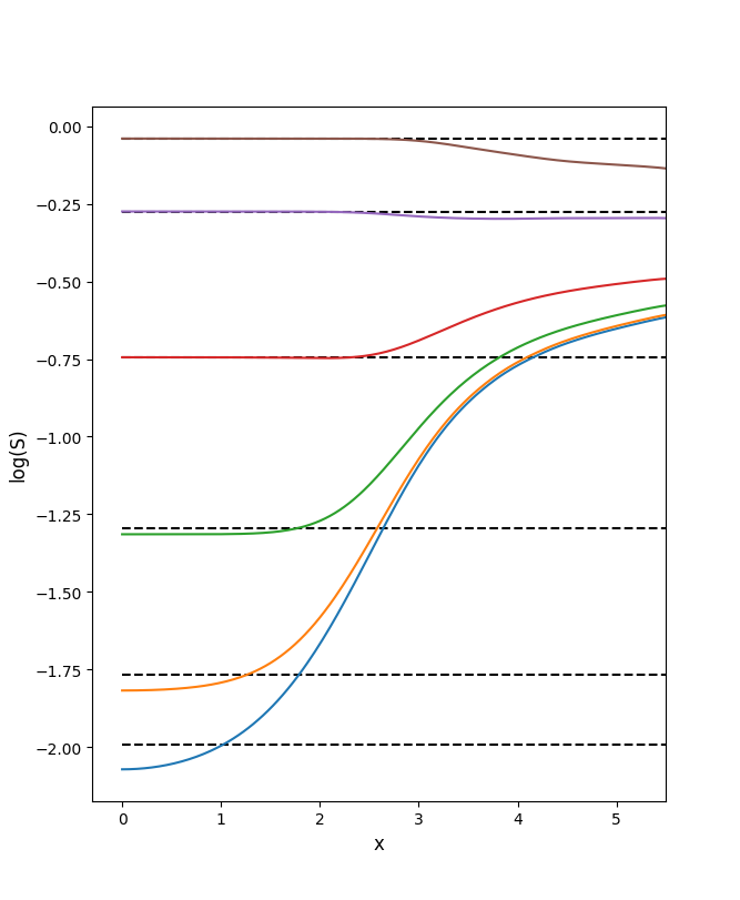
Figure 1: Variation with frequency of the normalized source function, for different values of the optical depth at line center across the atmosphere. Dashed lines indicate the (constant with frequency) CRD values at $\tau=0,\,1,\,10,\,100,\,10^{3},\,10^{4}$ for comparison, where both $S_{\rm CRD}$ and $S(x=0)$ increase with $\tau$. It satisfactorily reproduces the standard PRD results using Hummer’s $R_{\rm I-A}$ (see also Hummer 1969, Fig. 1c).

VI Benchmarking against Hummer’s $R_{\rm I-A}$

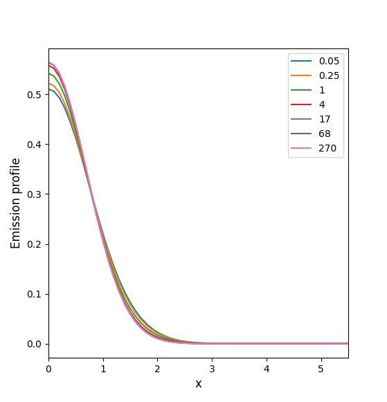
Figure 2: Dependence of the emission profiles $\psi(x,\tau)$ on various optical depths across the atmosphere (see the top-right frame giving the correspondence between $\tau$ at line center and the color of the relevant profile). This distribution is computed self-consistently with the radiation, without the need of any a priori given redistribution function.

Our first task then has been to reproduce the $S(x,\tau)$ results of the original Hummer (1969; his Fig. 1c) publication. It is an obvious comparison to be made, which was not conducted in earlier studies. They were obtained for a 1D, semi-infinite, plane parallel atmosphere of total optical thickness at line center $\tau=10^{6}$, $\varepsilon=10^{-4}$ and $\zeta=0$. In our computations, we used 5 points per decade in order to cover this range. Our solutions for $S(x,\tau)$ are displayed in Fig. (1) where increasing values around line core ($|x|<2$) correspond to successive optical depths of the order of: $\tau=0,\,1,\,10,\,100,\,10^{3},\,10^{4}$. Successive dashed lines mark the (frequency independent) CRD values at the same optical depths, for comparison.

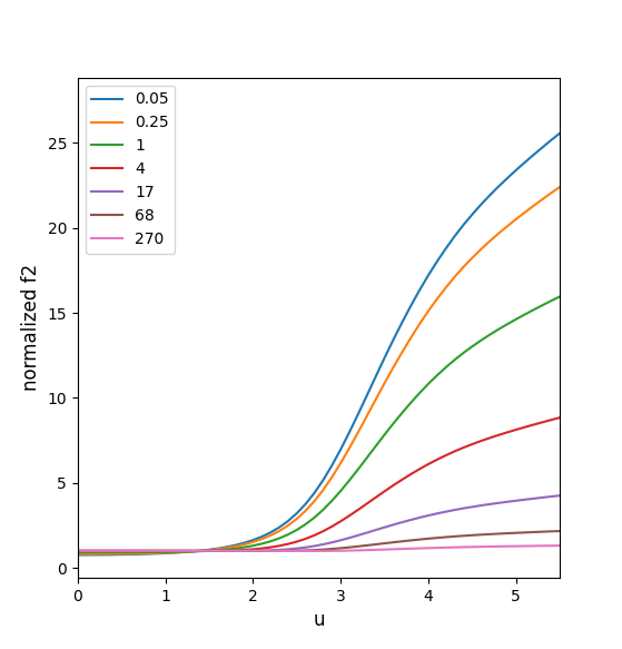
Figure 3: Deviations from Maxwellian illustrated by ratios $f_{2}(u,\tau)/f^{M}(u)$ at various optical depths across the atmosphere using the same convention as in Fig. (2). It shows the “overpopulation” of $f_{2}$ at large $u$’s. This very information cannot be accessed to, using standard non–LTE approaches.

Even using our simple iterative scheme, we recover easily the Hummer (1969) “historic” solutions. We could also check that the relative error on $S(x,\tau)$ between our new scheme vs. similar results obtained with a “frequency by frequency” (hereafter FBF; see Paletou & Auer, 1995) for $R_{\rm I-A}$ never exceeds 4% with a more typical mean value around 1.3% (for this validation, we used FBF with a 6-node Gauss-Legendre angular quadrature).

To achieve this level of accuracy, we compute the CRD solution using the ALI-iteration until the maximum relative error on the source function was better than $10^{-4}$. The new cycle was then iterated up to a maximum relative error on the frequency dependent source function of $3\times 10^{-4}$.

In Fig. (2), we display the emission profile $\psi(x,\tau)$ for different optical depths $\tau$ across the atmosphere. These are “naturally” computed using our approach, and without the need of any a priori given redistribution function. The only assumptions we rely on are: (1) that the VDF $f_{1}$ of the atoms in their ground state is Maxwellian, and (2) that the atomic absorption profile is a priori given, in the present case of coherent scattering by a Dirac function centered at the frequency $\nu_{0}$ of the model-spectral line. Then all relevant quantities, down to the velocity distribution function of the excited atoms at every depth into the atmosphere, are computed consistently with the successive evaluation of the radiation field.

Indeed, we can display, as shown in Fig. (3) a more original sample of the ratios $f_{2}(u,\tau)/f^{M}(u)$ for different optical depths, as considered in Fig. (2). In the present paper, we consider the emission profile $\psi(x,\tau)$ and thereby the source function $S(x,\tau)$ to be independent of the polar angles of the radiation field. Therefore, we prefer to illustrate the normalized VDF of the excited atom that depends only on the modulus of velocity $u$. This is obtained by integrating $f(\vec{u},\tau)$ given by Eq. (3) over atomic velocity directions, namely $d\Omega_{u}$. Important deviations from Maxwellian can be identified, typically for $u>2$, and close to the non-illuminated surface of the semi-infinite atmosphere. We recover easily, using our new numerical procedures, the “overpopulation” of $f_{2}$ at large $u$’s already put in evidence by Borsenberger et al. (1987).

Such a material is only accessible using the Oxenius-like formalism that we adopted. Note also that the de facto neglected potential effects of velocity-changing elastic collisions can only be addressed, and studied in that theoretical frame (see details in PP21 and §7 hereafter). More generally, such additional information could be very valuable for the detailed coupling between the radiation transfer problem and any other physical processes that would take place within an atmosphere, and for which the very knowledge of the various VDF’s of contributing elements, at different excitation and ionization stages would be critical.

VII Non-zero velocity-changing elastic collisions

To the best of our knowledge, such preliminary computations were only addressed by Atanackovi$\check{\rm c}$ et al. (1987) so far.

We now go a bit further by illustrating in Fig. (4) the dependence of the source function at $\tau\approx 1$ on the velocity-changing elastic collisions parameterized as $\zeta$. The model-atmosphere used for this computation is identical to the one adopted in §6, but we have made vary $\zeta$ from $0$ to $50$. As expected, the source function $S(x,\tau)$ ranges between the standard PRD-$R_{\rm I-A}$ solutions when $\zeta=0$, and the frequency independent CRD values (shown as black dashed line) for increasing values of $\zeta$.

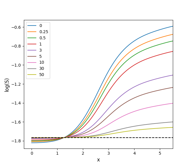
Figure 4: Variation with frequency of the normalized source function at $\tau\approx 1$, for different values of the velocity-changing elastic collision parameter $\zeta$ (indicated in the top-left frame). The model-atmosphere is the same as the one considered in §6 and Hummer (1969). As expected, successive solutions range between standard PRD-$R_{\rm I-A}$ values (blue) and the limit of the CRD solution (dashed line) for increasing values of $\zeta$.

As also expected, the numerical problem becomes easier for increasing values of $\zeta$. Effects of velocity-changing elastic collisions will be discussed in more details in another devoted study.

VIII A finite slab case

Among numerous applications, we are particularly interested in the radiative modelling of isolated and illuminated finite slabs. As an example of expected effects, we simulated a 1D plane parallel horizontal slab strongly irradiated asymmetrically, only from below. This mimics the radiative modelling of a “cold filament” suspended above a stellar disk (see e.g., Paletou 1997).

We used a 33 points optical depth grid, logarithmically spaced away from both open surfaces (using an initial $\delta\tau=0.01$), and symmetric around a midslab depth set at $\tau_{1/2}=500$. For this example we also set $\varepsilon=10^{-4}$ and $\zeta=0$. External illumination is applied only at the bottom surface, using a flat profile of normalized intensity $I_{\rm ext.}=3$.

Figure (5) displays values of the normalized VDF $f_{2}(u,\tau)/f^{M}(u)$ for optical depth values, counted from the top surface, of $\tau=0.58$ and $\tau=1.15$ i.e., around the critical value of 1, and at midslab. The quite strong external illumination that we applied generates very significant departures of $f_{2}$ from Maxwellian, especially at $u>2$ again, but larger than what we already identified for the semi-infinite atmosphere case.

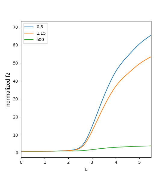
Figure 5: Deviations from Maxwellian illustrated by the changes of the normalized $f_{2}$ at various optical depths (mentioned in the top-left frame) across an asymmetrically and strongly illuminated finite slab of total depth $\tau=10^{3}$. Largest amplitudes are for these two values around $\tau=1$, while smaller but significant deviations are still noticeable at midslab ($\tau=500$).

IX Discussion and conclusion

A first critical evaluation of new numerical procedures in radiative transfer for the solution of the “full non–LTE” problem have been conducted. They were validated by reproducing both CRD and standard PRD with Hummer’s $R_{\rm I-A}$ (Hummer 1962, 1969). This will allow us to now move forward in several directions.

After the very first computations shown here, we shall also be able to evaluate further, in more details, the additional effects of potential velocity-changing elastic collisions with different set of “classic” parameters. Also finite slab models, with different conditions of external illumination will be considered. Such cases lead to more significant departures from Maxwellian than what happens for semi-infinite slabs, as indicated by our preliminary filament-like computation. Relevant astrophysical “objects” should range from solar prominences to circumstellar environements for instance.

The next obvious step is to modify the atomic absorption description for the more realistic case of natural broadening of the upper level of the transition. It would go beyond the previous studies of Borsenberger et al. (1987) and Atanackovi$\check{\rm c}$ et al. (1987) which were limited to “pure” Doppler broadening. Therefore, a Lorentzian profile for atomic absorption will be used. This will also require to implement modifications to the original formalism of Oxenius for that case, following rather Bommier’s (1997) approach, as discussed in PP21. This will be suitable for a preliminary study of resonance lines such as Lyman $\alpha$ of H i for instance. The successive computations of Voigt-like profiles at every iterative step, according to the departures of $f_{2}$ to Maxwellian, and throughout the whole atmosphere will certainly benefit from the numerical scheme proposed by Paletou et al. (2020). This may also require us to implement and validate a more robust iterative scheme, more likely inspired by the so-called FBF scheme proposed by Paletou & Auer (1995).

Then we shall proceed with the consideration of at least an additional distribution, either for another excited state or for free electrons. This should lead to an alternative, less heuristic, approach to the so-called “cross-redistribution” model for the multi-level atoms case (see e.g., Milkey et al. 1975, Hubeny & Lites 1995, Sampoorna & Nagendra 2017).

- (1) Atanackovi, O., Borsenberger, J., Oxenius, J., Simonneau, E. 1987, JQSRT, 38, 427
- (2) Bommier, V. 1997, A&A, 328, 706
- (3) Borsenberger, J., Oxenius, J., Simonneau, E. 1986, JQSRT, 35, 303
- (4) Borsenberger, J., Oxenius, J., Simonneau, E. 1987, JQSRT, 37, 331
- (5) Hubeny, I. & Lites, B. 1995, ApJ, 455, 376
- (6) Hubeny, I. & Mihalas, D. 2014, Theory of Stellar Atmospheres: An Introduction to Astrophysical Non-equilibrium Quantitative Spectroscopic Analysis, Princeton University Press
- (7) Hummer, D.G. 1962, MNRAS, 125, 21
- (8) Hummer, D.G. 1969, MNRAS, 145, 95
- (9) Lambert, J., Paletou, F., Josselin, E., Glorian, J.-M. 2016, Eur. J. Phys, 37, 015603
- (10) Milkey, R.W., Shine, R.A., Mihalas, D. 1975, ApJ, 199, 718
- (11) Oxenius, J. 1986, Kinetic theory of particles and photons – Theoretical foundations of non–LTE plasma spectroscopy, Springer
- (12) Paletou, F. 1997, A&A, 317, 244
- (13) Paletou, F., Auer, L.H. 1995, A&A, 297, 771
- (14) Paletou, F., Bommier, V., Faurobert, M. 1999, in Solar polarization, K.N. Nagendra and J.O. Stenflo eds., Kluwer
- (15) Paletou, F., Peymirat, C. 2021, A&A, 649, A165
- (16) Paletou, F., Peymirat, C., Anterrieu, E., Böhm, T. 2020, A&A, 633, A111
- (17) Sampoorna, M., Nagendra, K.N. 2017, ApJ, 838, 95
- (18) Sampoorna, M., Nagendra, K.N., Frisch, H. 2011, A&A, 527, A89