Climbing the Cliffs: Classifying YSOs in the Cosmic Cliffs using a ML Approach with JWST Data

Abstract

The James Webb Space Telescope (JWST) observed a section of the star forming region NGC 3324 during its Early Release Observations. We make use of the Probabilistic Random Forest machine learning model to identify YSOs within the field of view. We build a matched catalog from photometry data products available on the Mikulski Space Telescope Archive and retrieve 8632 objects, of which Spitzer previously detected 458. We use previously classified data from Spitzer to train on a sample of the Webb data. We retrieve a total of 72 YSO candidates within the data field, 52 of which are only visible with JWST.

1 Introduction

On July 11th, 2022, the first observations from the James Webb Space Telescope (JWST) were released (Pontoppidan et al., 2022). These data included observations of four different astrophysical objects, one of which was the NGC 3324 star-forming region located adjacent to the Carina Nebula. JWST imaged NGC 3324 with two instruments: the Near Infra-Red Camera (NIRCam) to observe the dust collections and look for emission lines of H₂, Poly-Aromatic Hydrocarbons (PAHs) and Pa-$\alpha$; and the Mid Infra-Red Instrument (MIRI) which was able to probe for objects hidden within the dust that may have been rendered invisible at shorter wavelengths.

Filter	$t_{exp}(s)$	Use
F090W	25768.32	dust and background stellar field
F187N	46382.88	ionized gas via the bright Pa-$\alpha$
F200W	25768.32	dust and background stellar field
F335M	6442.08	3.3 $\mu m$ PAH emission
F444W	6442.08	dust scattering from large grains
F470N	11595.72	H2 from embedded jets/outflows
F770W	6771.08	PAH emission
F1130W	6771.08	PAH emission
F1280W	6993.12	12.81 $\mu m$ [Ne II] line emission
F1800W	5994.08	cool dust and proplyds

Table 1: JWST filters used by ERO to image NGC 3324, their exposure times, and their uses as described in Pontoppidan et al. (2022). The first block lists NIRCam filters and the second lists MIRI filters.

The Early Release Observations (ERO, Pontoppidan et al., 2022) of NGC 3324 focused on a $\sim$7$\farcm$4 $\times$ 4$\farcm$4 area with NIRCam, and a $\sim$6$\farcm$4 $\times$ 2$\farcm$2 area within the NIRCam field with MIRI, relatively small areas in comparison to the entirety of NGC 3324, termed the Cosmic Cliffs (hereafter CC). The data were collected in six NIRCam bands and four MIRI bands; see Table 1 for details on bands used, exposure times, and uses. The exposure times varied for each filter, and the FULLBOX 10-point dither pattern was used for NIRCam imaging and 8-point dither for MIRI imaging (Pontoppidan et al., 2022). The FITS images as well as a source catalog generated for each filter by the JWST pipeline were made publicly available through the Mikulski Archive for Space Telescopes. For our use, we access the source catalogs at MAST created using Source Extractor (SExtractor, Bertin & Arnouts, 1996) as part of the JWST pipelines. These data products were reprocessed since July 2022 as better JWST flux calibrations became available; for this paper, the data products for NGC 3324 were last accessed on December 19th, 2022.

Already, the JWST data of NGC 3324 have been probed to understand the capabilities of JWST to detect jets and outflows. Reiter et al. (2022) looked at the narrowband 1.87 $\mu$m filter and the difference between the narrowband 4.7 $\mu$m and wideband 4.44 $\mu$m filters from JWST. In combination with archival Hubble data, they used this dataset to identify 31 outflows within the field of view, including 7 Herbig-Haro objects only visible in the infrared (IR). Along with their identifications of outflows, they provided a list of 24 possible progenitor Young Stellar Objects (YSOs). These progenitors were determined as IR-excess sources located along the estimated line of travel determined by tracing the outflows back in time. As not all objects were visible in the Hubble data, they did not have proper motions for all outflows, and so straight-line estimation was used when appropriate. Reiter et al. (2022) also checked to see if any of their identified YSO candidates had been previously identified with Spitzer data via comparison with the Spitzer-IRAC Catalog for YSOs (SPICY, Kuhn et al., 2021), a catalog developed with the use of machine learning (ML), and found matches to 6/24 possible progenitors.

1.1 Machine Learning Tools

Within the last several years, ML has emerged as a useful tool within star formation (e.g. Miettinen, 2018; Cornu & Montillaud, 2021; Chiu et al., 2021; Kuhn et al., 2021). These and other works have used Gradient Boosting (Miettinen, 2018), neural networks (Miettinen, 2018; Cornu & Montillaud, 2021; Chiu et al., 2021), and random forest models (Kuhn et al., 2021), among others. Each of these ML approaches have their strengths, and each has successfully separated YSOs from the contaminating classes of stars, galaxies, PAHs, and Active Galactic Nuclei (AGN) to high accuracies.

A common pitfall with ML classification algorithms occurs with imbalanced data-sets. As YSOs are much less frequent than regular field stars, this imbalance is a relevant issue within the star formation field. Random Forest (RF) models are better at handling imbalanced datasets, by individually classifying each object based off of a training set (Breiman, 2001). Kuhn et al. (2021), whose catalog previously included the YSOs within the CC, utilized a RF trained on an imbalanced mix of YSOs and contaminant field objects where the number of YSOs accounted for less than 25% of the full training set. They used the area under the receiver-operator curve as their metric to determine the best fit model. As RF models output the probabilities of objects being in the positive class, Kuhn et al. (2021) chose that an object would be classified as a YSO if it had at least a 50% probability of being so as determined by their singular RF network. After YSOs were identified, Kuhn et al. (2021) further used cuts based on the spectral index to determine the stages of star formation the YSOs are in, labelling them as either Class I, Flat-Spectrum, or Class II YSOs.

A second common issue with ML is that most ML algorithms cannot handle missing data. Kuhn et al. (2021) worked around this issue by using copulas, i.e., functions which connect the probability distributions of different features to each other. When using copulas, the joint probability distributions of the data are decomposed into their marginal components, and the copula couples these probabilities together (Nelsen, 2007). Using copulas to fill missing data, however, assumes that data are missing because an object is not in the field of view of the given filter. Chiu et al. (2021) used a different approach to missing data that assumes objects in question are within the field of view of the filter, but no point sources were detected. Such detection gaps could happen when an object is heavily obscured in certain filters. The solution provided by Chiu et al. (2021) is to fill the data in missing bands with 1% of the smallest flux obtained in that band as a reasonable estimate for the thermal noise of the detector. This method hence accounts for the clarity of an object at different wavelengths, which is important for the determination of class.

An alternative solution to the issue of missing data is provided by the Probabilistic Random Forest (PRF) method released by Reis & Baron (2019), which has successfully been applied to high-mass YSO identification in Local Group galaxies (e.g., Kinson et al., 2021, 2022). The PRF method uses both the values and errors of each filter to create probability distributions for each data point, where the expectation value is the data point’s flux, and the standard deviation is the error on this flux, assuming a Gaussian distribution. An RF-like algorithm is hence trained, and when an object is sent through the network, it is no longer sent along one branch of the tree. Instead, at every decision node, the probability of the object being on either side of the node is propagated, with probability determined by the Gaussian distribution. For a full prescription, see Reis & Baron (2019). This method has the benefit of not assuming what the missing data may be while still accounting for them by passing any node that relies upon the data with equal probability to either side.

Reis & Baron (2019) provide a comparison with the regular RF that shows that when all labels are correct, the PRF and RF perform at the same accuracy. When purposefully introducing incorrect target labels, however, they find that the PRF greatly outperforms the regular RF. We perform our own check of the performance of the PRF vs a regular RF, using both copulas and thermal noise to fill the missing data with the regular RF. To perform a fair comparison, we use data from the Cores to Disks (c2d, Evans et al., 2014) survey, which contains data with both completely filled and missing values. We first use 10 000 objects with all bands available, then 9000 objects with all bands available and an additional 1000 (randomly chosen) objects with data missing in at least one band to obtain a case where 90% of data is filled. Similarly, we also obtain data-sets where 80%, 70%, 60%, and 50% of data are filled. In all cases, the data are real observations, and no data are artificially removed. We use YSOs as our positive class and all others as contaminants, where YSOs make up approximately 1/3 of the sample. Figure 1 shows the performance in all three cases with a decrease in available data. We find that all three cases perform within a few percent. In general, filling the data with noise and using copulas perform equally well. We use the Python package copulas for our calculations.

Figure 1: A comparison of the F1-Scores for the validation set of the PRF (solid red line), RF filled via copulas (blue dashed line), and RF filled with thermal noise (purple dashed line) as a function of the amount of missing data.

This Letter is split into the following sections. Section 2 describes how we created the catalog of JWST data for NGC 3324, as well as a description of the ML model used. Section 3 provides the results of this ML model, including the number of candidate YSOs detected and a comparison with those found by both Kuhn et al. (2021) and Reiter et al. (2022). Finally, Section 4 discusses the accuracies of our classification, and provides an analysis of the capabilities of JWST for YSO detection in comparison to Spitzer.

2 Methodology

2.1 Catalog Creation

The data retrieved from MAST were available as the direct outputs from SExtractor (Bertin & Arnouts, 1996), which provided both fluxes and magnitudes, as well as sizes and locations, for all of the point sources detected within a given filter. To match objects between filters, we find those objects whose equatorial coordinates are within one sigma of the center of the source, as determined by SExtractor in F470N-F444W. Because of JWST’s extraordinary resolution, this matching criterion remains a very small solid angle, ensuring each object is correctly linked across wavelengths. We used the Astropy (The Astropy Collaboration et al., 2018) match_coordinates_sky_ task to build our catalog of objects in all bands. We removed all objects which contained only one data-point after catalog matching was completed. This approach resulted in a total of 8632 individual point sources.

We next used the Astropy (The Astropy Collaboration et al., 2018) match_coordinates_sky_ task to match the Spitzer detections from the GLIMPSE catalog (Preibisch et al., 2014) and available SPICY targets (Kuhn et al., 2021). Again, matches were identified when objects were within one sigma of the JWST source, resulting in 458 objects detected by both Spitzer and JWST, 26 of which were labelled as YSOs with SPICY (Kuhn et al., 2021).

The MAST SExtractor files provided both variable aperture and isophotal photometry for each point source. To identify the best type of photometry to use, we compared the photometry of sources matched in both the JWST 4.44 $\mu$m and Spitzer 4.5 $\mu$m bands, whose transmission curves are very similar. As such, we expect that flux values in these two bands should be very similar. We find that the isophotal photometry best approaches a 1:1 correlation between these two bands, and thus our final catalog uses only isophotal photometry for JWST data.

2.2 Applying the Probabilistic Random Forest method

To classify the full JWST dataset, we must first have predetermined classifications for some portion of the data. The SPICY catalog (Kuhn et al., 2021) provided classifications of all YSOs within the GLIMPSE survey, of which NGC 3324 was included. After retrieving the GLIMPSE catalog, and matching it to the SPICY targets, we were able to say that any object not classified as a YSO by SPICY was then classified as a contaminant (Kuhn et al., 2021), and so we obtained classifications for all objects detected in the Spitzer IRAC bands for the CC. The cross-matched catalogue became the training set for classifying further JWST data within the CC field of view. By training on data within this field, the possible effects of extinction on the measured fluxes are eliminated. Furthermore, the absolute flux calibration is less important that the shape of the spectrum as it the latter is what the model learns.

The very dusty field of the CC means there are many objects within it that are not visible at all wavelengths. We hence choose to use the probabilistic random forest (PRF) method for our classification. The PRF requires three input parameters for supervised classification: the input data, errors on the input data, and the targets for the input data. We test several different input data structures: including all ten bands available, removing only the narrow bands, removing only the MIRI bands, and finally removing one band at a time to test for improvements within the classification. In all cases, our training set is then made up of 25% YSOs and 75% contaminant objects. Our validation set was the entire set of previously classified objects.

To determine the best configuration of the PRF, we ran the model 500 times, changing the random seed between 0 and 1000. There are four possible metrics we could have chosen from: accuracy, recall, precision, and F1-Score. Each of these metrics requires some combination of the numbers of True Positives (TP), False Positives (FP), True Negatives (TN), and False Negatives (FN). For our case, TP is the number of objects correctly classified as YSOs, TN is the number of objects correctly classified as contaminants, FP is the number of contaminant objects incorrectly classified as YSOs, and FN is the number of YSOs incorrectly classified as contaminants. Accuracy, $A=(TP+TN)/(TP+FP+FN+TN)$ is a measure of the total number of correct identifications but can be easily made suspiciously high as a result of a much larger negative class. As such, we do not use it as our metric. The F1-score, $F1=2R\times P/(R+P)$, however, is a metric defined as the harmonic balance between recall $R=TP/(TP+FN)$ and precision $P=TP/(TP+FP)$. We use it as our metric of choice because we wish to obtain a network with low contamination by much more numerous stars (high precision) while still maintaining a high recovery of YSOs (high recall).

Along with providing classifications, the PRF also allows us to determine which bands are most important to the classification and which bands, if any, are superfluous through the PRF feature_importances_ method. To determine the order of importance, the most important band is successively removed from the data input ensemble, and the classification is repeated until no bands are left. Table 2 lists the bands from most important to least important, the F1-scores for both the training and validation sets when only that band is removed, and the number of YSOs found in the full JWST dataset of 8632 objects.

Band	F1 % (tr)	F1 % (va)	# YSOs
F470N	84	72	63
F444W	82	68	107
F335M	84	73	73
F187N	84	75	90
F090W	94	75	95
F200W	92	67	985
F1280W	82	72	72
F1130W	82	71	99
F770W	87	75	97
F1800W	84	72	149
All bands present	84	72	141
N bands removed	82	71	62
MIRI bands removed	84	75	126

Table 2: The bands are listed from from most to least important for YSO identification as determined using the PRF feature_importances_ tool. In each column, the band in that row is removed, and the metrics are calculated. F1-Scores are given for the training and validation sets in the first and second columns, respectively. F1-Scores have an error of $\sim 2\%$. The number of YSOs found in the full JWST dataset are labelled in the last column.

The number of YSOs identified is seen to vary based on the classification, despite the F1-Scores remaining similar. Indeed, when we randomly seed the PRF 1000 times we find that $\sim$60% of the time, less than 100 objects out of 8632 are classified as YSOs. Figure 2 shows the distribution of the number of objects classified as YSOs compared to the F1-Scores for each run. Hence, we take the classifications for all objects over 1000 runs of the model and take the probability of a given object being a YSO as the fraction of times that it is identified as a YSO. As in Kuhn et al. (2021), if a given object has a probability of greater than 50%, then it is classified as a YSO. Figure 3 shows various metrics for the validation set of the YSO classification as a function of the cut on the probability of a given object being a YSO. The higher the cut, the fewer objects are classified as YSOs, leading to a decrease in recall and increase in precision, though the F1-Score remains relatively even. At around a cut of 40%, the precision, recall, and F1-Score are nearly equivalent. There are no YSOs with 100% probability, leading to the sharp decrease in all metrics at this cut. The figure confirms that 50% is a reasonable cut for the probability of the object being a YSO.

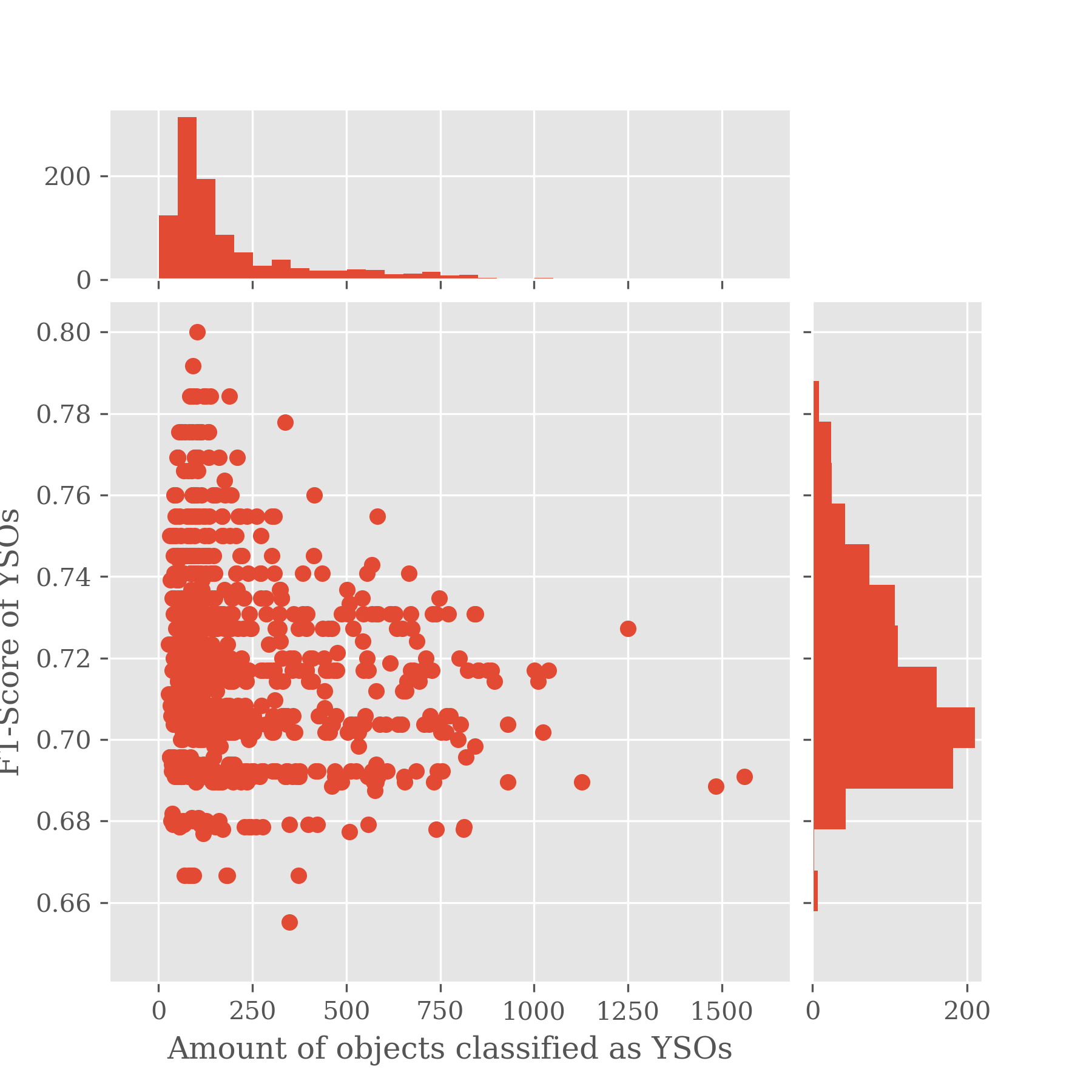
Figure 2: A plot comparing the number of YSOs found vs the F1-Score on the validation sets for 1000 runs of the PRF using all JWST bands available.

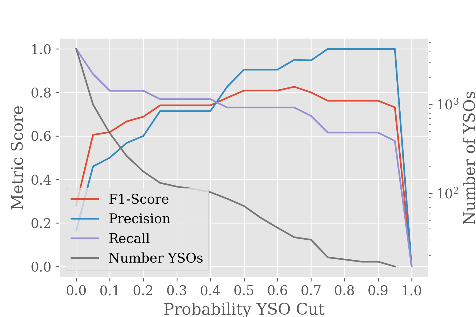
Figure 3: The trends of various metrics with a variation of the cut in probability that determines if a given object is a YSO. The number of YSOs returned dependant on this probability. There are no YSOs with 100% probability.

3 Results

From the JWST photometry of CC, we retrieve a total of 8632 objects. Only 72 of these objects are found to be YSOs, with a probability greater than 50%. Of these, 20 were recovered from the 26 SPICY objects, leading to a recall of 73%, precision of 90%, and an F1-Score of 81%. We also find that of the 23 candidate progenitors identified in Reiter et al. (2022) only three, previously identified in SPICY (Kuhn et al., 2021), were found to be YSOs in our final classification.

While analyzing the feature_importances_, it is expected that if all features (filters) are independent, the importance of each band will remain the same even as other bands are taken away. In the case where two bands switch position in the order of feature_importance_ these bands are correlated. Some correlation is apparent between F770W, F1280W, and F1800W, as these three bands routinely shifted ordering when determining the band importance. Similarly, F090W and F200W were found to be slightly correlated by this method. The narrow bands F187N and F470N, which trace Pa-$\alpha$ and H₂ emission, respectively, were not found to be especially important for classification. Removing one or the other did not greatly impact the classification, nor did the removal of both filters data. In general, any one band can be removed without a great impact on the F1-Score.

Similarly, MIRI bands were not found to be especially influential to the classification, although this is likely due to the unavailability of data for nearly half the field of view imaged by NIRCam. Furthermore, we were only able to train on objects with Spitzer IRAC data; for those objects whose SEDs peak within the mid- to far-infrared they may not be sampled in the training set, whose JWST SEDs will follow the Spitzer SEDs. This potential bias will hopefully be eliminated in future work.

We found that, out of the 458 objects classified by SPICY in the CC, 418 were consistently classified by both us and SPICY. Unsurprisingly, we found that the objects not consistently classified between our approach and that of SPICY tend to have fewer bands available. In particular, there were two objects which were classified as YSOs in SPICY but as contaminants in our work, and they both contain data in only three out of ten bands. Indeed, this behaviour may be biased by the match between Spitzer and JWST data, where the locations of the Spitzer point sources may have been closer to a different point source in JWST data, an effect caused by the lower resolution of Spitzer in comparison to JWST. Similarly, objects classified as contaminants in SPICY and YSOs in our work tend to be missing the 4.44 $\mu$m and 4.70 $\mu$m JWST photometry, while their proposed Spitzer counterparts contain data in this range. One of the SPICY YSOs is only captured in the MIRI data as it is offset from the NIRCam data.

4 Discussion and Conclusion

This work aimed to provide classifications of YSOs within the ERO JWST data of NGC 3324. There are $\sim 8600$ objects within the JWST fields of $\sim 7.4^{\prime}\times 4.4^{\prime}$ by NIRCam and $\sim 6.4^{\prime}\times 2.2^{\prime}$ by MIRI. Of these objects, less than 500 were detectable by Spitzer. Those that were detectable were classified and made available as a catalog (SPICY) by Kuhn et al. (2021). We match the SPICY catalog to the GLIMPSE data (Preibisch et al., 2014) so that we have a record of the objects which are contaminants or YSOs. The classified population within the CC fields then made up our training set for our probabilistic random forest model to classify JWST data.

With our small training set, it is very possible to have overfit our model to the available data. We do see that the training set performs around 10% better, a key signpost of overfitting. However we do see a similar trend between the training and validation sets as we modify the input data, suggesting that the issue is not as severe.

With even this small amount of classified data, we were able to separate 72 YSO candidates from the rest of the JWST data. Table 3 contains a comparison of the objects labelled by Reiter et al. (2022) and Kuhn et al. (2021) as well as those objects we newly identify as YSO candidates. We recover 20/26 SPICY YSOs, i.e. approximately a 73% recall rate.

The YSOs identified in SPICY are estimated to have a less than 10% contamination rate (Kuhn et al., 2022). Of the seven objects identified as contaminants in our algorithm, one of them was mismatched, and one of them is only available in MIRI data. Of the remaining five, three have a probability of being a YSO less than 10%. As such, 3/26 objects give a contamination rate of 11.5%, which is similar to the 10% contamination rate identified in Kuhn et al. (2022) over an analysis of 26 YSO candidates.

JWST Number	Kuhn et al. (2021)	This work
J103635.2-584029	CI - SPICY 7409
J103648.7-583803	CII - SPICY 7428	YSO
J103652.5-583725	CI - SPICY 7435	YSO
J103656.6-583659	CII - SPICY 7444	YSO
J103657.4-583637	CII - SPICY 7447	YSO
J103658.4-583619	FS - SPICY 7448	YSO
J103658.9-583742	CII - SPICY 7452
J103659.1-583524	FS - SPICY 7454	YSO
J103700.1-583528	FS - SPICY 7461	YSO
J103700.4-583829	CII - SPICY 7462	YSO
J103700.7-583545	CII - SPICY 7464	YSO
J103700.8-583622	FS - SPICY 7465	YSO
J103702.5-583403	CI - SPICY 7469	YSO
J103705.7-583418	FS - SPICY 7473	YSO
J103706.4-583517	CII - SPICY 7475	YSO
J103706.7-583419	CII - SPICY 7476	YSO
J103706.9-583655	CII - SPICY 7477	YSO
J103708.4-583654	CII - SPICY 7479	YSO
J103711.3-583445	CII - SPICY 7481	YSO
J103711.7-583424	CII - SPICY 7482
J103642.3-583804	-
J103648.0-583819	-
J103647.3-583810	CI - SPICY 7423	YSO
J103646.7-583805	-
J103651.5-583754	-
J103650.5-583752	-
J103651.4-583748	-
J103653.8-583748	-
J103651.5-583710	-
J103654.2-583626	-
J103654.4-583618	-
J103654.0-583720	CI - SPICY 7441
J103653.6-583520	-
J103653.1-583737	-
J103653.3-583754	UN - SPICY 7438	YSO
J103652.7-583805
J103653.1-583708	-
J103651.6-583658	-
J103652.3-583809	CI - SPICY 7434
J103653.9-583629	FS - SPICY 7440
J103701.5-583751	-
J103702.1-583658	CII - SPICY 7467	YSO
J103653.9-583632	-

Table 3: The top half of this table shows the YSOs identified with Kuhn et al. (2021) and whether or not they were classified as YSOs with our model. Classes are included as CI = Class I, CII = Class II, FS = Flat Spectrum, and UN = Uncertain for those objects found within Kuhn et al. (2021). The bottom half of this table shows the objects identified by Reiter et al. (2022) as potential progenitors for jets and the comparable YSO candidates within this work and Kuhn et al. (2021).

At this stage, we obtained a high F1-Score for the validation set, and we can assume a low contamination based off of the number of YSOs that we retrieved from the full dataset of 8632 objects. If even 10% of contaminants were misclassified as YSOs, we would have greater than 800 objects classified as YSOs. As it is, by bootstrapping the results, we obtained the probability of an object being a YSO based off the number of times it was classified by a PRF (whose validation F1-Score was approximately 81%). We report an object as a YSO if the probability of being a YSO is greater than the probability of being a contaminant (50%). We include the probabilities in our published catalog for future reference.

Based upon these probabilities, we find that the PRF method (Reis & Baron, 2019) holds promise for accurate YSO identification from JWST data, especially as we wait for more data to become available. At this stage, we are limited by the relatively small amount of previously classified data available. We cannot yet, for instance, realistically apply the ML model to determine the stage of star formation. The PRF, however, was able to recover previously identified YSOs to 85% F1-Score and retrieved a reasonable number of YSOs from the entire set. With more JWST data becoming available and the use of synthetic JWST data, these metrics can only improve.

References

- Bertin & Arnouts (1996) Bertin, E., & Arnouts, S. 1996, A&AS, 117, 393, doi: 10.1051/aas:1996164
- Breiman (2001) Breiman, L. 2001, Machine Learning, 45, 5, doi: 10.1023/A:1010933404324
- Chiu et al. (2021) Chiu, Y. L., Ho, C. T., Wang, D. W., & Lai, S. P. 2021, Astronomy and Computing, 36, 100470, doi: 10.1016/j.ascom.2021.100470
- Cornu & Montillaud (2021) Cornu, D., & Montillaud, J. 2021, A&A, 647, A116, doi: 10.1051/0004-6361/202038516
- Evans et al. (2014) Evans, N. J., I., Allen, L. E., Blake, G. A., et al. 2014, VizieR Online Data Catalog, II/332
- Kinson et al. (2021) Kinson, D. A., Oliveira, J. M., & van Loon, J. T. 2021, MNRAS, 507, 5106, doi: 10.1093/mnras/stab2386
- Kinson et al. (2022) —. 2022, MNRAS, 517, 140, doi: 10.1093/mnras/stac2692
- Kuhn et al. (2021) Kuhn, M. A., de Souza, R. S., Krone-Martins, A., et al. 2021, ApJS, 254, 33, doi: 10.3847/1538-4365/abe465
- Kuhn et al. (2022) Kuhn, M. A., Saber, R., Povich, M. S., et al. 2022, AJ, 165, 3, doi: 10.3847/1538-3881/ac9314
- Miettinen (2018) Miettinen, O. 2018, Ap&SS, 363, 197, doi: 10.1007/s10509-018-3418-7
- Nelsen (2007) Nelsen, R. B. 2007, An introduction to copulas (Springer Science & Business Media)
- Pontoppidan et al. (2022) Pontoppidan, K. M., Barrientes, J., Blome, C., et al. 2022, ApJ, 936, L14, doi: 10.17909/67ft-nb86
- Preibisch et al. (2014) Preibisch, T., Zeidler, P., Ratzka, T., Roccatagliata, V., & Petr-Gotzens, M. G. 2014, A&A, 572, A116, doi: 10.1051/0004-6361/201424045
- Reis & Baron (2019) Reis, I., & Baron, D. 2019, PRF: Probabilistic Random Forest, Astrophysics Source Code Library, record ascl:1903.009. http://ascl.net/1903.009
- Reiter et al. (2022) Reiter, M., Morse, J. A., Smith, N., et al. 2022, MNRAS, doi: 10.1093/mnras/stac2820
- The Astropy Collaboration et al. (2018) The Astropy Collaboration, Price-Whelan, A. M., Sipőcz, B. M., et al. 2018, AJ, 156, 123, doi: 10.3847/1538-3881/aabc4f