Spectral form factor in the $\tau$-scaling limit

Abstract

We study the spectral form factor (SFF) of general topological gravity in the limit of large time and fixed temperature. It has been observed recently that in this limit, called the tau-scaling limit, the genus expansion of the SFF can be summed up and the late-time behavior of the SFF such as the ramp-plateau transition can be studied analytically. In this paper we develop a technique for the systematic computation of the higher order corrections to the SFF in the strict tau-scaling limit. We obtain the first five corrections in a closed form for the general background of topological gravity. As concrete examples, we present the results for the Airy case and Jackiw-Teitelboim gravity. We find that the above higher order corrections are the Fourier transforms of the corrections to the sine-kernel approximation of the Christoffel-Darboux kernel in the dual double-scaled matrix integral, which naturally explains their structure. Along the way we also develop a technique for the systematic computation of the corrections to the sine-kernel formula, which have not been fully explored in the literature before.

1 Introduction

Spectral form factor (SFF) is a useful measure of the level statistics of quantum chaotic systems sff and it is widely studied in many areas of physics. In the context of quantum gravity and holography, the SFF of the Sachdev-Ye-Kitaev (SYK) model Sachdev1993 ; Kitaev1 ; Kitaev2 was studied in Garcia-Garcia:2016mno ; Cotler:2016fpe as a useful diagnostics of the Maldacena’s version of the information problem Maldacena:2001kr . It is found that the SFF of the SYK model exhibits the behavior of the ramp and plateau as a function of time, which is consistent with the conjecture that the level statistics of quantum chaotic system is universally described by a random matrix model bohigas1984 . As shown in Saad:2019lba , Jackiw-Teitelboim (JT) gravity Jackiw:1984je ; Teitelboim:1983ux , which is holographically dual to the low energy sector of the SYK model, is indeed described by a certain double-scaled random matrix model. In the bulk gravity picture, the ramp of the SFF of JT gravity comes from the contribution of a wormhole connecting two boundaries of spacetime Saad:2018bqo . In the matrix model picture, it is described by the connected part of the correlator of two macroscopic loop operators Banks:1989df . On the other hand, the plateau of the SFF is very mysterious from the viewpoint of bulk gravity and it was speculated that the appearance of the plateau is related to some non-perturbative effects in quantum gravity Cotler:2016fpe ; Saad:2019lba . In the matrix model picture, it is argued in Cotler:2016fpe ; Saad:2019lba that the plateau can be explained by the Andreev–Altshuler instantons andreev1995spectral . See also Okuyama:2018gfr for an explanation of the plateau by eigenvalue instantons.

In this paper, we will consider the connected part of the SFF in 2d quantum gravity

$$\text{SFF}=\langle Z(\beta+\mathrm{i}t)Z(\beta-\mathrm{i}t)\rangle_{\rm c},$$ (1)

where $Z(\beta)=\operatorname{Tr}e^{-\beta H}$ and the expectation value is defined by averaging over a random matrix $H$. As shown in Brezin:1990rb ; Douglas:1989ve ; Gross:1989vs , 2d quantum gravity coupled to a conformal matter can be defined by a certain double-scaling limit of a random matrix model. More generally, one can introduce couplings $\{t_{k}\}\ (k=0,1,2,\ldots)$ to the matrix model potential. Then the free energy of the model is interpreted as a generating function of the intersection numbers on the moduli space of Riemann surfaces and the model is called topological gravity Witten:1990hr . There is an underlying integrable structure in this model and the free energy serves as a tau-function of the KdV hierarchy Witten:1990hr ; Kontsevich:1992ti . It turns out that the matrix model of JT gravity in Saad:2019lba is a special case of topological gravity where infinitely many couplings $\{t_{k}\}$ are turned on in a specific way mulase ; Dijkgraaf:2018vnm ; Okuyama:2019xbv and it corresponds to the computation of Weil-Petersson volumes mirzakhani2007simple ; Eynard:2007fi .

SFF exhibits the ramp-plateau transition around the time scale $t\sim\hbar^{-1}$, called the Heisenberg time, where $\hbar$ is the genus-counting parameter of the matrix model. Recently, it is observed in Saad:2022kfe ; Blommaert:2022lbh ; Weber:2022sov that one can focus on the ramp-plateau transition regime by taking what is called the “$\tau$-scaling limit”

$$t\to\infty,\quad\hbar\to 0,\quad\tau=t\hbar:\text{fixed},$$ (2)

with $\beta$ fixed in (1). In this limit, SFF is expanded as

$$\text{SFF}=\sum_{g=0}^{\infty}\hbar^{2g-1}\text{SFF}_{g}(\tau,\beta).$$ (3)

Remarkably, it is found that the leading term $\text{SFF}_{0}$ can be computed in a closed form by just summing over the original genus expansion in the $\tau$-scaling limit and the resulting $\text{SFF}_{0}$ approaches a constant as $\tau\to\infty$ Saad:2022kfe . This opens up an interesting avenue for a “perturbative plateau.”

In this paper, we will develop a technique for the systematic computation of the higher order corrections $\text{SFF}_{g}~{}(g\geq 1)$. By using our method, we obtain $\text{SFF}_{g}$ up to $g=5$ for arbitrary couplings $\{t_{k}\}$ of topological gravity. It turns out that $\text{SFF}_{g}$ has a structure which is a natural generalization of $\text{SFF}_{0}$. In Saad:2022kfe it was shown that $\text{SFF}_{0}$ is essentially determined by the Fourier transform of the universal part of the two-body eigenvalue correlation, known as the sine kernel formula Gaudin:1961 ; Dyson:1962es ; Brezin:1993qg . We find that the higher order correction $\text{SFF}_{g}$ is closely related to the correction of the Christoffel-Darboux (CD) kernel to the naive sine kernel formula. Rather surprisingly, such corrections to the sine kernel formula have not been fully explored in the literature before, as far as we know. We will also develop a technique for the systematic computation of the corrections of the CD kernel and confirm that $\text{SFF}_{g}$ is correctly reproduced form the Fourier transform of the CD kernel by including the corrections to the sine kernel formula.

This paper is organized as follows. In section 2, we review the known results about the SFF in the $\tau$-scaling limit. Along the way we consider the $\tau$-scaling limit based on the genus expansion of the SFF and obtain the small $\tau$ expansion of $\text{SFF}_{g}$ for small $g$. In section 3, we summarize our results of $\text{SFF}_{g}$ and the higher order corrections of the CD kernel. We also explain their relations. In section 4, based on our general results we compute $\text{SFF}_{0}$ and $\text{SFF}_{1}$ for the Airy case and JT gravity, as concrete examples. In section 5, we formulate a systematic method of computing $\text{SFF}_{g}$. In section 6, we explain how to compute the higher order corrections of the CD kernel beyond the sine kernel approximation. Finally we conclude in section 7. In Appendix A, we compute the corrections of the Airy kernel to the sine kernel formula. In Appendix B, we present an explicit form of the coefficient that determines $\text{SFF}_{2}$.

2 $\tau$-scaling limit of SFF

In this section we will briefly review the known results about the SFF in the $\tau$-scaling limit. We will consider the $\tau$-scaling limit for the general background of topological gravity based on the known genus expansion of the SFF, which enables us to compute the small $\tau$ expansion of $\text{SFF}_{g}$ for small $g$.

For the general background $\{t_{k}\}$ of topological gravity, the connected two-boundary correlator is expanded as Okuyama:2020ncd

$$\langle Z(\beta_{1})Z(\beta_{2})\rangle_{\rm c} =\frac{\sqrt{\beta_{1}\beta_{2}}}{2\pi}e^{-(\beta_{1}+\beta_{2})E_{0}}\Biggl{[}\frac{1}{\beta_{1}+\beta_{2}}$$ (4)

$$\qquad+\left(\frac{\beta_{1}^{2}+\beta_{1}\beta_{2}+\beta_{2}^{2}}{24s^{2}}+\frac{2(\beta_{1}+\beta_{2})I_{2}+I_{3}}{24s^{3}}+\frac{I_{2}^{2}}{12s^{4}}\right)g_{\rm s}^{2}+\mathcal{O}(g_{\rm s}^{4})\Biggr{]},$$

where $g_{\rm s}$ is the genus-counting parameter related to $\hbar$ as

$$g_{\rm s}=\sqrt{2}\hbar.$$ (5)

$I_{k}$ denote the Itzykson-Zuber variables defined by Itzykson:1992ya

$$I_{k}=\sum_{n=0}^{\infty}\frac{t_{k+n}}{n!}(-E_{0})^{n},\quad k\in{\mathbb{Z}}_{\geq 0}$$ (6)

and $s$ in (4) is given by

$$s=1-I_{1}.$$ (7)

The threshold energy $E_{0}$ is determined by the (genus-zero) string equation

$$I_{0}+E_{0}=0.$$ (8)

In the $\tau$-scaling limit (2), after setting $\beta_{1,2}=\beta\pm\mathrm{i}\tau/\hbar$ in the two-boundary correlator (4) and expanding it in $\hbar$, we find the small $\tau$ expansion of $\text{SFF}_{0}$ and $\text{SFF}_{1}$

$$\text{SFF}_{0} =\frac{e^{-2\beta E_{0}}}{2\pi}\left[\frac{\tau}{2\beta}-\frac{\tau^{3}}{12s^{2}}+\cdots\right],$$ (9)

$$\text{SFF}_{1} =\frac{e^{-2\beta E_{0}}}{2\pi}\left[\frac{\beta}{4\tau}+\left(\frac{5\beta^{2}}{24s^{2}}+\frac{4\beta I_{2}+I_{3}}{12s^{3}}+\frac{I_{2}^{2}}{6s^{4}}\right)\tau+\cdots\right].$$

In general, the two-boundary correlator is written as

$$\langle Z(\beta_{1})Z(\beta_{2})\rangle_{\rm c} =\langle Z(\beta_{1}+\beta_{2})\rangle-\int dE_{1}dE_{2}e^{-\beta_{1}E_{1}-\beta_{2}E_{2}}K(E_{1},E_{2})^{2},$$ (10)

where $K(E_{1},E_{2})$ is the Christoffel-Darboux (CD) kernel. Thus, the SFF is written as

SFF $$=\int\frac{dE}{2\pi}e^{-2\beta E}\rho(E)-\int dE_{1}dE_{2}e^{-\beta(E_{1}+E_{2})-\mathrm{i}\tau\frac{E_{1}-E_{2}}{\hbar}}K(E_{1},E_{2})^{2}.$$ (11)

In the $\tau$-scaling limit (2), the above integral is dominated by the region

$$E_{1}-E_{2}\sim\mathcal{O}(\hbar),$$ (12)

with finite $E_{1}+E_{2}$. In this regime, the CD kernel is approximated by the universal two-body correlation of eigenvalues, known as the sine kernel Gaudin:1961 ; Dyson:1962es ; Brezin:1993qg

$$K_{\text{sin}}(E_{1},E_{2})=\frac{\sin\bigl{[}\frac{1}{2}\rho_{0}(E)\omega\bigr{]}}{\pi\hbar\omega},$$ (13)

where we defined

$$E_{1}=E+\frac{1}{2}\hbar\omega,\quad E_{2}=E-\frac{1}{2}\hbar\omega.$$ (14)

$\rho_{0}(E)$ is the genus-zero part of the eigenvalue density

$$\rho(E)=\sum_{g=0}^{\infty}\hbar^{2g-1}\rho_{g}(E)$$ (15)

which is related to the one-point function by

$$\langle Z(\beta)\rangle=\int_{E_{0}}^{\infty}\frac{dE}{2\pi}e^{-\beta E}\rho(E)=\sum_{g=0}^{\infty}\hbar^{2g-1}\langle Z(\beta)\rangle_{g}.$$ (16)

For the general background $\{t_{k}\}$, $\rho_{0}(E)$ is given by

$$\rho_{0}(E)=\sum_{k=1}^{\infty}\frac{(-1)^{k}(I_{k}-\delta_{k,1})\Gamma(1/2)}{\Gamma(k+1/2)}(E-E_{0})^{k-\frac{1}{2}}.$$ (17)

In Saad:2022kfe ; Blommaert:2022lbh ; Weber:2022sov , it is argued that the above small $\tau$ expansion of $\text{SFF}_{0}$ (9) can be resummed and $\text{SFF}_{0}$ is obtained by replacing the CD kernel by the sine kernel in (11). Then, by the change of integration variables in (14), the leading term of the SFF becomes

$$\text{SFF}_{0} =\int_{E_{0}}^{\infty}\frac{dE}{2\pi}e^{-2\beta E}\rho_{0}(E)-\int_{E_{0}}^{\infty}dEe^{-2\beta E}\int_{-\infty}^{\infty}d\omega e^{-\mathrm{i}\omega\tau}\frac{\sin^{2}\bigl{(}\frac{1}{2}\rho_{0}(E)\omega\bigr{)}}{\pi^{2}\omega^{2}}.$$ (18)

The $\omega$-integral is evaluated as brezin-hikami

$$\int_{-\infty}^{\infty}d\omega e^{-\mathrm{i}\omega\tau}\frac{\sin^{2}\bigl{[}\frac{1}{2}\rho_{0}(E)\omega\bigr{]}}{\pi^{2}\omega^{2}}=\frac{1}{2\pi}\bigl{(}\rho_{0}(E)-\tau\bigr{)}\theta\bigl{(}\rho_{0}(E)-\tau\bigr{)},$$ (19)

where $\theta(x)$ is the step function

$$\theta(x)=\left\{\begin{aligned} &1,\quad&(x>0),\\ &0,\quad&(x<0).\end{aligned}\right.$$ (20)

Assuming that $\rho_{0}(E)$ is a monotonically increasing function of $E$, there is a unique solution $E_{\tau}$ to the equation

$$\rho_{0}(E_{\tau})=\tau.$$ (21)

In terms of $E_{\tau}$, $\text{SFF}_{0}$ in (18) is written as

$$\text{SFF}_{0} =\int_{E_{0}}^{\infty}\frac{dE}{2\pi}e^{-2\beta E}\rho_{0}(E)-\int_{E_{\tau}}^{\infty}\frac{dE}{2\pi}e^{-2\beta E}\bigl{(}\rho_{0}(E)-\tau\bigr{)}$$ (22)

$$=\frac{\tau}{4\pi\beta}e^{-2\beta E_{\tau}}+\int_{E_{0}}^{E_{\tau}}\frac{dE}{2\pi}e^{-2\beta E}\rho_{0}(E).$$

The first term corresponds to the ramp and the second term approaches a constant $\langle Z(2\beta)\rangle_{0}$ in the $\tau\to\infty$ limit, corresponding to the plateau.

One can check that (22) reproduces the small $\tau$ expansion of $\text{SFF}_{0}$ in (9). To see this, we first notice that $E_{\tau}$ has the following small $\tau$ expansion

$$E_{\tau}-E_{0}=\frac{1}{4s^{2}}\tau^{2}-\frac{I_{2}}{12s^{5}}\tau^{4}+\left(\frac{7I_{2}^{2}}{144s^{8}}+\frac{I_{3}}{120s^{7}}\right)\tau^{6}+\mathcal{O}(\tau^{8}).$$ (23)

This can be obtained by inverting the relation (21) using the expression of $\rho_{0}(E)$ in (17). Plugging this expansion of $E_{\tau}$ into (22), one can show that the small $\tau$ expansion of $\text{SFF}_{0}$ in (9) is indeed reproduced from (22).

In the rest of this paper, we will consider the higher order corrections $\text{SFF}_{g}~{}(g\geq 1)$ to the spectral form factor. In the next section we will first summarize the result of $\text{SFF}_{g}$. The details of the computation will be postponed to section 5.

3 Summary of results

In this section we will summarize our results of $\text{SFF}_{g}$ and discuss their relation to the corrections of the CD kernel.

3.1 $\text{SFF}_{g}$

It turns out that the expression of $\text{SFF}_{0}$ in (22) has a natural generalization to the higher order correction $\text{SFF}_{g}$. We find that $\text{SFF}_{g}$ has the structure

$$\text{SFF}_{g}=\frac{1}{2\pi}f_{g}(\tau,\beta)e^{-2\beta E_{\tau}}+\int_{E_{0}}^{E_{\tau}}\frac{dE}{2\pi}e^{-2\beta E}\rho_{g}(E).$$ (24)

By the relation (16) we can easily find the first few terms of $\rho_{g}(E)$ from the result of $\langle Z(\beta)\rangle_{g}$ in Okuyama:2019xbv . For instance,

$$\rho_{1}(E) =\frac{1}{16sz^{5}}-\frac{I_{2}}{24s^{2}z^{3}},$$ (25)

$$\rho_{2}(E) =-\frac{105}{1024s^{3}z^{11}}+\frac{203I_{2}}{1536s^{4}z^{9}}$$

$$\quad+\frac{1}{z^{7}}\left(-\frac{7I_{2}^{2}}{64s^{5}}-\frac{29I_{3}}{768s^{4}}\right)+\frac{1}{z^{5}}\left(\frac{7I_{2}^{3}}{96s^{6}}+\frac{29I_{2}I_{3}}{480s^{5}}+\frac{I_{4}}{128s^{4}}\right)$$

$$\quad+\frac{1}{z^{3}}\left(-\frac{7I_{2}^{4}}{144s^{7}}-\frac{5I_{2}^{2}I_{3}}{72s^{6}}-\frac{11I_{2}I_{4}}{720s^{5}}-\frac{29I_{3}^{2}}{2880s^{5}}-\frac{I_{5}}{576s^{4}}\right),$$

where

$$z=\sqrt{E-E_{0}}.$$ (26)

Note that the second term of (24) is a formal expression since the integral has a divergence coming from $E=E_{0}$. This integral should be understood by a certain analytic continuation. For instance, the integral involving $z^{-a}$ term is defined as

$$\int_{E_{0}}^{E_{\tau}}dEe^{-2\beta E}z^{-a} =\int_{E_{0}}^{\infty}dEe^{-2\beta E}z^{-a}+\int_{\infty}^{E_{\tau}}dEe^{-2\beta E}z^{-a}$$ (27)

$$=e^{-2\beta E_{0}}\Gamma(1-a/2)(2\beta)^{a/2-1}+\int_{\infty}^{E_{\tau}}dEe^{-2\beta E}z^{-a}.$$

Using this prescription, one can show that the second term of (24) is written as

$$\int_{E_{0}}^{E_{\tau}}\frac{dE}{2\pi}e^{-2\beta E}\rho_{g}(E) =\langle Z(2\beta)\rangle_{g}\text{Erf}(z_{\tau}\sqrt{2\beta})+\frac{1}{2\pi}d_{g}(z_{\tau},\beta)e^{-2\beta E_{\tau}},$$ (28)

where $\text{Erf}(z)$ denotes the error function and $z_{\tau}$ is defined by

$$z_{\tau}=\sqrt{E_{\tau}-E_{0}}.$$ (29)

It turns out that $d_{g}(z_{\tau},\beta)$ in (28) is a polynomial in $1/z_{\tau}$. For instance, $d_{1}(z_{\tau},\beta)$ is given by

$$d_{1}(z_{\tau},\beta) =\frac{\beta}{6sz_{\tau}}-\frac{1}{24sz_{\tau}^{3}}+\frac{I_{2}}{12s^{2}z_{\tau}}.$$ (30)

Next, let us consider the first term of (24). We find that $f_{g}(\tau,\beta)e^{-2\beta E_{\tau}}$ can be rewritten as a sum of $\tau$-derivatives

$$f_{g}(\tau,\beta)e^{-2\beta E_{\tau}}=\sum_{n=0}^{3g-2}\partial_{\tau}^{n}\bigl{[}h_{g,n}(\tau)e(1)e^{-2\beta E_{\tau}}\bigr{]}.$$ (31)

Here we introduced the notation

$$e(j)=\partial_{\tau}^{j}E_{\tau}.$$ (32)

The important point is that $h_{g,n}(\tau)$ is independent of $\beta$; the $\beta$-dependence of $f_{g}(\tau,\beta)$ arises solely from the $\tau$-derivative in (31). We have computed $h_{g,n}$ up to $g=5$. For $g=1$ we find

$$h_{1,1}=-s(2),\quad h_{1,0}=\frac{1}{16z_{\tau}^{4}},$$ (33)

where $s(j)$ denotes

$$s(j)=\frac{\rho_{0}^{(j)}(E_{\tau})}{(j+1)!2^{j}}$$ (34)

with $\rho_{0}^{(j)}(E)=\partial_{E}^{j}\rho_{0}(E)$. For $g=2$ we find

$$h_{2,4} =-\frac{1}{2}s(2)^{2},$$ (35)

$$h_{2,3} =s(4)+\frac{1}{16z_{\tau}^{4}}s(2),$$

$$h_{2,2} =-\frac{3}{256z_{\tau}^{8}}+\rho_{1}(E_{\tau})s(2),$$

$$h_{2,1} =\frac{7I_{2}}{768s^{2}z_{\tau}^{7}}-\frac{73}{1536sz_{\tau}^{9}},$$

$$h_{2,0} =-\frac{I_{3}}{96s^{3}z_{\tau}^{6}}-\frac{7}{128s^{2}z_{\tau}^{10}}-\frac{25}{2}\rho_{1}(E_{\tau})^{2}.$$

From the definition of $E_{\tau}$ in (21), one can show that $\rho_{0}^{(j)}(E_{\tau})$ can be written as a combination of $e(j)$. For instance,

$$\rho_{0}^{(2)}(E_{\tau}) =-\frac{e(2)}{e(1)^{3}},$$ (36)

$$\rho_{0}^{(4)}(E_{\tau}) =-\frac{e(4)}{e(1)^{5}}-\frac{15e(2)^{3}}{e(1)^{7}}+\frac{10e(3)e(2)}{e(1)^{6}}.$$

For general $g$, we find that $h_{g,n}$ with $n=3g-2$ and $n=3g-3$ are given by

$$h_{g,3g-2}=-\frac{s(2)^{g}}{g!},\quad h_{g,3g-3}=\frac{1}{16z_{\tau}^{4}}\frac{s(2)^{g-1}}{(g-1)!}+s(4)\frac{s(2)^{g-2}}{(g-2)!}.$$ (37)

In subsection 3.2, we will see that this structure can be naturally understood from the correction of the CD kernel to the sine kernel formula.

Let us take a closer look at the behavior of $\text{SFF}_{g}$ in (24) as a function of $\tau$. At late times, the first term of (24) vanishes exponentially and the second term approaches a constant

$$\lim_{\tau\to\infty}\text{SFF}_{g}=\langle Z(2\beta)\rangle_{g}.$$ (38)

This gives the higher genus correction to the value of plateau. On the other hand, at early times $\text{SFF}_{g}$ diverges as

$$\lim_{\tau\to 0}\text{SFF}_{g}\sim e^{-2\beta E_{0}}\left(\frac{\beta}{\tau}\right)^{2g-1}.$$ (39)

This is just an artifact of the $\tau$-scaling limit. This early time divergence can be traced back to the expansion of the original genus-zero term

$$\frac{\sqrt{\beta_{1}\beta_{2}}}{2\pi(\beta_{1}+\beta_{2})} =\frac{\sqrt{\tau^{2}+\beta^{2}\hbar^{2}}}{4\pi\beta\hbar}=\frac{1}{4\pi}\sum_{g=0}^{\infty}\frac{(-1)^{g-1}(2g-3)!!}{g!2^{g}}\left(\frac{\beta\hbar}{\tau}\right)^{2g-1}.$$ (40)

Before expanding in $\hbar$, the original expression $\sqrt{\tau^{2}+\beta^{2}\hbar^{2}}$ is regular at $\tau=0$, but after expanding it by $\hbar$ there appears an apparent divergence at $\tau=0$. We have checked that the coefficient of $\mathcal{O}(\tau^{1-2g})$ term of $\text{SFF}_{g}$ in the small $\tau$ expansion is indeed given by (40).

3.2 Relation to the corrections of CD kernel

From the general relation between the SFF and the CD kernel $K(E_{1},E_{2})$ in (11), the higher order correction $\text{SFF}_{g}$ is closely related to the correction of the CD kernel to the naive sine kernel formula (13). The details of the computation of CD kernel will be presented in section 6. It turns out that the $\tau$-derivative structure in (31) naturally appears from the Fourier transform of the CD kernel squared

$$\text{SFF}=\int\frac{dE}{2\pi}e^{-2\beta E}\rho(E)-\hbar\int dEe^{-2\beta E}\int d\omega e^{-\mathrm{i}\omega\tau}K\left(E+\frac{1}{2}\hbar\omega,E-\frac{1}{2}\hbar\omega\right)^{2}.$$ (41)

We find that the corrections of the CD kernel to the sine kernel formula is organized as

$$K\left(E+\frac{1}{2}\hbar\omega,E-\frac{1}{2}\hbar\omega\right) =\Biggl{[}\frac{2}{\hbar\omega}+\sum_{g=1}^{\infty}\hbar^{2g-1}k_{\rm s}^{(g)}(E,\omega)\Biggr{]}\frac{\sin\phi}{2\pi}$$ (42)

$$+\sum_{g=1}^{\infty}\hbar^{2g-1}\Bigl{[}\rho_{g}(E)+k_{\rm c}^{(g)}(E,\omega)\Bigr{]}\frac{\cos\phi}{2\pi},$$

where $\phi$ is given by

$$\phi=\frac{1}{2\hbar}\int_{E-\frac{1}{2}\hbar\omega}^{E+\frac{1}{2}\hbar\omega}dE\rho_{0}(E)=\frac{1}{2}\sum_{j=0}^{\infty}\hbar^{2j}\omega^{2j+1}\frac{\rho_{0}^{(2j)}(E)}{(2j+1)!2^{2j}}.$$ (43)

Note that the diagonal part of the CD kernel is equal to the eigenvalue density

$$K(E,E)=\frac{1}{2\pi}\rho(E)=\frac{1}{2\pi}\sum_{g=0}^{\infty}\hbar^{2g-1}\rho_{g}(E).$$ (44)

We find that $k_{\rm s}^{(g)}$ and $k_{\rm c}^{(g)}$ vanishes as $\omega\to 0$ and hence our expansion (42) is consistent with the diagonal part (44). The explicit forms of $k_{\rm s}^{(g)}$ and $k_{\rm c}^{(g)}$ for $g=1,2$ are given by

$$k_{\rm s}^{(1)} =\frac{\omega}{16z^{4}},$$ (45)

$$k_{\rm c}^{(1)} =0,$$

$$k_{\rm s}^{(2)} =\frac{11\omega^{3}}{1024z^{8}}+\left(-\frac{7}{128s^{2}z^{10}}-\frac{I_{3}}{96s^{3}z^{6}}-\frac{49}{4}\rho_{1}(E)^{2}\right)\omega,$$

$$k_{\rm c}^{(2)} =\left(\frac{35}{768sz^{9}}-\frac{I_{2}}{128s^{2}z^{7}}\right)\omega^{2}.$$

Expanding $\sin\phi$ and $\cos\phi$ further in $\hbar$, we find the $\hbar$ expansion of the CD kernel in (42)

$$K\left(E+\frac{1}{2}\hbar\omega,E-\frac{1}{2}\hbar\omega\right)=\sum_{g=0}^{\infty}\hbar^{2g-1}K_{g}(E,\omega).$$ (46)

One can see that the leading term is the sine kernel

$$K_{0}(E,\omega)=\frac{\sin\bigl{[}\frac{1}{2}\rho_{0}(E)\omega\bigr{]}}{\pi\omega},$$ (47)

and the higher order correction $K_{g}(E,\omega)$ can be obtained from (42).

From the general form of the CD kernel (42), one can see that the $\tau$-derivative structure of (31) can be understood from the Fourier transform of (42). Let us consider a contribution of the term

$$K\left(E+\frac{1}{2}\hbar\omega,E-\frac{1}{2}\hbar\omega\right)^{2}\supset\omega^{n}e^{\mathrm{i}\rho_{0}(E)\omega},\quad(n\geq 0).$$ (48)

From the Fourier transformation of this term, we find

$$\int_{-\infty}^{\infty}\frac{d\omega}{2\pi}e^{-\mathrm{i}\omega\tau}\omega^{n}e^{\mathrm{i}\rho_{0}(E)\omega} =(\mathrm{i}\partial_{\tau})^{n}\int_{-\infty}^{\infty}\frac{d\omega}{2\pi}e^{-\mathrm{i}\omega\tau+\mathrm{i}\rho_{0}(E)\omega}$$ (49)

$$=(\mathrm{i}\partial_{\tau})^{n}\delta\bigl{(}\rho_{0}(E)-\tau\bigr{)}$$

$$=(\mathrm{i}\partial_{\tau})^{n}\bigl{[}e(1)\delta(E-E_{\tau})\bigr{]},$$

where we used the relation

$$\rho^{(1)}(E_{\tau})=\frac{1}{e(1)}.$$ (50)

After integrating over $E$ in (41), we find the $\tau$-derivative structure of $f_{g}(\tau,\beta)e^{-2\beta E_{\tau}}$ in (31). We have checked that $h_{1,n}$ in (33) and $h_{2,n}$ in (35) are correctly reproduced from the Fourier transform of the square of the CD kernel in (42). In particular, the appearance of $s(2j)$ can be naturally understood from the expansion of $\phi$ in (43).

The second term of (24) arises from the cross-term of $\sin\phi$ and $\cos\phi$ in the CD kernel squared

$$K\left(E+\frac{1}{2}\hbar\omega,E-\frac{1}{2}\hbar\omega\right)^{2}\supset\frac{\sin\bigl{[}\rho_{0}(E)\omega\bigr{]}}{2\pi^{2}\hbar\omega}\sum_{g=1}^{\infty}\hbar^{2g-1}\rho_{g}(E).$$ (51)

Using the relation

$$\int_{-\infty}^{\infty}d\omega e^{-\mathrm{i}\omega\tau}\frac{\sin\bigl{[}\rho_{0}(E)\omega\bigr{]}}{2\pi^{2}\omega}=\frac{1}{2\pi}\theta\bigl{(}\rho_{0}(E)-\tau\bigr{)},$$ (52)

we find that the second term of (24) is reproduced from (41)

$$\text{SFF}_{g} \supset\int_{E_{0}}^{\infty}\frac{dE}{2\pi}e^{-2\beta E}\rho_{g}(E)-\int_{E_{0}}^{\infty}\frac{dE}{2\pi}e^{-2\beta E}\rho_{g}(E)\theta\bigl{(}\rho_{0}(E)-\tau\bigr{)}$$ (53)

$$=\int_{E_{0}}^{\infty}\frac{dE}{2\pi}e^{-2\beta E}\rho_{g}(E)-\int_{E_{\tau}}^{\infty}\frac{dE}{2\pi}e^{-2\beta E}\rho_{g}(E)$$

$$=\int_{E_{0}}^{E_{\tau}}\frac{dE}{2\pi}e^{-2\beta E}\rho_{g}(E).$$

To summarize, the structure of $\text{SFF}_{g}$ in (24) and (31) can be naturally understood from the Fourier transform of the CD kernel in (42). To our knowledge, corrections to the sine kernel formula are not known in the literature before and our (42) with (45) is a new result.

4 Examples of Airy case and JT gravity

In this section, as concrete examples we compute $\text{SFF}_{0}$ and $\text{SFF}_{1}$ for the Airy case and JT gravity using our general result in the previous section.

4.1 Airy case

Let us first consider the Airy case. For the Airy case, all couplings $t_{k}$ are set to zero. Then one can show that $E_{0}=0$ and $I_{k}=0~{}(k\geq 1)$, and the genus-zero eigenvalue density (17) becomes

$$\rho_{0}(E)=2\sqrt{E}.$$ (54)

From the definition of $E_{\tau}$ in (21), we find

$$E_{\tau}=\frac{\tau^{2}}{4},\quad z_{\tau}=\sqrt{E_{\tau}}=\frac{\tau}{2}.$$ (55)

From the general formula in the previous sections, we find that the $\text{SFF}_{0}$ and $\text{SFF}_{1}$ for the Airy case are given by

$$\text{SFF}_{0} =\frac{1}{2\sqrt{\pi(2\beta)^{3}}}\text{Erf}\left(\tau\sqrt{\frac{\beta}{2}}\right),$$ (56)

$$\text{SFF}_{1} =\frac{\beta}{8\pi\tau}e^{-\frac{1}{2}\beta\tau^{2}}+\frac{\beta^{3/2}}{6\sqrt{2\pi}}\text{Erf}\left(\tau\sqrt{\frac{\beta}{2}}\right).$$

We can compare this with the exact result of two-boundary correlator for the Airy case okounkov2002generating

$$\langle Z(\beta_{1})Z(\beta_{2})\rangle_{\rm c}=\frac{e^{\frac{\hbar^{2}}{12}(\beta_{1}+\beta_{2})^{3}}}{2\hbar\sqrt{\pi(\beta_{1}+\beta_{2})^{3}}}\text{Erf}\left(\frac{\hbar}{2}\sqrt{\beta_{1}\beta_{2}(\beta_{1}+\beta_{2})}\right).$$ (57)

One can check that the $\text{SFF}_{0,1}$ in (56) are indeed reproduced from the $\tau$-scaling limit of the exact result (57). See also Appendix A for the corrections of the CD kernel in the Airy case.

4.2 JT gravity

Next consider the SFF of JT gravity. For JT gravity, the couplings $t_{k}$ are given by mulase ; Dijkgraaf:2018vnm ; Okuyama:2019xbv

$$t_{0}=t_{1}=0,\qquad t_{k}=\frac{(-1)^{k}}{(k-1)!},~{}~{}(k\geq 2).$$ (58)

In this case, $E_{0}=0$ and the genus-zero eigenvalue density (17) becomes

$$\rho_{0}(E)=\sinh(2\sqrt{E}).$$ (59)

From (21), $E_{\tau}$ and $z_{\tau}$ are given by

$$E_{\tau}=\frac{1}{4}\text{arcsinh}(\tau)^{2},\quad z=\sqrt{E_{\tau}}=\frac{1}{2}\text{arcsinh}(\tau).$$ (60)

From the general formula (22), the leading term $\text{SFF}_{0}$ is evaluated as Saad:2022kfe

$$\text{SFF}_{0}=\frac{1}{2}\langle Z(2\beta)\rangle_{g=0}\left[\text{Erf}\left(\frac{\beta\text{arcsinh}(\tau)+1}{\sqrt{2\beta}}\right)+\text{Erf}\left(\frac{\beta\text{arcsinh}(\tau)-1}{\sqrt{2\beta}}\right)\right],$$ (61)

where the genus-zero one-point function is given by

$$\langle Z(\beta)\rangle_{g=0}=\frac{e^{\frac{1}{\beta}}}{2\sqrt{\pi\beta^{3}}}.$$ (62)

The next order correction $\text{SFF}_{1}$ for JT gravity can be found from the general result in the previous section. After some algebra, we find

$$\text{SFF}_{1} =\frac{1}{24\pi}e^{-\frac{1}{2}\beta\text{arcsinh}(\tau)^{2}}\Biggl{[}\frac{\tau}{1+\tau^{2}}\left(\beta+\frac{1}{\text{arcsinh}(\tau)^{2}}\right)+\frac{4}{\text{arcsinh}(\tau)^{3}}\left(\frac{1}{\sqrt{1+\tau^{2}}}-1\right)$$ (63)

$$\quad+\frac{1}{\text{arcsinh}(\tau)}\left(2-\frac{1}{(1+\tau^{2})^{3/2}}+\beta\left(4-\frac{1}{\sqrt{1+\tau^{2}}}\right)\right)\Biggr{]}$$

$$\qquad+\langle Z(2\beta)\rangle_{g=1}\text{Erf}\left(\sqrt{\frac{\beta}{2}}\text{arcsinh}(\tau)\right),$$

where the genus-one one-point function is given by

$$\langle Z(\beta)\rangle_{g=1}=\frac{(1+\beta)\sqrt{\beta}}{24\sqrt{\pi}}.$$ (64)

In Figure 1, we show the plot of $\text{SFF}_{0}$ and $\text{SFF}_{1}$ of JT gravity. From Figure 1(a) we can see that $\text{SFF}_{0}$ exhibits the behavior of the ramp and plateau. From Figure 1(b) we see that $\text{SFF}_{1}$ approaches a constant at late times while it blows up as $\tau\to 0$. As we argued in the previous section, this diverging behavior of $\text{SFF}_{1}$ at $\tau=0$ is an artifact of the $\tau$-scaling limit. In fact, the small $\tau$ expansion of $\text{SFF}_{1}$ in (63) reads

$$\text{SFF}_{1}=\frac{1}{2\pi}\Biggl{[}\frac{\beta}{4\tau}+\frac{3+8\beta+5\beta^{2}}{24}\tau+\mathcal{O}(\tau^{3})\Biggr{]}.$$ (65)

One can see that the negative power term of $\tau$ agrees with the $\mathcal{O}(\hbar)$ term of (40), as expected. One can also check that this expansion (65) is consistent with the general case in (9).

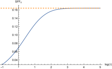
(a) $\text{SFF}_{0}$

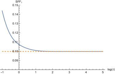
(b) $\text{SFF}_{1}$

Figure 1: Plot of 1(a) $\text{SFF}_{0}$ and 1(b) $\text{SFF}_{1}$ for JT gravity. The horizontal axis is $\log\tau$. We set $\beta=1$ in this figure. $\text{SFF}_{g}$ approaches $\langle Z(2\beta)\rangle_{g}$ as $\tau\to\infty$ (shown by orange dashed lines).

5 Computation of SFF

In this section we formulate a systematic method of computing the small $\hbar$ expansion of the $\tau$-scaling limit of the SFF in the general background $\{t_{k}\}$ of topological gravity. In section 5.1 we will first derive a key relation

$$\partial_{\tau}\partial_{0}\text{SFF} =\frac{\mathrm{i}}{\hbar}\left[W_{1}\left(\beta+\frac{\mathrm{i}\tau}{\hbar}\right)\partial_{0}W_{1}\left(\beta-\frac{\mathrm{i}\tau}{\hbar}\right)-\partial_{0}W_{1}\left(\beta+\frac{\mathrm{i}\tau}{\hbar}\right)W_{1}\left(\beta-\frac{\mathrm{i}\tau}{\hbar}\right)\right],$$ (66)

which relates SFF with (the $t_{0}$-derivative of) the one-point function

$$W_{1}\left(\beta\pm\frac{\mathrm{i}\tau}{\hbar}\right)=\hbar\partial_{0}\left\langle Z\left(\beta\pm\frac{\mathrm{i}\tau}{\hbar}\right)\right\rangle.$$ (67)

Here $\partial_{k}:=\partial_{t_{k}}$. The relation (66) enables us to compute the small $\hbar$ expansion of the SFF from that of the one-point function $W_{1}(\beta\pm\tfrac{\mathrm{i}\tau}{\hbar})$. As we will describe in section 5.2, the small $\hbar$ expansion of $W_{1}(\beta\pm\tfrac{\mathrm{i}\tau}{\hbar})$ can be obtained by the method developed in Okuyama:2021cub with a slight modification. This is based on the KdV equation. We will then explain in section 5.3 how to integrate $\partial_{\tau}\partial_{0}\text{SFF}$ to obtain the small $\hbar$ expansion of the SFF.

5.1 Derivation of the key differential equation

In this subsection we will derive (66). As we have already seen in the previous sections, the one- and two-point functions can be expressed in terms of the CD kernel as Okuyama:2020ncd

$$\begin{aligned} \langle Z(\beta)\rangle&=\int dEe^{-\beta E}K(E,E),\\ \langle Z(\beta_{1})Z(\beta_{2})\rangle_{\rm c}&=\langle Z(\beta_{1}+\beta_{2})\rangle-\int dE_{1}dE_{2}e^{-\beta_{1}E_{1}-\beta_{2}E_{2}}K(E_{1},E_{2})^{2}.\end{aligned}$$ (68)

The CD kernel is written as

$$K(E_{1},E_{2})=\frac{\hbar\partial_{0}\psi(E_{1})\psi(E_{2})-\hbar\partial_{0}\psi(E_{2})\psi(E_{1})}{-E_{1}+E_{2}},$$ (69)

where $\psi(E)$ is the Baker-Akhiezer function. It satisfies the Schrödinger equation

$$-(\hbar^{2}\partial_{0}^{2}+u)\psi(E)=E\psi(E).$$ (70)

By using this equation it immediately follows from (69) that

$$\hbar\partial_{0}K(E_{1},E_{2})=\psi(E_{1})\psi(E_{2}).$$ (71)

Then we have

$$\hbar\partial_{0}\langle Z(\beta)\rangle =W_{1}(\beta)=\int dEe^{-\beta E}\psi(E)^{2},$$ (72)

$$\hbar\partial_{0}\langle Z(\beta_{1})Z(\beta_{2})\rangle_{\rm c} =W_{1}(\beta_{1}+\beta_{2})-\int dE_{1}dE_{2}e^{-\beta_{1}E_{1}-\beta_{2}E_{2}}2\psi(E_{1})\psi(E_{2})K(E_{1},E_{2}).$$

When $\beta_{1,2}=\beta\pm\mathrm{i}\tau\hbar^{-1}$, we find

$$\partial_{\tau}\partial_{0}\langle Z(\beta_{1})Z(\beta_{2})\rangle_{\rm c}$$ (73)

$$=-\frac{\mathrm{i}}{\hbar^{2}}\int dE_{1}dE_{2}e^{-\beta_{1}E_{1}-\beta_{2}E_{2}}2\psi(E_{1})\psi(E_{2})(-E_{1}+E_{2})K(E_{1},E_{2})$$

$$=-\frac{\mathrm{i}}{\hbar^{2}}\int dE_{1}dE_{2}e^{-\beta_{1}E_{1}-\beta_{2}E_{2}}2\psi(E_{1})\psi(E_{2})\left[\hbar\partial_{0}\psi(E_{1})\psi(E_{2})-\hbar\partial_{0}\psi(E_{2})\psi(E_{1})\right]$$

$$=-\frac{\mathrm{i}}{\hbar}\int dE_{1}dE_{2}e^{-\beta_{1}E_{1}-\beta_{2}E_{2}}\left[\partial_{0}\psi(E_{1})^{2}\psi(E_{2})^{2}-\psi(E_{1})^{2}\partial_{0}\psi(E_{2})^{2}\right]$$

$$=-\frac{\mathrm{i}}{\hbar}\left[\partial_{0}W_{1}(\beta_{1})W_{1}(\beta_{2})-W_{1}(\beta_{1})\partial_{0}W_{1}(\beta_{2})\right].$$

Thus we have derived (66).

5.2 Small $\hbar$ expansion of one-point function

Let us next consider the small $\hbar$ expansion of $W_{1}\left(\beta\pm\frac{\mathrm{i}\tau}{\hbar}\right)$. We can restrict ourselves to the case of $W_{1}\left(\beta+\frac{\mathrm{i}\tau}{\hbar}\right)$ without loss of generality, as $W_{1}\left(\beta-\frac{\mathrm{i}\tau}{\hbar}\right)$ is immediately obtained by complex conjugation. The expansion can be done in two ways. One way, which is easier to understand, is to use the results of the ’t Hooft expansion computed in Okuyama:2021cub :

$$W_{1}\left(\beta\right)=\exp\left[\sum_{n=0}^{\infty}\hbar^{n-1}\widetilde{G}_{n}(\lambda)\right],\quad\lambda=\hbar\beta\ \mbox{fixed.}$$ (74)

Given this expansion, the small $\hbar$ expansion of $W_{1}\left(\beta+\frac{\mathrm{i}\tau}{\hbar}\right)$ is obtained by merely substituting $\lambda=\mathrm{i}\tau+\beta\hbar$ into the expansion and then re-expanding it in $\hbar$ as

$$\begin{aligned} W_{1}\left(\beta+\frac{\mathrm{i}\tau}{\hbar}\right)&=\exp\biggl{[}\hbar^{-1}\widetilde{G}_{0}(\mathrm{i}\tau)+\left(\widetilde{G}_{1}(\mathrm{i}\tau)+\widetilde{G}_{0}^{\prime}(\mathrm{i}\tau)\beta\right)\\ &\hskip 40.00006pt+\hbar\left(\widetilde{G}_{2}(\mathrm{i}\tau)+\widetilde{G}_{1}^{\prime}(\mathrm{i}\tau)\beta+\frac{1}{2}\widetilde{G}_{0}^{\prime\prime}(\mathrm{i}\tau)\beta^{2}\right)+{\cal O}(\hbar^{2})\biggr{]}.\end{aligned}$$ (75)

More specifically, the first few $\widetilde{G}_{n}$ are given by Okuyama:2021cub

$$\begin{aligned} \widetilde{G}_{0}&=-E_{0}\lambda+\sum_{\begin{subarray}{c}j_{a}\geq 0\\[1.50694pt] \sum_{a}j_{a}=k\\[1.50694pt] \sum_{a}aj_{a}=n\end{subarray}}\frac{(2n+k+1)!}{(2n+3)!}\frac{\lambda^{2n+3}}{2^{n+1}s^{2n+k+2}}\prod_{a=1}^{\infty}\frac{I_{a+1}^{j_{a}}}{j_{a}!(2a+1)!!^{j_{a}}}\\ &=-E_{0}\lambda+\frac{1}{12s^{2}}\lambda^{3}+\frac{I_{2}}{60s^{5}}\lambda^{5}+\left(\frac{I_{2}^{2}}{144s^{8}}+\frac{I_{3}}{840s^{7}}\right)\lambda^{7}+{\cal O}(\lambda^{9}),\\[4.30554pt] \widetilde{G}_{1}&=\frac{1}{2}\log\left[\frac{\hbar}{8\pi}\frac{\partial_{\lambda}E(\lambda)}{E(\lambda)-E_{0}}\right],\\ \widetilde{G}_{2}&=\frac{\mathrm{i}I_{2}}{12s^{2}z(\lambda)}-\frac{5\mathrm{i}}{24sz(\lambda)^{3}}-\frac{3E^{(1)}}{8z(\lambda)^{4}}+\frac{E^{(2)}}{4z(\lambda)^{2}E^{(1)}}-\frac{E^{(3)}}{8\left(E^{(1)}\right)^{2}}+\frac{\left(E^{(2)}\right)^{2}}{6\left(E^{(1)}\right)^{3}},\end{aligned}$$ (76)

where

$$E(\lambda)=-\partial_{\lambda}\widetilde{G}_{0},\qquad z(\lambda)=\sqrt{E(\lambda)-E_{0}},\qquad E^{(j)}=\partial_{\lambda}^{j}E(\lambda).$$ (77)

$I_{k}$ and $s=1-I_{1}$ were defined in section 2. From this one obtains

$$W_{1}\left(\beta+\frac{\mathrm{i}\tau}{\hbar}\right)=e^{G\left(\beta+\frac{\mathrm{i}\tau}{\hbar}\right)}=\exp\left[\sum_{n=0}^{\infty}\hbar^{n-1}G_{n}(\beta,\tau,\{I_{k}\})\right]$$ (78)

with

$$\begin{aligned} G_{0}&=\widetilde{G}_{0}(\mathrm{i}\tau),\\ G_{1}&=\frac{1}{2}\log\left[\frac{\hbar}{8\pi\mathrm{i}}\frac{\partial_{\tau}E_{\tau}}{E_{\tau}-E_{0}}\right]-\beta E_{\tau},\\ G_{2}&=\mathrm{i}\left[\frac{I_{2}}{12s^{2}z_{\tau}}-\frac{5}{24sz_{\tau}^{3}}+\frac{3e(1)}{8z_{\tau}^{4}}-\frac{e(2)}{4z_{\tau}^{2}e(1)}+\frac{e(3)}{8e(1)^{2}}-\frac{e(2)^{2}}{6e(1)^{3}}\right.\\ &\hskip 20.00003pt\left.+\left(\frac{e(1)}{2z_{\tau}^{2}}-\frac{e(2)}{2e(1)}\right)\beta+\frac{e(1)}{2}\beta^{2}\right].\end{aligned}$$ (79)

Here $E_{\tau}=E(\mathrm{i}\tau)$, $z_{\tau}=\sqrt{E_{\tau}-E_{0}}=z(\mathrm{i}\tau)$ and $e(j)=\partial_{\tau}^{j}E_{\tau}=\mathrm{i}^{j}E^{(j)}(\mathrm{i}\tau)$.

The other way to compute the small $\hbar$ expansion of $W_{1}\left(\beta+\frac{\mathrm{i}\tau}{\hbar}\right)$, which is technically more efficient, is to solve the KdV equation directly with the expansion (78). This can be done by the method of Okuyama:2021cub with only a slight modification. In what follows let us describe the method in our present notation. First, recall that $W_{1}=W_{1}\left(\beta+\frac{\mathrm{i}\tau}{\hbar}\right)$ satisfies the KdV equation Okuyama:2019xbv

$$\partial_{1}W_{1}=u\partial_{0}W_{1}+\frac{\hbar^{2}}{6}\partial_{0}^{3}W_{1}.$$ (80)

In terms of $G=\log W_{1}$, this is written as

$$\partial_{1}G=u\partial_{0}G+\frac{\hbar^{2}}{6}\Bigl{(}\partial_{0}^{3}G+3\partial_{0}G\partial_{0}^{2}G+(\partial_{0}G)^{3}\Bigr{)}.$$ (81)

Here, $u$ is the specific heat of the general topological gravity. It obeys the KdV equation and its genus expansion

$$u=\sum_{g=0}^{\infty}2^{g}u_{g}\hbar^{2g}$$ (82)

was computed by means of a recurrence relation. Note, in particular, that the leading order part is equal to the threshold energy

$$u_{0}=-E_{0}.$$ (83)

By plugging the expansions (82) and

$$G=\sum_{n=0}^{\infty}\hbar^{n-1}G_{n}$$ (84)

into (81), one obtains the recurrence relation

$$-\partial_{s}G_{0} =\frac{1}{6}(\partial_{0}G_{0})^{3},$$ (85)

$$DG_{1} =\frac{1}{2}\partial_{0}G_{0}\partial_{0}^{2}G_{0}$$ (86)

for $n=0,1$ and

$$\begin{aligned} DG_{n}=\frac{1}{6}\sum_{\begin{subarray}{c}0\leq i,j,k<n\\[3.01389pt] i+j+k=n\end{subarray}}\partial_{0}G_{i}\partial_{0}G_{j}\partial_{0}G_{k}+\frac{1}{2}\sum_{k=0}^{n-1}\partial_{0}G_{n-k-1}\partial_{0}^{2}G_{k}+\frac{1}{6}\partial_{0}^{3}G_{n-2}+\sum_{k=1}^{\lfloor\frac{n}{2}\rfloor}2^{k}u_{k}\partial_{0}G_{n-2k}\end{aligned}$$ (87)

for $n\geq 2$. Here we have introduced the differential operator

$$D:=-\partial_{s}-\frac{1}{2}(\partial_{0}G_{0})^{2}\partial_{0}.$$ (88)

Note also that instead of $t_{0},t_{1}$ we regard $s$ and $E_{0}$ as independent variables and treat $t_{k\geq 2}$ as parameters Okuyama:2019xbv . From this viewpoint $\partial_{0,1}$ are understood as

$$\partial_{0}=-\frac{1}{s}\left(\partial_{E_{0}}+I_{2}\partial_{s}\right),\qquad\partial_{1}=-E_{0}\partial_{0}-\partial_{s}.$$ (89)

To solve the recurrence relation (85)–(87), it is helpful to recall some relevant formulas (see Okuyama:2021cub ):

$$\begin{aligned} \partial_{0}s&=-\frac{I_{2}}{s},\quad&\partial_{0}I_{n}&=\frac{I_{n+1}}{s}\quad(n\geq 1),\ \\ \partial_{0}G_{0}&=2\mathrm{i}z_{\tau},&\partial_{0}z_{\tau}&=\frac{1}{2sz_{\tau}}-\frac{\partial_{\tau}z_{\tau}}{z_{\tau}},&\partial_{0}e(j)&=-2\partial_{\tau}^{j+1}z_{\tau},\\ \partial_{s}z_{\tau}&=-e(1).\end{aligned}$$ (90)

The differential operator (88) is then written as

$$D=-\partial_{s}+2z_{\tau}^{2}\partial_{0}.$$ (91)

It has the properties

$$Dz_{\tau} =\frac{z_{\tau}}{s},\qquad DE_{\tau}=0,$$ (92)

$$De(n) =8\sum_{k=0}^{n-1}\sum_{\ell=0}^{k}\sum_{m=0}^{\ell}\frac{k!}{(k-\ell)!(\ell-m)!m!}\partial_{\tau}^{(n-\ell)}z_{\tau}\,\partial_{\tau}^{(\ell-m)}z_{\tau}\,\partial_{\tau}^{(m+1)}z_{\tau}.$$ (93)

As explained in Okuyama:2020vrh , $\partial_{\tau}^{n}z_{\tau}$ can be expressed in terms of $e(j)$ and $z_{\tau}$:

$$\begin{aligned} \partial_{\tau}z_{\tau}&=\frac{e(1)}{2z_{\tau}},\\ \partial_{\tau}^{2}z_{\tau}&=\frac{e(2)}{2z_{\tau}}-\frac{e(1)^{2}}{4z_{\tau}^{3}},\\ \partial_{\tau}^{3}z_{\tau}&=\frac{e(3)}{2z_{\tau}}-\frac{3e(1)e(2)}{4z_{\tau}^{3}}+\frac{3e(1)^{3}}{8z_{\tau}^{5}}.\end{aligned}$$ (94)

We are now in a position to solve the recurrence relation. In Okuyama:2021cub the recurrence relation (85)–(87) was solved with the initial data

$$\begin{aligned} G_{0}^{\text{before}}=\widetilde{G}_{0}(\mathrm{i}\tau),\qquad G_{1}^{\text{before}}=\frac{1}{2}\log\left[\frac{\hbar}{8\pi\mathrm{i}}\frac{\partial_{\tau}E_{\tau}}{E_{\tau}-E_{0}}\right].\end{aligned}$$ (95)

Here, we would like to solve the same recurrence relation with the initial data given in (79). The only difference from Okuyama:2021cub is that here $G_{1}$ has an extra $\beta$-dependent term $-\beta E_{\tau}$. It is clear from (92) that (86) is satisfied by $G_{1}$ with this term, given that (86) is satisfied by $G_{1}^{\text{before}}$.

To solve the recurrence relation, we can use almost the same algorithm we developed in Okuyama:2021cub . The only difference is the step (v), which is modified accordingly so that it works for the $\beta$-dependent parts as well. The modified algorithm is as follows:

1. Compute the r.h.s. of (87) and express it as a polynomial in the variables $s^{-1}$, $I_{k\geq 2}$, $z_{\tau}^{-1}$, $e(1)^{-1}$ and $e(n),\ {n\geq 1}$.

2. Let $s^{-m}f\bigl{(}I_{k},z_{\tau},e(n)\bigr{)}$ denote the highest-order part in $s^{-1}$ of the obtained expression. This part can arise only from

   $$D\left(\frac{f\bigl{(}I_{k},z_{\tau},e(n)\bigr{)}}{2(m-2)s^{m-2}z_{\tau}^{2}I_{2}}\right).$$ (96)

   Therefore subtract this from the obtained expression.

3. Repeat procedure (ii) down to $m=3$. Then all the terms of order $s^{-2}$ automatically disappear and the remaining terms are of order $s^{-1}$ or $s^{0}$. Note also that the expression does not contain any $I_{k}$.

4. In the result of (iii), collect all the terms of order $s^{-1}$ and let $s^{-1}z_{\tau}\partial_{z_{\tau}}g\bigl{(}z_{\tau},e(n)\bigr{)}$ denote the sum of them. This part arises from

   $$Dg\bigl{(}z_{\tau},e(n)\bigr{)}.$$ (97)

   Therefore subtract this from the result of (iii). The remainder turns out to be independent of $s$.

5. In the obtained expression, let

   $$\frac{e(1)^{m}h\bigl{(}e(n\geq 2)\bigr{)}}{z_{\tau}}$$ (98)

   denote the part which is of the order $z_{\tau}^{-1}$ as well as of the highest order in $e(1)$. This part arises from

   $$D\left[-\frac{1}{2e(1)}\int^{\tilde{a}}da\left(a^{-1}e(1)\right)^{m}h\bigl{(}e(n)\to a^{-n-1}e(n)\bigr{)}\right]_{\tilde{a}=1}.$$ (99)

   (Here, $a$ and $\tilde{a}$ are intermediate formal variables.) Therefore subtract this from the obtained expression.

6. Repeat procedure (v) until the resulting expression vanishes.

7. By summing up all the above-obtained primitive functions, we obtain $G_{n}$.

Using the above algorithm we have computed $G_{n}$ for $n\leq 12$. For instance, $G_{3}$ is computed as

$$\begin{aligned} G_{3}&=-\frac{5}{32s^{2}z_{\tau}^{6}}+\frac{I_{2}}{8s^{3}z_{\tau}^{4}}-\frac{I_{3}}{24s^{3}z_{\tau}^{2}}-\frac{I_{2}^{2}}{12s^{4}z_{\tau}^{2}}-\frac{5I_{2}e(1)}{96s^{2}z_{\tau}^{5}}-\frac{3e(1)^{2}}{4z_{\tau}^{8}}+\frac{35e(1)}{64sz_{\tau}^{7}}+\frac{11e(2)}{16z_{\tau}^{6}}\\ &\hskip 10.00002pt-\frac{3e(3)}{16z_{\tau}^{4}e(1)}-\frac{5e(2)}{32sz_{\tau}^{5}e(1)}+\frac{I_{2}e(2)}{48s^{2}z_{\tau}^{3}e(1)}+\frac{e(4)}{16z_{\tau}^{2}e(1)^{2}}+\frac{e(2)^{2}}{8z_{\tau}^{4}e(1)^{2}}-\frac{e(5)}{48e(1)^{3}}\\ &\hskip 10.00002pt-\frac{7e(2)e(3)}{24z_{\tau}^{2}e(1)^{3}}+\frac{e(3)^{2}}{8e(1)^{4}}+\frac{e(2)^{3}}{4z_{\tau}^{2}e(1)^{4}}+\frac{e(2)e(4)}{6e(1)^{4}}-\frac{3e(2)^{2}e(3)}{4e(1)^{5}}+\frac{e(2)^{4}}{2e(1)^{6}}\\ &\hskip 10.00002pt+\left(\frac{5e(1)}{16sz_{\tau}^{5}}-\frac{3e(1)^{2}}{4z_{\tau}^{6}}+\frac{5e(2)}{8z_{\tau}^{4}}-\frac{I_{2}e(1)}{24s^{2}z_{\tau}^{3}}-\frac{e(3)}{4z_{\tau}^{2}e(1)}+\frac{e(4)}{8e(1)^{2}}+\frac{e(2)^{2}}{4z_{\tau}^{2}e(1)^{2}}\right.\\ &\hskip 28.00006pt\left.-\frac{7e(2)e(3)}{12e(1)^{3}}+\frac{e(2)^{3}}{2e(1)^{4}}\right)\beta+\left(-\frac{e(1)^{2}}{4z_{\tau}^{4}}+\frac{e(2)}{4z_{\tau}^{2}}+\frac{e(2)^{2}}{4e(1)^{2}}-\frac{e(3)}{4e(1)}\right)\beta^{2}+\frac{e(2)}{6}\beta^{3}.\end{aligned}$$ (100)

Let us finally comment on the small $\hbar$ expansion of $W_{1}\left(\beta-\frac{\mathrm{i}\tau}{\hbar}\right)$. As we mentioned already, it is obtained from (78) by complex conjugation:

$$W_{1}\left(\beta-\frac{\mathrm{i}\tau}{\hbar}\right)=\exp\left[\sum_{n=0}^{\infty}\hbar^{n-1}\overline{G_{n}}\right].$$ (101)

Furthermore, $\overline{G_{n}}$ is related to $G_{n}$ by

$$\overline{G_{n}}=(-1)^{n+1}G_{n}+\frac{\pi\mathrm{i}}{2}\delta_{n,1}.$$ (102)

This can be shown directly for $n=0,1$ and inductively for $n\geq 2$ by using the recurrence relation (87).

5.3 Small $\hbar$ expansion of SFF

Using the results obtained above, one can compute the small $\hbar$ expansion of the SFF. Substituting (78), (101) and the explicit form of $G_{1}$ in (79) into (66), one obtains

$$\begin{aligned} \partial_{\tau}\partial_{0}\text{SFF}&=\frac{\mathrm{i}}{\hbar}(\partial_{0}\overline{G}-\partial_{0}G)e^{G+\overline{G}}\\ &=-\frac{2\mathrm{i}}{\hbar}\sum_{k=0}^{\infty}\hbar^{2k-1}\partial_{0}G_{2k}\exp\left(G_{1}+\overline{G_{1}}+2\sum_{k=1}^{\infty}\hbar^{2k}G_{2k+1}\right)\\ &=\frac{e^{-2\beta E_{\tau}}}{4\pi\mathrm{i}}\frac{\partial_{\tau}E_{\tau}}{E_{\tau}-E_{0}}\sum_{k=0}^{\infty}\hbar^{2k-1}\partial_{0}G_{2k}\exp\left(\sum_{k=1}^{\infty}2G_{2k+1}\hbar^{2k}\right)\\ &=:\frac{e^{-2\beta E_{\tau}}}{2\pi\hbar}\sum_{n=0}^{\infty}c_{n}\hbar^{2n},\end{aligned}$$ (103)

where the first two of $c_{n}$ are computed as

$$\begin{aligned} c_{0}&=\frac{e(1)}{z_{\tau}},\\ c_{1}&=\frac{e(1)e(2)}{3z_{\tau}}\beta^{3}+\left(-\frac{3e(1)^{3}}{8z_{\tau}^{5}}+\frac{e(1)e(2)}{4z_{\tau}^{3}}-\frac{e(3)}{2z_{\tau}}+\frac{e(2)^{2}}{2z_{\tau}e(1)}\right)\beta^{2}\\ &\hskip 10.00002pt+\left(-\frac{15e(1)^{3}}{16z_{\tau}^{7}}+\frac{3e(1)e(2)}{4z_{\tau}^{5}}-\frac{e(3)}{4z_{\tau}^{3}}+\frac{3e(1)^{2}}{8sz_{\tau}^{6}}-\frac{I_{2}e(1)^{2}}{12s^{2}z_{\tau}^{4}}\right.\\ &\hskip 28.00006pt\left.+\frac{e(4)}{4z_{\tau}e(1)}+\frac{e(2)^{2}}{4z_{\tau}^{3}e(1)}-\frac{7e(2)e(3)}{6z_{\tau}e(1)^{2}}+\frac{e(2)^{3}}{z_{\tau}e(1)^{3}}\right)\beta\\ &\hskip 10.00002pt-\frac{5e(1)}{32s^{2}z_{\tau}^{7}}+\frac{25e(1)e(2)}{32z_{\tau}^{7}}-\frac{3e(3)}{16z_{\tau}^{5}}+\frac{9e(1)^{2}}{16sz_{\tau}^{8}}+\frac{I_{2}e(1)}{8s^{3}z_{\tau}^{5}}-\frac{I_{2}^{2}e(1)}{12s^{4}z_{\tau}^{3}}-\frac{I_{2}e(1)^{2}}{12s^{2}z_{\tau}^{6}}-\frac{3e(2)}{16sz_{\tau}^{6}}\\ &\hskip 10.00002pt-\frac{I_{3}e(1)}{24s^{3}z_{\tau}^{3}}+\frac{I_{2}e(2)}{24s^{2}z_{\tau}^{4}}-\frac{105e(1)^{3}}{128z_{\tau}^{9}}+\frac{3e(2)^{2}}{32z_{\tau}^{5}e(1)}+\frac{e(4)}{16z_{\tau}^{3}e(1)}-\frac{e(5)}{24z_{\tau}e(1)^{2}}-\frac{7e(2)e(3)}{24z_{\tau}^{3}e(1)^{2}}\\ &\hskip 10.00002pt+\frac{e(2)^{3}}{4z_{\tau}^{3}e(1)^{3}}+\frac{e(3)^{2}}{4z_{\tau}e(1)^{3}}+\frac{e(2)e(4)}{3z_{\tau}e(1)^{3}}-\frac{3e(2)^{2}e(3)}{2z_{\tau}e(1)^{4}}+\frac{e(2)^{4}}{z_{\tau}e(1)^{5}}.\end{aligned}$$ (104)

Let us next consider the expansion

$$\partial_{\tau}\text{SFF}=\frac{e^{-2\beta E_{\tau}}}{2\pi\hbar}\sum_{n=0}^{\infty}b_{n}\hbar^{2n}.$$ (105)

Comparing (105) with (103), we see that $b_{n}$ and $c_{n}$ are related as

$$\begin{aligned} c_{n}&=e^{2\beta E_{\tau}}\partial_{0}e^{-2\beta E_{\tau}}b_{n}\\ &=\left(\partial_{0}-2\beta\partial_{0}E_{\tau}\right)b_{n}\\ &=\left(\partial_{0}+2\beta\frac{e(1)}{z_{\tau}}\right)b_{n}.\end{aligned}$$ (106)

For $n=0$, we immediately see that $b_{0}=1/(2\beta)$ gives $c_{0}$ in (104). For $n\geq 1$, let us assume that $b_{n}$ is a polynomial in $\beta$. Then, the highest-order term of this polynomial is determined as that of $c_{n}$ divided by $2\beta e(1)/z_{\tau}$. Subtracting this contribution from both sides of (106), one can determine the next to the highest-order term in the same manner. In this way, one can determine $b_{n}$ as a polynomial of $\beta$ without integrating in $t_{0}$. For instance, the first two of them are

$$\begin{aligned} b_{0}&=\frac{1}{2\beta},\\ b_{1}&=\frac{e(2)}{6}\beta^{2}+\left(-\frac{e(1)^{2}}{8z_{\tau}^{4}}-\frac{e(3)}{6e(1)}+\frac{e(2)^{2}}{4e(1)^{2}}\right)\beta\\ &\hskip 10.00002pt-\frac{I_{2}e(1)}{24s^{2}z_{\tau}^{3}}+\frac{e(2)}{16z_{\tau}^{4}}+\frac{e(1)}{16sz_{\tau}^{5}}-\frac{e(1)^{2}}{8z_{\tau}^{6}}+\frac{e(4)}{24e(1)^{2}}-\frac{e(2)e(3)}{4e(1)^{3}}+\frac{e(2)^{3}}{4e(1)^{4}}.\end{aligned}$$ (107)

Let us finally consider the small $\hbar$ expansion (3) of the SFF:

$$\begin{aligned} \text{SFF}&=\text{SFF}_{g=0}+\text{SFF}_{g\geq 1}\\ &=\hbar^{-1}\text{SFF}_{0}+\sum_{g=1}^{\infty}\hbar^{2g-1}\text{SFF}_{g}.\end{aligned}$$ (108)

The leading term $\text{SFF}_{0}$ is given in (22). It is easy to verify that the $\tau$-derivative of (22) reproduces the leading order part of (105) with $b_{0}=1/(2\beta)$. Here, we are interested in the higher order part $\text{SFF}_{g\geq 1}$. As explained in section 3 (see, in particular (28)), a key feature of $\text{SFF}_{g\geq 1}$ is that it takes the form

$$\begin{aligned} \mathrm{SFF}_{g\geq 1}&=\operatorname{Erf}\left(\sqrt{2\beta}z_{\tau}\right)\langle Z(2\beta)\rangle_{g\geq 1}+\frac{e^{-2\beta E_{\tau}}}{2\pi\hbar}\sum_{g=1}^{\infty}a_{g}\hbar^{2g}\end{aligned}$$ (109)

with $a_{g}$ being polynomial in $\beta$. The small $\hbar$ expansion of the one-point function $\langle Z(2\beta)\rangle$ was computed in Okuyama:2019xbv :

$$\langle Z(2\beta)\rangle_{g\geq 1}=\frac{e^{-2\beta E_{0}}}{\sqrt{2\pi(2\beta)^{3}}\sqrt{2}\hbar}\sum_{g=1}^{\infty}\hbar^{2g}2^{g}Z_{g}(2\beta),$$ (110)

where

$$\begin{aligned} Z_{1}(\beta)&=\frac{1}{24s}\beta^{3}+\frac{I_{2}}{24s^{2}}\beta^{2},\\ Z_{2}(\beta)&=\frac{1}{1152s^{3}}\beta^{6}+\frac{29I_{2}}{5760s^{4}}\beta^{5}+\left(\frac{7I_{2}^{2}}{480s^{5}}+\frac{29I_{3}}{5760s^{4}}\right)\beta^{4}+\left(\frac{7I_{2}^{3}}{288s^{6}}+\frac{29I_{2}I_{3}}{1440s^{5}}+\frac{I_{4}}{384s^{4}}\right)\beta^{3}\\ &\hskip 10.00002pt+\left(\frac{7I_{2}^{4}}{288s^{7}}+\frac{5I_{2}^{2}I_{3}}{144s^{6}}+\frac{29I_{3}^{2}}{5760s^{5}}+\frac{11I_{2}I_{4}}{1440s^{5}}+\frac{I_{5}}{1152s^{4}}\right)\beta^{2}.\end{aligned}$$ (111)

Comparing (109) with (105), we see that $a_{g}$ and $b_{g}$ are related as

$$b_{g}=\frac{e(1)}{2\beta z_{\tau}}2^{g}Z_{g}(2\beta)+\bigl{(}\partial_{\tau}-2\beta e(1)\bigr{)}a_{g}.$$ (112)

Given that $a_{g}$ are polynomials in $\beta$, we can calculate them from $b_{g}$ without integrating in $\tau$, in essentially the same way as we obtained $b_{g}$ from $c_{g}$. For instance, $a_{1}$ is obtained as

$$a_{1} =\left(\frac{1}{6sz_{\tau}}-\frac{e(2)}{12e(1)}\right)\beta+\frac{e(1)}{16z_{\tau}^{4}}+\frac{I_{2}}{12s^{2}z_{\tau}}-\frac{1}{24sz_{\tau}^{3}}+\frac{e(3)}{24e(1)^{2}}-\frac{e(2)^{2}}{12e(1)^{3}}.$$ (113)

One sees that the terms which do not contain $e(j)$ precisely give $d_{1}$ in (30); the other terms comprise $f_{1}$ given by (31) with (33). The expression of $a_{2}$ is already rather long and we relegate it to Appendix B. We have computed $a_{g}$ for $g\leq 5$.

6 Higher order corrections to CD kernel

In this section we consider the higher order correction of the CD kernel beyond the sine kernel approximation. That is, we consider a small $\hbar$ expansion of the CD kernel. In principle, this is not a difficult task since the CD kernel is expressed as a bilinear form (69) in terms of the BA function $\psi(E)$ whose $\hbar$-expansion was calculated Okuyama:2020ncd . The purpose of this section is to present a concrete, technically efficient method.

6.1 Small $\hbar$ expansion of BA function

To compute the expansion of the CD kernel, one first needs to compute the small $\hbar$ expansion of $\psi(E+\frac{1}{2}\hbar\omega)$ rather than $\psi(E)$. Of course, this is obtained by re-expanding the results of Okuyama:2020ncd with the replacement $E\to E+\frac{1}{2}\hbar\omega$. For the sake of technical efficiency, however, here we compute the expansion

$$\log\psi(E+\tfrac{1}{2}\hbar\omega)=A(E+\tfrac{1}{2}\hbar\omega)=\sum_{n=0}^{\infty}\hbar^{n-1}A_{n}(E,\omega)$$ (114)

directly by means of a recurrence relation.

It was derived in Okuyama:2020ncd that

$$v(E):=\hbar\partial_{0}A(E)$$ (115)

satisfies the equation

$$\begin{aligned} v^{2}+\hbar\partial_{0}v&=-E-u.\end{aligned}$$ (116)

Here, $u$ is the specific heat of the general topological gravity and we again assume that its genus expansion (82) is given. Since we want to compute the $\hbar$ expansion of $\psi$ with a shifted argument, we replace $E$ in (116) by $E+\tfrac{1}{2}\hbar\omega$ and plug the expansion of the form

$$v=v(E+\tfrac{1}{2}\hbar\omega)=\sum_{n=0}^{\infty}\hbar^{n}v_{n}(E,\omega)$$ (117)

into (116). Expanding both sides of the equation in $\hbar$, we obtain the recurrence relation

$$\begin{aligned} v_{0}^{2}&=-E+E_{0},\qquad 2v_{0}v_{1}+\partial_{0}v_{0}=-\frac{\omega}{2},\\ v_{n}&=-\frac{1}{2v_{0}}\left(\partial_{0}v_{n-1}+\sum_{k=1}^{n-1}v_{k}v_{n-k}+\left\{\begin{array}[]{ll}2^{\frac{n}{2}}u_{\frac{n}{2}}&\mbox{($n$ even)}\\ 0&\mbox{($n$ odd)}\end{array}\right.\right),\quad n\geq 2.\end{aligned}$$ (118)

The first two equations are solved as

$$\begin{aligned} v_{0}&=\mathrm{i}z=\mathrm{i}\sqrt{E-E_{0}},\\ v_{1}&=-\frac{1}{4sz^{2}}+\frac{\mathrm{i}\omega}{4z}.\end{aligned}$$ (119)

$v_{n}\ (n\geq 2)$ are also immediately obtained by the recurrence relation given the form of $u_{g}$. For instance, using

$$u_{1}=\frac{I_{2}^{2}}{12s^{4}}+\frac{I_{3}}{24s^{3}}$$ (120)

one obtains

$$\begin{aligned} v_{2}&=\mathrm{i}\left(\frac{I_{2}^{2}}{12zs^{4}}+\frac{I_{3}}{24zs^{3}}-\frac{I_{2}}{8z^{3}s^{3}}+\frac{5}{32z^{5}s^{2}}\right)+\frac{1}{8z^{4}s}\omega-\mathrm{i}\frac{1}{32z^{3}}\omega^{2},\\ v_{3}&=-\frac{I_{2}^{3}}{6s^{6}z^{2}}-\frac{7I_{2}I_{3}}{48s^{5}z^{2}}+\frac{11I_{2}^{2}}{48s^{5}z^{4}}-\frac{I_{4}}{48s^{4}z^{2}}+\frac{I_{3}}{12s^{4}z^{4}}-\frac{9I_{2}}{32s^{4}z^{6}}+\frac{15}{64s^{3}z^{8}}\\ &\hskip 10.00002pt+\mathrm{i}\left(-\frac{I_{2}^{2}}{48s^{4}z^{3}}-\frac{I_{3}}{96s^{3}z^{3}}+\frac{3I_{2}}{32s^{3}z^{5}}-\frac{25}{128s^{2}z^{7}}\right)\omega-\frac{1}{16sz^{6}}\omega^{2}+\mathrm{i}\frac{1}{128z^{5}}\omega^{3}.\end{aligned}$$ (121)

Note that the form of the recurrence relation (118) for $v_{n\geq 2}$ is not affected by the shift $E\to E+\frac{1}{2}\hbar\omega$. The $\omega$-dependence enters entirely through the initial data, i.e. the form of $v_{1}$.

One can easily obtain $A_{n}$ from $v_{n}$ through the relation $\partial_{0}A_{n}=v_{n}$. Due to the structure (89) of $\partial_{0}$, the form of the $s$-dependent part of $A_{n}$ can be determined without integrating in $t_{0}$. (We use a similar logic as we obtained $b_{n}$ from $c_{n}$ in the last section.) The $s$-independent part can also be determined with the help of the formulas (the proofs of which are straightforward)

$$\begin{aligned} \int^{t_{0}}dt_{0}\frac{1}{sz^{2}}&=2\log z,\\ \int^{t_{0}}dt_{0}\frac{1}{sz^{2k}}&=-\frac{1}{(k-1)z^{2(k-1)}}\quad(k\geq 2),\\ \int^{t_{0}}dt_{0}\frac{1}{z^{2k-1}}&=\frac{\Gamma(\frac{3}{2}-k)}{\Gamma(\frac{1}{2})}\rho_{0}^{(k-1)}=\frac{(-2)^{k-1}}{(2k-3)!!}\rho_{0}^{(k-1)}\quad(k\geq 0).\end{aligned}$$ (122)

Here

$$\rho_{0}^{(n)}=\partial_{E}^{n}\rho_{0}(E)\quad(n\geq 0),\qquad\rho_{0}^{(-1)}=\int_{E_{0}}^{E}dE\rho_{0}(E).$$ (123)

We thus obtain

$$\begin{aligned} A_{0}&=\frac{\mathrm{i}}{2}\rho_{0}^{(-1)}=\frac{\mathrm{i}}{2}\int_{E_{0}}^{E}dE\rho_{0}(E),\\ A_{1}&=-\frac{1}{2}\log z+\mathrm{i}\frac{\rho_{0}}{4}\omega-\frac{1}{2}\log(4\pi),\\ A_{2}&=\mathrm{i}\left(\frac{I_{2}}{24s^{2}z}-\frac{5}{48sz^{3}}\right)-\frac{1}{8z^{2}}\omega+\mathrm{i}\frac{\rho_{0}^{(1)}}{16}\omega^{2},\\ A_{3}&=-\frac{I_{2}^{2}}{24s^{4}z^{2}}-\frac{I_{3}}{48s^{3}z^{2}}+\frac{I_{2}}{16s^{3}z^{4}}-\frac{5}{64s^{2}z^{6}}+\mathrm{i}\left(-\frac{I_{2}}{96s^{2}z^{3}}+\frac{5}{64sz^{5}}\right)\omega\\ &\hskip 10.00002pt+\frac{1}{32z^{4}}\omega^{2}+\mathrm{i}\frac{\rho_{0}^{(2)}}{96}\omega^{3}.\end{aligned}$$ (124)

The constant part of $A_{1}$ is determined in accordance with the $\omega=0$ case Okuyama:2020ncd .

6.2 Small $\hbar$ expansion of CD kernel

Let us now compute the small $\hbar$ expansion of the CD kernel. We should first note that this is a WKB-type asymptotic expansion. As is known Saad:2019lba , there appear some qualitative differences between the cases of $E>E_{0}$ and $E<E_{0}$. In this paper we consider the case of $E>E_{0}$. In this case the two independent BA functions are given by

$$\psi(E)\quad\mbox{and}\quad\overline{\psi(E)}=\psi(E)\Big{|}_{z\to-z},$$ (125)

i.e. they are complex conjugate to each other. Due to this complex structure, for $E>E_{0}$ there are two saddles which equally contribute to the CD kernel Saad:2019lba . Therefore, as long as the perturbative expansion in $\hbar$ concerns, the CD kernel is approximated by

$$K(E_{1},E_{2})=\widetilde{K}(E_{1},E_{2})+\widetilde{K}(E_{2},E_{1})$$ (126)

with

$$\begin{aligned} \widetilde{K}(E_{1},E_{2})&=\frac{\hbar\partial_{0}\psi(E_{1})\overline{\psi(E_{2})}-\psi(E_{1})\hbar\partial_{0}\overline{\psi(E_{2})}}{-E_{1}+E_{2}}\\[4.30554pt] &=-\frac{v(E_{1})-\overline{v(E_{2})}}{\hbar\omega}e^{A(E_{1})+\overline{A(E_{2})}}.\end{aligned}$$ (127)

By using the recurrence relation (118) it is easy to prove that

$$\overline{v_{n}(E,-\omega)}=(-1)^{n+1}v_{n}(E,\omega),\qquad\overline{A_{n}(E,-\omega)}=(-1)^{n+1}A_{n}(E,\omega).$$ (128)

Therefore (127) is written as

$$\widetilde{K}(E_{1},E_{2})=-\frac{1}{\hbar\omega}\left(\sum_{k=0}^{\infty}2v_{2k}(E,\omega)\hbar^{2k}\right)\exp\left(\sum_{k=0}^{\infty}2A_{2k+1}(E,\omega)\hbar^{2k}\right).$$ (129)

Similarly, we have

$$\widetilde{K}(E_{2},E_{1})=-\frac{1}{\hbar\omega}\sum_{k=0}^{\infty}2\overline{v_{2k}(E,\omega)}\hbar^{2k}\exp\left[\sum_{k=0}^{\infty}2\overline{A_{2k+1}(E,\omega)}\hbar^{2k}\right].$$ (130)

Thus, the CD kernel is given by

$$K(E_{1},E_{2})=\mathrm{Re}\left\{2\widetilde{K}(E_{1},E_{2})\right\}.$$ (131)

Substituting the explicit form of $A_{1}(E,\omega)$ in (124) we obtain

$$\begin{aligned} 2\pi K(E_{1},E_{2})&=\mathrm{Re}\left\{-\frac{2}{\hbar\omega z}\left(\sum_{k=0}^{\infty}v_{2k}(E,\omega)\hbar^{2k}\right)\exp\left(2\sum_{k=1}^{\infty}A_{2k+1}(E,\omega)\hbar^{2k}\right)e^{\mathrm{i}\omega\rho_{0}/2}\right\}\\ &=\mathrm{Re}\left\{Xe^{\mathrm{i}\omega\rho_{0}/2}\right\}\\ &=\mathrm{Re}\{X\}\cos\frac{\omega\rho_{0}}{2}-\mathrm{Im}\{X\}\sin\frac{\omega\rho_{0}}{2},\end{aligned}$$ (132)

where

$$X:=-\frac{2}{\hbar\omega z}\left(\sum_{k=0}^{\infty}v_{2k}(E,\omega)\hbar^{2k}\right)\exp\left(2\sum_{k=1}^{\infty}A_{2k+1}(E,\omega)\hbar^{2k}\right).$$ (133)

With the forms of $v_{n}$ and $A_{n}$ obtained in (119), (121) and (124), this gives the small $\hbar$ expansion of the CD kernel.

A few comments are in order. First, substituting $v_{0}=\mathrm{i}z$ one sees that the expression (132) correctly reproduces the sine kernel (13) at the order of $\hbar^{-1}$. Second, recall that the diagonal part of the CD kernel, i.e. (132) in the limit of $\omega\to 0$, is equal to the eigenvalue density (44). This is evident for the genus zero part at the order of $\hbar^{-1}$, but also implies that

$$\sum_{g=1}^{\infty}\hbar^{2g-1}\rho_{g}(E)=\mathrm{Re}\{X\}\Big{|}_{\omega=0}.$$ (134)

We checked that this indeed reproduces $\rho_{g}$ in (25) which were obtained from the result of $\langle Z(\beta)\rangle_{g}$ in Okuyama:2019xbv .

By taking (134) into account, the expansion (132) is written explicitly as

$$\begin{aligned} &2\pi K(E_{1},E_{2})\\ &=\frac{2}{\hbar\omega}\Biggl{\{}1+\frac{\omega^{2}}{32z^{4}}\hbar^{2}+\Biggl{[}+\left(-\frac{49I_{2}^{2}}{4608s^{4}z^{6}}-\frac{I_{3}}{192s^{3}z^{6}}+\frac{49I_{2}}{1536s^{3}z^{8}}-\frac{105}{2048s^{2}z^{10}}\right)\omega^{2}\\ &\hskip 40.00006pt+\left(\frac{I_{2}\rho_{0}^{(2)}}{2304s^{2}z^{3}}-\frac{\rho_{0}^{(2)}}{1536sz^{5}}+\frac{11}{2048z^{8}}\right)\omega^{4}-\frac{(\rho_{0}^{(2)})^{2}}{4608}\omega^{6}\Biggr{]}\hbar^{4}+{\cal O}(\hbar^{6})\Biggr{\}}\sin\frac{\omega\rho_{0}}{2}\\ &\hskip 10.00002pt+\Biggl{\{}\left[\rho_{1}+\frac{\rho_{0}^{(2)}}{24}\omega^{2}\right]\hbar\\ &\hskip 18.00005pt+\Biggl{[}\rho_{2}+\left(-\frac{I_{2}}{128s^{2}z^{7}}+\frac{35}{768sz^{9}}\right)\omega^{2}+\left(\frac{\rho_{0}^{(4)}}{1920}+\frac{\rho_{0}^{(2)}}{768z^{4}}\right)\omega^{4}\Biggr{]}\hbar^{3}+{\cal O}(\hbar^{5})\Biggr{\}}\cos\frac{\omega\rho_{0}}{2}.\end{aligned}$$ (135)

Observe that there appear several derivatives of $\rho_{0}$ at higher orders. These derivatives in fact have their origin in the integral (43) and are neatly absorbed if one recasts the above result into the form (42).

7 Conclusions and outlook

In this paper we have computed the higher order corrections of the SFF in the $\tau$-scaling limit for an arbitrary background $\{t_{k}\}$ of topological gravity. We have also shown that these corrections of the SFF can be obtained by the Fourier transform of the CD kernel by including the corrections to the sine kernel formula. As we can see from Figure 1, $\text{SFF}_{g\geq 1}$ approaches a constant at late times which gives a correction to the value of the plateau. On the other hand, $\text{SFF}_{g\geq 1}$ apparently diverges at $\tau=0$, but this is just an artifact of the $\tau$-scaling limit, as we argued at the end of subsection 3.1.

There are many interesting open questions. As far as we know, the corrections of the CD kernel to the sine kernel formula have not been fully explored in the literature before. In this paper we have computed these corrections of the CD kernel in the double-scaled matrix model of general topological gravity. It would be possible to compute the corrections of the CD kernel in a random matrix model before taking the double scaling limit. It would be interesting to carry out this computation along the lines of Brezin:1993qg . As emphasized in Saad:2022kfe ; Blommaert:2022lbh , the $\tau$-scaling limit enables us to reproduce the plateau of the SFF by just summing over the perturbative genus expansion. In general, the perturbative genus expansion is an asymptotic series, but it becomes a convergent series with a finite radius of convergence after we take the $\tau$-scaling limit. What is happening is that, in the $\tau$-scaling limit, the $(2g)!$ growing part of the Weil-Petersson volume is suppressed and only a non-growing part of the Weil-Petersson volume survives, and hence we get a convergent series for the SFF. In this sense, we throw away most of the contributions of the moduli space integral by taking the $\tau$-scaling limit. It is fair to say that we still do not understand the non-perturbative effects which might contribute to the appearance of the plateau. In fact, on general grounds we expect that the sum over $\text{SFF}_{g}$ in (3) is an asymptotic series. It would be interesting to study its resurgence structure and understand the non-perturbative effects associated with this asymptotic series (3).

Appendix A Airy kernel

In this appendix, we consider the CD kernel for the Airy case, known as the Airy kernel. As the name suggests, the BA function for the Airy case is given by the Airy function

$$\psi(E)=\hbar^{-\frac{1}{6}}\text{Ai}\bigl{[}-\hbar^{-\frac{2}{3}}(E+t_{0})\bigr{]}.$$ (136)

Plugging this into (69), the Airy kernel is given by

$$K(E_{1},E_{2}) =\frac{\text{Ai}^{\prime}(-\hbar^{-\frac{2}{3}}E_{1})\text{Ai}(-\hbar^{-\frac{2}{3}}E_{2})-\text{Ai}^{\prime}(-\hbar^{-\frac{2}{3}}E_{2})\text{Ai}(-\hbar^{-\frac{2}{3}}E_{1})}{E_{1}-E_{2}},$$ (137)

where we have set $t_{0}=0$ after taking the $t_{0}$-derivative.

To see the corrections to the sine kernel formula, we first recall that $\text{Ai}(-x)$ and $\text{Ai}^{\prime}(-x)$ have the following asymptotic expansion at large $x>0$,

$$\text{Ai}(-x) =\frac{1}{\sqrt{\pi}x^{\frac{1}{4}}}\left[\cos\left(A-\frac{\pi}{4}\right)\sum_{k=0}^{\infty}(-1)^{k}\frac{u_{2k}}{A^{2k}}+\sin\left(A-\frac{\pi}{4}\right)\sum_{k=0}^{\infty}(-1)^{k}\frac{u_{2k+1}}{A^{2k+1}}\right],$$ (138)

$$\text{Ai}^{\prime}(-x) =\frac{x^{\frac{1}{4}}}{\sqrt{\pi}}\left[\sin\left(A-\frac{\pi}{4}\right)\sum_{k=0}^{\infty}(-1)^{k}\frac{v_{2k}}{A^{2k}}-\cos\left(A-\frac{\pi}{4}\right)\sum_{k=0}^{\infty}(-1)^{k}\frac{v_{2k+1}}{A^{2k+1}}\right],$$

where $A=\frac{2}{3}x^{\frac{3}{2}}$ and

$$u_{k} =\frac{\Gamma(k+5/6)\Gamma(k+1/6)}{2^{k+1}k!\pi},$$ (139)

$$v_{k} =\frac{1+6k}{1-6k}u_{k}=-\frac{\Gamma(k+7/6)\Gamma(k-1/6)}{2^{k+1}k!\pi}.$$

The first few terms of the expansion (138) read

$$\text{Ai}(-x) =\frac{1}{\sqrt{\pi}x^{\frac{1}{4}}}\cos\left(A-\frac{\pi}{4}\right)\left[1-\frac{385}{10368A^{2}}+\cdots\right]$$ (140)

$$+\frac{1}{\sqrt{\pi}x^{\frac{1}{4}}}\sin\left(A-\frac{\pi}{4}\right)\left[\frac{5}{72A}-\frac{85085}{2239488A^{3}}+\cdots\right],$$

$$\text{Ai}^{\prime}(-x) =\frac{x^{\frac{1}{4}}}{\sqrt{\pi}}\sin\left(A-\frac{\pi}{4}\right)\left[1+\frac{455}{10368A^{2}}+\cdots\right]$$

$$-\frac{x^{\frac{1}{4}}}{\sqrt{\pi}}\cos\left(A-\frac{\pi}{4}\right)\left[-\frac{7}{72A}+\frac{95095}{2239488A^{3}}+\cdots\right].$$

The corrections to the sine kernel formula can be obtained by plugging the above expansion (140) into (137) with $E_{1,2}=E\pm\frac{1}{2}\hbar\omega$. By keeping the terms proportional to $\sin(A_{1}-A_{2})$ and $\cos(A_{1}-A_{2})$, we find

$$K\left(E+\frac{\hbar\omega}{2},E-\frac{\hbar\omega}{2}\right) =\left[\frac{2}{\hbar\omega}+\frac{\omega}{16z^{4}}\hbar+\left(\frac{11\omega^{3}}{1024z^{8}}-\frac{105\omega}{1024z^{10}}\right)\hbar^{3}+\mathcal{O}(\hbar^{5})\right]\frac{\sin(A_{1}-A_{2})}{2\pi}$$ (141)

$$+\left[\frac{\hbar}{16z^{5}}+\left(\frac{35\omega^{2}}{768z^{9}}-\frac{105}{1024z^{11}}\right)\hbar^{3}+\mathcal{O}(\hbar^{5})\right]\frac{\cos(A_{1}-A_{2})}{2\pi},$$

where $z=\sqrt{E}$ and

$$A_{1,2}=\frac{2}{3\hbar}E_{1,2}^{\frac{3}{2}}=\frac{2}{3\hbar}\left(E\pm\frac{1}{2}\hbar\omega\right)^{\frac{3}{2}}.$$ (142)

One can check that (141) is consistent with our general formula of the CD kernel in (42). Note that if we plug (140) into (137), there appear terms proportional to $\sin(A_{1}+A_{2})$ and $\cos(A_{1}+A_{2})$ as well. However, they are highly oscillating in the limit $\hbar\to 0$ with fixed $E,\omega$, and hence these terms can be ignored in the computation of the Fourier transform of the CD kernel.

Appendix B Coefficient $a_{2}$ of $\text{SFF}_{2}$ in (109)

The coefficient $a_{2}$ of $\text{SFF}_{2}$ in (109) is given by (for brevity we abbreviate $z_{\tau}$ to $z$)

$$\begin{aligned} a_{2}&=\biggl{(}-\frac{e(2)^{2}}{72e(1)}+\frac{1}{18s^{3}z}\biggr{)}\beta^{4}\\ &\hskip 10.00002pt+\biggl{(}\frac{e(1)e(2)}{48z^{4}}+\frac{e(4)}{240e(1)}-\frac{5e(2)^{3}}{144e(1)^{3}}+\frac{29I_{2}}{180s^{4}z}+\frac{e(2)e(3)}{72e(1)^{2}}-\frac{1}{72s^{3}z^{3}}\biggr{)}\beta^{3}\\ &\hskip 10.00002pt+\biggl{(}-\frac{e(2)}{96sz^{5}}-\frac{e(3)}{32z^{4}}+\frac{e(1)e(2)}{16z^{6}}-\frac{e(5)}{160e(1)^{2}}+\frac{e(3)^{2}}{48e(1)^{3}}+\frac{e(2)^{4}}{24e(1)^{5}}+\frac{e(2)^{2}}{32z^{4}e(1)}\\ &\hskip 27.50003pt-\frac{3e(1)^{3}}{64z^{8}}+\frac{7I_{2}^{2}}{30s^{5}z}+\frac{29I_{3}}{360s^{4}z}-\frac{29I_{2}}{720s^{4}z^{3}}+\frac{I_{2}e(2)}{144s^{2}z^{3}}+\frac{19e(2)e(4)}{480e(1)^{3}}-\frac{31e(2)^{2}e(3)}{288e(1)^{4}}\\ &\hskip 27.50003pt+\frac{1}{96z^{5}s^{3}}\biggr{)}\beta^{2}\\ &\hskip 10.00002pt+\biggl{(}\frac{29I_{2}I_{3}}{180s^{5}z}+\frac{e(3)}{96e(1)sz^{5}}-\frac{7I_{2}e(1)^{2}}{384s^{2}z^{7}}+\frac{I_{2}e(2)}{96s^{2}z^{5}}-\frac{e(2)^{2}}{64sz^{5}e(1)^{2}}-\frac{I_{2}e(3)}{144s^{2}z^{3}e(1)}\\ &\hskip 27.50003pt+\frac{I_{2}e(2)^{2}}{96s^{2}z^{3}e(1)^{2}}+\frac{7I_{2}^{3}}{36s^{6}z}+\frac{I_{4}}{48s^{4}z}-\frac{7I_{2}^{2}}{120s^{5}z^{3}}-\frac{29I_{3}}{1440s^{4}z^{3}}+\frac{29I_{2}}{960s^{4}z^{5}}+\frac{73e(1)^{2}}{768sz^{9}}\\ &\hskip 27.50003pt-\frac{5e(2)}{192sz^{7}}+\frac{e(2)^{2}}{16z^{6}e(1)}+\frac{e(4)}{64z^{4}e(1)}-\frac{3e(1)^{3}}{16z^{10}}+\frac{13e(2)^{5}}{24e(1)^{7}}-\frac{e(3)}{16z^{6}}+\frac{e(6)}{320e(1)^{3}}\\ &\hskip 27.50003pt-\frac{5}{384s^{3}z^{7}}-\frac{7e(2)e(3)}{96z^{4}e(1)^{2}}+\frac{21e(1)e(2)}{128z^{8}}+\frac{e(2)^{3}}{16z^{4}e(1)^{3}}+\frac{47e(2)e(3)^{2}}{144e(1)^{5}}-\frac{73e(2)^{3}e(3)}{72e(1)^{6}}\\ &\hskip 27.50003pt+\frac{181e(2)^{2}e(4)}{720e(1)^{5}}-\frac{61e(3)e(4)}{960e(1)^{4}}-\frac{113e(2)e(5)}{2880e(1)^{4}}\biggr{)}\beta\\ &\hskip 10.00002pt+\frac{25I_{2}e(1)}{384s^{3}z^{8}}-\frac{49I_{2}e(1)^{2}}{1536s^{2}z^{9}}-\frac{I_{3}e(1)}{96s^{3}z^{6}}-\frac{29I_{2}I_{3}}{720s^{5}z^{3}}-\frac{e(4)}{384sz^{5}e(1)^{2}}+\frac{5e(3)}{384sz^{7}e(1)}\\ &\hskip 10.00002pt-\frac{e(2)^{3}}{64sz^{5}e(1)^{4}}-\frac{5e(2)^{2}}{256sz^{7}e(1)^{2}}-\frac{25I_{2}^{2}e(1)}{1152s^{4}z^{6}}+\frac{I_{2}e(2)}{64s^{2}z^{7}}+\frac{5I_{2}^{2}I_{3}}{36s^{6}z}+\frac{11I_{2}I_{4}}{360s^{5}z}\\ &\hskip 10.00002pt-\frac{I_{2}e(3)}{192s^{2}z^{5}e(1)}+\frac{e(2)e(3)}{64sz^{5}e(1)^{3}}+\frac{I_{2}e(2)^{2}}{128s^{2}z^{5}e(1)^{2}}+\frac{I_{2}e(2)^{3}}{96s^{2}z^{3}e(1)^{4}}+\frac{I_{2}e(4)}{576s^{2}z^{3}e(1)^{2}}\\ &\hskip 10.00002pt+\frac{13e(1)e(2)}{64z^{10}}+\frac{e(2)^{3}}{16z^{6}e(1)^{3}}+\frac{3e(2)^{2}}{64z^{8}e(1)}+\frac{e(2)^{4}}{16z^{4}e(1)^{5}}+\frac{e(3)^{2}}{64z^{4}e(1)^{3}}+\frac{e(4)}{64z^{6}e(1)}\\ &\hskip 10.00002pt-\frac{e(5)}{384z^{4}e(1)^{2}}+\frac{e(2)e(4)}{48z^{4}e(1)^{3}}-\frac{7e(2)e(3)}{96z^{6}e(1)^{2}}-\frac{3e(2)^{2}e(3)}{32z^{4}e(1)^{4}}-\frac{119e(2)^{4}e(3)}{48e(1)^{8}}+\frac{7e(2)e(6)}{720e(1)^{5}}\\ &\hskip 10.00002pt+\frac{29e(3)e(5)}{1440e(1)^{5}}+\frac{e(4)^{2}}{80e(1)^{5}}-\frac{e(7)}{1920e(1)^{4}}+\frac{7e(2)^{6}}{6e(1)^{9}}-\frac{7e(3)^{3}}{96e(1)^{6}}-\frac{9e(2)}{128sz^{9}}-\frac{53e(1)}{512s^{2}z^{10}}\\ &\hskip 10.00002pt+\frac{219e(1)^{2}}{1024sz^{11}}-\frac{29I_{2}}{768s^{4}z^{7}}+\frac{29I_{3}}{1920s^{4}z^{5}}-\frac{I_{4}}{192s^{4}z^{3}}+\frac{7I_{2}^{2}}{160s^{5}z^{5}}-\frac{7I_{2}^{3}}{144s^{6}z^{3}}+\frac{I_{5}}{288s^{4}z}\\ &\hskip 10.00002pt+\frac{29I_{3}^{2}}{1440s^{5}z}+\frac{7I_{2}^{4}}{72s^{7}z}-\frac{23e(2)e(3)e(4)}{72e(1)^{6}}+\frac{7e(2)^{3}e(4)}{12e(1)^{7}}+\frac{19e(2)^{2}e(3)^{2}}{16e(1)^{7}}-\frac{3e(2)^{2}e(5)}{32e(1)^{6}}\\ &\hskip 10.00002pt-\frac{15e(1)^{3}}{64z^{12}}-\frac{15e(3)}{256z^{8}}+\frac{35}{1536s^{3}z^{9}}-\frac{I_{2}e(2)e(3)}{96s^{2}z^{3}e(1)^{3}}.\end{aligned}$$ (143)

One can check that the $e(j)$-dependent part of (143) reproduces $h_{2,n}$ in (35); the $e(j)$-independent part of (143) becomes $d_{2}(z_{\tau},\beta)$ defined in (28).

References

- (1) L. Leviandier, M. Lombardi, R. Jost, and J. P. Pique, “Fourier Transform: A Tool to Measure Statistical Level Properties in Very Complex Spectra,” Phys. Rev. Lett. 56 (1986) 2449.
- (2) S. Sachdev and J. Ye, “Gapless spin-fluid ground state in a random quantum heisenberg magnet,” Phys. Rev. Lett. 70 no. 21, (1993) 3339–3342, arXiv:cond-mat/9212030.
- (3) A. Kitaev, “A simple model of quantum holography (part 1),”. https://online.kitp.ucsb.edu/online/entangled15/kitaev/.
- (4) A. Kitaev, “A simple model of quantum holography (part 2),”. https://online.kitp.ucsb.edu/online/entangled15/kitaev2/.
- (5) A. M. García-García and J. J. M. Verbaarschot, “Spectral and thermodynamic properties of the Sachdev-Ye-Kitaev model,” Phys. Rev. D 94 no. 12, (2016) 126010, arXiv:1610.03816 [hep-th].
- (6) J. S. Cotler, G. Gur-Ari, M. Hanada, J. Polchinski, P. Saad, S. H. Shenker, D. Stanford, A. Streicher, and M. Tezuka, “Black Holes and Random Matrices,” JHEP 05 (2017) 118, arXiv:1611.04650 [hep-th]. [Erratum: JHEP 09, 002 (2018)].
- (7) J. M. Maldacena, “Eternal black holes in anti-de Sitter,” JHEP 04 (2003) 021, arXiv:hep-th/0106112.
- (8) O. Bohigas, M.-J. Giannoni, and C. Schmit, “Characterization of chaotic quantum spectra and universality of level fluctuation laws,” Phys. Rev. Lett. 52 no. 1, (1984) 1.
- (9) P. Saad, S. H. Shenker, and D. Stanford, “JT gravity as a matrix integral,” arXiv:1903.11115 [hep-th].
- (10) R. Jackiw, “Lower Dimensional Gravity,” Nucl. Phys. B252 (1985) 343–356.
- (11) C. Teitelboim, “Gravitation and Hamiltonian Structure in Two Space-Time Dimensions,” Phys. Lett. 126B (1983) 41–45.
- (12) P. Saad, S. H. Shenker, and D. Stanford, “A semiclassical ramp in SYK and in gravity,” arXiv:1806.06840 [hep-th].
- (13) T. Banks, M. R. Douglas, N. Seiberg, and S. H. Shenker, “Microscopic and Macroscopic Loops in Nonperturbative Two-dimensional Gravity,” Phys. Lett. B 238 (1990) 279.
- (14) A. Andreev and B. Altshuler, “Spectral statistics beyond random matrix theory,” Phys. Rev. Lett. 75 no. 5, (1995) 902, arXiv:cond-mat/9503141.
- (15) K. Okuyama, “Eigenvalue instantons in the spectral form factor of random matrix model,” JHEP 03 (2019) 147, arXiv:1812.09469 [hep-th].
- (16) E. Brezin and V. A. Kazakov, “Exactly Solvable Field Theories of Closed Strings,” Phys. Lett. B 236 (1990) 144–150.
- (17) M. R. Douglas and S. H. Shenker, “Strings in Less Than One-Dimension,” Nucl. Phys. B 335 (1990) 635.
- (18) D. J. Gross and A. A. Migdal, “Nonperturbative Two-Dimensional Quantum Gravity,” Phys. Rev. Lett. 64 (1990) 127.
- (19) E. Witten, “Two-dimensional gravity and intersection theory on moduli space,” Surveys Diff. Geom. 1 (1991) 243–310.
- (20) M. Kontsevich, “Intersection theory on the moduli space of curves and the matrix Airy function,” Commun. Math. Phys. 147 (1992) 1–23.
- (21) M. Mulase and B. Safnuk, “Mirzakhani’s recursion relations, Virasoro constraints and the KdV hierarchy,” arXiv:math/0601194 [math.QA].
- (22) R. Dijkgraaf and E. Witten, “Developments in Topological Gravity,” Int. J. Mod. Phys. A 33 no. 30, (2018) 1830029, arXiv:1804.03275 [hep-th].
- (23) K. Okuyama and K. Sakai, “JT gravity, KdV equations and macroscopic loop operators,” JHEP 01 (2020) 156, arXiv:1911.01659 [hep-th].
- (24) M. Mirzakhani, “Simple geodesics and Weil-Petersson volumes of moduli spaces of bordered Riemann surfaces,” Invent. Math. 167 no. 1, (2007) 179–222.
- (25) B. Eynard and N. Orantin, “Weil-Petersson volume of moduli spaces, Mirzakhani’s recursion and matrix models,” arXiv:0705.3600 [math-ph].
- (26) P. Saad, D. Stanford, Z. Yang, and S. Yao, “A convergent genus expansion for the plateau,” arXiv:2210.11565 [hep-th].
- (27) A. Blommaert, J. Kruthoff, and S. Yao, “An integrable road to a perturbative plateau,” arXiv:2208.13795 [hep-th].
- (28) T. Weber, F. Haneder, K. Richter, and J. D. Urbina, “Constraining Weil-Petersson volumes by universal random matrix correlations in low-dimensional quantum gravity,” arXiv:2208.13802 [hep-th].
- (29) K. Okuyama and K. Sakai, “Multi-boundary correlators in JT gravity,” JHEP 08 (2020) 126, arXiv:2004.07555 [hep-th].
- (30) M. Gaudin, “Sur la loi limite de l’espacement des valeurs propres d’une matrice aleátoire,” Nucl. Phys. 25 (1961) 447–458.
- (31) F. J. Dyson, “Statistical theory of the energy levels of complex systems. III,” J. Math. Phys. 3 (1962) 166–175.
- (32) E. Brezin and A. Zee, “Universality of the correlations between eigenvalues of large random matrices,” Nucl. Phys. B 402 (1993) 613–627.
- (33) C. Itzykson and J. B. Zuber, “Combinatorics of the modular group. 2. The Kontsevich integrals,” Int. J. Mod. Phys. A7 (1992) 5661–5705, arXiv:hep-th/9201001.
- (34) E. Brézin and S. Hikami, “Spectral form factor in a random matrix theory,” Phys. Rev. E 55 (1997) 4067, arXiv:cond-mat/9608116.
- (35) A. Okounkov, “Generating functions for intersection numbers on moduli spaces of curves,” International Mathematics Research Notices 2002 no. 18, (2002) 933–957, arXiv:math/0101201 [math.AT].
- (36) K. Okuyama and K. Sakai, “’t Hooft expansion of multi-boundary correlators in 2D topological gravity,” PTEP 2021 no. 8, (2021) 083B03, arXiv:2101.10584 [hep-th].
- (37) K. Okuyama and K. Sakai, “Genus expansion of open free energy in 2d topological gravity,” JHEP 03 (2021) 217, arXiv:2009.12731 [hep-th].