Variational Inference: Posterior Threshold Improves Network Clustering Accuracy in Sparse Regimes

Abstract

Variational inference has been widely used in machine learning literature to fit various Bayesian models. In network analysis, this method has been successfully applied to solve the community detection problems. Although these results are promising, their theoretical support is only for relatively dense networks, an assumption that may not hold for real networks. In addition, it has been shown recently that the variational loss surface has many saddle points, which may severely affect its performance, especially when applied to sparse networks. This paper proposes a simple way to improve the variational inference method by hard thresholding the posterior of the community assignment after each iteration. Using a random initialization that correlates with the true community assignment, we show that the proposed method converges and can accurately recover the true community labels, even when the average node degree of the network is bounded. Extensive numerical study further confirms the advantage of the proposed method over the classical variational inference and another state-of-the-art algorithm.

Keywords: Variational Inference, Community Detection, Posterior Threshold, Non-convex Optimization, Sparse Network

1 Introduction

Variational inference (VI) is arguably one of the most important methods in Bayesian statistics (Jordan et al., 1999). It is often used to approximate posterior distributions in large-scale Bayesian inference problems when the exact computation of posterior distributions is not feasible. For example, this is the case for many high-dimensional and complex models which involve complicated latent structures. Mean-field variational method (Beal, 2003; Jordan et al., 1999) is the simplest VI algorithm, which approximates the posterior distribution of latent variables by a product measure. This method has been applied in a wide range of fields including network analysis (Airoldi et al., 2008; Celisse et al., 2012), computer science (Wang and Blei, 2013) and neuroscience (Grabska-Barwińska et al., 2017). The mean-field variational approximation is especially attractive in large-scale data analysis compared to alternatives such as Markov chain Monte Carlo (MCMC) (Gelfand and Smith, 1990) due to its computational efficiency and scalability (Blei et al., 2017).

Although mean-field VI has been successfully applied to various Bayesian models, the theoretical behavior of these algorithms has not been fully understood. Most of the existing theoretical work focused on the global minimum of the variational method (Blei et al., 2003; Bickel et al., 2013; Zhang and Gao, 2020; Wang and Blei, 2019). For example, Bickel et al. (2013) showed that the global minimum of the variational method is consistent under the stochastic block model and also obtained the asymptotic normality under the assumption of relatively dense networks. However, it is often intractable to compute the exact global minimizers of high-dimensional and complex models in practice. Instead, iterative algorithms such as Batch Coordinate Ascent Variational Inference (BCAVI) are often applied to estimate them (Blei et al., 2017).

This paper focuses on statistical properties of BCAVI for estimating node labels of a network generated from stochastic block models (SBM) (Holland et al., 1983). Let $n$ be the number of nodes, indexed by integers $i\in[n]=\{1,2,...,n\}$, and $A\in\{0,1\}^{n\times n}$ be the adjacency matrix with $A_{ij}=1$ if $i$ and $j$ are connected. We only consider undirected networks without self-loops, so $A$ is symmetric and $A_{ii}=0$ for all $i$. Under SBM, nodes are partitioned into $K$ communities with community labels $z_{i}\in[K]$ drawn independently from a multinomial distribution with parameter vector $\pi\in\mathbb{R}^{K}$. The label vector $z=(z_{1},...,z_{n})^{T}\in[K]^{n}$ can also be encoded by a membership matrix $Z\in\mathbb{R}^{n\times K}$ such that the $i$-th row of $Z$ represents the membership of node $i$ with $Z_{iz_{i}}=1$ and $Z_{ik}=0$ if $k\neq z_{i}$. Conditioned on $Z$, $\{A_{ij},i<j\}$ are independent Bernoulli random variables with corresponding probabilities $\{P_{ij}\}$. For SBM, the edge probability $P_{ij}$ is determined by the block memberships of node $i$ and $j$:

$$P_{ij}=B_{z_{i}z_{j}},$$

where $B\in\mathbb{R}^{K\times K}$ is the block probability matrix that may depend on $n$. The goal of community detection is to recover $z$ and estimate $B$.

Many algorithms have been proposed for solving the community detection problem (Abbe, 2018), and BCAVI is one of the most popular approaches. Given the adjacency matrix $A$ and an initial estimate $Z^{(0)}\in[K]^{n}$ of the true membership matrix $Z$, BCAVI aims to calculate the posterior $\mathbb{P}(Z|A)$ and use it to recover the true label vector $Z$, for example, by setting the estimated label of node $i$ to $\mathrm{argmax}_{k\in[K]}\mathbb{P}(Z_{ik}|A)$. Since the exact calculation of $\mathbb{P}(Z|A)$ is infeasible because it involves summing $\mathbb{P}(A,Z)$ over an exponentially large set of label assignments $Z$, BCAVI approximates this posterior by a much simpler and tractable distribution $\mathbb{Q}(Z^{(t)})$ and iteratively updates $\mathbb{Q}(Z^{(t)})$, $t\in\mathbb{N}$, to improve the accuracy of this approximation.

1.1 Our Contribution

This paper considers the application of BCAVI in the sparse regime when the average node degree may be bounded. Our contribution is two-fold. First, we propose to improve BCAVI by hard thresholding the posterior of the label assignment at each iteration: After $Z^{(t)}$ has been calculated by BCAVI in the $t$-th iteration, the largest entry of each row $Z^{(t)}_{i}$ is set to one, and all other entries are set to zero. In view of the uninformative saddle points (Sarkar et al., 2021) of BCAVI, this step appears to be a naive way to project the posterior back to the set of “reasonable” label assignments. However, as the hard threshold discards part of the label information in $Z^{(t)}$, it is not a priori clear why such a step is beneficial. Surprisingly, exhaustive simulations show that this adjustment often leads to significant improvement of BCAVI, especially when the network is sparse or the accuracy of the label initialization is poor. The resulting algorithm also outperforms a state-of-the-art method of Gao et al. (2017), which is rate-optimal only when the average degree is unbounded.

Second, we prove that BCAVI, with the threshold step, accurately estimates the community labels and model parameters even when the average node degree is bounded. This nontrivial result extends the theoretical guarantees for BCAVI in literature to the sparse regime. It is in parallel with the extension of spectral clustering to the sparse regime by removing nodes of unusually large degrees Chin et al. (2015); Le et al. (2017). However, in contrast to that approach, our algorithm does not require any pre-processing step for the observed network.

Similar to existing work on BCAVI (Zhang and Zhou, 2020; Zhang and Gao, 2020; Sarkar et al., 2021; Yin et al., 2020), we emphasize that the goal of this paper is not to propose the most competitive algorithm for community detection, which may not exist for all model settings. Instead, we aim to refine VI, a popular but still not very well-understood machine learning method, and provide a deeper understanding of its properties, with the hope that the new insights developed in this paper can help improve the performance of VI for other problems (Blei et al., 2017). As a proof of concept, we also apply the threshold strategy to cluster data points generated from Gaussian mixtures and numerically show that it consistently improves the classical variational inference in this setting; theoretical analysis for the Gaussian mixtures is very different from that for SBM and is left for future research.

1.2 Related Work

Regarding the consistency of BCAVI, Zhang and Zhou (2020) shows that if $Z^{(0)}$ is sufficiently close to the true membership matrix $Z$ then $Z^{(t)}$ converges to $Z$ at an optimal rate. In Sarkar et al. (2021), the authors give a complete characterization of all the critical points for optimizing $\mathbb{Q}(Z)$ and establish the behavior of BCAVI when $Z^{(0)}$ is randomly initialized in such a way so that it is correlated with $Z$. However, their theoretical guarantees only hold for relatively dense networks, an assumption that may not be satisfied for many real networks (Chin et al., 2015; Le et al., 2017; Gao et al., 2017). Moreover, BCAVI often converges to uninformative saddle points that contain no information about community labels when networks are sparse. Yin et al. (2020) addresses this problem by introducing dependent posterior approximation, but they still require strong assumptions on the network density.

2 BCAVI with Posterior Threshold

2.1 Classical BCAVI

To simplify the presentation, we first describe the classical BCAVI for SBM without the threshold step. In particular, consider SBM with $K$ communities and the likelihood given by

$$\mathbb{P}(A,Z)=\prod_{1\leq i<j\leq n}\prod_{1\leq a,b\leq K}\left(B_{ab}^{A_{ij}}(1-B_{ab})^{1-A_{ij}}\right)^{Z_{ia}Z_{jb}}\cdot\prod_{i=1}^{n}\prod_{a=1}^{K}\pi_{a}^{Z_{ia}}.$$

The goal of mean-field VI is to compute the posterior distribution of $Z$ given $A$:

$$\mathbb{P}(Z|A)=\frac{\mathbb{P}(Z,A)}{\mathbb{P}(A)},\quad\mathbb{P}(A)=\sum_{Z\in\mathcal{Z}}\mathbb{P}(Z,A),$$

where $\mathcal{Z}=\{0,1\}^{n\times K}$ is the set of membership matrices. Since $\mathbb{P}(A)$ involves a sum over the exponentially large set $\mathcal{Z}$, computing $\mathbb{P}(Z|A)$ exactly is not infeasible. The mean-field VI approximates this posterior distribution by a family of product probability measures $\mathbb{Q}(z)=\prod_{i=1}^{n}q_{i}(z_{i})$. The optimal $\mathbb{Q}(z)$ is chosen to minimize the Kullback–Leibler divergence:

$$\mathbb{Q}^{*}(z)=\underset{\mathbb{Q}}{\mathrm{argmin}}\ \text{KL}(\mathbb{Q}(Z),\mathbb{P}(Z|A)).$$

An important property of this divergence is that

$$\text{KL}(\mathbb{Q}(Z),\mathbb{P}(Z|A))=\mathbb{E}_{\mathbb{Q}}[\log\mathbb{Q}(Z)]-\mathbb{E}_{\mathbb{Q}}[\log\mathbb{P}(Z,A)]+\log\mathbb{P}(A),$$

where $\mathbb{E}_{\mathbb{Q}}$ denotes the expectation with respect to $\mathbb{Q}(Z)$. This property enables us to approximate the likelihood of the observed data $\mathbb{P}(A)$ by its evidence lower bound (ELBO), defined as

$$\text{ELBO}(\mathbb{Q})=\mathbb{E}_{\mathbb{Q}}[\log\mathbb{P}(Z,A)]-\mathbb{E}_{\mathbb{Q}}[\log\mathbb{Q}(Z)].$$

Optimizing $\text{ELBO}(\mathbb{Q})$ also yields the optimal $\mathbb{Q}^{*}(Z)$ and $\text{ELBO}(\mathbb{Q}^{*})$ is the best approximation of $\mathbb{P}(A)$ we can obtain.

We consider $\mathbb{Q}(Z)$ of the form $\mathbb{Q}(Z)=\prod_{i=1}^{n}\prod_{a=1}^{K}\Psi_{ia}^{Z_{ia}}$, where $\Psi=\mathbb{E}_{\mathbb{Q}}[Z]$. Then

$$\text{ELBO}(\mathbb{Q}) = \sum_{1\leq i<j\leq n}\sum_{1\leq a,b\leq K}\Psi_{ia}\Psi_{jb}\Big{[}A_{ij}\log B_{ab}+(1-A_{ij})\log(1-B_{ab})\Big{]}$$ (1)

$$+\sum_{i=1}^{n}\sum_{a=1}^{K}\Psi_{ia}\log\left(\pi_{a}/\Psi_{ia}\right).$$

To optimize $\text{ELBO}(\mathbb{Q})$, we alternatively update $\Psi$ and $\{B,\pi\}$ at every iteration. In particular, we first fix $\Psi$ (the first iteration requires an initial value for $\Psi$) and set new values for $\{B,\pi\}$ to be the solution of the following equations:

$$\frac{\partial\text{ELBO}(\mathbb{Q})}{\partial B_{ab}}=0,\quad\frac{\partial\text{ELBO}(\mathbb{Q})}{\partial\pi_{a}}=0,\quad a,b\in[K].$$

Depending on whether $a=b$, the first equation yields the following update for $B_{ab}$:

$$B_{aa}=\frac{\sum_{i<j}A_{ij}\Psi_{ia}\Psi_{ja}}{\sum_{i<j}\Psi_{ia}\Psi_{ja}},\quad B_{ab}=\frac{\sum_{i<j}A_{ij}\left(\Psi_{ia}\Psi_{jb}+\Psi_{ib}\Psi_{ja}\right)}{\sum_{i<j}\left(\Psi_{ia}\Psi_{jb}+\Psi_{ib}\Psi_{ja}\right)},\quad a\neq b.$$ (2)

To update $\pi$, we treat $\pi_{a}$, $a\in[K-1]$, as independent parameters and $\pi_{K}=1-\sum_{a=1}^{K}\pi_{a}$, For each $a\in[K-1]$, taking the derivative with respect to $\pi_{a}$ and setting it to zero, we get

$$\frac{\partial\text{ELBO}(\mathbb{Q})}{\partial\pi_{a}}=\frac{\sum_{i=1}^{n}\Psi_{ia}}{\pi_{a}}-\frac{\sum_{i=1}^{n}\Psi_{iK}}{\pi_{K}}=0,$$

which yields

$$\pi_{a}=\frac{\sum_{i=1}^{n}\Psi_{ia}}{\sum_{i=1}^{n}\sum_{b=1}^{K}\Psi_{ib}},\quad a\in[K].$$ (3)

Holding $\{B,\pi\}$ fixed, we then update $\Psi$ based on the equation

$$\frac{\partial\text{ELBO}(\mathbb{Q})}{\partial\Psi_{ia}}=0,\quad i\in[n],\quad a\in[K-1],$$

which gives for each $i\in[n]$ and $a\in[K]$:

$$\Psi_{ia}=\frac{\pi_{a}\exp\left\{\sum_{j\neq i}\sum_{b=1}^{K}\Psi_{jb}\left[A_{ij}\log B_{ab}+(1-A_{ij})\log(1-B_{ab})\right]\right\}}{\sum_{a^{\prime}}\pi_{a^{\prime}}\exp\left\{\sum_{j\neq i}\sum_{b=1}^{K}\Psi_{jb}\left[A_{ij}\log B_{a^{\prime}b}+(1-A_{ij})\log(1-B_{a^{\prime}b})\right]\right\}}.$$ (4)

2.2 Posterior Threshold

The main difference between the proposed method and BCAVI is that we add a threshold step after each update of $\Psi$, setting the largest value of each row $\Psi_{i}$ to one and all other values of the same row to zero. That is, for each $i\in[n]$, we further update:

$$\Psi_{ik_{i}}=1,\quad\Psi_{ia}=0,\quad a\neq k_{i},$$ (5)

where $k_{i}=\arg\max_{a}\{\Psi_{ia}\}$ and if there are ties, we arbitrarily choose one of the values of $k_{i}$. The summary of this algorithm, which we will refer to as Threshold BCAVI or T-BCAVI, is provided in Algorithm 1.

Intuitively, thresholding the label posterior forces variational inference to avoid saddle points by performing a majority vote at each iteration. However, unlike the naive majority vote that does not take into account model parameters or the majority vote with penalization Gao et al. (2017), which requires a careful design of the penalty term, T-BCAVI performs this step effortlessly by completely relying on its posterior approximation. That is, once a strategy for posterior approximation is chosen, T-BCAVI does not require an extra model-specific (and often nontrivial) step to determine efficient majority vote updates. This property allows us to readily extend this algorithm to other applications of variational inference, such as clustering mixtures of exponential families (see Appendix B).

2.3 Initialization

Similar to other variants of BCAVI (Zhang and Zhou, 2020; Sarkar et al., 2021; Yin et al., 2020), our algorithm requires an initial value $\Psi=Z^{(0)}$ that is correlated with the true membership matrix $Z$. A natural way to obtain such an initialization is through network data splitting (Chin et al., 2015; Li et al., 2020), a popular approach in machine learning and statistics. For this purpose, we fix $\tau\in(0,1/2)$ and create $A^{(\text{init})}\in\{0,1\}^{n\times n}$ by setting all entries of the adjacency matrix $A$ to zero independently with probability $1-\tau$. A standard spectral clustering algorithm (Abbe, 2018) is applied to $A^{(\text{init})}$ to find the membership matrix $Z^{(0)}$. We then apply our algorithm on $A-A^{(\text{init})}$ using the initialization $\Psi=Z^{(0)}$. It is known that under certain conditions on SBM, $Z^{(0)}$ is provably correlated with the true membership matrix, even when the average node degree is bounded (Chin et al., 2015; Le et al., 2017). Numerical study of this approach is given in Section 4.

1

Input: Adjacency matrix A, initialization $\Psi^{(0)}$ and number of iterations $s$.

2

3for $k\leftarrow 1$ to s do

4       Compute $B^{(k)}$ according to Equation (2) ;

5       Compute $\pi^{(k)}$ according to Equation (3);

6       Compute $\Psi^{(k)}$ according to Equation (4);

7       Compute $\Psi^{(k)}$ by hard threshold according to Equation (5);

8      

Output: Estimation of label matrix $\Psi^{(s)}$, estimation of block probability matrix $B^{(s)}$ and estimation of parameters $\pi^{(s)}$.

9

Algorithm 1 Threshold BCAVI

3 Theoretical Results

This section provides the theoretical guarantees for the Threshold BCAVI algorithm described in Section 2. Although this algorithm works for any stochastic block model, for the theoretical analysis, we will focus on a simplified setting studied by Sarkar et al. (2021) and Yin et al. (2020). Specifically, we consider SBM with $K=2$ communities of equal sizes and the block probability matrix given by

$$B=\begin{pmatrix}p&q\\ q&p\end{pmatrix}.$$

We assume that $p>q>0$ can vary with $n$ so that $p\asymp q\asymp p-q\asymp\rho_{n}$, where for two sequences $(a_{n})_{n=1}^{\infty}$ and $(b_{n})_{n=1}^{\infty}$ of positive numbers, we write $a_{n}\asymp b_{n}$ if there exists a constant $C>0$ such that $a_{n}/C\leq b_{n}\leq Ca_{n}$. This model provides a benchmark for studying the behavior of various community detection algorithms (Mossel et al., 2012; Amini et al., 2013; Gao et al., 2017; Abbe, 2018). In the context of VI, it significantly simplifies the update rules of BCAVI and makes the theoretical analysis tractable (Sarkar et al., 2021; Yin et al., 2020).

Let $\mathcal{C}_{1},\mathcal{C}_{2}\subset[n]$ be the sets of nodes in the two communities. When $K=2$, we can use a vector $Z\in\{0,1\}^{n}$ to encode the community membership; for example, $Z=\mathbf{1}_{\mathcal{C}_{1}}$ indicates that $Z_{i}=1$ for $i\in\mathcal{C}_{1}$ and $Z_{i}=0$ otherwise ($Z=\mathbf{1}_{\mathcal{C}_{2}}$ is an equivalent alternative). In particular, the variational posterior $\Psi=\mathbb{E}Z$ is also an $n$-dimensional vector. It admits the following simple update rule:

$$\Psi^{(s)}=h\big{(}\xi^{(s)}\big{)},\quad\xi^{(s)}=4t^{(s)}\left(A-\lambda^{(s)}(\mathbf{1}_{n}\mathbf{1}_{n}^{T}-I_{n})\right)\left(\Psi^{(s-1)}-1/2\cdot\mathbf{1}_{n}\right),\quad s\geq 1,$$

where $h(x)=1$ if $x>0$, $h(x)=0$ if $x\leq 0$, $h\big{(}\xi^{(s)}\big{)}$ is the component-wise evaluation, $\mathbf{1}_{n}=\mathbf{1}_{[n]}$ is the all-one vector, $I_{n}\in\mathbb{R}^{n\times n}$ is the identity matrix,

$$t^{(s)}=\frac{1}{2}\log\frac{p^{(s)}\left(1-q^{(s)}\right)}{q^{(s)}\left(1-p^{(s)}\right)},\quad\lambda^{(s)}=\frac{1}{2t^{(s)}}\log\frac{1-q^{(s)}}{1-p^{(s)}},$$

and $p^{(s)},q^{(s)}$ are the estimates of $p,q$ at the $s$-th iteration, given as follows:

$$p^{(s)} =\frac{{(\Psi^{(s-1)})}^{T}A\Psi^{(s-1)}+(\mathbf{1}_{n}-\Psi^{(s-1)})^{T}A(\mathbf{1}_{n}-\Psi^{(s-1)})}{{(\Psi^{(s-1)})}^{T}(\mathbf{1}_{n}\mathbf{1}_{n}^{T}-I_{n})\Psi^{(s-1)}+(\mathbf{1}_{n}-\Psi^{(s-1)})^{T}(\mathbf{1}_{n}\mathbf{1}_{n}^{T}-I_{n})(\mathbf{1}_{n}-\Psi^{(s-1)})},$$

$$q^{(s)} =\frac{(\Psi^{(s-1)})^{T}A(\mathbf{1}_{n}-\Psi^{(s-1)})}{(\Psi^{(s-1)})^{T}(\mathbf{1}_{n}\mathbf{1}_{n}^{T}-I_{n})(\mathbf{1}_{n}-\Psi^{(s-1)})}.$$

These formulas follow from a direct calculation; for details, see for example (Sarkar et al., 2021).

For the theoretical analysis, we assume that the initialization $Z^{(0)}$ can be obtained from the true label vector $Z$ by independently perturbing its entries. This assumption is slightly stronger than what we can obtain from the practical initialization involving data splitting and spectral clustering described in Section 2.3. It simplifies our analysis and helps us highlight the essential difference between T-BCAVI and BCAVI; a similar assumption is also used in Sarkar et al. (2021).

Assumption 3.1 (Random initialization)

Let $\varepsilon\in(0,1/2)$ be a fixed error rate and $Z=\mathbf{1}_{\mathcal{C}_{1}}$ be the true label vector. Assume that the initialization $Z^{(0)}$ is a vector of independent Bernoulli random variables with $\mathbb{P}(Z^{(0)}_{i}=Z_{i})=1-\varepsilon$. Moreover, $Z^{(0)}$ and the adjacency matrix $A$ are independent.

The following proposition shows that if the initialization is better than random guessing in the sense that $\varepsilon<1/2$, then $p^{(s)}$ and $q^{(s)}$ are sufficiently accurate after only a few iterations.

Proposition 1 (Parameter estimation)

Fix $\varepsilon\in(0,1/2)$ and consider an initialization for the Threshold BCAVI that satisfies Assumption 3.1. In addition, assume that $p>q>0$ and $p\asymp q\asymp p-q\asymp\rho_{n}$. Then there exist constants $C,C_{1},C_{2},c>0$ only depending on $\varepsilon$ such that if $d=n(p+q)/2>C$ then with high probability $1-n^{-r}$ for some constant $r>0$,

$$t^{(1)}\geq C_{1},\quad\Big{|}\lambda^{(1)}-\frac{p+q}{2}\Big{|}\leq C_{2}\rho_{n}.$$

Moreover, for $s\geq 2$,

$$\big{|}p^{(s)}-p\big{|} \leq p\exp(-cd),\quad\big{|}q^{(s)}-q\big{|}\leq q\exp(-cd),$$

$$\big{|}t^{(s)}-p\big{|} \leq t\exp(-cd),\quad\big{|}\lambda^{(s)}-\lambda\big{|}\leq\lambda\exp(-cd).$$

Proposition 1 shows that when $d$ grows with $n$ then the estimation biases of $p^{(s)}$, $q^{(s)}$, $t^{(s)}$, and $\lambda^{(s)}$ vanish exponentially fast. These biases remain relatively small when $d$ is bounded, which proves sufficient for showing the accuracy of the Threshold BCAVI in estimating community labels.

Theorem 2 (Clustering accuracy of Threshold BCAVI)

Fix $\varepsilon\in(0,1/2)$ and consider an initialization for the Threshold BCAVI that satisfies Assumption 3.1. In addition, assume that $p>q>0$ and $p\asymp q\asymp p-q\asymp\rho_{n}$. Then there exist constants $C,c>0$ only depending on $\varepsilon$ such that if $d=n(p+q)/2\geq C$ then with high probability $1-n^{-r}$ for some constant $r>0$,

$$\|\Psi^{(s)}-\mathbf{1}_{{\mathcal{C}}_{1}}\|_{1}\leq n\exp(-cd),$$

for every $s\geq 1$, where $\|.\|_{1}$ denotes the $\ell_{1}$ norm.

Since $\Psi^{(s)}$ is a binary vector, the bound in Theorem 2 implies that the fraction of incorrectly labeled nodes is exponentially small in the average degree $d$. This result is comparable with the bound obtained by Sarkar et al. (2021) for BCAVI in the regime when $d$ grows at least as $\log n$.

Besides estimating community labels, Proposition 1 shows that the Threshold BCAVI also provides good estimates of the unknown parameters. This property is essential not only for proving Theorem 2 but also for statistical inference purposes. In this direction, Bickel et al. (2013) shows that if the exact optimizer of the variational approximation can be calculated, then the parameter estimates of VI for SBM converge to normal random variables. Our following result shows that the same property also holds for the Threshold BCAVI in the regime that $d$ grows at least as $\log n$. It will be interesting to see if the condition $d\gg\log n$ can be removed.

Theorem 3 (Limiting distribution of parameter estimates)

Suppose that conditions of Theorem 2 hold and $d\geq C^{\prime}_{\varepsilon}\log n$ for some large constant $C^{\prime}_{\varepsilon}$ only depending on $\varepsilon$. Then for every $s\geq 2$, as $n$ tends to infinity, $(p^{(s)},q^{(s)})$ converges in distribution to a bi-variate Gaussian vector:

$$n\left(\begin{pmatrix}p^{(s)}\\ q^{(s)}\end{pmatrix}-\begin{pmatrix}p\\ q\end{pmatrix}\right)\to N\left(\begin{pmatrix}0\\ 0\end{pmatrix},\begin{pmatrix}4p&0\\ 0&4q\end{pmatrix}\right).$$

Given the asymptotic distribution of $(p^{(s)},q^{(s)})$, we can construct joint confidence intervals for the unknown parameters $p$ and $q$.

4 Numerical Studies

This section compares the performance of Theshold BCAVI (T-BCAVI), the classical version without the threshold step (BCAVI), majority vote (MV) (which iteratively updates node labels by assigning nodes to the communities they have the most connections), and the version of majority vote with penalization (P-MV) of Gao et al. (2017). For a thorough numerical analysis, we will consider both balanced (equal community sizes) and unbalanced (different community sizes) network models with $K=2$ or $K=3$ communities, although our theoretical results in Section 3 are only proved for balanced models with two communities.

As mentioned in Section 1, the threshold step also improves the performance of variational inference in clustering data points drawn from Gaussian mixtures. Numerical results for this setting are provided in Appendix B.

4.1 Simulated Networks

(a) Two communities with idealized initialization. We first provide numerical support for the theoretical results in Section 3 and compare the methods listed above. To this end, we consider SBM with $n=600$ nodes and $K=2$ communities of sizes $n_{1}$ and $n_{2}$; both balanced ($n_{1}=n_{2}$) and unbalanced ($n_{1}/n_{2}=2/3$) settings are included. The true model parameters $p$ and $q$ are chosen so that the ratio $p/q$ is fixed to be 10/3 while the expected average degree $d=n(p+q)/2$ can vary. We generate initializations $Z^{(0)}$ for all methods from true label vectors $Z$ according to Assumption 3.1 with various values of the error rate $\varepsilon$. The accuracy of the estimated label vector $\Psi\in\{0,1\}^{n}$ is measured by the fraction of correctly labeled nodes:

$$\max\left\{1-||\Psi-\mathbf{1}_{\mathcal{C}_{1}}||_{1}/n,1-||\psi-\mathbf{1}_{\mathcal{C}_{2}}||_{1}/n\right\}.$$

Note that according to this measure, choosing node labels independently and uniformly at random results in the baseline accuracy of approximately $1/2$. For each setting, we report this clustering accuracy averaged over 100 replications with one standard deviation band. For reference, the actual accuracy of initializations $Z^{(0)}$ (RI), which is similar to $1-\varepsilon$, is also included.

Figure 1 shows that T-BCAVI performs uniformly better than BCAVI, MV, and P-MV, for both balanced and unbalanced networks. In particular, the improvement is significant when $d$ is small or $\varepsilon$ is large. Since real-world networks are often sparse and the accuracy of initialization is usually poor, this improvement highlights the practical importance of our threshold strategy.

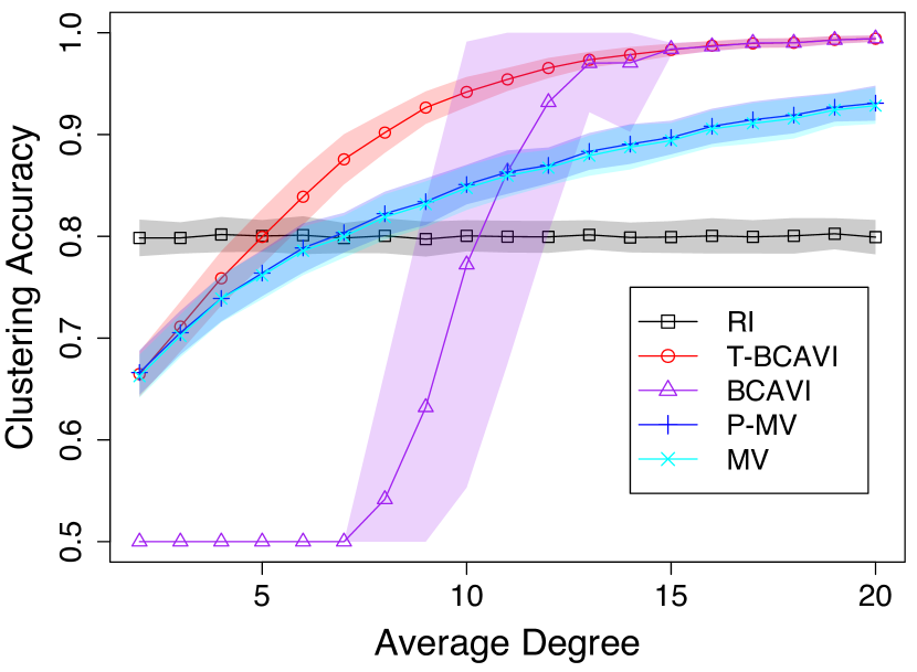
(a) $\varepsilon=0.2$, $n_{1}=n_{2}=300$

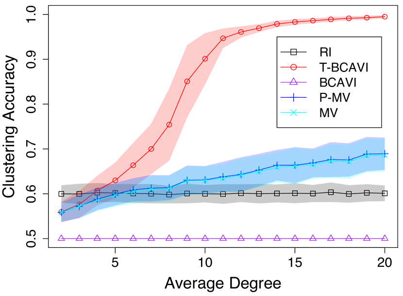
(b) $\varepsilon=0.4$, $n_{1}=n_{2}=300$

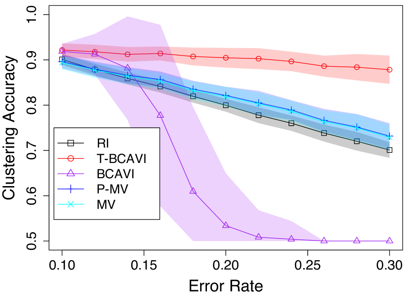
(c) $d=8$, $n_{1}=n_{2}=300$

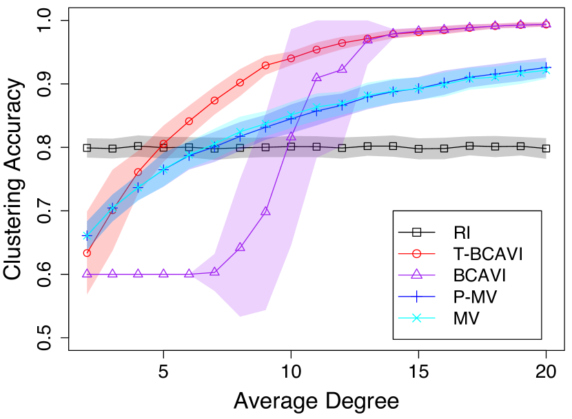
(d) $\varepsilon=0.2$, $n_{1}=240$, $n_{2}=360$

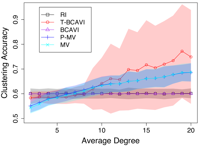
(e) $\varepsilon=0.4$, $n_{1}=240$, $n_{2}=360$

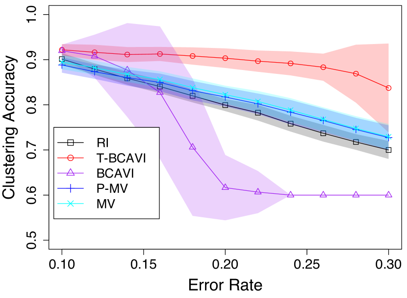
(f) $d=8$, $n_{1}=240$, $n_{2}=360$

Figure 1: Performance of Threshold BCAVI (T-BCAVI), the classical BCAVI, majority vote (MV), and majority vote with penalization (P-MV) in different settings. Networks are generated from SBM with $n=600$ nodes, $K=2$ communities of sizes $n_{1}$ and $n_{2}$, $p/q=10/3$, and average degree $d=((n_{1}^{2}+n_{2}^{2})p+2n_{1}n_{2}q)/n$. Initializations are generated from true node labels according to Assumption 3.1 with error rate $\varepsilon$, resulting in actual clustering initialization accuracy (RI) of approximately $1-\varepsilon$.

In addition, we supply experimental results for the accuracy of parameter estimation. We report the relative errors of $p^{(s)}$, $q^{(s)}$ and $p^{(s)}/q^{(s)}$, defined by $\frac{p^{(s)}-p}{p}$, $\frac{q^{(s)}-q}{q}$, and $\frac{p^{(s)}/q^{(s)}-p/q}{p/q}$, respectively. Figure 2(a) shows that, overall, T-BCAVI is much more accurate than BCAVI in parameter estimation for sparse networks. Both algorithms overestimate $q$ and underestimate $p$, although the bias is smaller for T-BCAVI. When the network is dense, two algorithms have a negligible relative error. Figure 2(b) shows that when the initialization contains a large amount of wrong labels ($\varepsilon=0.4$), T-BCAVI still provides meaningful estimates of $p$ and $q$ while the estimation errors of BCAVI do not reduce as the average degree increases. This is because BCAVI always produces $p^{(s)}=q^{(s)}$ when $s$ is sufficiently large. Figure 2(c) further confirms that T-BCAVI is much more robust with respect to initialization than BCAVI is.

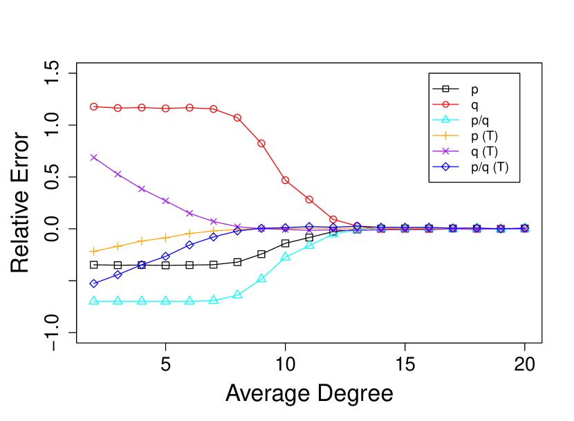
(a) $\varepsilon=0.2$

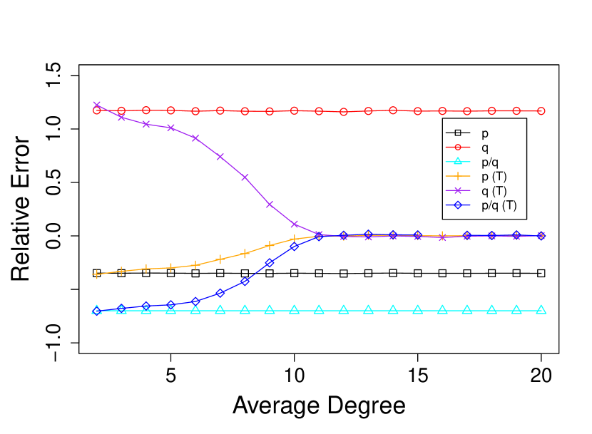
(b) $\varepsilon=0.4$

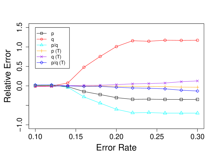
(c) $d=8$

Figure 2: Relative errors of parameter estimation by Threshold BCAVI (T) and the classical BCAVI in different settings. Networks are generated from SBM with $n=600$ nodes, $K=2$ communities of equal sizes, $p/q=10/3$, and average degree $d=n(p+q)/2$. Initializations are generated from true node labels according to Assumption 3.1 with error rate $\varepsilon$.

(b) Two communities with initialization by spectral clustering. Since the initialization in Assumption 3.1 is not available in practice, we now evaluate the performance of all methods using initialization generated from network data splitting (Chin et al., 2015; Li et al., 2020). According to the discussion in Section 2, we fix a sampling probability $\tau\in(0,1/2)$ and sample edges in $A$ independently with probability $\tau$; denote by $A^{(\text{init})}$ the adjacency matrix of the resulting sampled network. To get a warm initialization $Z^{(0)}$, we apply spectral clustering algorithm (Von Luxburg, 2007) on $A^{(\text{init})}$. All methods are then performed on the remaining sub-network $A-A^{(\text{init})}$ using the initialization $Z^{(0)}$. For reference, we also report the accuracy of $Z^{(0)}$ (SCI).

Similar to the previous setting when $Z^{(0)}$ are generated according to Assumption 3.1, Figure 3 shows that T-BCAVI performs much better than other methods for both balanced and unbalanced networks, especially when the spectral clustering initialization is almost uninformative (accuracy close to random guess of 1/2 when the network is balanced). This observation again highlights that T-BCAVI often requires a much weaker initialization than what BCAVI and variants of majority vote need. Network data splitting also provides a practical way to implement our algorithm in the real-world data analysis.

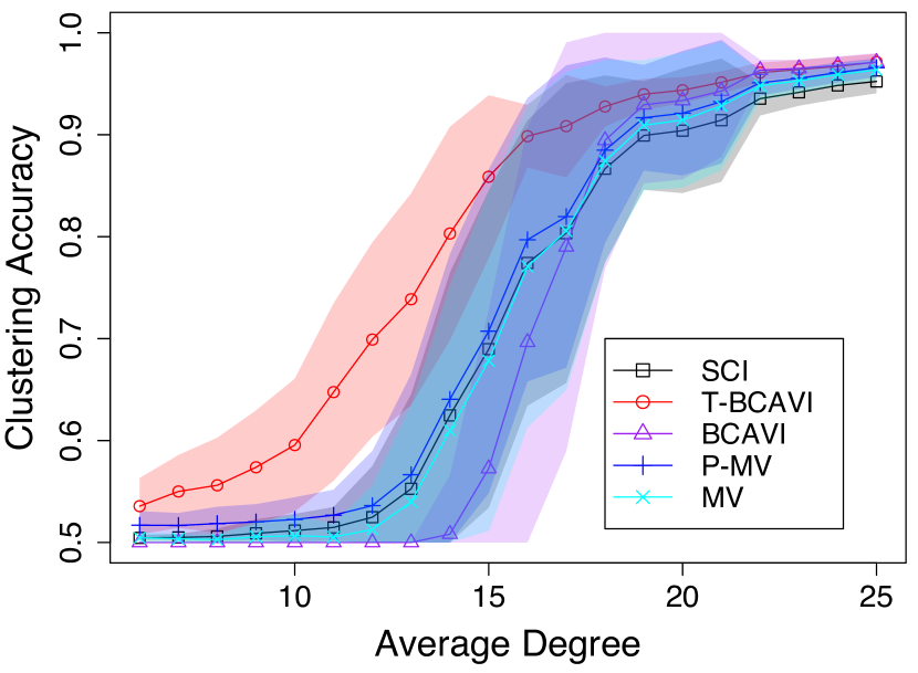
(a) $\tau=0.5$, $n_{1}=n_{2}=300$

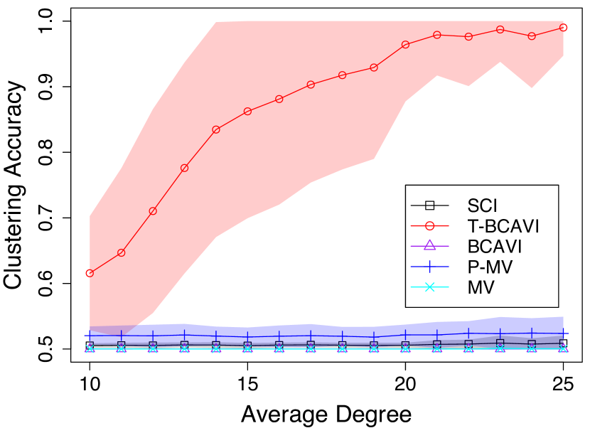
(b) $\tau=0.2$, $n_{1}=n_{2}=300$

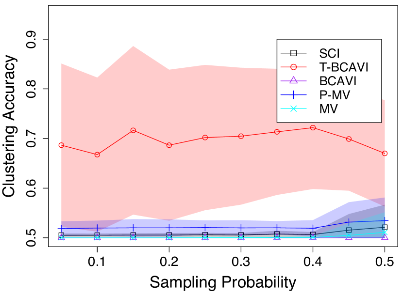
(c) $d=12$, $n_{1}=n_{2}=300$

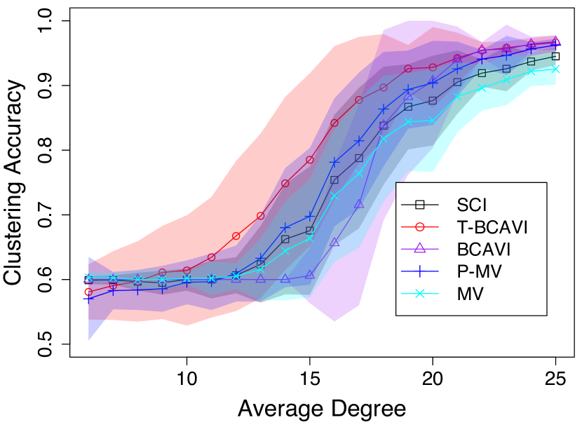
(d) $\tau=0.5$, $n_{1}=240$, $n_{2}=360$

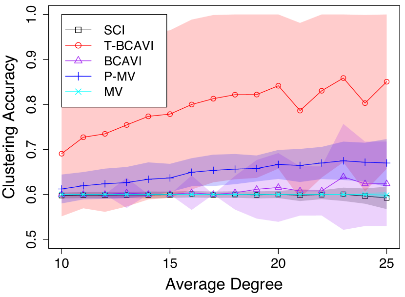
(e) $\tau=0.2$, $n_{1}=240$, $n_{2}=360$

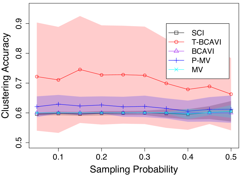
(f) $d=12$, $n_{1}=240$, $n_{2}=360$

Figure 3: Performance of Threshold BCAVI (T-BCAVI), the classical BCAVI, majority vote (MV), and majority vote with penalization (P-MV) in different settings. Networks are generated from SBM with $n=600$ nodes, $K=2$ communities of sizes $n_{1}$ and $n_{2}$, $p/q=10/3$, and average degree $d=((n_{1}^{2}+n_{2}^{2})p+2n_{1}n_{2}q)/n$. Initializations are computed by spectral clustering (SCI) applied to sampled sub-networks $A^{(\text{init})}$ with sampling probability $\tau$ while T-BCAVI and BCAVI are performed on remaining sub-networks $A-A^{(\text{init})}$.

Figure 4(a) further shows that T-BCAVI outperforms BCAVI in estimating the model parameters of sparse networks. When the average degree is large, both algorithms have the similar and negligible errors. This is consistent with the results in Figure 2(a) and 2(b) when initialization are generated according to Assumption 3.1. Figure 4(b) shows a much better improvement of T-BCAVI over BCAVI; this is because $\tau=0.2$ (compared to $\tau=0.5$ in Figure 4(a)), indicating that the initialization is poor due to the sparsity of the sub-network $A^{(\text{init})}$ to which spectral clustering is applied. Figure 4(c) further confirms that T-BCAVI is more robust than BCAVI with respect to the sampling probability $\tau$.

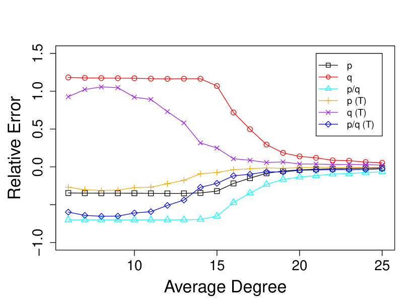
(a) $\tau=0.5$

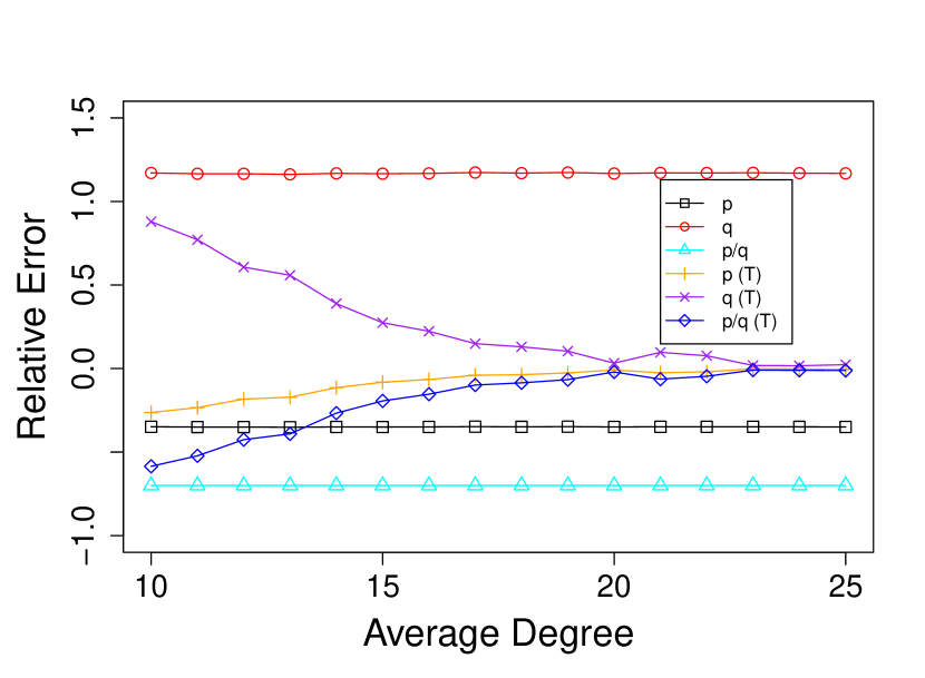
(b) $\tau=0.2$

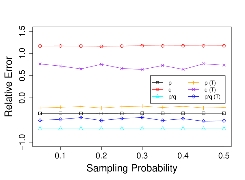
(c) $d=12$

Figure 4: Relative errors of parameter estimation by Threshold BCAVI (T) and the classical BCAVI in different settings. Networks are generated from SBM with $n=600$ nodes, $K=2$ communities of equal sizes, $p/q=10/3$, and average degree $d=n(p+q)/2$. Initializations are computed by spectral clustering (SCI) applied to sampled sub-networks $A^{(\text{init})}$ with sampling probability $\tau$ while T-BCAVI and BCAVI are performed on remaining sub-networks $A-A^{(\text{init})}$.

(c) Three communities with idealized and spectral clustering initializations. Although our theoretical guarantees are only for SBM with two communities, we emphasize that T-BCAVI can be carried out for any SBM, as described in Section 2. To that end, we now consider SBM with $n=600$ nodes, $K=3$ communities of sizes $n_{1}$, $n_{2}$, $n_{3}$, and the block probability matrix given by

$$B=\begin{pmatrix}p&q&q\\ q&p&q\\ q&q&p\end{pmatrix},$$

where the ratio $p/q$ is fixed to be 10/3. The measure of accuracy for estimated labels in the setting $K=2$ can be extended to the case $K=3$ in a natural way. Note, however, that choosing node labels independently and uniformly at random now results in the baseline accuracy of approximately $1/3$ in the balanced network. Figures 5(a) and 5(c) show the performance of all methods using initializations generated according to Assumption 3.1 with error rate $\varepsilon=0.4$; Figures 5(b) and 5(d) show the case when these methods use initializations computed by spectral clustering with sampling probability $\tau=0.25$. Similar to the case of the two communities, T-BCAVI does not require accurate initializations and completely outperforms other methods for both balanced and unbalanced networks.

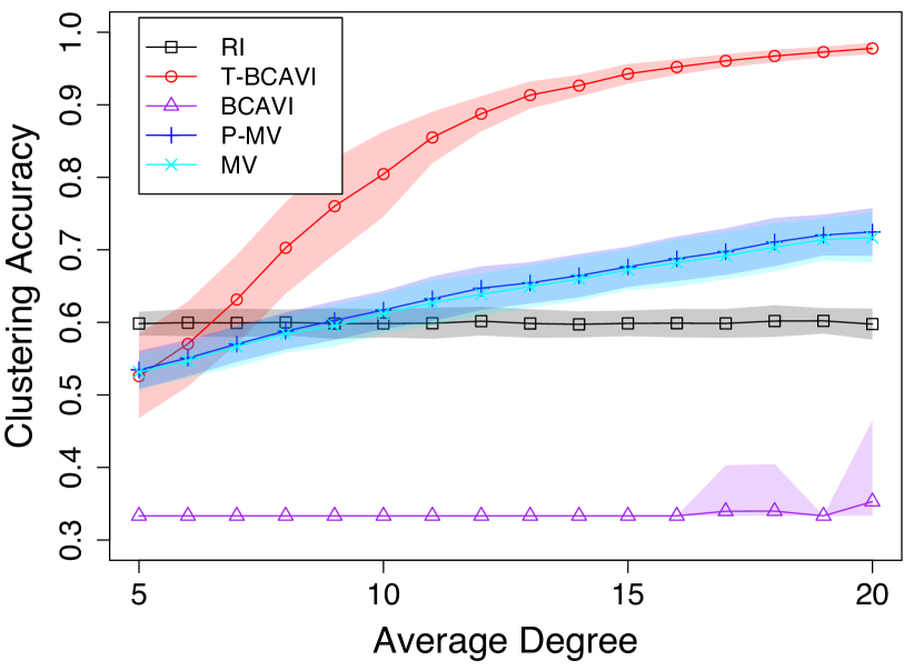
(a) $\varepsilon=0.4$, $n_{1}=n_{2}=n_{3}=200$

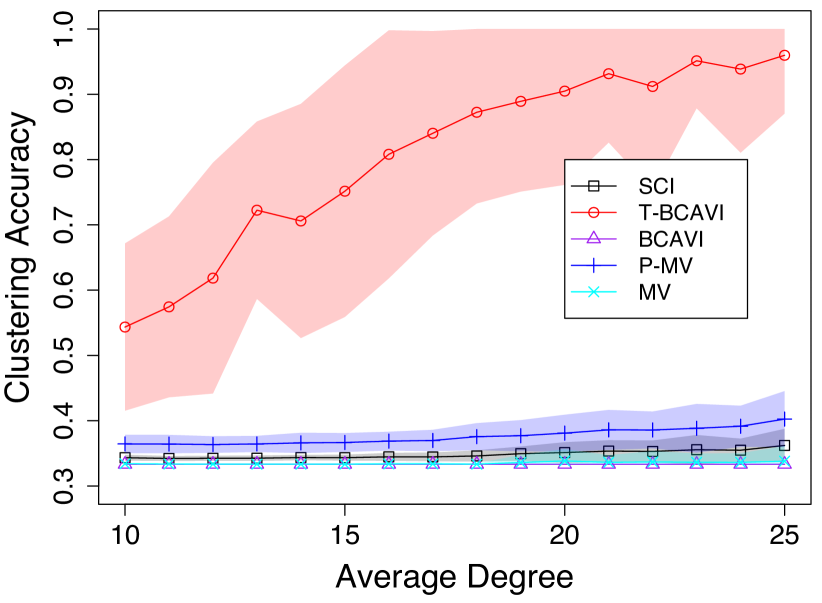
(b) $\tau=0.25$, $n_{1}=n_{2}=n_{3}=200$

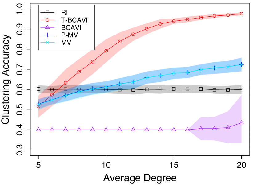
(c) $\varepsilon=0.4$, $n_{1}=150$, $n_{2}=210$, $n_{3}=240$

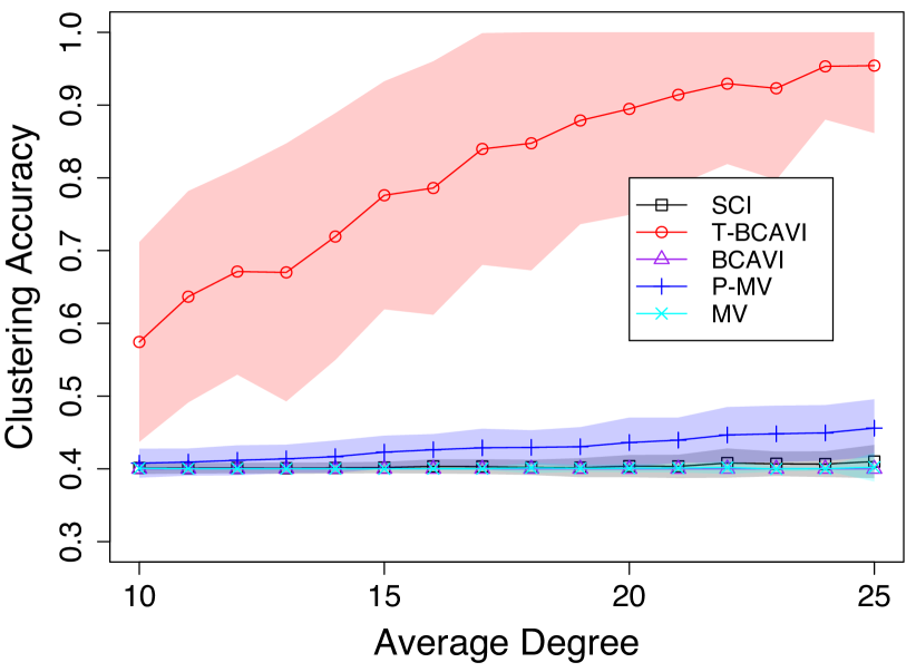
(d) $\tau=0.25$, $n_{1}=150$, $n_{2}=210$, $n_{3}=240$

Figure 5: Performance of Threshold BCAVI (T-BCAVI), the classical BCAVI, majority vote (MV), and majority vote with penalization (P-MV) in different settings. Networks are generated from SBM with $n=600$ nodes, $K=3$ communities of sizes $n_{1}$, $n_{2}$ and $n_{3}$, $p/q=10/3$, and average degree $d=((n_{1}^{2}+n_{2}^{2}+n_{3}^{2})p+2(n_{1}n_{2}+n_{2}n_{3}+n_{3}n_{1})q)/n$. Plots (a) and (c): Initializations are generated from true node labels according to Assumption 3.1 with error rate $\varepsilon=0.4$. Plots (b) and (d): Initializations are computed by spectral clustering (SCI) applied to sampled sub-networks $A^{(\text{init})}$ with sampling probability $\tau=0.25$ while T-BCAVI and BCAVI are performed on remaining sub-networks $A-A^{(\text{init})}$.

4.2 Real Data Examples

We first consider the political blogosphere network data set (Adamic and Glance, 2005). It is related to the 2004 U.S. presidential election, where the nodes are blogs focused on American politics and the edges are hyperlinks connecting the blogs. These blogs have been labeled manually as either “liberal” or “conservative” (Adamic and Glance, 2005). We ignore the direction of the hyperlinks and conduct our analysis on the largest connected component of the network (Karrer and Newman, 2011), which contains 1490 nodes, and the average node degree is 22.44. This network includes 732 conservative blogs and 758 liberal blogs.

Another political data set, which is also related to the 2004 presidential election, is a network of books about US politics published around the 2004 presidential election and sold by the online bookseller Amazon.com. Edges between books represent frequent co-purchasing of books by the same buyers. The network was compiled by Krebs (2022) and was posted by Newman (2013). The books are labeled as ”liberal,” ”neutral,” or ”conservative” based on their descriptions and reviews of the books (Newman, 2013). This network has an average degree of 8.40, and it contains 49 conservative books, 43 liberal books, and 13 neutral books.

The last data set we analyze in this section is the network of common adjectives and nouns in the novel “David Copperfield” by Charles Dickens, as described by Newman (2006). Nodes represent the most commonly occurring adjectives and nouns in the book. Node labels are 0 for adjectives and 1 for nouns. Edges connect any pair of words that occur in an adjacent position in the text of the book. The network has 58 adjectives and 54 nouns with an average degree of 7.59.

Similar to Section 4.1, to implement all methods, we first randomly sample a sub-network and apply spectral clustering algorithm to get a warm initialization. We then run these algorithms on the remaining sub-network for comparison. Figure 6(a) for political blogosphere shows that they all improve the accuracy of the initialization, but T-BCAVI outperforms other methods for almost all sampling probability $\tau$. Figure 6(b) for the book network shows that BCAVI, MV, and P-MV do not improve the initialization much while T-BCAVI still improves the accuracy of the initialization considerably. Finally, Figure 6(c) shows that T-BCAVI is still consistently better than other methods, although the initializations are close to the random guess, resulting in a small improvement of all algorithms.

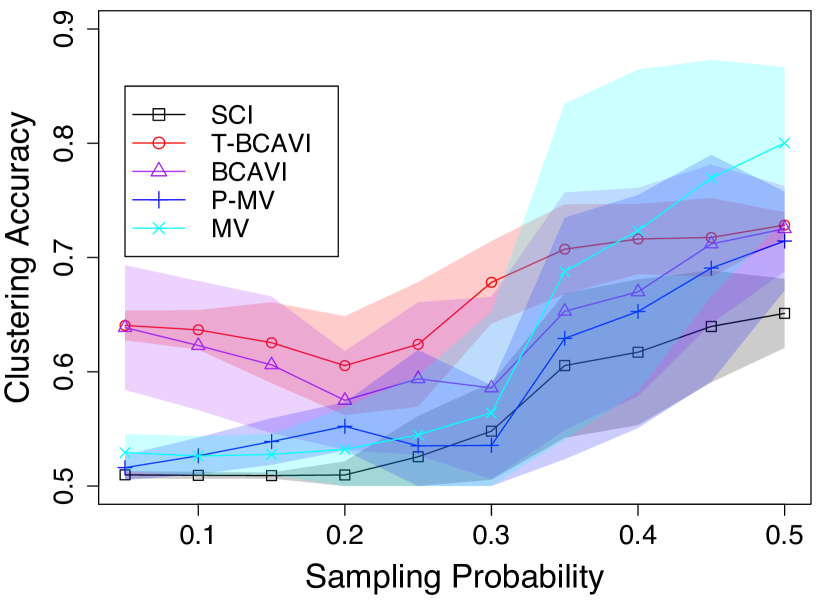
(a) Politics blogosphere (K=2)

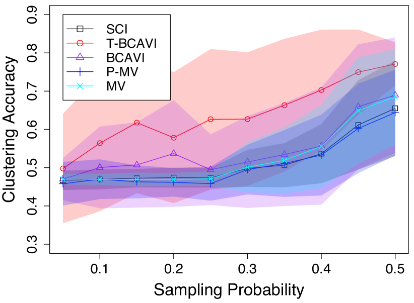
(b) Politics book (K=3)

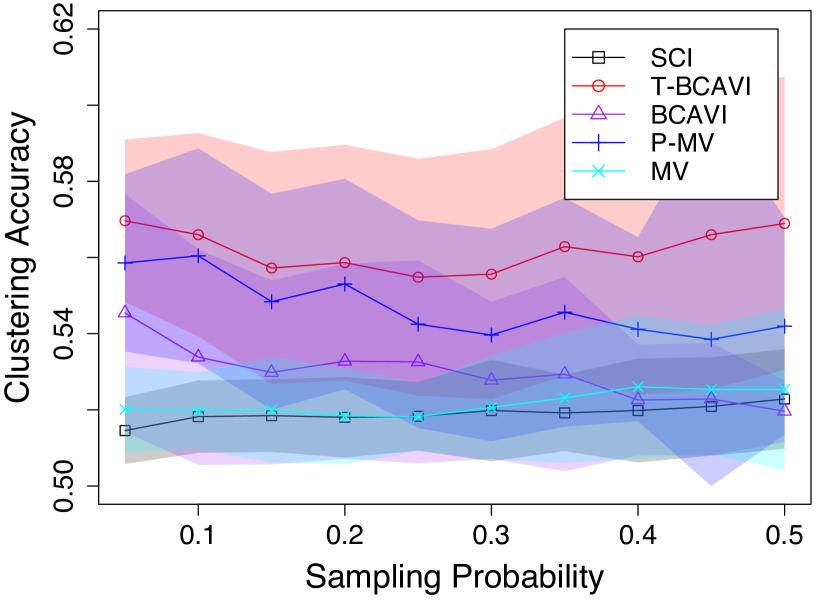
(c) Adjectives and nouns (K=2)

Figure 6: Performance of regularized BCAVI (T-BCAVI) and the classical BCAVI in real data examples. Initializations are computed by spectral clustering (SCI) applied to sampled sub-networks $A^{(\text{init})}$ with sampling probability $\tau$ while T-BCAVI and BCAVI are performed on remaining sub-networks $A-A^{(\text{init})}$. Plot (a): Two communities of sizes 732 and 758. Plot (b): Three communities of sizes 49, 43, and 13. Plot (c): Two communities of sizes 58 and 54.

5 Discussion

This paper studies the batch coordinate update variational inference algorithm for community detection under the stochastic block model. Existing work in this direction only establishes the theoretical support for this iterative algorithm in the relatively dense regime. The contribution of this paper is two-fold. First, we extend the validity of the variational approach to the sparse setting when node degrees may be bounded. Second, we propose a simple but novel threshold strategy that significantly improves the accuracy of the classical variational inference method, especially in the sparse regime or when the accuracy of the initialization is poor.

While we only have theoretical results for the stochastic block model with two communities, we believe that similar results also hold for more general settings and leave their analysis for future work. In addition, Assumption 3.1 requires that each entry of the initialization is perturbed independently with the same error rate. Simulations in Section 4 suggest that our algorithm works for much weaker assumptions on the initialization.

Finally, extending our results beyond stochastic block models and network problems is a promising research direction. For example, the numerical results for Gaussian mixtures in Appendix B show that the improvement of the threshold step is not network-specific. Obtaining theoretical results for this setting is the first step in the direction we plan to pursue.

Appendix A Proofs of Results in Section 3

Let us first recall the updates of $\Psi^{(s)}$ and $\xi^{(s)}$ described in Section 3:

$$\Psi^{(s)}=h\big{(}\xi^{(s)}\big{)},\quad\xi^{(s)}=4t^{(s)}\left(A-\lambda^{(s)}(\mathbf{1}_{n}\mathbf{1}_{n}^{T}-I_{n})\right)\left(\Psi^{(s-1)}-1/2\cdot\mathbf{1}_{n}\right),\quad s\geq 1.$$ (A6)

To analyze the threshold BCAVI, we consider the population version of $\xi^{(s)}$, following Sarkar et al. (2021):

$$\bar{\xi}^{(s)}:=4t^{(s)}M^{(s)}\left(\Psi^{(s-1)}-1/2\cdot\mathbf{1}_{n}\right),$$ (A7)

where $M^{(s)}:=P-\lambda^{(s)}(\mathbf{1}_{n}\mathbf{1}_{n}^{T}-I_{n})$ and $P=\mathbb{E}[A|Z]$ is a $2\times 2$ block matrix with constant values $p$ or $q$ within each block. A direct calculation shows that eigenvalues of $M^{(s)}$ are

$$\nu_{1}^{(s)}=n\left(\frac{p+q}{2}-\lambda^{(s)}\right)-(p-\lambda^{(s)}),\quad\nu_{2}=\frac{n(p-q)}{2}-(p-\lambda^{(s)}),\quad\nu_{i}^{(s)}=-(p-\lambda^{(s)}),\quad i\geq 3.$$

The corresponding eigenvectors for $\nu_{1}^{(s)}$ and $\nu_{2}^{(s)}$ are $u_{1}=\mathbf{1}_{n}$ and $u_{2}=\mathbf{1}_{\mathcal{C}_{1}}-\mathbf{1}_{\mathcal{C}_{2}}$, respectively. We decompose $\Psi^{(s)}$ according to these eigenvectors as

$$\Psi^{(s)}=\zeta_{1}^{(s)}u_{1}+\zeta_{2}^{(s)}u_{2}+v^{(s)},$$ (A8)

where

$$\zeta_{i}^{(s)}=\langle\Psi^{(s)},u_{i}\rangle/n,\quad i=1,2.$$ (A9)

Formula (A8) yields the following coordinate-wise version of (A7):

$$\bar{\xi}_{i}^{(s)} = 4t^{(s)}n\left[\left(\zeta_{1}^{(s-1)}-\frac{1}{2}\right)\left(\frac{p+q}{2}-\lambda^{(s)}\right)+\sigma_{i}\zeta_{2}^{(s-1)}\frac{p-q}{2}\right]$$ (A10)

$$+4t^{(s)}\left(\lambda^{(s)}-p\right)\left[\left(\zeta_{1}^{(s-1)}-\frac{1}{2}\right)+\sigma_{i}\zeta_{2}^{(s-1)}+v^{(s-1)}_{i}\right]$$

$$=: na_{\sigma_{i}}^{(s-1)}+b_{i}^{(s-1)}.$$

Unlike Sarkar et al. (2021), we need to control the irregularity of sparse networks carefully. To that end, denote by $A^{\prime}$ the adjacency matrix of the network obtained from the observed network by removing some edges (in an arbitrary way) of nodes with degrees greater than $C_{0}d$ so that all node degrees of the new network are at most $C_{0}d$, where $C_{0}>0$ is a fixed constant. Note that $A^{\prime}$ is only used for the proofs, and our algorithm does not need to specify it.

In the following lemmas, we assume that the assumptions of Proposition 1 and Theorem 2 are satisfied.

Lemma 4 (Number of removed edges)

Assume that $\kappa\leq d\leq\eta\log n$ for a large constant $\kappa>0$ and a constant $\eta\in(0,1)$. Then with high probability, we have

$$\sum_{i,j}(A_{ij}-A_{ij}^{\prime})\leq 2n\exp(-c_{0}d),$$

where $c_{0}$ is an absolute constant.

Proof [of Lemma 4] It follows from Proposition 1.12 of Benaych-Georges et al. (2019) that with high probability,

$$\sum_{i,j}(A_{ij}-A^{\prime}_{ij})\leq 2\sum_{k=C_{0}d+1}^{\infty}kn\exp(-f(k)),$$

where

$$f(x)=x\log\left(\frac{x}{d}\right)-(x-d)-\log\sqrt{2\pi x}.$$

Notice that for $k>C_{0}d$,

$$f(k)-\log k\geq k(\log C_{0}-1)-\log\sqrt{2\pi k}-\log k\geq k(\log C_{0}-1)/2.$$

This implies the following inequality

$$\sum_{i,j}(A_{ij}-A^{\prime}_{ij})\leq 2n\sum_{k=C_{0}d+1}^{\infty}\exp\left(-\frac{\log C_{0}-1}{2}k\right)\leq 2n\exp(-c_{0}d)$$

occurs with high probability for some constant $c_{0}$.  

Lemma 5 (Concentration of regularized adjacency matrices)

Let $P=\mathbb{E}[A|Z]$. With high probability,

$$||A^{\prime}-\mathbb{E}A||=O(\sqrt{d}),$$

where $\|.\|$ denotes the spectral norm.

Proof [of Lemma 5] This lemma is a special case of Theorem 1.1 in Le et al. (2017).  

The next lemma provides crude bounds for the parameters of the threshold BCAVI after the first iteration.

Lemma 6 (First step: Parameter estimation)

Fix $\varepsilon\in(0,1/2)$ and consider an initialization for the threshold BCAVI that satisfies Assumption 3.1. Then there exist positive constants $C,C_{1},C_{2}$ only depending on $\varepsilon$ such that if $d=n(p+q)/2>C$ then with high probability,

$$t^{(1)}\geq C_{1},\quad\Big{|}\lambda^{(1)}-\frac{p+q}{2}\Big{|}\leq C_{2}\rho_{n}.$$

Proof [of Lemma 6] Recall the first update $p^{(1)}$ described in Section 3:

$$p^{(1)}=\frac{(Z^{(0)})^{T}AZ^{(0)}+(\mathbf{1}_{n}-Z^{(0)})^{T}A(\mathbf{1}_{n}-Z^{(0)})}{(Z^{(0)})^{T}(J_{n}-I_{n})Z^{(0)}+(\mathbf{1}_{n}-Z^{(0)})^{T}(J_{n}-I_{n})(\mathbf{1}_{n}-Z^{(0)})},$$

where $J_{n}=\mathbf{1}_{n}\mathbf{1}_{n}^{T}$. We first analyze the denominator of $p^{(1)}$.

Since $Z^{(0)}$ satisfies Assumption 3.1, it follows that $\sum_{i}Z^{(0)}_{i}=n/2+O_{P}(\sqrt{n})$ by the standard Chernoff bound. Therefore, the denominator of $p^{(1)}$ can be approximated as follows. First,

$${Z^{(0)}}^{T}(J_{n}-I_{n})Z^{(0)} =\sum_{i\neq j}Z^{(0)}_{i}Z^{(0)}_{j}=\left(\sum_{i=1}^{n}Z^{(0)}_{i}\right)^{2}-\sum_{i=1}^{n}(Z^{(0)}_{i})^{2}$$

$$=\left(\sum_{i=1}^{n}Z^{(0)}_{i}\right)^{2}-\sum_{i=1}^{n}Z^{(0)}_{i}=n^{2}/4+O_{P}(n^{3/2}).$$

Similarly,

$$(\mathbf{1}_{n}-Z^{(0)})^{T}(J_{n}-I_{n})(\mathbf{1}_{n}-Z^{(0)})=n^{2}/4+O_{P}(n^{3/2}).$$

These estimates give

$$(Z^{(0)})^{T}(J_{n}-I_{n})Z^{(0)}+(\mathbf{1}_{n}-Z^{(0)})^{T}(J_{n}-I_{n})(\mathbf{1}_{n}-Z^{(0)})=n^{2}/2+O_{p}(n^{3/2}).$$ (A11)

By replacing $A$ with $P+(A-P)$, we decompose the numerator of $p^{(1)}$ as the sum of signal and noise terms:

signal $$:= (Z^{(0)})^{T}PZ^{(0)}+(\mathbf{1}_{n}-Z^{(0)})^{T}P(\mathbf{1}_{n}-Z^{(0)}),$$

noise $$:= (Z^{(0)})^{T}(A-P)Z^{(0)}+(\mathbf{1}_{n}-Z^{(0)})^{T}(A-P)(\mathbf{1}_{n}-Z^{(0)}).$$

Again, by Assumption 3.1 and the Chernoff bound,

$$\sum_{i\in\mathcal{C}_{1}}Z^{(0)}_{i}=n(1-\varepsilon)/2+O_{P}(\sqrt{n}),\quad\sum_{i\in\mathcal{C}_{2}}Z^{(0)}_{i}=n\varepsilon/2+O_{P}(\sqrt{n}).$$

Therefore,

$$(Z^{(0)})^{T}PZ^{(0)} = \left[\left(\sum_{i\in\mathcal{C}_{1}}Z^{(0)}_{i}\right)^{2}-\sum_{i\in\mathcal{C}_{1}}(Z^{(0)}_{i})^{2}+\left(\sum_{i\in\mathcal{C}_{2}}Z^{(0)}_{i}\right)^{2}-\sum_{i\in\mathcal{C}_{2}}(Z^{(0)}_{i})^{2}\right]p$$

$$+2\left[\left(\sum_{i\in\mathcal{C}_{1}}Z^{(0)}_{i}\right)\left(\sum_{i\in\mathcal{C}_{2}}Z^{(0)}_{i}\right)\right]q$$

$$= \left[n^{2}(1-\varepsilon)^{2}/4+n^{2}\varepsilon^{2}/4\right]p+\left[n^{2}\varepsilon(1-\varepsilon)/2\right]q+O_{P}(n^{3/2}\rho_{n}).$$

Using a similar estimate for $(\mathbf{1}_{n}-Z^{(0)})^{T}P(\mathbf{1}_{n}-Z^{(0)})$, we get

$$\text{signal}=\left(\frac{n^{2}[\varepsilon^{2}+(1-\epsilon)^{2}]}{2}\right)p+[n^{2}\varepsilon(1-\varepsilon)]q+O_{P}(n^{3/2}\rho_{n}).$$ (A12)

We now analyze the noise term. Since

$$\mathbb{E}[(Z^{(0)})^{T}(A-P)Z^{(0)}|Z^{(0)}]=0,$$

we have

$$\text{Var}[(Z^{(0)})^{T}(A-P)Z^{(0)}] =\mathbb{E}\left[\text{Var}[(Z^{(0)})^{T}(A-P)Z^{(0)}|Z^{(0)}]\right]$$

$$=4\mathbb{E}\left[\sum_{i<j}Z^{(0)}_{i}Z^{(0)}_{j}\text{Var}[A_{ij}]\right]\leq 2n^{2}p.$$

By Chebyshev’s inequality,

$$(Z^{(0)})^{T}(A-P)Z^{(0)}=O_{P}(n\sqrt{\rho_{n}}).$$

Similarly,

$$(\mathbf{1}_{n}-Z^{(0)})^{T}(A-P)(\mathbf{1}_{n}-Z^{(0)})=O_{P}(n\sqrt{\rho_{n}}).$$

These bounds give

$$\text{noise}=O_{P}(n\sqrt{\rho_{n}}).$$ (A13)

From (A11), (A12), and (A13) we get

$$p^{(1)}=p-2\varepsilon(1-\varepsilon)(p-q)+O_{P}(\rho_{n}/\sqrt{n}).$$ (A14)

A similar analysis gives

$$q^{(1)}=q+2\varepsilon(1-\varepsilon)(p-q)+O_{P}(\rho_{n}/\sqrt{n}).$$ (A15)

Since

$$t^{(1)}=\frac{1}{2}\log\frac{p^{(1)}(1-q^{(1)})}{q^{(1)}(1-p^{(1)})},\quad\lambda^{(1)}=\frac{1}{2t^{(1)}}\log\frac{1-q^{(1)}}{1-p^{(1)}},$$

it follows from (A14) and (A15) that

$$t^{(1)}\geq C_{1},\quad\Big{|}\lambda^{(1)}-\frac{p+q}{2}\Big{|}\leq C_{2}\rho_{n}$$

with high probability for some constants $C_{1}$, $C_{2}$ only depending on $\varepsilon$. The proof is complete.  

The next lemma provides the accuracy of the label estimates after the first iteration.

Lemma 7 (First step: Label estimation)

With high probability,

$$||\Psi^{(1)}-\mathbf{1}_{\mathcal{C}_{1}}||_{1}\leq n\exp(-cd),$$

where $c$ is a constant only depending on $\varepsilon$.

Proof [of Lemma 7] According to the population update in (A10) with $s=1$, we have

$$\bar{\xi}_{i}^{(1)} = 4t^{(1)}n\left[\left(\zeta_{1}^{(0)}-\frac{1}{2}\right)\left(\frac{p+q}{2}-\lambda^{(1)}\right)+\sigma_{i}\zeta_{2}^{(0)}\frac{p-q}{2}\right]$$ (A16)

$$+4t^{(1)}\left(\lambda^{(1)}-p\right)\left[\left(\zeta_{1}^{(0)}-\frac{1}{2}\right)+\sigma_{i}\zeta_{2}^{(0)}+v^{(0)}_{i}\right]$$

$$=: na_{\sigma_{i}}^{(0)}+b_{i}^{(0)},$$

where $\sigma_{i}=1$ if $i\in\mathcal{C}_{1}$ and $\sigma_{i}=-1$ otherwise, and according to (A9),

$$\zeta_{1}^{(0)} = (Z^{(0)})^{T}\mathbf{1}_{n}/n=1/2+O_{p}(1/\sqrt{n}),$$

$$\zeta_{2}^{(0)} = (Z^{(0)})^{T}(\mathbf{1}_{\mathcal{C}_{1}}-\mathbf{1}_{\mathcal{C}_{2}})/n=(1-2\varepsilon)/2+O_{p}(1/\sqrt{n}).$$ (A17)

It follows from (A16), (A) and Lemma 6 that $na_{\sigma_{i}}^{(0)}=\Omega(n\rho_{n})$ and $b_{i}^{(0)}=O(\rho_{n})$ with high probability. Moreover, the dominated term of $na_{\sigma_{i}}^{(0)}$ is $nt^{(1)}\sigma_{i}(1-2\varepsilon)(p-q)$.

Returning to the sample updates in (A6) with $s=1$, we have

$$\xi^{(1)}_{i}=na_{\sigma_{i}}^{(0)}+b_{i}^{(0)}+4t^{(1)}r_{i}^{(0)},$$

where the error term $r_{i}^{(0)}$ is

$$r_{i}^{(0)}=\sum_{j\neq i}(A_{ij}-P_{ij})(Z_{j}^{(0)}-1/2).$$

To show the accuracy of $\Psi_{i}^{(1)}$, we will prove that the noise level $|4t^{(1)}r_{i}^{(0)}|$ is small compared to the signal strength $nt^{(1)}(1-2\varepsilon)(p-q)$ in the population update. To this end, we claim that node $i$ is correctly labeled if

$$|r_{i}^{(0)}|<\frac{(1-2\varepsilon)(p-q)}{2(p+q)}d.$$

Let $Y_{ij}=(A_{ij}-P_{ij})(Z_{j}^{(0)}-1/2)$, $\delta$ be a constant such that $0<\delta<\frac{(1-2\varepsilon)(p-q)}{2(p+q)}$, and $\{Y_{ij}^{*}\}$ be an independent copy of $\{Y_{ij}\}$. For an event $E$, denote by $\mathbbm{1}(E)$ the indicator of $E$. Then by the triangle inequality,

$$\mathbbm{1}\big{(}|r_{i}^{(0)}|>\delta d\big{)} =\mathbbm{1}\Big{(}|\sum_{j\neq i}Y_{ij}|>\delta d\Big{)}\leq\mathbbm{1}\Big{(}\Big{|}\sum_{j=1}^{i-1}Y_{ij}\Big{|}+\Big{|}\sum_{j=i+1}^{n}Y_{ij}\Big{|}>\delta d\Big{)}$$

$$\leq\mathbbm{1}\Big{(}\Big{|}\sum_{j=1}^{i-1}Y_{ij}\Big{|}+\Big{|}\sum_{j=i+1}^{n}Y_{ij}\Big{|}+\Big{|}\sum_{j=1}^{i-1}Y_{ij}^{*}\Big{|}+\Big{|}\sum_{j=i+1}^{n}Y_{ij}^{*}\Big{|}>\delta d\Big{)}$$

$$\leq\mathbbm{1}\Big{(}\Big{|}\sum_{j=1}^{i-1}Y_{ij}\Big{|}+\Big{|}\sum_{j=i+1}^{n}Y_{ij}^{*}\Big{|}>\frac{\delta d}{2}\Big{)}+\mathbbm{1}\Big{(}\Big{|}\sum_{j=1}^{i-1}Y_{ij}^{*}\Big{|}+\Big{|}\sum_{j=i+1}^{n}Y_{ij}\Big{|}>\frac{\delta d}{2}\Big{)}.$$

Applying Bernstein’s inequality for $\{Y_{ij}\}$ with $\mathbb{E}[Y_{ij}]=0$, $|Y_{ij}|<1/2$ and $\mathbb{E}[Y_{ij}^{2}]\leq p/4$, we get

$$\mathbb{P}\Big{(}\Big{|}\sum_{j=1}^{i-1}Y_{ij}\Big{|}+\Big{|}\sum_{j=i+1}^{n}Y_{ij}^{*}\Big{|}>\frac{\delta d}{2}\Big{)} \leq\mathbb{P}\Big{(}\Big{|}\sum_{j=1}^{i-1}Y_{ij}\Big{|}>\frac{\delta d}{4}\Big{)}+\mathbb{P}\Big{(}\Big{|}\sum_{j=i+1}^{n}Y_{ij}^{*}\Big{|}>\frac{\delta d}{4}\Big{)}$$

$$\leq 4\exp\left(\frac{-(\delta d/4)^{2}/2}{d/2+(\delta d/4)/6}\right)=4\exp\left(\frac{-\delta^{2}d}{16+4\delta/3}\right).$$

Since $(\sum_{j=1}^{i-1}Y_{ij},\sum_{j=i+1}^{n}Y_{ij}^{*})$, $1\leq i\leq n$, are independent, by Bernstein’s inequality,

$$\sum_{i=1}^{n}\mathbbm{1}\Big{(}\Big{|}\sum_{j=1}^{i-1}Y_{ij}\Big{|}+\Big{|}\sum_{j=i+1}^{n}Y_{ij}^{*}\Big{|}>\frac{\delta d}{2}\Big{)}\leq 4(1+o(1))n\exp\left(\frac{-\delta^{2}d}{16+4\delta/3}\right)$$

with probability at least $1-n^{-r}$ for some constant $r>0$. Therefore, the following event

$$\mathcal{A}_{1}=\left\{\sum_{i=1}^{n}\mathbbm{1}(|r_{i}^{(0)}|>\delta d)\leq 8(1+o(1))n\exp\left(\frac{-\delta^{2}d}{16+4\delta/3}\right)\right\}$$

occurs with high probability. Clearly, $\mathcal{A}_{1}$ implies $||\Psi^{(1)}-\mathbf{1}_{\mathcal{C}_{1}}||_{1}\leq n\exp(-cd)$ for some constant $c$ only depending on $\varepsilon$.  

Using the bound for $\Psi^{(1)}$ in Lemma 7, we now provide estimates for parameters of the threshold BCAVI in the second iteration.

Lemma 8 (Second step: Parameter estimation)

With high probability,

$$|p^{(2)}-p|\leq p\exp(-cd), \quad|q^{(2)}-q|\leq q\exp(-cd)$$

$$|t^{(2)}-t|\leq t\exp(-cd), \quad|\lambda^{(2)}-\lambda|\leq\lambda\exp(-cd)$$

where $c>0$ is a constant only depending on $\varepsilon$.

Proof [of Lemma 8] According to Section 3, the estimate of $p$ in the second step is

$$p^{(2)}=\frac{(\Psi^{(1)})^{T}A\Psi^{(1)}+(\mathbf{1}_{n}-\Psi^{(1)})^{T}A(\mathbf{1}_{n}-\Psi^{(1)})}{(\Psi^{(1)})^{T}(J_{n}-I_{n})\Psi^{(1)}+(\mathbf{1}_{n}-\Psi^{(1)})^{T}(J_{n}-I_{n})(\mathbf{1}_{n}-\Psi^{(1)})}.$$ (A18)

Using the decomposition $A=A^{\prime}+(A-A^{\prime})$, we have

$$(\Psi^{(1)})^{T}A\Psi^{(1)} =\mathbf{1}_{\mathcal{C}_{1}}^{T}A\mathbf{1}_{\mathcal{C}_{1}}+2(\Psi^{(1)}-\mathbf{1}_{\mathcal{C}_{1}})^{T}A\mathbf{1}_{\mathcal{C}_{1}}+(\Psi^{(1)}-\mathbf{1}_{\mathcal{C}_{1}})^{T}A(\Psi^{(1)}-\mathbf{1}_{\mathcal{C}_{1}})$$

$$=\mathbf{1}_{\mathcal{C}_{1}}^{T}A\mathbf{1}_{\mathcal{C}_{1}}+2(\Psi^{(1)}-\mathbf{1}_{\mathcal{C}_{1}})^{T}A^{\prime}\mathbf{1}_{\mathcal{C}_{1}}+(\Psi^{(1)}-\mathbf{1}_{\mathcal{C}_{1}})^{T}A^{\prime}(\Psi^{(1)}-\mathbf{1}_{\mathcal{C}_{1}})$$

$$+2(\Psi^{(1)}-\mathbf{1}_{\mathcal{C}_{1}})^{T}(A-A^{\prime})\mathbf{1}_{\mathcal{C}_{1}}+(\Psi^{(1)}-\mathbf{1}_{\mathcal{C}_{1}})^{T}(A-A^{\prime})(\Psi^{(1)}-\mathbf{1}_{\mathcal{C}_{1}}).$$

Note that by definition, all node degrees of the network with adjacency matrix $A^{\prime}$ are at most $C_{0}d$. From Lemma 4 and Lemma 7, we get

$$|(\Psi^{(1)})^{T}A\Psi^{(1)}-\mathbf{1}_{\mathcal{C}_{1}}^{T}A\mathbf{1}_{\mathcal{C}_{1}}| \leq 3||\Psi^{(1)}-\mathbf{1}_{\mathcal{C}_{1}}||_{1}\max_{i}d_{i}^{\prime}+3\sum_{i,j}(A_{ij}-A^{\prime}_{ij})$$

$$\leq 3n\exp(-cd)C_{0}d+6n\exp(-c_{0}d).$$

Similarly,

$$|(\mathbf{1}_{n}-\Psi^{(1)})^{T}A(\mathbf{1}_{n}-\Psi^{(1)})-\mathbf{1}_{\mathcal{C}_{2}}^{T}A\mathbf{1}_{\mathcal{C}_{2}}|\leq 3n\exp(-cd)C_{0}d+6n\exp(-c_{0}d).$$

Therefore, the numerator of $p^{(2)}$ satisfies

$$|(\Psi^{(1)})^{T}A\Psi^{(1)}+(\mathbf{1}_{n}-\Psi^{(1)})^{T}A(\mathbf{1}_{n}-\Psi^{(1)})-\mathbf{1}_{\mathcal{C}_{1}}^{T}A\mathbf{1}_{\mathcal{C}_{1}}-\mathbf{1}_{\mathcal{C}_{2}}^{T}A\mathbf{1}_{\mathcal{C}_{2}}|$$

$$\leq 6n\exp(-cd)C_{0}d+12n\exp(-c_{0}d).$$ (A19)

Moreover, notice that the denominator of $p^{(2)}$ in (A18) is:

$$\mathbf{1}_{n}^{T}(J_{n}-I_{n})\mathbf{1}_{n}-2(\mathbf{1}_{n}-\Psi^{(1)})^{T}(J_{n}-I_{n})\Psi^{(1)}=n^{2}-n-2||\mathbf{1}_{n}-\Psi^{(1)}||_{1}||\Psi^{(1)}||_{1},$$

and by Lemma 7,

$$\frac{n^{2}}{4}(1-2\exp(-2cd))\leq||\mathbf{1}_{n}-\Psi^{(1)}||_{1}||\Psi^{(1)}||_{1}\leq(n/2)^{2},$$

which implies

$$|\mathbf{1}_{n}^{T}(J_{n}-I_{n})\mathbf{1}_{n}-2(\mathbf{1}_{n}-\Psi^{(1)})^{T}(J_{n}-I_{n})\Psi^{(1)}-n^{2}/2|\leq 2n^{2}\exp(-2cd).$$ (A20)

Therefore, by (A), (A20), and the concentration property of $\mathbf{1}_{\mathcal{C}_{1}}^{T}A\mathbf{1}_{\mathcal{C}_{1}}+\mathbf{1}_{\mathcal{C}_{2}}^{T}A\mathbf{1}_{\mathcal{C}_{2}}$ we obtain that

$$|p^{(2)}-p|\leq p\exp(-cd)$$

holds with high probability, where $c$ only depends on $\varepsilon$. The same argument can be used to show that

$$|q^{(2)}-q|\leq q\exp(-cd)$$

with high probability.

Since

$$t^{(2)}=\frac{1}{2}\log\frac{p^{(2)}(1-q^{(2)})}{q^{(2)}(1-p^{(2)})},\quad\lambda^{(2)}=\frac{1}{2t^{(2)}}\log\frac{1-q^{(2)}}{1-p^{(2)}},$$

it follows directly that

$$|t^{(2)}-t|\leq t\exp(-cd),\quad|\lambda^{(2)}-\lambda|\leq\lambda\exp(-cd)$$

with high probability.  

Next, we bound the error of the label estimation in the second iteration.

Lemma 9 (Second step: Label estimation)

With high probability,

$$||\Psi^{(2)}-\mathbf{1}_{\mathcal{C}_{1}}||_{1}\leq n\exp(-cd),$$

where $c>0$ is a constant only depending on $\varepsilon$.

Proof [of Lemma 9] According to (A9) with $s=1$, by Lemma 7 we have

$$\Big{|}\zeta_{1}^{(1)}-\frac{1}{2}\Big{|}=\Big{|}(\Psi^{(1)})^{T}\mathbf{1}_{n}/n-\frac{1}{2}\Big{|}\leq\exp(-cd),$$

$$\zeta_{2}^{(1)}=(\Psi^{(1)})^{T}(\mathbf{1}_{\mathcal{C}_{1}}-\mathbf{1}_{\mathcal{C}_{2}})/n\geq(1-2\exp(-cd))/2.$$ (A21)

Therefore, according to (A10), (A) and Lemma 8 the dominant part in $na^{(1)}_{\sigma_{i}}$ is at least $t^{(2)}n\sigma_{i}(1-4\exp(-cd))(p-q)$. Define

$$r^{(1)}_{i} =\sum_{j\neq i}(A_{ij}-A^{\prime}_{ij})(\Psi^{(1)}_{j}-Z_{j})+\sum_{j\neq i}(A^{\prime}_{ij}-\tilde{P}_{ij})(\Psi^{(1)}_{j}-Z_{j})+\sum_{j\neq i}(A_{ij}-P_{ij})(Z_{j}-\frac{1}{2})$$

$$=:r_{1i}^{(1)}+r_{2i}^{(1)}+r_{3i}^{(1)}.$$

Denote the events $\mathcal{A}_{2},\mathcal{A}_{3},\mathcal{A}_{4}$ and $\mathcal{A}_{5}$ by

$$\mathcal{A}_{2} =\left\{\sum_{i=1}^{n}\mathbbm{1}(|r^{(1)}_{i}|>\frac{(1-4\exp(-cd))(p-q)}{2(p+q)}d)\leq n\exp(-cd)\right\},$$

$$\mathcal{A}_{3} =\left\{\sum_{i=1}^{n}\mathbbm{1}(|r^{(1)}_{1i}|>\delta_{1}d)\leq\frac{n}{3}\exp(-cd)\right\},$$

$$\mathcal{A}_{4} =\left\{\sum_{i=1}^{n}\mathbbm{1}(|r^{(1)}_{2i}|>\delta_{2}d)\leq\frac{n}{3}\exp(-cd)\right\},$$

$$\mathcal{A}_{5} =\left\{\sum_{i=1}^{n}\mathbbm{1}(|r^{(1)}_{3i}|>\delta_{3}d)\leq\frac{n}{3}\exp(-cd)\right\},$$

where $\delta_{1}+\delta_{2}+\delta_{3}=\frac{(1-4\exp(-cd))(p-q)}{2(p+q)}$. Since $\mathcal{A}_{3}\cap\mathcal{A}_{4}\cap\mathcal{A}_{5}$ implies $\mathcal{A}_{2}$, we have

$$\mathbb{P}(\mathcal{A}_{2})\geq\mathbb{P}(\mathcal{A}_{3}\cap\mathcal{A}_{4}\cap\mathcal{A}_{5})\geq 1-\mathbb{P}(\mathcal{A}_{3}^{c})-\mathbb{P}(\mathcal{A}_{4}^{c})-\mathbb{P}(\mathcal{A}_{5}^{c}).$$

To show $\mathcal{A}_{2}$ occurs with high probability, we only need show $\mathcal{A}_{3}$, $\mathcal{A}_{4}$ and $\mathcal{A}_{5}$ occurs with high probability. By using the same argument as in the first iteration in Lemma 7, it can be shown that $\mathcal{A}_{5}$ occurs with high probability as long as $d\geq C$ for some constant $C$ only dependent of $\varepsilon$.

To show $\mathcal{A}_{4}$ occurs with high probability, first notice the following inequality holds with high probability by Lemma 5:

$$\sum_{i=1}^{n}|r_{2i}^{(1)}|^{2}\leq\left(||A^{\prime}-P||\cdot||\Psi^{(1)}-Z||_{2}\right)^{2}\leq O(d)n\exp(-cd).$$

This implies

$$\sum_{i=1}^{n}\mathbbm{1}(|r^{(1)}_{2i}|>\delta_{2}d)\leq\frac{O(d)n\exp(-cd)}{\delta_{2}^{2}d^{2}}\leq\frac{n}{3}\exp(-cd)$$

as long as $d\geq C$.

To show $\mathcal{A}_{3}$ occurs with high probability, first notice the following inequality holds with high probability by Lemma 4:

$$\sum_{i=1}^{n}|r_{1i}^{(1)}|\leq\sum_{ij}(A_{ij}-A^{\prime}_{ij})\leq 2n\exp(-c_{0}d).$$

This implies

$$\sum_{i=1}^{n}\mathbbm{1}(|r^{(1)}_{1i}|>\delta_{3}d)\leq\frac{2n\exp(-c_{0}d)}{\delta_{3}d}\leq\frac{n}{3}\exp(-cd)$$

as long as $d\geq C$ and $c<c_{0}$.

We have shown that $\mathcal{A}_{2}$ occurs with high probability. Since $\mathcal{A}_{2}$ implies $||\Psi^{(2)}-\mathbf{1}_{\mathcal{C}_{1}}||_{1}\leq n\exp(-cd)$, the following inequality

$$||\Psi^{(2)}-\mathbf{1}_{\mathcal{C}_{1}}||_{1}\leq n\exp(-cd)$$

holds with high probability.  

Using the above lemmas, we are now ready to prove Proposition 1 and Theorem 2 by induction.

Proof [of Proposition 1 and Theorem 2] When $s=1$ and $s=2$, the claim follows directly from Lemma 7, Lemma 8 and Lemma 9. For $s\geq 3$, assume that the claim in Lemma 8 holds for $p^{(s-1)}$, $q^{(s-1)}$, $t^{(s-1)}$ and $\lambda^{(s-1)}$. Assume that the claim in Lemma 9 holds for $\Psi^{(s-1)}$. To repeat the arguments in Lemma 8, we can use the same decomposition for $(\Psi^{(s-1)})^{T}A\Psi^{(s-1)}$. Since $||\Psi^{(s-1)}-\mathbf{1}_{\mathcal{C}_{1}}||_{1}\leq n\exp(-cd)$ by assumption, we have

$$|(\Psi^{(s-1)})^{T}A\Psi^{(s-1)}-\mathbf{1}_{\mathcal{C}_{1}}^{T}A\mathbf{1}_{\mathcal{C}_{1}}|\leq 3\exp(-cd)C_{0}d+6n\exp(-c_{0}d)$$

by Lemma 4. A similar bound holds for $(\mathbf{1}_{n}-\Psi^{(s-1)})^{T}A(\mathbf{1}_{n}-\Psi^{(s-1)})$ and the denominator of $p^{(s)}$ still has the same bound as in (A20). Therefore, we obtain that

$$|p^{(s)}-p|\leq p\exp(-cd),$$

where $c$ is only dependent on $\varepsilon$. The remaining arguments for $q^{(s)}$, $t^{(s)}$ and ${\lambda}^{(s)}$ are analogous.

To repeat the arguments in Lemma 9, notice $||\Psi^{(s-1)}-\mathbf{1}_{\mathcal{C}_{1}}||_{1}\leq n\exp(-cd)$ holds by assumption and the claim in Lemma 8 holds for $p^{(s)}$, $q^{(s)}$, $t^{(s)}$ and $\lambda^{(s)}$. Then by using the same arguments as in Lemma 9 we obtain that

$$||\Psi^{(s)}-\mathbf{1}_{\mathcal{C}_{1}}||_{1}\leq n\exp(-cd),$$

where $c$ is only dependent on $\varepsilon$. Therefore, all claims in Proposition 1 and Theorem 2 hold for every $s\geq 3$ by induction.  

Proof [of Theorem 3] For notation simplicity, we use $\Psi$ to denote $\Psi^{(s-1)}$ in this proof. The update equation for $p^{(s)}$ ($s>1$) is :

$$p^{(s)}=\frac{\Psi^{T}A\Psi+(\mathbf{1}_{n}-\Psi)^{T}A(\mathbf{1}_{n}-\Psi)}{\Psi^{T}(J_{n}-I_{n})\Psi+(\mathbf{1}_{n}-\Psi)^{T}(J_{n}-I_{n})(\mathbf{1}_{n}-\Psi)}.$$

Similarly as in equation (A), the numerator of $p^{(s)}$ satisfies

$$|(\Psi)^{T}A\Psi+(\mathbf{1}_{n}-\Psi)^{T}A(\mathbf{1}_{n}-\Psi)-\mathbf{1}_{\mathcal{C}_{1}}^{T}A\mathbf{1}_{\mathcal{C}_{1}}-\mathbf{1}_{\mathcal{C}_{2}}^{T}A\mathbf{1}_{\mathcal{C}_{2}}|$$

$$\leq\Theta(nd)\exp(-cd)$$

with high probability. And similarly as in equation (A20), the denominator satisfies

$$|\mathbf{1}_{n}^{T}(J_{n}-I_{n})\mathbf{1}_{n}-2(\mathbf{1}_{n}-\Psi)^{T}(J_{n}-I_{n})\Psi-n^{2}/2|\leq 2n^{2}\exp(-2cd).$$

with high probability. By Berry-Esseen theorem the asymptotic normality holds for $\mathbf{1}_{\mathcal{C}_{1}}^{T}A\mathbf{1}_{\mathcal{C}_{1}}+\mathbf{1}_{\mathcal{C}_{2}}^{T}A\mathbf{1}_{\mathcal{C}_{2}}$ since $n^{2}\rho_{n}\to\infty$. That is,

$$\frac{n}{\sqrt{4p}}\left(\frac{\mathbf{1}_{\mathcal{C}_{1}}^{T}A\mathbf{1}_{\mathcal{C}_{1}}+\mathbf{1}_{\mathcal{C}_{2}}^{T}A\mathbf{1}_{\mathcal{C}_{2}}}{n^{2}/2}-p\right)\to N(0,1).$$

To obtain the asymptotic normality of $p^{(s)}$, by Slutsky’s theorem we need $nd\exp(-cd)=o(\sqrt{nd})$, which holds when $d\geq C^{\prime}_{\varepsilon}\log n$ for some large constant $C^{\prime}_{\varepsilon}$ only depending on $\varepsilon$. The analysis for $q^{(s)}$ is analogical and by the multidimensional version of Slutsky’s theorem, we showed that $p^{(s)}$ and $q^{(s)}$ are jointly asymptotically normally distributed:

$$n\left(\begin{pmatrix}p^{(s)}\\ p^{(s)}\end{pmatrix}-\begin{pmatrix}p\\ q\end{pmatrix}\right)\to N\left(\begin{pmatrix}0\\ 0\end{pmatrix},\begin{pmatrix}4p&0\\ 0&4q\end{pmatrix}\right).$$

The proof is complete.  

Appendix B Mixture of Gaussians

In this section, we provide empirical evidence that the proposed threshold strategy, studied in detail for networks in the main text, also improves the accuracy of clustering data points generated from a mixture of Gaussians (Blei et al., 2017). This observation suggests that the threshold step is not network-specific and may be applicable to other problems.

Consider a set of $n$ data points $x_{1},...,x_{n}\in\mathbb{R}^{r}$ drawn from a relatively balanced Gaussian mixture of $K$ clusters as follows. First, the cluster means $\mu_{1},...,\mu_{K}\in\mathbb{R}^{r}$ are independently drawn from $N(0,\frac{\sigma^{2}}{r}I_{r})$, and the labels $z_{1},...,z_{n}$ are drawn independently and uniformly from $\{1,...,K\}$; conditioned on $\mu_{1},...,\mu_{K}$ and $z_{1},...,z_{n}$, $x_{i}$ are then independently generated from the corresponding Gaussian clusters $N(\mu_{z_{i}},\frac{1}{r}I_{r})$. Similar to the network setting, the variational inference approach can be used to alternatively estimate the label posteriors and the model parameters. Thresholding the label posteriors is performed after each round of label posterior updates.

Figure 7 compares the threshold CAVI (T-CAVI) with the classical CAVI for various values of $\sigma^{2}$ in three different settings when the accuracy of random initialization is relatively good ($\varepsilon=0.3$), moderate ($\varepsilon=0.5$) and bad ($\varepsilon=0.8$). For reference, we also include the actual accuracy of random initialization (RI), which is approximately $1-\varepsilon$. It can be seen from Figure 7 that T-CAVI performs consistently better than CAVI. The largest improvement is achieved when the variance of cluster means $\mu_{1},...,\mu_{K}$ is moderate. This is because small variances render the clustering problem hard and large variances make it simple.

A more complete picture of the dependence of T-CAVI and CAVI on the error rate $\varepsilon$ is given by Figure 8, which also shows the dominance of T-CAVI over CAVI and their performance drop as $\varepsilon$ increases.

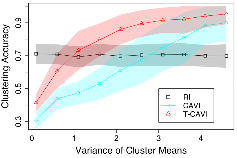
(a) $\varepsilon=0.3$

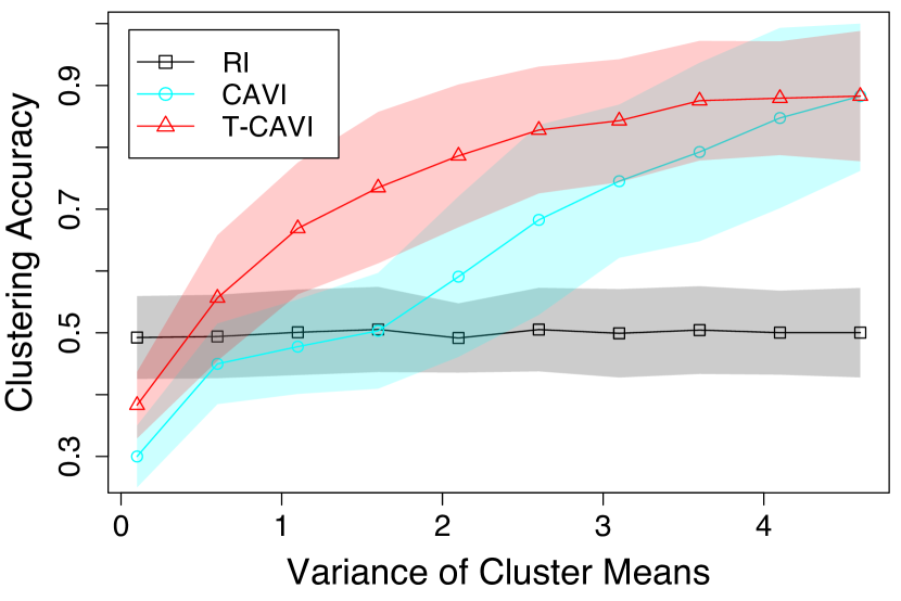
(b) $\varepsilon=0.5$

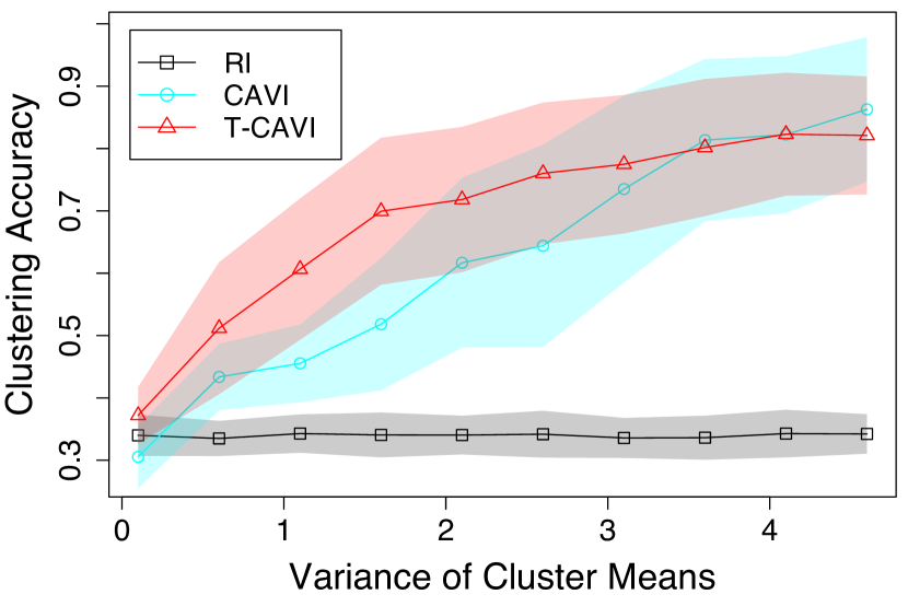
(c) $\varepsilon=0.8$

Figure 7: Performance of threshold CAVI (T-CAVI) and the classical CAVI in the Bayesian mixture of Gaussians with $n=50$, $K=5$ and $p=6$. Initializations (RI) are randomly generated from true labels with error rate $\varepsilon$.

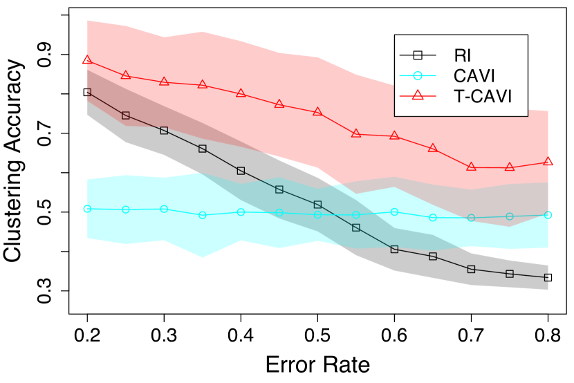
(a) $n=50$

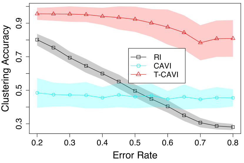
(b) $n=150$

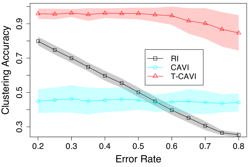
(c) $n=300$

Figure 8: Performance of threshold CAVI (T-CAVI) and the classical CAVI in the Bayesian mixture of Gaussians with $\sigma^{2}=1.5$, $K=5$ and $p=10$. Initializations (RI) are randomly generated from true labels with error rate $\varepsilon$.

Figure 9 compares the two methods under various values of data dimension $r$. Overall, T-BCAVI performs better than BCAVI, and both methods suffer when $r$ is large. This is likely due to the fact that they need to estimate a large number of parameters in that setting.

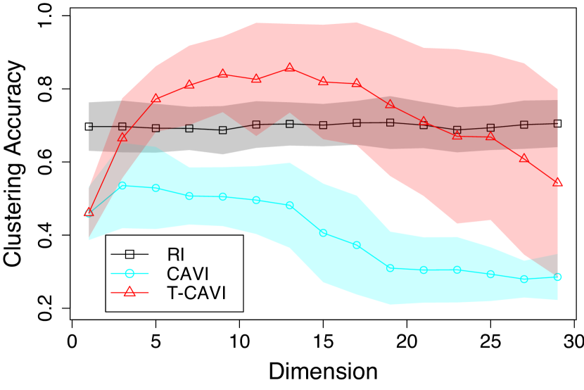
(a) $\varepsilon=0.3$

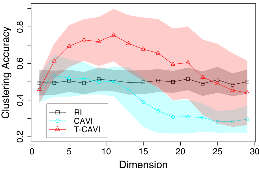
(b) $\varepsilon=0.5$

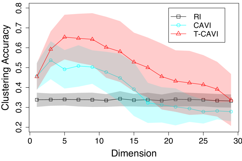
(c) $\varepsilon=0.8$

Figure 9: Performance of threshold CAVI (T-CAVI) and the classical CAVI in the Bayesian mixture of Gaussians with $n=50$, $K=5$ and $\sigma^{2}=1.5$. Initializations (RI) are randomly generated from true labels with error rate $\varepsilon$.

Figure 10 shows the behaviors of the two methods when the sample size $n$ varies. Again, T-BCAVI performs uniformly better than BCAVI, and not surprisingly, both methods become more accurate as the sample size increases.

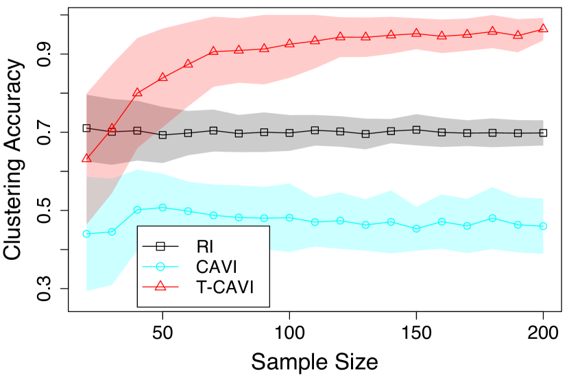
(a) $\varepsilon=0.3$

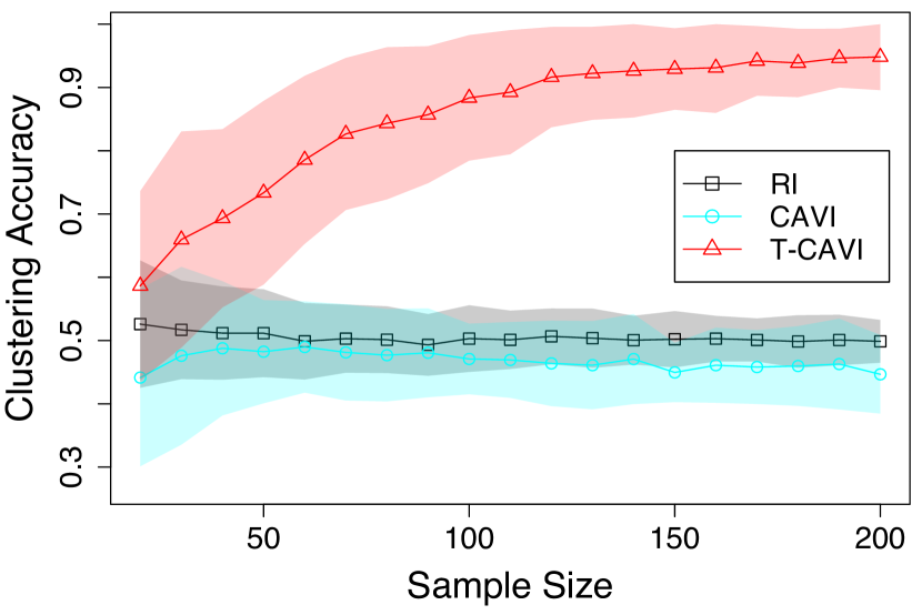
(b) $\varepsilon=0.5$

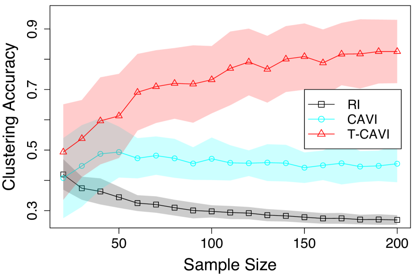
(c) $\varepsilon=0.8$

Figure 10: Performance of threshold CAVI (T-CAVI) and the classical CAVI in the Bayesian mixture of Gaussians with $\sigma^{2}=1.5$, $K=5$ and $p=10$. Initializations (RI) are randomly generated from true labels with error rate $\varepsilon$.

References

• Abbe (2018) Emmanuel Abbe. Community detection and stochastic block models: Recent developments. Journal of Machine Learning Research, 18(177):1–86, 2018.
• Adamic and Glance (2005) Lada A Adamic and Natalie Glance. The political blogosphere and the 2004 us election: divided they blog. In Proceedings of the 3rd international workshop on Link discovery, pages 36–43, 2005.
• Airoldi et al. (2008) Edoardo Maria Airoldi, David M Blei, Stephen E Fienberg, and Eric P Xing. Mixed membership stochastic blockmodels. Journal of machine learning research, 2008.
• Amini et al. (2013) Arash A Amini, Aiyou Chen, Peter J Bickel, and Elizaveta Levina. Pseudo-likelihood methods for community detection in large sparse networks. The Annals of Statistics, 41(4):2097–2122, 2013.
• Beal (2003) Matthew James Beal. Variational algorithms for approximate Bayesian inference. University of London, University College London (United Kingdom), 2003.
• Benaych-Georges et al. (2019) Florent Benaych-Georges, Charles Bordenave, and Antti Knowles. Largest eigenvalues of sparse inhomogeneous erdős–rényi graphs. The Annals of Probability, 47(3):1653–1676, 2019.
• Bickel et al. (2013) Peter Bickel, David Choi, Xiangyu Chang, and Hai Zhang. Asymptotic normality of maximum likelihood and its variational approximation for stochastic blockmodels. The Annals of Statistics, 41(4):1922–1943, 2013.
• Blei et al. (2003) David M Blei, Andrew Y Ng, and Michael I Jordan. Latent dirichlet allocation. the Journal of machine Learning research, 3:993–1022, 2003.
• Blei et al. (2017) David M Blei, Alp Kucukelbir, and Jon D McAuliffe. Variational inference: A review for statisticians. Journal of the American statistical Association, 112(518):859–877, 2017.
• Celisse et al. (2012) Alain Celisse, Jean-Jacques Daudin, and Laurent Pierre. Consistency of maximum-likelihood and variational estimators in the stochastic block model. Electronic Journal of Statistics, 6:1847–1899, 2012.
• Chin et al. (2015) Peter Chin, Anup Rao, and Van Vu. Stochastic block model and community detection in sparse graphs: A spectral algorithm with optimal rate of recovery. In Conference on Learning Theory, pages 391–423. PMLR, 2015.
• Gao et al. (2017) Chao Gao, Zongming Ma, Anderson Y Zhang, and Harrison H Zhou. Achieving optimal misclassification proportion in stochastic block models. The Journal of Machine Learning Research, 18(1):1980–2024, 2017.
• Gelfand and Smith (1990) Alan E Gelfand and Adrian FM Smith. Sampling-based approaches to calculating marginal densities. Journal of the American statistical association, 85(410):398–409, 1990.
• Grabska-Barwińska et al. (2017) Agnieszka Grabska-Barwińska, Simon Barthelmé, Jeff Beck, Zachary F Mainen, Alexandre Pouget, and Peter E Latham. A probabilistic approach to demixing odors. Nature neuroscience, 20(1):98–106, 2017.
• Holland et al. (1983) Paul W Holland, Kathryn Blackmond Laskey, and Samuel Leinhardt. Stochastic blockmodels: First steps. Social networks, 5(2):109–137, 1983.
• Jordan et al. (1999) MI Jordan, Zoubin Ghahramani, TS Jaakkola, and Lawrence K Saul. Anintroduction to variational methods for graphical models. Learning in graphical models, pages 105–161, 1999.
• Karrer and Newman (2011) Brian Karrer and Mark EJ Newman. Stochastic blockmodels and community structure in networks. Physical review E, 83(1):016107, 2011.
• Krebs (2022) Valdis Krebs. Orgnet. http://http://www.orgnet.com, 2022. [Online; accessed 18-May-2022].
• Le et al. (2017) Can M Le, Elizaveta Levina, and Roman Vershynin. Concentration and regularization of random graphs. Random Structures & Algorithms, 51(3):538–561, 2017.
• Li et al. (2020) Tianxi Li, Elizaveta Levina, and Ji Zhu. Network cross-validation by edge sampling. Biometrika, 107(2):257–276, 2020.
• Mossel et al. (2012) Elchanan Mossel, Joe Neeman, and Allan Sly. Stochastic block models and reconstruction. arXiv preprint arXiv:1202.1499, 2012.
• Newman (2013) Mark Newman. Network data. http://http://www-personal.umich.edu/%7Emejn/netdata//, 2013. [Online; accessed 18-May-2022].
• Newman (2006) Mark EJ Newman. Finding community structure in networks using the eigenvectors of matrices. Physical review E, 74(3):036104, 2006.
• Sarkar et al. (2021) Purnamrita Sarkar, YX Rachel Wang, and Soumendu Sundar Mukherjee. When random initializations help: a study of variational inference for community detection. Journal of Machine Learning Research, 22:22–1, 2021.
• Von Luxburg (2007) Ulrike Von Luxburg. A tutorial on spectral clustering. Statistics and computing, 17(4):395–416, 2007.
• Wang and Blei (2013) Chong Wang and David M Blei. Variational inference in nonconjugate models. Journal of Machine Learning Research, 14(4), 2013.
• Wang and Blei (2019) Yixin Wang and David M Blei. Frequentist consistency of variational bayes. Journal of the American Statistical Association, 114(527):1147–1161, 2019.
• Yin et al. (2020) Mingzhang Yin, YX Rachel Wang, and Purnamrita Sarkar. A theoretical case study of structured variational inference for community detection. In International Conference on Artificial Intelligence and Statistics, pages 3750–3761. PMLR, 2020.
• Zhang and Zhou (2020) Anderson Y Zhang and Harrison H Zhou. Theoretical and computational guarantees of mean field variational inference for community detection. The Annals of Statistics, 48(5):2575–2598, 2020.
• Zhang and Gao (2020) Fengshuo Zhang and Chao Gao. Convergence rates of variational posterior distributions. The Annals of Statistics, 48(4):2180–2207, 2020.