Safer Together: Machine Learning Models Trained on Shared Accident Datasets Predict Construction Injuries Better than Company-Specific Models
Submitted to Automation in Construction

Abstract

Highlights

• 9 companies from 3 domains (construction, electric T&D, oil & gas) shared their accident datasets.

• Machine learning models were trained to predict safety outcomes from fundamental attributes.

• Models trained on all datasets (full generic models) outperformed the company-specific models in 82% of the company-domain-outcome combinations, with large gains in F1 score (+4.4 on average and up to +15.3).

• On average, generic models predicted 2.26 categories more than specific models (up to 7), making for more useful forecasts in practice.

• Per-domain generic models were not always better than full generic models.

• Combining generic and specific models (data quantity and relevance) was often very beneficial.

• Generic models give companies devoid of accident datasets access to safety predictions.

• Generic models address safety cross-organizational learning and dissemination in construction.

In this study, we capitalized on a collective dataset repository of 57k accidents from 9 companies belonging to 3 domains and tested whether models trained on multiple datasets (generic models) predicted safety outcomes better than the company-specific models. We experimented with full generic models (trained on all data), per-domain generic models (construction, electric T&D, oil & gas), and with ensembles of generic and specific models. Results are very positive, with generic models outperforming the company-specific models in most cases while also generating finer-grained, hence more useful, forecasts. Successful generic models remove the needs for training company-specific models, saving a lot of time and resources, and give small companies, whose accident datasets are too limited to train their own models, access to safety outcome predictions. It may still however be advantageous to train specific models to get an extra boost in performance through ensembling with the generic models. Overall, by learning lessons from a pool of datasets whose accumulated experience far exceeds that of any single company, and making these lessons easily accessible in the form of simple forecasts, generic models tackle the holy grail of safety cross-organizational learning and dissemination in the construction industry.

1 Introduction

The SafetyAI council is a community of large organizations from the construction, oil & gas, and electric Transmission and Delivery (T&D) domains, that share their safety-related data with the SafetyAI Research and Development (R&D) team.

Before exploiting the data, the R&D team is in charge of standardizing the datasets received by each company, which is crucial, as each one features different variables and different category names for each variable. Standardization makes sure that all datasets are based on the same taxonomy, i.e., speak the same language.

The SafetyAI community dataset, comprising close to a million events including near misses, observations, good catches, etc., is only accessible to the R&D team, a neutral party, which guarantees that it is impossible for companies to see each other’s data, and that the output of all the R&D conducted on the collective dataset is made available to the entire community. This is of paramount importance, in a very competitive environment.

In this study, we started by extracting attributes from accident reports. We briefly introduce the attribute framework in what follows.

1.1 Attribute-based framework

Attributes are basic descriptors of construction work that are observable before accident occurrence, and cover means, methods, and environmental conditions [1, 2]. One advantage of the attribute-based framework over modeling at the task or work package level is that attributes are fundamental and universal. That is, any situation from any site around the world, in any industry sector, can be characterized by a set of attributes. Attributes can be recorded on-the-fly on site, or can be extracted offline from various mediums such as photos and text reports. For instance, four attributes can be extracted from the narrative worker tripped on a cable when carrying a 2x4 to his truck: (1) cable, (2) object on the floor, (3) lumber, and (4) light vehicle.

Narratives are particularly well-suited if the goal is to use attributes for predictive modeling. Indeed, in incident report databases, narratives are often paired with outcomes such as accident type, injury severity, body part impacted, etc. Attributes also completely anonymize narratives, which is especially desirable when considering a pool of datasets aggregated from different companies. For any given event, everything that remains is a set of attributes and a set of standardized safety outcomes.

However, manually extracting attributes from large amounts of text reports is very costly in terms of human resources and pose inter-annotator agreement issues. To solve this problem, we developed and validated a Natural Language Processing (NLP) tool based on rules and lexicons [3]. We later proved that using the attributes extracted by the tool to predict safety outcomes was effective and valid [4, 5]. We also used the attributes extracted by the tool for unsupervised learning applications, such as clustering and visualization [6], and risk modeling and simulation [7].

1.2 Differences with our previous research and objective of the current study

In our original study [4], we provided a proof for the concept of predicting safety outcomes from attributes, both extracted with the NLP tool. Then, in [5], we showed that attributes were still highly predictive when the safety outcomes were given by independent human annotations, which definitely validated the approach. We also used a much larger dataset than in the original study, two new supervised learning algorithms, model stacking, a healthier experimental setup with more appropriate performance metrics, and we analyzed per-category attribute importance scores. We also showed that unlike what we had concluded in [4], injury severity was predictable from attributes.

In the present research, we interested ourselves with a new, completely different problem. We had access to a pool of accident datasets coming from 9 companies, and our goal was to:

“Test whether predictive models trained on a generic dataset (i.e., aggregated from the datasets of multiple companies) outperformed the models trained on the specific dataset of each company.”

More precisely, we experimented with two types of generic models:

• Full generic model: one model trained on the datasets of all companies.

• Per-domain generic models: one model per industry sector, trained only on the datasets of the companies involved in that sector (or the parts thereof, as some companies belong to multiple domains).

The potential advantages of generic models are numerous:

1. Usually with machine learning, the more data, the better, so generic models are expected to bring improvements in predictive skill compared to the company-specific models. This is not guaranteed however, as one important question is whether (1) more data (generic datasets) or (2) more relevant data (specific datasets) is better.

2. By being trained on larger datasets, the generic models learn to predict a greater variety of outcome categories than the specific models, making for more useful forecasts.

3. Successful generic models would remove the needs for training specific models for each company, saving a lot of time and resources.

4. Alternatively, if company-specific models are already available, combining them with the generic models may provide an extra boost in performance.

5. Last but not least, successful generic models would give small companies -whose accident datasets are too limited to train their own specific models- access to high quality safety outcome forecasts.

From a high level, generic models tackle the holy grail of safety cross-organizational learning and dissemination in the construction industry. Indeed, generic models (1) learn lessons from a pool of datasets whose quantity and diversity of accumulated experience far exceeds that of any single company, and (2) disseminate these lessons as forecasts, which are clear, direct, and easily accessible information, via, e.g., a user interface (desktop or mobile) or API taking attributes as input and returning probabilities for each category of each outcome.

Moreover, one should note that in the pool, the individual biases of each dataset, due to specific annotators, reporting practices and policies, etc., tend to average out. Consequently, the lessons learned by the supervised learning algorithms on the generic datasets are more objective and broadly applicable than that learned on the specific datasets.

2 Background

The needs to share standardized incident data at the industry level to enable collaborative learning have long been recognized in aviation and transportation [8]. Some examples include the NASA-managed Aviation Safety Reporting System (ASRS) database, created in 1976 and featuring over a million incidents, or the European Coordination Center for Accident and Incident Reporting Systems (ECCAIRS) database, started in 2004. Such collective repositories also exist in the chemical industry, with the Major Accident Reporting System (eMARS) of the European Commission, launched in 1982, and the Process Safety Incident Database (PSID) of the Center for Chemical Process Safety [9].

However, the construction industry still lacks comparable initiatives. The needs for data storage and access infrastructures for construction safety did start to receive some attention recently [10, 11], but most efforts placed themselves at the company or project level. Cross-organizational safety data collection is still rare in practice [12, 13]. This is a major issue, as collaborative machine learning at the industry level is not possible until a common pool of standardized datasets has been put together. This provided the motivation for us to create the SafetyAI council in 2020.

One should note that some consortiums already exist, such as the INGAA Foundation, the Edison Electric Institute (EEI), the Construction Safety Research Alliance (CSRA), or the National Safety Council (NSC), but their activities do not revolve around systematic large-scale accident data collection and analysis. These initiatives rather involve working groups, communities of practice, qualitative analyses, and conferences, towards building communications, policies, best practices, business intelligence, safety culture and leadership, training material, etc. In other words, they are based on “soft” methods for knowledge sharing and collaborative learning at the human level. They do not primarily conduct “hard” scientific research and software development, and do not pool accident datasets for AI applications and automatic large-scale learning and dissemination.

3 Data Description

As already explained, as part of the SafetyAI initiative, we had access to a pool of safety datasets coming from nine large companies from the construction, oil & gas, and electric Transmission and Delivery (T&D) domains. One company, Company7, also had about 600 corporate services (office) events for the severity outcome. We kept these cases as training data for the full generic model but did not train a specific model on them.

Member companies conduct work mostly in North America, and rely on their own teams as well as contractors. The collective dataset covers the period 2000 to 2022, with a distribution biased towards the last decade and especially more recent years.

While the entire pool comprises almost a million events including near misses and observations, we focused on accident cases only in this effort. As can be seen in Table 1, the sizes of the individual datasets ranged from 2k to 20k cases, with an average of 6k per company. There were 57262 accident cases in total, recorded over tens of millions of work hours.

	Comp.1	Comp.2	Comp.3	Comp.4	Comp.5	Comp.6	Comp.7	Comp.8	Comp.9
Domains	Constr., elec.	Oilgas	Constr., oilgas	Elec.	Constr.	Constr., elec.	Elec., oilgas, corp.	Oilgas	Elec.
Regions	Canada	California	NAM	NAM	NAM	NAM	NAM, Mexico	World⋆	Southeast USA
$n$	4481	1965	4072	5321	7245	4310	8345	19298	2225

Table 1: Company overview. NAM: North America (Canada + USA). Constr.: construction. Elec: electric T&D. Oilgas: oil & gas. ^⋆Including ships and rigs. Corp: corporate.

We considered the same outcomes as in [5]: injury severity, body part impacted, injury type, and accident type. The columns corresponding to each outcome were selected from the company datasets and normalized to use a common, standard set of categories, shown in Table 2. Not all outcomes were available for every event of every company. From the narrative of each report, we extracted with the NLP tool [3] the original set of 80 attributes [3, 5], plus 11 new items (see Table 7). We also used the tool to extract a fifth outcome, energy source, that was not available in the company datasets.

Injury Severity		Body Part		Injury Type		Accident Type		Energy Source
first aid	38994	hand	15782	cut	14086	handling	6379	motion	33958
report-only	6993	head	10296	strain	10069	fall	5374	gravity	15904
lost time	5319	leg	6550	contusion	8558	exposure	3986	chemical	2411
medical	4913	arm	5943	foreign body	3348	struck	3834	biological	2044
recordable	1043	trunk	5375	pinch	1756	contact	2269	thermal	1691
		foot	4632	fracture	1681	caught	1758	mechanical	611
		multiple/entire	942	burn	1454	overexertion	1523	pressure	296
				irritation	1222	equipment	1449	electricity	181
				pain	1194	PPE	949	radiation	166
				exhaustion	1054	transitioning	578
				bite	710	error	425

Table 2: Outcome category counts, across all companies and domains. PPE: personal protective equipment.

4 Experimental Setup

4.1 Splits

Train, validation and test splits were created for each of the 51 company-domain-outcome combinations for which at least 2 categories with more than 100 observations each were available (shown in Table 4), by randomly sampling without replacement 64%, 16%, and 20% of cases, respectively. The counts summed over companies are shown in Table 3. Note that the proportions we used in our previous work [5] were 81%, 9% and 10%, but in the present research, we decided to reserve more observations for the validation and test sets to make them more representative of the training sets, in order to increase the stability and validity of hyperparameter tuning and evaluation.

		# Companies	Train	Val	Test
Severity	Construction	4	9980	2494	3119
	Electric T&D	4	6672	1669	2085
	Oil & Gas	4	18381	4595	5744
	Corporate	1	418	105	131
	Full	9	35451	8863	11079
Body Part	Construction	4	8209	2052	2565
	Electric T&D	4	6036	1508	1885
	Oil & Gas	3	15788	3947	4933
	Full	9	30033	7507	9383
Injury Type	Construction	4	6267	1566	1958
	Electric T&D	4	4764	1191	1489
	Oil & Gas	3	14960	3740	4675
	Full	9	25991	6497	8122
Acc. Type	Construction	2	2740	685	856
	Electric T&D	2	1600	400	500
	Oil & Gas	3	2910	728	910
	Full	6	7250	1813	2266
En. Source	Construction	4	4875	1218	1524
	Electric T&D	3	2637	660	825
	Oil & Gas	2	2600	650	813
	Full	8	10112	2528	3162

Table 3: Split counts for each domain-outcome combination, summed over companies. For # Companies, full $\neq$ total as some companies belong to multiple domains (see Tables 1 and 4).

A specific model was trained on each of the 51 company-domain-outcome combinations for which sufficient data were available, except for that one combination involving the corporate cases, making for a total of 50 specific models.

Construction

Electric T&D

Oil & Gas

Corp.

Comp.

S

B

IT

AT

E

S

B

IT

AT

E

S

B

IT

AT

E

S

1

x

x

x

x

2

x

x

x

3

x

x

x

x

x

x

x

4

x

x

x

x

x

5

x

x

x

x

x

6

x

x

x

x

x

x

x

x

7

x

x

x

x

x

x

x

x

x

8

x

x

x

x

x

9

x

x

x

x

x

Table 4: The 51 company-domain-outcome combinations associated with at least 2 categories with more than 100 observations each. S: severity, B: body part, IT: injury type, AT: accident type, E: energy source. Corp.: corportate.

For a given domain and a given outcome, the splits of the per-domain generic model were obtained by combining, across all companies, the splits corresponding to that domain and that outcome. In total, there was one per-domain generic model for each domain and for each outcome, hence a total of $3\times 5=15$ per-domain generic models.

For a given outcome, the splits of the full generic model were obtained by combining, across all companies and across all domains, the splits corresponding to that outcome. In total, there was one full generic model for each outcome, hence a total of 5 full generic models.

For each of the aforementioned cases, we tried 3 different algorithms, as will be explained in subsection 4.3. Hence, a total of $(15+5)\times 3=60$ generic models were trained.

4.2 Class imbalance

To address the problem of class imbalance, weights inversely proportional to category counts in the training set were computed with the formula max(counts)/counts, like in [5]. During training, these weights forced the models to pay more attention to the cases from the minority categories. Per-category counts with training weights can be found in Tables 8 and 9 for the 15 domain-outcome combinations.

4.3 Supervised learning algorithms

Like in [5], we relied on three popular machine learning models: Random Forest (RF) [14], eXtreme Gradient Boosting (XGBoost or XGB) [15], and linear Support Vector Machine (SVM) [16]. More precisely, we used the Python’s scikit-learn implementations of Random Forest and linear SVM, while, for XGBoost, we used the original Python library and in particular the GPU-accelerated implementation of the “fast histogram” algorithm (gpu_hist) as the tree method.

For theoretical details about each algorithm, we refer the reader to our paper [5], publicly available.

4.4 Hyperparameter optimization

We tuned the models by performing grid searches on the validation sets. Details about the parameters searched are available in C. The final models were trained on the union of the training and validation sets with the best parameter values. Both the specific models and the generic models were tested on the test sets of the specific models, to ensure fair comparison. As already explained, there were 50 such test sets, one for each company-domain-outcome combination.

4.5 Transfer learning by stacking generic and specific models

As was mentioned in the introduction, one important question is the extent to which (1) more data (generic datasets) or (2) more relevant data (specific datasets) is better. In what follows, we explore a way to move past this binary choice and have a tradeoff between quantity and relevance.

Inspired by transfer learning, which is very successful in computer vision [17] and NLP [18, 19, 20, 21], we experimented with combining the predictions of the generic and specific models via an ensemble model.

Very briefly, in AI, transfer learning refers to a two-step process. First, a model is trained at solving a general task on large amounts of data. This phase is called the pretraining phase, as it allows the model to acquire generic knowledge (e.g., in NLP, reading and writing), that is applicable to a great variety of situations downstream. Second, the pretrained model is finetuned on a specific task of interest, often associated with a much smaller dataset (e.g. in NLP, summarization, classification, question answering, paraphrase detection, etc.).

In our case, the generic and the specific models have to perform the same task, i.e., predicting a given safety outcome, and there is no pretraining phase per se, in that the generic and the specific models are two different models. However, our approach is similar in spirit to transfer learning, as our goal is to capitalize on generic knowledge gained from large amounts of data to improve performance on a specific task associated with a smaller dataset.

More precisely, for each company-domain-outcome combination, we trained a meta-model taking as input the weighted elementwise sum of the probabilistic forecasts of the best generic and specific models. We used a simple logistic regression as our meta-model, with the $C$ parameter fixed and equal to $0.2$, like in [5]. We grid searched the validation set to find the best values of coefficients $a$ and $b$ where:

$$\text{input}_{\text{ensemble}}=a\times\text{output}_{\text{generic}}+b\times\text{output}_{\text{specific}}$$ (1)

Besides performance considerations, using tunable weights improves interpretability, by providing information regarding which of the generic model or the specific model makes the most important contribution to predictive skill.

We tried values from $0.1$ to $1$ with $0.1$ steps, holding the other parameter equal to $1$, and conversely. That is, the following 19 pairs: $(0.1,1)$, $(0.2,1)$, … , $(1,1)$, $(1,0.1)$, $(1,0.2)$, … , $(1,0.9)$.

SVM issue. By design, the implementation of the linear SVM model we used, linearSVC, only returns discrete predictions, that is, a single label corresponding to the most likely category, rather than a probability distribution over all categories. To address this issue, in [5], we tried retraining the best SVM using the SVC implementation with linear Kernel. However, results were not convincing. Therefore, in the present study, we decided simply not to use model stacking when one of the two models involved (e.g., best generic or specific model) was a SVM.

4.6 Performance metrics

Due to the large class imbalance for all outcomes, measuring classification performance with accuracy was inadequate. Rather, we computed precision, recall, and F1-score.

Precision, respectively recall, for category $i$, is equal to the number of correct predictions for category $i$ (number of hits), divided by the number of predictions made for category $i$ (hits and false alarms), respectively by the number of observations in category $i$ (hits and misses).

$$\textrm{precision}=\frac{C_{i,i}}{\sum_{j=1}^{K}C_{j,i}}\hskip 56.9055pt\textrm{recall}=\frac{C_{i,i}}{\sum_{j=1}^{K}C_{i,j}}$$ (2)

Where the confusion matrix $C$ is a square matrix of dimension $K\times K$ ($K$ being the number of categories) and whose $(i,j)^{th}$ element $C_{i,j}$ indicates how many of the observations known to be in category $i$ were predicted to be in category $j$. Finally, we computed the F1-score, the harmonic mean of precision and recall:

$$\text{F1}=2\times\frac{\text{precision}\times\text{recall}}{\text{precision}+\text{recall}}$$ (3)

4.7 Configuration

We relied on a single Ubuntu 20.04.4 machine featuring a 4.9 MHz 12-thread CPU, a 12 GB Nvidia Titan V GPU, 64 GB of RAM, R version 4.1.3 [22], and Python version 3.8.13 with scikit-learn version 1.1.1 [23]. Running all experiments took approximately ten days.

5 Results

Each generic model (full and per-domain), as well as ensembles thereof (stacking approach described in section 4.5) was tested on the test set of each company-domain-outcome combination and compared against the best performing specific model for this combination.

Results are very positive. As can be seen in Table 5, across all companies, the generic models (full or per-domain) outperform the specific models 82% of the time, i.e., for 41 company-domain-outcome combinations out of 50. Detailed per-company results can be found in E for the full generic models and F for the per-domain generic models. At the company level, improvements are brought on average for 80.6% of outcomes (across all domains), ranging from 33.3% for Company2 to 100% for Company1, Company4, Company6, and Company9.

	Construction					Electric T&D					Oil & Gas
C	S	B	IT	AT	E	S	B	IT	AT	E	S	B	IT	AT	E
1	+1.26	+0.2	+2.55		+3.07
2											x	+3.15	x
3	x	+6.56	+0.49	x	+12.47						+0.99			x
4						+3.49	+0.47	+3.06	+0.98	+0.63
5	x	+2.64	+1.29	+3.14	+2.79
6	+12.86	+4.39	+1.63		+7.09	+12.87	+5	+11.19		+0.59
7						x	+6.69	+15.3			x	+1.04	+9.54	+2.12	+2.2
8											+1.11	+0.47	+2.78	x	+3.13
9						+1.56	+5.38	+12.16	+5.01	+6.16

Table 5: Company-level max gains. x: no improvement. S: severity, B: body part, IT: injury type, AT: accident type, E: energy source. C: company

Furthermore, as shown in Fig. 1, gains are high on average (+4.4 in F1 score) and reach impressive values, e.g., +15.3 for Company7 on electric T&D-injury type, +12.87 for Company6 on electric T&D-severity, +12.86 for Company6 on construction-severity, +6.56 for Company3 on construction-body part, etc. And all of that, while predicting more categories.

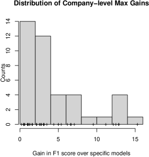
Figure 1: Company-level max gains, across all domains and outcomes. n=41, min=0.2, max=15.3, mean=4.4.

There are only 9 domain-outcome combinations over 50, across 5 companies, on which the generic models do not bring any quantitative improvement. However, since their forecasts are more informative (more categories predicted), it may still make sense in practice to use the generic models in lieu of the specific models, even on these combinations. For instance, for Company3-oil & gas-accident type, the specific model only predicts exposure and struck, but the generic model also predicts the categories caught, fall, and overexertion.

The F1 scores averaged over all companies are shown in Table 6. Overall, the generic models bring improvement over the specific models for 73.3 % of the domain-outcome combinations (11 out of 15). As shown on the right of Fig. 2, maximum gains range from 0.95 (for electric T&D-energy source) to 9.98 (for electric T&D-injury type) with an average of 3.37. Also, not only do the 11 best generic models outperform their specific counterparts with a comfortable margin, but they also generate finer-grained forecasts, which are much more useful in practice.

More specifically, generic models predict 2.26 additional categories on average, even up to 7 for construction-injury type (while still providing a gain of 3.48 in F1 score). This is remarkable, considering that the more categories to be predicted, the more difficult the task (see D).

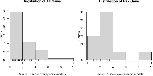
Figure 2: Gains averaged over companies. Left: n=48, min=0.16, max=9.98, mean=2.22. Right: n=11, min=0.95, max=9.98, mean=3.37.

The construction and oil & gas domains see gains for 3 outcomes out of 5, while on the electric T&D domain, we observe improvement for every outcome. Further, for the body part, injury type, and energy source outcomes, there is at least one generic model that outperforms its specific counterpart, on every domain, while the severity and accident type outcomes see improvements only on the electric T&D domain.

However, it is important to note that even on those 4 domain-outcome combinations on which the generic models do not offer gains in predictive performance, it can still be desirable to use them in practice over the specific models, as they generate more informative forecasts, with 2 additional categories predicted, on average.

Overall, more than half of all F1 scores recorded for the generic models (79 out of 150, or 53%) are greater or within two points of that of the specific models, while predicting 1.83 more categories on average. And, as shown on the left of Fig. 2, the 48 generic models that outperform their specific counterparts bring on average an improvement of 2.22 in F1 score.

5.1 Body part, injury type, and energy source

Some of the greatest improvements are observed for injury type, where the best generic models provide large average gains of 3.48, 9.98, and 3.07, respectively on the construction, electric T&D, and oil & gas domains, while predicting on average 4.25 more categories than the company-specific models. This large boost in performance is remarkable considering the significant increase in task difficulty.

Similarly, for energy source, the best generic models provide 4.48, 0.95, and 1.83 improvements in F1 score, while predicting 1.53 more categories on average; and for body part, the gains are 3.38, 3.42, and 1.37, with 0.17 more categories predicted.

5.2 Severity and accident type

For severity and accident type, the generic models outperform the company-specific ones on the electric T&D domain, with 3.09 and 2.03 gains in F1 scores, while predicting 2 and 0.5 more categories on average.

On the construction and oil & gas domains, the best generic models are between 2.4 and 6 points below the company-specific ones. However, they still offer the benefit of predicting more categories (+1.6 on average).

				Construction		Electric T&D		Oil & Gas
				Full	Dom.	Full	Dom.	Full	Dom.
Severity	F1	SVM	gen	31.66	30.29	35.52	35.79	30.92	28.97
		RF	gen	27.26	31.04	33.37	41.28	23.48	26.08
			ens	30.33	31.82	41.17†	43.88†	28.98	30.76
		XGB	gen	26.98	28.74	36.4	39.69⋆	24.25	24.19
			ens	29.67	31.81	40.01⋆	40.95	29.14	31.44
			spec	35.34†		40.79		33.86†
	Count	# categories	spec	3.5		3		3.5
			gen	5	5	5	5	5	5
		# datasets		9	4	9	4	9	4
Body Part	F1	SVM	gen	25.51	31.32	26.68	25.24	23.65	24.66
		RF	gen	34.41†	31.81	34.94†	33.05	30.22†	28.85†
			ens	30.33⋆	30.39⋆	34.08	29.25	26.43	27.54⋆
		XGB	gen	32.86	32.23†	33.76	35.21†	29.22	28.59⋆
			ens	29.05⋆	29.2⋆	32.31	34.71	26.37	27.74⋆
			spec	31.03		31.79		28.85
	Count	# categories	spec	6		5.5		6
			gen	6	6	6	6	6	6
		# datasets		9	4	9	4	9	3
Injury Type	F1	SVM	gen	38.73	42.78⋆	53.7†	42.91⋆	35.11⋆	33.89
		RF	gen	40.03	42.11⋆	42.44⋆	41.68⋆	32.15	32.82
			ens	41.75	45.46†	49.42	45.10	38.65†	38.97
		XGB	gen	36.76	42.55⋆	41.03	41.48	31.33	32.34
			ens	47.4†	45.45	51.44	49.28†	38.05	39.79†
			spec	43.92		43.72		36.72
	Count	# categories	spec	4		5.25		7
			gen	11	6	11	8	11	11
		# datasets		9	4	9	4	9	3
Accident Type	F1	SVM	gen	42.39	42.20	44.58	44.84	60.69	64.85
		RF	gen	42.46	42.42	48.58†	50.2†	63.14	64.12
			ens	44.35	40.8	41.29	39.72	66.40	65.74
		XGB	gen	48.27	49.21	47.80⋆	49.58	58.58	63.04
			ens	42.02	43.40	41.08	43.53	64.56	67.13
			spec	54.98†		48.17		73.16†
	Count	# categories	spec	3.5		4.5		2.67
			gen	5	5	5	5	5	4
		# datasets		6	2	6	2	6	3
Energy Source	F1	SVM	gen	74.12†	73.78	77.64⋆	78.87†	69.54⋆	55.63
		RF	gen	72.71	73.91†	77.12⋆	78.61	71.12	70.72†
			ens	69.06⋆	69.64⋆	75.83	76.48⋆	70.58	69.12⋆
		XGB	gen	73.77	71.04	78.83†	75.61	72.22†	70.35⋆
			ens	69.05⋆	70.23	76.47⋆	75.03	70.98	70.38⋆
			spec	69.64		77.92		70.39
	Count	# categories	spec	2.25		2.67		3
			gen	5	3	5	3	5	4
		# datasets		8	4	8	3	8	2

Table 6: Results averaged over companies. $\dagger$: best of their sub-column. Bold/$\star$: better than/within 2 pts of spec. Full: full generic model (one per outcome, same across domains). Dom.: per-domain generic model (one per outcome per domain). Gen/spec: generic/specific. Ens: ensemble thereof. # datasets: number of company datasets forming the generic dataset. Note: for the same outcome, # categories and # datasets are the same for Full across domains, we repeat them only to ease comparison.

5.3 Full vs. per-domain

In what follows, we refer to the full and per-domain models and their ensemble versions. When considering full generic models, the average improvement in F1-score over the specific models is 2.85 and there are 2.44 additional categories predicted (min=0, max=7), while when considering per-domain generic models, the average improvement is 2.57 and 1.38 additional categories are predicted (min=0, max=4). The per-domain models reach a higher max score than the full models on 9 combinations out of 15 (60%), and in 5 out of 11 (45%) when the specific models are outperformed. The full and per-domain models outperform the specific models on the same 11 domain-outcome combinations.

So, in terms of performance, there is no clear winner. However, since the full generic models predict more categories, and are also simpler conceptually (just one model per outcome), full models seem like the way to go. This conclusion however will need to be validated when more datasets are available for each domain. One thing to note, however, is that specific models may still be desirable in the context of model stacking, as covered next.

5.4 Generic vs. ensemble (generic + specific)

The transfer learning-like stacking approach, i.e., combining the predictions of the generic and specific models, boosts performance over the generic models (both full and per-domain) on all domains for the severity and injury type outcomes, in some cases for accident type, and nowhere for body part and energy source.

For severity, the average gains are of 3.93, and range from 0.78 to an impressive 7.8 (for electric T&D-full-RF). Results are even more impressive for injury type. Gains range from 1.72 to 10.64 (for construction-full-XGB), with a high average of 6.17.

It is interesting to note that for severity and injury type, very few of the generic models outperform the specific models in the first place, and it is only by combining their predictions with that of the specific models that absolute best performance can be reached, on the electrical domain for severity, and on all domains for injury type.

We also observe that conversely, for body part and energy source, where model stacking does not bring additional skill, the generic models are stronger than the specific models in the first place.

All in all, these results may suggest that ensembling only works when the generic models are not already better than the specific models. However, this rule does not hold everywhere (e.g., construction-accident type-XGB), so additional data, experiments and results will be necessary to draw any general conclusion here.

5.5 Quantity vs. relevance

As far as whether more data or more relevant data is best, Fig. 3 shows the distributions of the best $a$ and $b$ coefficients as determined on the validation sets. It tends to indicate that, on average, the best tradeoff involves anywhere from a little bit to a lot of generic model (anywhere in the [0.1,1] range, with peaks towards [0.1,0.2] and [0.9,1]), but almost always a lot of specific model (between 0.9 and 1). In other words, data relevance always seems important, while the contribution of data quantity fluctuates. However, this is only a general trend. As can be seen in the detailed results per company (E and F), in some cases, the contribution of the generic model is more important than that of the specific model, e.g., (1,0.6) for Company6-XGB in the first table of F.

5.6 Best model type

For the full generic models, the best algorithm is RF (6 domain-outcome combinations over 15), followed by SVM (5/15) and XGB (4/15). When stacked with the specific model, RF reaches best performance in 10 out of 15 combinations.

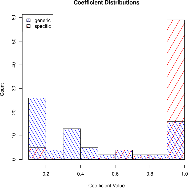
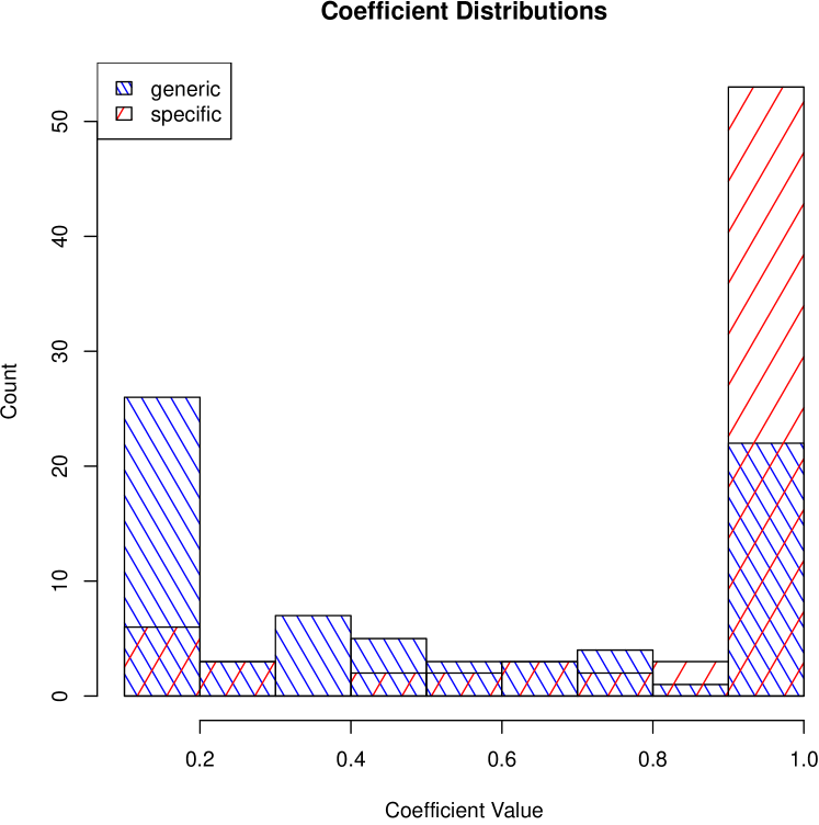
Figure 3: Distributions of the best coefficient values $a$ (generic) and $b$ (specific). Left: full. Right: per-domain.

When considering the per-domain generic models, SVM obtains the best score 7 times out of 15, followed by RF (5/15) and XGB (3/5). However, when used in the ensemble, XGB is the best (10/15).

RF and XGB are better choices than SVM as they consistently top the scores and can be used in ensembles. In terms of performance though, there is no clear winner between the two. One or the other could be used interchangeably. However, XGBoost is superior in practice as far as deployment is concerned, as the Random Forest models take a lot of disk space, even after applying some compression tricks.

6 Conclusion

We showed that generic models provide consistent and large improvements over company-specific models. Moreover, generic models issue finer-grained forecasts that are more useful in practice, as they predict more categories of each safety outcome.

Generic models remove the needs for training company-specific models, saving a lot of time and resources, and give small companies, whose accident datasets are too limited to train their own models, access to safety outcome predictions.

Per-domain generic models (trained on data from a specific industry sector) are not always better than full generic models (trained on all data). Ensembling generic and specific models is often very beneficial. Therefore, it might still be worth training specific models to combine their predictions with that of the generic models. If specific models are already in use, combining them with the generic models may provide a boost in performance.

The forecasts are in essence clear and direct information that can be accessed via a user interface (as a desktop or mobile webpage or application), or via an API for integration into any existing ecosystem. In each case, the only input required is a set of attributes, and the output are probabilities for each category of each outcome.

By learning lessons from a pool of datasets whose accumulated experience far exceeds that of any single company, and making these lessons easily accessible, generic models tackle the holy grail of safety cross-organizational learning and dissemination in the construction industry.

7 Acknowledgements

We thank the Nvidia corporation for donating the Titan V GPU that was used in this research, as part of their GPU grant program.

8 References

Appendices

Appendix A Attribute List

adverse low temps	fuses⋆	machinery	spark
bolt	grinding	manlift	splinter/sliver
breaker⋆	grout	mud	spool
cable	guardrail/handrail	nail	stairs
cable tray	hammer	no/improper PPE	steel/steel sections
chipping	hand size pieces	object at height	stripping
cleaning	hazardous substance	object on the floor	stud
clearance⋆	heat source/high temps	piping	switch/switching⋆
concrete	heater⋆	pole⋆	tank
concrete liquid	heavy material/tool	pontoon	transformer⋆
conduit	heavy vehicle	poor housekeeping	uneven surface
confined work space	hose	poor visibility	unpowered tool
congested work space	improper body position	powered tool	unpowered transporter
crane	improper procedure/inattention	rebar	unstable support/surface
door	improper security of materials	relay⋆	valve
drill	improper security of tools	repetitive motion	vault⋆
dunnage	insect/animal	scaffold	welding
electricity	job trailer	screw	wind
exiting	ladder	sharp edge	wire
fan⋆	lifting/pulling/manipulating	slag	working at height
fatigued dizzy	light vehicle	slippery surface	working below elev wksp/mat
forklift	LOTO/labeling⋆	small particle	working overhead
formwork	lumber	soffit	wrench

Table 7: 92 attributes used in this study. LOTO: lockout-tagout. PPE: personal protective equipment. $\star$: eleven new attributes added since [4, 5].

Appendix B Detailed split counts

Severity
		Train	$w$	Val	Test
Construction	report-only	917	8.2	226	283
	1st aid	7486	1.0	1876	2369
	medical	470	15.9	114	140
	recordable	147	50.9	28	42
	lost time	960	7.8	250	285
	total	9980		2494	3119
Electric T&D	report-only	2392	1.2	576	712
	1st aid	2809	1.0	736	905
	medical	554	5.1	140	162
	recordable	310	9.1	74	101
	lost time	607	4.6	143	205
	total	6672		1669	2085
Oil & Gas	report-only	929	14.8	244	279
	1st aid	13766	1.0	3405	4279
	medical	1919	7.2	489	618
	recordable	152	90.6	42	52
	lost time	1615	8.5	415	516
	total	18381		4595	5744
Corporate	report-only	97	3.3	31	22
	1st aid	321	1.0	74	109
	total	418		105	131
Full	report-only	4335	5.6	1077	1296
	1st aid	24382	1.0	6091	7662
	medical	2943	8.3	743	920
	recordable	609	40.0	144	195
	lost time	3182	7.7	808	1006
	total	35451		8863	11079

Body Part
		Train	$w$	Val	Test
Construction	arm	1059	2.6	285	338
	foot	694	3.9	167	232
	hand	2732	1.0	701	864
	head	1682	1.6	394	494
	leg	958	2.9	262	307
	trunk	1084	2.5	243	330
	total	8209		2052	2565
Electric T&D	arm	1061	1.4	274	319
	foot	372	4.0	89	135
	hand	1473	1.0	368	452
	head	1246	1.2	318	403
	leg	1084	1.4	251	307
	trunk	800	1.8	208	269
	total	6036		1508	1885
Oil & Gas	arm	1445	3.9	386	477
	foot	1741	3.2	421	568
	hand	5586	1.0	1385	1740
	head	3514	1.6	887	1088
	leg	2053	2.7	498	596
	trunk	1449	3.9	370	464
	total	15788		3947	4933
Full	arm	3565	2.7	945	1134
	foot	2807	3.5	677	935
	hand	9791	1.0	2454	3056
	head	6442	1.5	1599	1985
	leg	4095	2.4	1011	1210
	trunk	3333	2.9	821	1063
	total	30033		7507	9383

Accident Type
		Train	$w$	Val	Test
Construction	caught	396	2.3	105	137
	exposure	119	7.8	38	40
	fall	803	1.2	200	243
	overexertion	492	1.9	128	160
	struck	930	1.0	214	276
	total	2740		685	856
Electric T&D	caught	207	2.2	55	62
	exposure	454	1.0	123	142
	fall	403	1.1	102	143
	overexertion	288	1.6	51	65
	struck	248	1.8	69	88
	total	1600		400	500
Oil & Gas	caught	198	7.7	43	53
	exposure	526	2.9	127	184
	fall	1527	1.0	393	463
	struck	659	2.3	165	210
	total	2910		728	910
Full	caught	801	3.4	203	252
	exposure	1099	2.5	288	366
	fall	2733	1.0	695	849
	overexertion	780	3.5	179	225
	struck	1837	1.5	448	574
	total	7250		1813	2266

Energy Source
		Train	$w$	Val	Test
Construction	chemical	76	42.7	21	14
	gravity	1551	2.1	405	479
	motion	3248	1.0	792	1031
	total	4875		1218	1524
Electric	biological	221	7.6	52	88
	gravity	733	2.3	179	230
	motion	1683	1.0	429	507
	total	2637		660	825
Oil & Gas	chemical	70	21.2	13	21
	gravity	1485	1.0	361	448
	motion	914	1.6	246	300
	thermal	131	11.3	30	44
	total	2600		650	813
Full	biological	221	26.4	52	88
	chemical	146	40.0	34	35
	gravity	3769	1.6	945	1157
	motion	5845	1.0	1467	1838
	thermal	131	44.6	30	44
	total	10112		2528	3162

Table 8: Split counts (1/2). $w$: training weights.

Injury Type
		Train	$w$	Val	Test
Construction	contusion	728	3.6	185	229
	cut	2644	1.0	682	795
	fob	399	6.6	84	118
	fracture	100	26.4	24	39
	pinch	267	9.9	90	97
	strain	2129	1.2	501	680
	total	6267		1566	1958
Electric T&D	bite	129	12.3	35	42
	burn	75	21.2	14	21
	contusion	861	1.8	216	277
	cut	1305	1.2	330	400
	fob	209	7.6	46	69
	fracture	176	9.0	39	53
	irritation	420	3.8	101	141
	strain	1589	1.0	410	486
	total	4764		1191	1489
Oil & Gas	bite	168	27.6	39	52
	burn	572	8.1	150	179
	contusion	3587	1.30	848	1091
	cut	4638	1.0	1160	1509
	exhaustion	75	61.8	24	25
	fob	1440	3.2	381	455
	fracture	622	7.5	160	199
	irritation	127	36.5	37	42
	pain	704	6.6	176	215
	pinch	720	6.4	181	231
	strain	2307	2.0	584	677
	total	14960		3740	4675
Full	bite	297	28.9	74	94
	burn	647	13.3	164	200
	contusion	5176	1.7	1249	1597
	cut	8587	1.0	2172	2704
	exhaustion	75	114.5	24	25
	fob	2048	4.2	511	642
	fracture	898	9.6	223	291
	irritation	547	15.7	138	183
	pain	704	12.2	176	215
	pinch	987	8.7	271	328
	strain	6025	1.4	1495	1843
	total	25991		6497	8122

Table 9: Split counts (2/2). $w$: training weights.

Appendix C Hyperparameter Optimization Details

For Random Forest, we searched the number of trees (ntree parameter, from 100 to 1600 with steps of 100), the number of variables to try when making each split (mtry, from 5 to 45 with steps of 5), and the leaf size (nodesize, 1, 2, 5, 10, 25, and 50).

For XGBoost, we searched the maximum depth of a tree in the sequence (max_depth, from 3 to 6 with steps of 1), the learning rate (learning_rate, 0.01, 0.05, and 0.1), the minimum leaf size (min_child_weight, 1, 3, 5, and 10), the percentage of training instances to be used in building each tree (subsample, 0.3, 0.5, 0.7, and 1) , and the percentage of predictors to be considered in making each split of a given tree (colsample_bylevel, 0.3, 0.5, 0.7, and 1). The number of trees in the sequence (ntrees) was set to 2000. The loss was the multinomial one. Finally, for the SVM model, we optimized the C parameter (C, $10^{x}$ with $x$ taking 3000 evenly spaced values in $[-9,9]$).

Appendix D Illustration of Task Difficulty vs. Number of Categories

To illustrate how the prediction task gets more and more difficult as the number of categories increases, we designed a synthetic example in which $10^{5}$ observations were drawn from an increasing number of categories (2 to 12). Class imbalance was simulated by drawing from the categories with probabilities following the lognormal distribution (mean=0, sd=2). We considered two baselines: a random baseline, that predicts categories uniformly at random, and a most frequent baseline, which always returns the most frequent category. Our proxy for difficulty was one minus the F1 score of the baselines. In other words, the less well the baselines are doing, the more difficult the task. We can see on Fig. 4 that the task difficulty rapidly increases with the number of categories, and that going from 2 to 6 categories almost makes the task twice as hard.

Figure 4:

Appendix E Per-Company Results for the Full Generic Models

Note: the ensemble (“ens”) rows are left blank whenever the specific model is a SVM, as we could not use ensembling in this case (the forecast of the SVM is not probabilistic).

E.1 Severity

		Comp.1	Comp.3	Comp.5	Comp.6	Avg
	spec	29.51	32.62	45.35	33.9	35.34†
SVM	gen	20.23	25.64	34.01	46.76	31.66
	gen	25.75	21.54	29.75	31.99	27.26
RF	ens	28.68	31.62		30.69	30.33
	coef.	(0.4,1)	(0.8,1)		(0.4,1)
	gen	27.58	23.26	27.58	29.48	26.98
XGB	ens	28.85	28.34		31.82	29.67
	coef.	(0.1,1)	(0.3,1)		(0.5,1)
	#lev. spec	4	4	3	3	3.5
	#lev. gen	5	5	5	5	5

Table 10: Severity, construction. ^†: best model on average.

		Comp.4	Comp.6	Comp.7	Comp.9	Avg
	spec	29.48	45.66	57.67	30.34	40.79
SVM	gen	20.93	42.56	46.67	31.9	35.52
	gen	27.46	38.61	39.97	27.42	33.37
RF	ens	28.73		53.62		41.17†
	coef.	(1,0.9)		(0.5,1)
	gen	27.39	53.02	39.24	25.95	36.4
XGB	ens	28.74		51.27		40.01⋆
	coef.	(0.8,1)		(0.2,1)
	#lev. spec	4	2	2	4	3
	#lev. gen	5	5	5	5	5

Table 11: Severity, electric T&D. ^†: best model on average. Bold/^⋆: better/within 2pts of the company-specific model.

		Comp.2	Comp.3	Comp.8	Comp.7	Avg
	spec	42.53	24.74	39.72	28.44	33.86†
SVM	gen	37.91	22.53	38.85	24.41	30.92
	gen	17.96	17.12	35.69	23.14	23.48
RF	ens	27.87	24.05	39.81	24.2	28.98
	coef.	(0.2,1)	(0.7,1)	(0.7,1)	(0.1,1)
	gen	16.75	23.25	35.27	21.72	24.25
XGB	ens	27.89	25.36	39.61	23.7	29.14
	coef.	(0.2,1)	(1,0.8)	(0.3,1)	(0.1,1)
	#lev. spec	3	4	3	4	3.5
	#lev. gen	5	5	5	5	5

Table 12: Severity, oil & gas. ^†: best model on average.

E.2 Body Part

		Comp.1	Comp.3	Comp.5	Comp.6	Avg
	spec	34.14	26.48	32.09	31.39	31.03
SVM	gen	23.26	25.09	27.02	26.66	25.51
	gen	34.14	33.04	34.68	35.78	34.41†
RF	ens	33.49	22.43	32.7	32.7	30.33⋆
	coef.	(0.4,1)	(0.1,1)	(0.7,1)	(0.6,1)
	gen	31.92	30.57	34.73	34.22	32.86
XGB	ens	32.44	20.38	32.62	30.77	29.05⋆
	coef.	(0.1,1)	(0.2,1)	(0.2,1)	(0.5,1)
	#lev. spec	6	6	6	6	6
	#lev. gen	6	6	6	6	6

Table 13: Body part, construction. ^†: best model on average. Bold/^⋆: better/within 2pts of the company-specific model.

		Comp.4	Comp.6	Comp.7	Comp.9	Avg
	spec	29.25	27.7	46.34	23.86	31.79
SVM	gen	19.21	28.86	38.26	20.4	26.68
	gen	27.96	32	51.02	28.76	34.94†
RF	ens	27.94		50.75	23.56	34.08
	coef.	(0.4,1)		(0.1,1)	(0.4,1)
	gen	28.24	31.12	46.44	29.24	33.76
XGB	ens	27.96		41.17	27.81	32.31
	coef.	(0.2,1)		(0.1,1)	(0.5,1)
	#lev. spec	6	6	4	6	5.5
	#lev. gen	6	6	6	6	6

Table 14: Body part, electric T&D. ^†: best model on average. Bold: better the company-specific model.

		Comp.2	Comp.8	Comp.7	Avg
	spec	22.96	32.41	31.17	28.85
SVM	gen	22.66	26.23	22.06	23.65
	gen	26.11	32.34	32.21	30.22†
RF	ens	20.31	32.88	26.09	26.43
	coef.	(0.1,1)	(1,0.1)	(0.1,1)
	gen	25.5	32.36	29.81	29.22
XGB	ens	16.26	32.28	30.56	26.37
	coef.	(0.1,1)	(1,0.3)	(0.2,1)
	#lev. spec	6	6	6	6
	#lev. gen	6	6	6	6

Table 15: Body part, oil & gas. ^†: best model on average. Bold: better the company-specific model.

E.3 Injury Type

		Comp.1	Comp.3	Comp.5	Comp.6	Avg
	spec	54	37.7	33.91	50.07	43.92
SVM	gen	34.67	36.66	34.78	48.81	38.73
	gen	47.84	33.86	33.11	45.3	40.03
RF	ens	47.6		31.98	45.67	41.75
	coef.	(0.2,1)		(0.1,1)	(0.4,1)
	gen	46.46	23.99	31.9	44.7	36.76
XGB	ens	56.55		35.2	50.46	47.4†
	coef.	(0.6,1)		(0.4,1)	(0.2,1)
	#lev. spec	3	3	6	4	4
	#lev. gen	11	11	11	11	11

Table 16: Injury type, construction. ^†: best model on average. Bold: better the company-specific model.

		Comp.4	Comp.6	Comp.7	Comp.9	Avg
	spec	39.21	43.4	47.28	44.98	43.72
SVM	gen	42.27	54.59	60.78	57.14	53.7†
	gen	26.44	42.41	56.74	44.16	42.44⋆
RF	ens	39.33		59.52		49.42
	coef.	(1,0.5)		(1,0.2)
	gen	28.57	41.6	51.45	42.49	41.03
XGB	ens	40.31		62.58		51.44
	coef.	(1,0.8)		(1,0.1)
	#lev. spec	5	6	4	6	5.25
	#lev. gen	11	11	11	11	11

Table 17: Injury type, electric T&D. ^†: best model on average. Bold/^⋆: better/within 2pts of the company-specific model.

		Comp.2	Comp.8	Comp.7	Avg
	spec	35.39	34.04	40.72	36.72
SVM	gen	27.97	30.67	46.69	35.11⋆
	gen	23.72	32.22	40.52	32.15
RF	ens		36.82	40.48	38.65†
	coef.		(0.5,1)	(0.7,1)
	gen	23.69	31.01	39.28	31.33
XGB	ens		35.09	41	38.05
	coef.		(1,0.7)	(1,0.6)
	#lev. spec	3	10	8	7
	#lev. gen	11	11	11	11

Table 18: Injury type, oil & gas. ^†: best model on average. Bold/^⋆: better/within 2pts of the company-specific model.

E.4 Accident Type

		Comp.3	Comp.5	Avg
	spec	68.63	41.34	54.98†
SVM	gen	41.87	42.91	42.39
	gen	40.44	44.48	42.46
RF	ens		44.35	44.35
	coef.		(1,0.7)
	gen	54.04	42.51	48.27
XGB	ens		42.02	42.02
	coef.		(1,1)
	#lev. spec	2	5	3.5
	#lev. gen	5	5	5

Table 19: Accident type, construction. ^†: best model on average.

		Comp.4	Comp.9	Avg
	spec	43.15	53.2	48.17
SVM	gen	36.46	52.71	44.58
	gen	40.05	57.11	48.58†
RF	ens	41.29		41.29
	coef.	(0.4,1)
	gen	38.13	57.46	47.8⋆
XGB	ens	41.08		41.08
	coef.	(0.4,1)
	#lev. spec	5	4	4.5
	#lev. gen	5	5	5

Table 20: Accident type, electric T&D. ^†: best model on average. Bold/^⋆: better/within 2pts of the company-specific model.

		Comp.3	Comp.8	Comp.7	Avg
	spec	80.91	85	53.58	73.16†
SVM	gen	58.06	78.09	45.92	60.69
	gen	61.67	78.03	49.71	63.14
RF	ens	78.46		54.35	66.4
	coef.	(0.1,1)		(1,0.1)
	gen	46.65	76.93	52.16	58.58
XGB	ens	73.8		55.31	64.56
	coef.	(1,0.7)		(1,0.7)
	#lev. spec	2	2	4	2.67
	#lev. gen	5	5	5	5

Table 21: Accident type, oil & gas. ^†: best model on average.

E.5 Energy Source

		Comp.1	Comp.3	Comp.5	Comp.6	Avg
	spec	71.69	70.97	68.07	67.82	69.64
SVM	gen	74.76	78.16	70.86	72.69	74.12†
	gen	70.36	76.03	70.14	74.31	72.71
RF	ens	71.05		68.02	68.1	69.06⋆
	coef.	(0.9,1)		(0.2,1)	(0.4,1)
	gen	74.33	83.44	64.62	72.7	73.77
XGB	ens	71.88		66.81	68.47	69.05⋆
	coef.	(0.4,1)		(0.1,1)	(0.4,1)
	#lev. spec	2	2	3	2	2.25
	#lev. gen	5	5	5	5	5

Table 22: Energy source, construction. ^†: best model on average. Bold/^⋆: better/within 2pts of the company-specific model.

		Comp.4	Comp.6	Comp.9	Avg
	spec	79.5	73.22	81.05	77.92
SVM	gen	76.59	70.61	85.73	77.64⋆
	gen	74.99	73.06	83.32	77.12⋆
RF	ens	77.85	73.81		75.83
	coef.	(0.9,1)	(0.2,1)
	gen	76.43	72.85	87.21	78.83†
XGB	ens	79.41	73.52		76.47⋆
	coef.	(0.2,1)	(0.3,1)
	#lev. spec	3	2	3	2.67
	#lev. gen	5	5	5	5

Table 23: Energy source, electric T&D. ^†: best model on average. Bold/^⋆: better/within 2pts of the company-specific model.

		Comp.8	Comp.7	Avg
	spec	68.98	71.8	70.39
SVM	gen	68.73	70.36	69.54⋆
	gen	70.43	71.81	71.12
RF	ens	68.27	72.89	70.58
	coef.	(0.4,1)	(1,0.2)
	gen	70.44	74	72.22†
XGB	ens	68.72	73.25	70.98
	coef.	(0.1,1)	(0.3,1)
	#lev. spec	4	2	3
	#lev. gen	5	5	5

Table 24: Energy source, oil & gas. ^†: best model on average. Bold/^⋆: better/within 2pts of the company-specific model.

Appendix F Per-Company Results for the Per-Domain Generic Models

Note: the ensemble (‘ens’) rows are left blank whenever the specific model is a SVM, as we could not use ensembling in this case (the forecast of the SVM is not probabilistic).

F.1 Severity

		Comp.5	Comp.3	Comp.6	Comp.1	Avg
	spec	45.35	32.62	33.9	29.51	35.34†
SVM	gen	39.86	26.03	32.61	22.66	30.29
	gen	34.1	27.7	32.62	29.74	31.04
RF	ens		31.2	33.5	30.77	31.82
	Coeffs		(0.8,1)	(0.6,1)	(1,0.3)
	gen	30.84	26.84	28.33	28.95	28.74
XGB	ens		31.3	34.14	30	31.81
	Coeffs		(0.3,1)	(1,0.6)	(0.5,1)
	#categories spec	3	4	3	4	3.5
	#categories gen	5	5	5	5	5

Table 25: Severity, construction. ^†: best model on average.

		Comp.7	Comp.4	Comp.9	Comp.6	Avg
	spec	57.67	29.48	30.34	45.66	40.79
SVM	gen	36	30.47	24.62	52.06	35.79
	gen	47.19	30.91	28.5	58.53	41.28
RF	ens	54.8	32.97			43.88†
	Coeffs	(1,0.6)	(1,0.9)
	gen	44.23	30.59	26.49	57.44	39.69⋆
XGB	ens	54.95	26.96			40.95
	Coeffs	(0.4,1)	(0.1,1)
	#categories spec	2	4	4	2	3
	#categories gen	5	5	5	5	5

Table 26: Severity, elec. ^†: best model on average. Bold/^⋆: better/within 2pts of the company-specific model.

		Comp.7	Comp.3	Comp.8	Comp.2	Avg
	spec	28.44	24.74	39.72	42.53	33.86†
SVM	gen	26.7	21.05	40.83	27.31	28.97
	gen	26.22	19.82	35.7	22.59	26.08
RF	ens	27.59	22.38	40.22	32.86	30.76
	Coeffs	(0.8,1)	(1,0.9)	(1,0.8)	(0.7,1)
	gen	23.82	19.7	33.09	20.15	24.19
XGB	ens	27.97	25.73	40.1	31.96	31.44
	Coeffs	(0.4,1)	(1,0.7)	(1,0.2)	(0.7,1)
	#categories spec	4	4	3	3	3.5
	#categories gen	5	5	5	5	5

Table 27: Severity, oil & gas. ^†: best model on average.

F.2 Body part

		Comp.5	Comp.3	Comp.6	Comp.1	Avg
	spec	32.09	26.48	31.39	34.14	31.03
SVM	gen	31.08	28.14	31.92	34.13	31.32
	gen	32.19	27.06	33.64	34.34	31.81
RF	ens	31.23	25.77	35.14	29.41	30.39⋆
	Coeffs	(0.1,1)	(0.2,1)	(0.6,1)	(0.1,1)
	gen	33.6	29.91	32.48	32.92	32.23†
XGB	ens	32.34	20.72	32.33	31.41	29.2⋆
	Coeffs	(0.1,1)	(0.2,1)	(0.5,1)	(0.1,1)
	#categories spec	6	6	6	6	6
	#categories gen	6	6	6	6	6

Table 28: Body part, construction. ^†: best model on average. Bold/^⋆: better/within 2pts of the company-specific model.

		Comp.7	Comp.4	Comp.9	Comp.6	Avg
	spec	46.34	29.25	23.86	27.7	31.79
SVM	gen	34.02	18.16	19.6	29.17	25.24
	gen	48.21	26.31	25.71	31.97	33.05
RF	ens	39.52	28.63	19.59		29.25
	Coeffs	(0.1,1)	(0.1,1)	(0.1,1)
	gen	53.03	28.55	26.56	32.7	35.21†
XGB	ens	49.41	29.72	25.01		34.71
	Coeffs	(1,1)	(0.6,1)	(0.2,1)
	#categories spec	4	6	6	6	5.5
	#categories gen	6	6	6	6	6

Table 29: Body part, elec. ^†: best model on average. Bold/^⋆: better/within 2pts of the company-specific model.

		Comp.7	Comp.8	Comp.2	Avg
	spec	31.17	32.41	22.96	28.85†
SVM	gen	27.22	25.91	20.84	24.66
	gen	29.64	31.8	25.12	28.85†
RF	ens	30.15	31.66	20.81	27.54⋆
	Coeffs	(0.1,1)	(0.1,1)	(0.4,1)
	gen	29.69	32.36	23.72	28.59⋆
XGB	ens	31.84	32.1	19.28	27.74⋆
	Coeffs	(1,0.5)	(1,0.1)	(0.2,1)
	#categories spec	6	6	6	6
	#categories gen	6	6	6	6

Table 30: Body part, oil & gas. ^†: best model on average. Bold/^⋆: better/within 2pts of the company-specific model.

F.3 Injury type

		Comp.5	Comp.3	Comp.6	Comp.1	Avg
	spec	33.91	37.7	50.07	54	43.92
SVM	gen	34.16	36.31	51.7	48.97	42.78⋆
	gen	33.56	33.91	49.34	51.64	42.11⋆
RF	ens	33.38		48.57	54.42	45.46†
	Coeffs	(0.1,1)		(0.1,1)	(1,0.2)
	gen	33.3	38.19	48.17	50.54	42.55⋆
XGB	ens	34.74		47.08	54.53	45.45
	Coeffs	(0.3,1)		(0.1,1)	(0.5,1)
	#categories spec	6	3	4	3	4
	#categories gen	6	6	6	6	6

Table 31: Injury type, construction. ^†: best model on average. Bold/^⋆: better/within 2pts of the company-specific model.

		Comp.7	Comp.4	Comp.9	Comp.6	Avg
	spec	47.28	39.21	44.98	43.4	43.72
SVM	gen	57.28	28.12	44.54	41.7	42.91⋆
	gen	53.99	29.2	43.07	40.47	41.68⋆
RF	ens	51.33	38.87			45.1
	Coeffs	(0.8,1)	(0.4,1)
	gen	49.62	29.63	40.26	46.42	41.48
XGB	ens	59.48	39.09			49.28†
	Coeffs	(1,0.3)	(1,0.3)
	#categories spec	4	5	6	6	5.25
	#categories gen	8	8	8	8	8

Table 32: Injury type, elec. ^†: best model on average. Bold/^⋆: better/within 2pts of the company-specific model.

		Comp.7	Comp.8	Comp.2	Avg
	spec	40.72	34.04	35.39	36.72
SVM	gen	50.26	33.24	18.18	33.89
	gen	39.57	33.87	25.02	32.82
RF	ens	41.69	36.25		38.97
	Coeffs	(1,0.7)	(0.8,1)
	gen	38.32	32.64	26.07	32.34
XGB	ens	42.88	36.7		39.79†
	Coeffs	(1,0.7)	(1,0.1)
	#categories spec	8	10	3	7
	#categories gen	11	11	11	11

Table 33: Injury type, oil & gas. ^†: best model on average. Bold/^⋆: better/within 2pts of the company-specific model.

F.4 Accident type

		Comp.5	Comp.3	Avg
	spec	41.34	68.63	54.98†
SVM	gen	44.25	40.15	42.2
	gen	41.37	43.48	42.42
RF	ens	40.8		40.8
	Coeffs	(0.1,1)
	gen	43.21	55.21	49.21
XGB	ens	43.4		43.4
	Coeffs	(1,0.1)
	#categories spec	5	2	3.5
	#categories gen	5	5	5

Table 34: Accident type, construction. ^†: best model on average.

		Comp.4	Comp.9	Avg
	spec	43.15	53.2	48.17
SVM	gen	39.45	50.22	44.84
	gen	44.13	56.28	50.2†
RF	ens	39.72		39.72
	Coeffs	(0.3,1)
	gen	40.96	58.21	49.58
XGB	ens	43.53		43.53
	Coeffs	(0.4,1)
	#categories spec	5	4	4.5
	#categories gen	5	5	5

Table 35: Accident type, elec. ^†: best model on average. Bold/^⋆: better/within 2pts of the company-specific model.

		Comp.7	Comp.3	Comp.8	Avg
	spec	53.58	80.91	85	73.16†
SVM	gen	55.04	59.76	79.75	64.85
	gen	51.77	58.06	82.53	64.12
RF	ens	53.02	78.46		65.74
	Coeffs	(1,0.1)	(0.1,1)
	gen	49.03	62.16	77.93	63.04
XGB	ens	55.7	78.56		67.13
	Coeffs	(1,0.9)	(0.1,1)
	#categories spec	4	2	2	2.67
	#categories gen	4	4	4	4

Table 36: Accident type, oil & gas. ^†: best model on average.

F.5 Energy source

		Comp.5	Comp.3	Comp.6	Comp.1	Avg
	spec	68.07	70.97	67.82	71.69	69.64
SVM	gen	70.3	76.99	73.32	74.5	73.78
	gen	68.17	79.98	74.28	73.21	73.91†
RF	ens	67.85		69.62	71.45	69.64⋆
	Coeffs	(0.1,1)		(0.9,1)	(0.4,1)
	gen	62.88	73.28	74.91	73.09	71.04
XGB	ens	68.05		70.75	71.9	70.23
	Coeffs	(0.1,1)		(0.7,1)	(0.5,1)
	#categories spec	3	2	2	2	2.25
	#categories gen	3	3	3	3	3

Table 37: Energy source, construction. ^†: best model on average. Bold/^⋆: better/within 2pts of the company-specific model.

		Comp.4	Comp.9	Comp.6	Avg
	spec	79.5	81.05	73.22	77.92
SVM	gen	78.31	85.83	72.46	78.87†
	gen	80.13	83.73	71.96	78.61
RF	ens	79.75		73.22	76.48⋆
	Coeffs	(0.5,1)		(0.1,1)
	gen	75.63	82.34	68.86	75.61
XGB	ens	77.15		72.91	75.03
	Coeffs	(1,0.8)		(0.1,1)
	#categories spec	3	3	2	2.67
	#categories gen	3	3	3	3

Table 38: Energy source, elec. ^†: best model on average. Bold/^⋆: better/within 2pts of the company-specific model.

		Comp.7	Comp.8	Avg
	spec	71.8	68.98	70.39
SVM	gen	49.94	61.33	55.63
	gen	69.34	72.11	70.72†
RF	ens	70.44	67.8	69.12⋆
	Coeffs	(1,0.5)	(0.4,1)
	gen	72.58	68.12	70.35⋆
XGB	ens	72.06	68.69	70.38⋆
	Coeffs	(0.2,1)	(0.1,1)
	#categories spec	2	4	3
	#categories gen	4	4	4

Table 39: Energy source, oil & gas. ^†: best model on average. Bold/^⋆: better/within 2pts of the company-specific model.

References

-
[1]
M. Desvignes, Requisite
empirical risk data for integration of safety with advanced technologies and
intelligent systems, Ph.D. thesis, University of Colorado at Boulder (2014).
URL https://scholar.colorado.edu/downloads/0r967398g -
[2]
M. P. Villanova,
Attribute-based risk
model for assessing risk to industrial construction tasks, Ph.D. thesis,
University of Colorado at Boulder (2014).
URL https://scholar.colorado.edu/downloads/jd472w76t - [3] A. J.-P. Tixier, M. R. Hallowell, B. Rajagopalan, D. Bowman, Automated content analysis for construction safety: a natural language processing system to extract precursors and outcomes from unstructured injury reports, Automation in Construction 62 (2016) 45–56. doi:10.1016/j.autcon.2015.11.001.
- [4] A. J.-P. Tixier, M. R. Hallowell, B. Rajagopalan, D. Bowman, Application of machine learning to construction injury prediction, Automation in Construction 69 (2016) 102–114. doi:10.1016/j.autcon.2016.05.016.
- [5] H. Baker, M. R. Hallowell, A. J.-P. Tixier, Ai-based prediction of independent construction safety outcomes from universal attributes, Automation in Construction 118 (2020) 103146.
- [6] A. J.-P. Tixier, M. R. Hallowell, B. Rajagopalan, D. Bowman, Construction safety clash detection: identifying safety incompatibilities among fundamental attributes using data mining, Automation in Construction 74 (2017) 39–54.
- [7] A. J.-P. Tixier, M. R. Hallowell, B. Rajagopalan, Construction safety risk modeling and simulation, Risk Analysis 37 (10) (2017) 1917–1935. doi:10.1111/risa.12772.
- [8] L. Tanguy, N. Tulechki, A. Urieli, E. Hermann, C. Raynal, Natural language processing for aviation safety reports: From classification to interactive analysis, Computers in Industry 78 (2016) 80–95.
- [9] A. L. Sepeda, Lessons learned from process incident databases and the process safety incident database (psid) approach sponsored by the center for chemical process safety, Journal of hazardous materials 130 (1-2) (2006) 9–14.
- [10] Q. T. Le, D. Y. Lee, C. S. Park, A social network system for sharing construction safety and health knowledge, Automation in Construction 46 (2014) 30–37.
- [11] A. Pedro, A.-T. Pham-Hang, P. T. Nguyen, H. C. Pham, Data-driven construction safety information sharing system based on linked data, ontologies, and knowledge graph technologies, International journal of environmental research and public health 19 (2) (2022) 794.
- [12] K. W. Edwin, Sharing incident experiences: a roadmap towards collective safety information in the norwegian construction industry, International Journal of Occupational Safety and Ergonomics (2022) 1–11.
- [13] K. Wasilkiewicz, Information flow and knowledge transfer of accident investigation results in the norwegian construction industry, in: Safety and Reliability–Safe Societies in a Changing World, CRC Press, 2018, pp. 2855–2862.
- [14] L. Breiman, Random forests, Machine Learning 45 (1) (2001) 5–32.
- [15] T. Chen, C. Guestrin, Xgboost: A scalable tree boosting system, in: Proceedings of the 22nd ACM SIGKDD International Conference on Knowledge Discovery and Data Mining, ACM, 2016, pp. 785–794.
- [16] B. E. Boser, I. M. Guyon, V. N. Vapnik, A training algorithm for optimal margin classifiers, in: ACM Proceedings of the Fifth Annual Workshop on Computational learning theory, 1992, pp. 144–152. doi:10.1145/130385.130401.
- [17] A. Krizhevsky, I. Sutskever, G. E. Hinton, Imagenet classification with deep convolutional neural networks, in: Advances in neural information processing systems, 2012, pp. 1097–1105.
- [18] A. Radford, K. Narasimhan, T. Salimans, I. Sutskever, Improving language understanding by generative pre-training, URL https://s3-us-west-2. amazonaws. com/openai-assets/researchcovers/languageunsupervised/language understanding paper. pdf.
- [19] J. Devlin, M.-W. Chang, K. Lee, K. Toutanova, Bert: Pre-training of deep bidirectional transformers for language understanding, arXiv preprint arXiv:1810.04805.
- [20] M. Lewis, Y. Liu, N. Goyal, M. Ghazvininejad, A. Mohamed, O. Levy, V. Stoyanov, L. Zettlemoyer, Bart: Denoising sequence-to-sequence pre-training for natural language generation, translation, and comprehension, arXiv preprint arXiv:1910.13461.
- [21] M. K. Eddine, A. J.-P. Tixier, M. Vazirgiannis, Barthez: a skilled pretrained french sequence-to-sequence model, arXiv preprint arXiv:2010.12321.
-
[22]
R Core Team, R: A Language and Environment
for Statistical Computing, R Foundation for Statistical Computing, Vienna,
Austria (2022).
URL https://www.R-project.org/ - [23] F. Pedregosa, G. Varoquaux, A. Gramfort, V. Michel, B. Thirion, O. Grisel, M. Blondel, P. Prettenhofer, R. Weiss, V. Dubourg, J. Vanderplas, A. Passos, D. Cournapeau, M. Brucher, M. Perrot, E. Duchesnay, Scikit-learn: Machine learning in Python, Journal of Machine Learning Research 12 (2011) 2825–2830.