Simple Binary Hypothesis Testing under Local Differential Privacy and Communication Constraints††This paper was presented in part at COLT 2023 as an extended abstract [PAJL23].
Abstract
We study simple binary hypothesis testing under both local differential privacy (LDP) and communication constraints. We qualify our results as either minimax optimal or instance optimal: the former hold for the set of distribution pairs with prescribed Hellinger divergence and total variation distance, whereas the latter hold for specific distribution pairs. For the sample complexity of simple hypothesis testing under pure LDP constraints, we establish instance-optimal bounds for distributions with binary support; minimax-optimal bounds for general distributions; and (approximately) instance-optimal, computationally efficient algorithms for general distributions. When both privacy and communication constraints are present, we develop instance-optimal, computationally efficient algorithms that achieve the minimum possible sample complexity (up to universal constants). Our results on instance-optimal algorithms hinge on identifying the extreme points of the joint range set of two distributions and , defined as , where is the set of channels characterizing the constraints.
1 Introduction
Statistical inference on distributed data is becoming increasingly common, due to the proliferation of massive datasets which cannot be stored on a single server, and greater awareness of the security and privacy risks of centralized data. An institution (or statistician) that wishes to infer an aggregate statistic of such distributed data needs to solicit information, such as the raw data or some relevant statistic, from data owners (individuals). Individuals may be wary of sharing their data due to its sensitive nature or their lack of trust in the institution. The local differential privacy (LDP) paradigm suggests a solution by requiring that individuals’ responses divulge only a limited amount of information about their data to the institution. Privacy is typically ensured by deliberately randomizing individuals’ responses, e.g., by adding noise. See Definition 1.1 below for a formal definition; we refer the reader to Dwork and Roth [DR13] for more details on differential privacy.
In this paper, we study distributed estimation under LDP constraints, focusing on simple binary hypothesis testing, a fundamental problem in statistical estimation. We will also consider LDP constraints in tandem with communication constraints. This is a more realistic setting, since bandwidth considerations often impose constraints on the size of individuals’ communications. The case when only communication constraints are present was addressed previously by Pensia, Jog, and Loh [PJL23].
Recall that simple binary hypothesis testing is defined as follows: Let and be two distributions over a finite domain , and let be i.i.d. samples drawn from either or . The goal of the statistician is to identify (with high probability) whether the samples were drawn from or . This problem has been extensively studied in both asymptotic and nonasymptotic settings [NP33, Wal45, Cam86]. For example, it is known that the optimal test for this problem is the likelihood ratio test, and its performance can be characterized in terms of divergences between and , such as the total variation distance, Hellinger divergence, or Kullback–Leibler divergence. In particular, the sample complexity of hypothesis testing, defined as the smallest sample size needed to achieve an error probability smaller than a small constant, say, , is , where is the Hellinger divergence between and .
In the context of local differential privacy, the statistician no longer has access to the original samples , but only their privatized counterparts: , for some set .111As shown in Kairouz, Oh, and Viswanath [KOV16], for simple binary hypothesis testing, we can take to be , with the same sample complexity (up to constant factors); see Fact 2.7. Each is transformed to via a private channel , which is simply a probability kernel specifying . With a slight abuse of notation, we shall use to denote the transition kernel in , as well as the stochastic map . A formal definition of privacy is given below:
Definition 1.1 (-LDP).
Let , and let and be two domains. A channel satisfies -LDP if
where we interpret as a stochastic map on . Equivalently, if and are countable domains (as will be the case for us), a channel is -LDP if , where we interpret as the transition kernel.
When , we may set equal to with probability 1, and we recover the vanilla version of the problem with no privacy constraints.
Existing results on simple binary hypothesis testing under LDP constraints have focused on the high-privacy regime of , for a constant , and have shown that the sample complexity is , where is the total variation distance between and (cf. Fact 2.7). Thus, when is a constant, the sample complexity is , and when (no privacy), the sample complexity is . Although these two divergences satisfy , the bounds are tight; i.e., the two sample complexities can be quadratically far apart. Existing results therefore do not inform sample complexity when . This is not an artifact of analysis: the optimal tests in the low and high privacy regimes are fundamentally different.
The large- regime has been increasingly used in practice, due to privacy amplification provided by shuffling [CSUZZ19, BEMMRLRKTS17, FMT21]. Our paper makes progress on the computational and statistical fronts in the large- regime, as will be highlighted in Section 1.3 below.
1.1 Problem Setup
For a natural number , we use to denote the set . In this paper, we focus on non-interactive private-coin protocols. It has been shown in [PJL23, Appendix A] that the sample complexity of simple binary hypothesis testing under information constraints is the same (up to multiplicative constants) for non-interactive public-coin and non-interactive private-coin protocols.222We refer the reader to Acharya, Canonne, Liu, Sun, and Tyagi [ACLST22] for differences between various protocols. As we will be working with both privacy and communication constraints in this paper, we first define the generic protocol for distributed inference under an arbitrary set of channels below:
Definition 1.2 (Simple binary hypothesis testing under channel constraints).
Let and be two countable sets. Let be a set of channels from to , and let and be two distributions on . Let denote a set of users who choose channels according to a deterministic rule333When is a convex set of channels, as will be the case in this paper, the deterministic rules are equivalent to randomized rules (with independent randomness). . Each user then observes and generates independently, where is a sequence of i.i.d. random variables drawn from an (unknown) . The central server observes and constructs an estimate , for some test . We refer to this problem as simple binary hypothesis testing under channel constraints.
In the non-interactive setup, we can assume that all ’s are identical equal to some , as it will increase the sample complexity by at most a constant factor [PJL23] (cf. Fact 2.7). We now specialize the setting of Definition 1.2 to the case of LDP constraints:
Definition 1.3 (Simple binary hypothesis testing under LDP constraints).
Consider the problem in Definition 1.2 with , where is the set of all -LDP channels from to . We denote this problem by . For a given test-rule pair with , we say that solves with sample complexity if
| (1) |
We use to denote the sample complexity of this task, i.e., the smallest so that there exists a -pair that solves . We use and to refer to the setting of non-private testing, i.e., when , which corresponds to the case when is the set of all possible channels from to .
For any fixed rule , the optimal choice of corresponds to the likelihood ratio test on . Thus, in the rest of this paper, our focus will be optimizing the rule , with the choice of made implicitly. In fact, we can take to be , at the cost of a constant-factor increase in the sample complexity [KOV16] (cf. Fact 2.7).
We now define the threshold for free privacy, in terms of a large enough universal constant which can be explicitly deduced from our proofs:
Definition 1.4 (Threshold for free privacy).
We define (also denoted by when the context is clear) to be the smallest such that ; i.e., for all , we can obtain -LDP without any substantial increase in sample complexity compared to the non-private setting.
Next, we study the problem of simple hypothesis testing under both privacy and communication constraints. By communication constraints, we mean that the channel maps from to for some , which is potentially much smaller than .
Definition 1.5 (Simple binary hypothesis testing under LDP and communication constraints).
Consider the problem in Definition 1.2 and Definition 1.3, with equal to the set of all channels that satisfy -LDP and . We denote this problem by , and use to denote its sample complexity.
Communication constraints are worth studying not only for their practical relevance in distributed inference, but also for their potential to simplify algorithms without significantly impacting performance. Indeed, the sample complexities of simple hypothesis testing with and without communication constraints are almost identical [BNOP21, PJL23] (cf. Fact 2.8), even for a single-bit () communication constraint. As we explain later, a similar statement can be made for privacy constraints, as well.
1.2 Existing Results
As noted earlier, the problem of simple hypothesis testing with just communication constraints was addressed in Pensia, Jog, and Loh [PJL23]. Since communication and privacy constraints are the most popular information constraints studied in the literature, the LDP-only and LDP-with-communication-constraints settings considered in this paper are natural next steps. Many of our results, particularly those on minimax-optimal sample complexity bounds, are in a similar vein as those in Pensia, Jog, and Loh [PJL23]. Before describing our results, let us briefly mention the most relevant prior work. We discuss further related work in Section 1.4.
Existing results on sample complexity.
Existing results (cf. Duchi, Jordan, and Wainwright [DJW18, Theorem 1] and Asoodeh and Zhang [AZ22, Theorem 2]) imply that
| (2) |
An upper bound on the sample complexity can be obtained by choosing a specific private channel and analyzing the resulting test. A folklore result (see, for example, Joseph, Mao, Neel, and Roth [JMNR19, Theorem 5.1]) shows that setting , where maps to using a threshold rule based on , and is the binary-input binary-output randomized response channel, gives . This shows that when (or , for some constant ), the lower bound is tight up to constants. Observe that for any , the sample complexity with privacy and communication constraints also satisfies the same lower and upper bounds, since the channel has only two outputs.
However, the following questions remain unanswered:
What is the optimal sample complexity for ? In particular, are the existing lower bounds Equation 2 tight? What is the threshold for free privacy?
In Section 1.3.1, we establish minimax-optimal bounds on the sample complexity for all values of , over sets of distribution pairs with fixed total variation distance and Hellinger divergence. In particular, we show that the lower bounds Equation 2 are tight for binary distributions, but may be arbitrarily loose for general distributions.
Existing results on computationally efficient algorithms.
Recall that each user needs to select a channel to optimize the sample complexity. Once is chosen, the optimal test is simply a likelihood ratio test between and . Thus, the computational complexity lies in determining . As noted earlier, for , the optimal channel is , and this can be computed efficiently. However, this channel may no longer be optimal in the regime of .
As with statistical rates, prior literature on finding optimal channels for is scarce. Existing algorithms either take time exponential in the domain size [KOV16], or their sample complexity is suboptimal by polynomial factors (depending on , as opposed to ). This raises the following natural question:
Is there a polynomial-time algorithm that finds a channel whose sample complexity is (nearly) optimal?
We answer this question in the affirmative in Section 1.3.3.
1.3 Our Results
We are now ready to describe our results in this paper, which we outline in the next three subsections. In particular, Section 1.3.1 focuses on the sample complexity of simple hypothesis testing under local privacy, Section 1.3.2 focuses on structural properties of the extreme points of the joint range under channel constraints, and Section 1.3.3 states our algorithmic guarantees.
1.3.1 Statistical Rates
We begin by analyzing the sample complexity when both and are binary distributions. We prove the following result in Section 3.1, showing that the existing lower bounds Equation 2 are tight for binary distributions:
Theorem 1.6 (Sample complexity of binary distributions).
Let and be two binary distributions. Then
| (3) |
In particular, the threshold for free privacy (Definition 1.4) satisfies . Note that the sample complexity for all ranges of is completely characterized by the total variation distance and Hellinger divergence between and . A natural set to consider is all distribution pairs (not just those with binary support) with a prescribed total variation distance and Hellinger divergence; we investigate minimax-optimal sample complexity over this set. Our next result shows that removing the binary support condition radically changes the sample complexity, even if the total variation distance and Hellinger divergence are the same. Specifically, we show that there are ternary distribution pairs whose sample complexity (as a function of the total variation distance and Hellinger divergence) is significantly larger than the corresponding sample complexity for binary distributions.
Theorem 1.7 (Sample complexity lower bound for general distributions).
For any and such that , there exist ternary distributions and such that , , and the sample complexity behaves as
| (4) |
We prove this result in Section 3.2.
Remark 1.8.
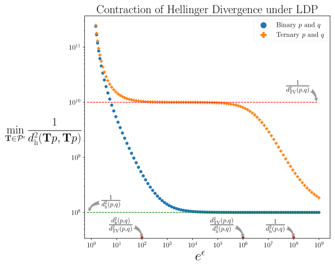
We highlight the differences between the sample complexity in the binary setting (cf. equation Equation 3) and the worst-case general distributions (cf. equation Equation 4) below (also see Figure 1):
-
1.
(Relaxing privacy may not lead to significant improvements in accuracy.) In equation Equation 4, there is an arbitrarily large range of where the sample complexity remains roughly constant. In particular, when , the sample complexity of hypothesis testing remains roughly the same (up to constants). That is, we are sacrificing privacy without any significant gains in statistical efficiency. This is in stark contrast to the binary setting, where increasing by a large constant factor leads to a constant-factor improvement in sample complexity.
-
2.
(The threshold for free privacy is larger.) Let be the threshold for free privacy (cf. Definition 1.4). In the binary setting, one has , whereas for general distributions, one may need . The former can be arbitrarily smaller than the latter.
To complement the result above, which provides a lower bound on the sample complexity for worst-case distributions, our next result provides an upper bound on the sample complexity that nearly matches the rates (up to logarithmic factors) for arbitrary distributions. Moreover, the proposed algorithm uses an -LDP channel with binary outputs. The following result is proved in Section 3.3:
Theorem 1.9 (Sample complexity upper bounds and an efficient algorithm for hypothesis testing for general distributions).
Let and be two distributions on . Let . Then the sample complexity behaves as
| (5) |
where .
Moreover, the rates above are achieved by an -LDP channel that maps to and can be found in time polynomial in , for any choice of , , and .
Theorems 1.7 and 1.9 imply that the above sample complexity is minimax optimal (up to logarithmic factors) over the class of distributions with total variation distance and Hellinger divergence satisfying the conditions in Theorem 1.7. We summarize this in the following theorem:
Theorem 1.10 (Minimax-optimal bounds).
Let and be such that . Let be the set of all distribution pairs with discrete supports, with total variation distance and Hellinger divergence being and , respectively:
Let be the minimax-optimal sample complexity of hypothesis testing under -LDP constraints, defined as
for test-rule pairs , as defined in Definition 1.3. Then
| (6) |
Here, the notation hides poly-logarithmic factors in and .
Remark 1.11.
A version of the above theorem may also be stated for privacy and communication constraints, by defining
In fact, it may seen that the same sample complexity bounds continue to hold for , with , since the lower bound in Theorem 1.7 continues to hold with communication constraints, as does the upper bound in Theorem 1.9, which uses a channel with only binary outputs.
Remark 1.12.
The above theorem mirrors a minimax optimality result for communication-constrained hypothesis testing from Pensia, Jog, and Loh [PJL23]. There, the set under consideration was , where is the Hellinger divergence between the distribution pair, and the minimax-optimal sample complexity was shown to be even for a binary communication constraint.
Finally, we consider the threshold for free privacy for general distributions; see Definition 1.4. Observe that Theorem 1.9 does not provide any upper bounds on , since the sample complexity in Theorem 1.9 is bounded away from , due to the logarithmic multiplier . Recall that Theorem 1.7 implies in the worst case. Our next result, proved in Section 3.3, shows that this is roughly tight, and for all distributions:
Theorem 1.13.
Let and be two distributions on , and let . Then . Moreover, there is a channel achieving this sample complexity that maps to a domain of size , and which can be computed in time.
We thereby settle the question of minimax-optimal sample complexity (up to logarithmic factors) for simple binary hypothesis testing under LDP-only and LDP-with-communication constraints (over the class of distributions with a given total variation distance and Hellinger divergence). Moreover, the minimax-optimal upper bounds are achieved by computationally efficient, communication-efficient algorithms. However, there can be a wide gap between instance-optimal and minimax-optimal procedures; in the next two subsections, we present structural and computational results for instance-optimal algorithms.
1.3.2 Structure of Extreme Points under the Joint Range
In this section, we present results for the extreme points of the joint range of an arbitrary pair of distributions when transformed by a set of channels. Formally, if is a convex set of channels from to , and and are two distributions on , we are interested in the extreme points of the set , which is a convex subset of .444For , we use to denote the probability simplex on a domain of alphabet size . Recall that a point is said to be an extreme point if cannot be expressed as a convex combination of two distinct points in ; i.e., if for , then . The extreme points of a convex set are naturally insightful for maximizing quasi-convex functions, and we will present the consequences of the results in this section in Section 1.3.3.
We consider two choices of : first, when is the set of all channels from to , and second, when is the set of all -LDP channels from to . We use to denote the set of all channels that map from to .
The following class of deterministic channels plays a critical role in our theory:
Definition 1.14 (Threshold channels).
For some , let and be two distributions on . For any , a deterministic channel is a threshold channel if the following property holds for every : If and , then any such that satisfies . (The likelihood ratios are assumed to take values on the extended real line; i.e., on .)
Remark 1.15.
Threshold channels are intuitively easy to understand when all the likelihood ratios are distinct (this may be assumed without loss of generality in our paper, as explained later): Arrange the inputs in increasing order of their likelihood ratios and partition them into contiguous blocks. Thus, there are at most such threshold channels (up to reordering of output labels).
Our first result proved in Section 4 is for the class of communication-constrained channels, and shows that all extreme points of the joint range are obtained using deterministic threshold channels:
Theorem 1.16 (Extreme points of the joint range under communication constraints).
Let and be two distributions on . Let be the set of all pairs of distributions that are obtained by passing and through a channel of output size , i.e.,
If is an extreme point of , then is a threshold channel.
We note that the above result is quite surprising: is extreme point of only if is an extreme point of (i.e., a deterministic channel), but Theorem 1.16 demands that be a deterministic threshold channel, meaning it lies in a very small subset of deterministic channels. Indeed, even for , the number of deterministic channels from to is , whereas the number of threshold channels is just . We note that the result above is similar in spirit to Tsitsiklis [Tsi93, Proposition 2.4]. However, the focus there was on a particular objective, the probability of error in simple hypothesis testing, with non-identical channels for users. Our result is for identical channels and is generally applicable to quasi-convex objectives, as mentioned later.
We now consider the case where is the set of -LDP channels from to . Since is a set of private channels, it does not contain any deterministic channels (thus, does not contain threshold channels). Somewhat surprisingly, we still show that the threshold channels play a fundamental role in the extreme points of the joint range under . The following result shows that any extreme point of the joint range can be obtained by a threshold channel mapping into , followed by an -LDP channel from to :
Theorem 1.17 (Extreme points of the joint range under privacy and communication constraints).
Let and be distributions on . Let be the set of -LDP channels from to . Let be the set of all pairs of distributions that are obtained by applying a channel from to and , i.e.,
| (7) |
If is an extreme point of for , then can be written as for some threshold channel and some an extreme point of the set of -LDP channels from to .
We prove this structural result in Section 5, which leads to polynomial-time algorithms for constant for maximizing quasi-convex functions, as mentioned in Section 1.3.3.
1.3.3 Computationally Efficient Algorithms for Instance Optimality
The results from the previous sections characterized the minimax-optimal sample complexity, but did not address instance optimality. Instance-optimal performance may be substantially better than minimax-optimal performance, as seen by comparing the instance-optimal bounds for binary distributions to the minimax-optimal bounds for general distributions. In this section, we focus on identifying an instance-optimal channel (satisfying the necessary constraints) for a given pair of distributions.
Let and be fixed distributions over . Let be the set of all -LDP channels from to , and let be the set of all channels from to . Let . As before, define . Let be a (jointly) quasi-convex function; i.e., for all , the sublevel sets are convex. In this paper, we are primarily interested in functions corresponding to divergences between the distribution pair. So, unless otherwise mentioned, we shall assume the quasi-convex functions in this paper are permutation-invariant; i.e., for all permutation matrices . However, our algorithmic results will continue to hold even without this assumption, with an additional factor of in the time complexity. We will consider the problem of identifying that solves
The quasi-convexity of implies that the maximum is attained at some such that is an extreme point of . We can thus leverage the results from Section 1.3.2 to search over the subset of channels satisfying certain structural properties.
Identifying that maximizes the Hellinger divergence leads to an instance-optimal test for minimizing sample complexity for testing between and with channel constraints : This is because if each user chooses the channel , the resulting sample complexity will be . Thus, the instance-optimal sample complexity will be obtained by a channel that attains . Note that the Hellinger divergence is convex (and thus quasi-convex) in its arguments. Apart from the Hellinger divergence, other functions of interest such as the Kullback–Leibler divergence or Chernoff information (which are also convex) characterize the asymptotic error rates in hypothesis testing, so finding for these functions identifies instance-optimal channels in the asymptotic (large-sample) regime. Other potential functions of interest include Rényi divergences of all orders, which are quasi-convex, but not necessarily convex [EH14].
As mentioned earlier, the results of Kairouz, Oh, and Viswanath [KOV16] give a linear program with variables to find an instance-optimal channel under privacy constraints, which is computationally prohibitive. It is also unclear if their result extends when the channels are further restricted to have communication constraints in addition to privacy constraints. We now show how to improve on the guarantees of Kairouz, Oh, and Viswanath [KOV16] in the presence of communication constraints, using the structural results from the previous subsection.
Corollary 1.18 (Computationally efficient algorithms for maximizing quasi-convex functions).
Let and be fixed distributions over , let , and let . Let be a jointly quasi-convex function. When , there is an algorithm that solves in time polynomial in . When , there is an algorithm that solves in time polynomial in and .
We prove Corollary 1.18 in Section 4 and Section 5.3 for and , respectively.
Remark 1.19.
When is constant, we obtain a polynomial-time algorithm for maximizing any quasi-convex function under or channel constraints. When and is the Kullback–Leibler divergence, this exactly solves (for small ) a problem introduced in Carpi, Garg, and Erkip [CGE21], which proposed a polynomial-time heuristic.
Applying the above result to the Hellinger divergence , we obtain the following result for simple binary hypothesis testing, proved in Section 5.3:
Corollary 1.20 (Computationally efficient algorithms for instance-optimal results under communication constraints).
Let and be two distributions on . For any and any integer , there is an algorithm that runs in time polynomial in and and outputs an -LDP channel mapping from to , such that if denotes the sample complexity of hypothesis testing between and when each individual uses the channel , then .
In particular, the sample complexity with satisfies
| (8) |
The channel may be decomposed as a deterministic threshold channel to a domain of size , followed by an -LDP channel from to .
Thus, by choosing , we obtain a polynomial-time algorithm with nearly instance-optimal sample complexity (up to logarithmic factors) under just -LDP constraints.
1.4 Related Work
Distributed estimation has been studied extensively under resource constraints such as memory, privacy, and communication. Typically, this line of research considers problems of interest such as distribution estimation [RT70, LR86, CKO21, BHÖ20], identity or independence testing [ACT20, ACT20a, ACFST21], and parameter estimation [Hel74, DJWZ14, DJW18, BGMNW16, DR19, BCÖ20, DKPP22], and identifies minimax-optimal bounds on the error or sample complexity. In what follows, we limit our discussion to related work on hypothesis testing under resource constraints.
For memory-constrained hypothesis testing, the earliest works in Cover [Cov69] and Hellman and Cover [HC73] derived tight bounds on the memory size needed to perform asymptotically error-free testing. Hellman and Cover [HC71] also highlighted the benefits of randomized algorithms. These benefits were also noted in recent work by Berg, Ordentlich, and Shayevitz [BOS20], which considered the error exponent in terms of the memory size. Recently, Braverman, Garg, and Zamir [BGZ22] showed tight bounds on the memory size needed to test between two Bernoulli distributions.
Communication-constrained hypothesis testing has two different interpretations. In the information theory literature, Berger [Ber79], Ahlswede and Csiszár [AC86], and Amari and Han [AH98] considered a family of problems where two nodes, one which only observes ’s and the other which only observes ’s, try to distinguish between and . Communication between the nodes occurs over rate-limited channels. The second interpretation, also called “decentralized detection” in Tsitsiklis [Tsi88], is more relevant to this work. Here, the observed ’s are distributed amongst different nodes (one observation per node) that communicate a finite number of messages (bits) to a central node, which needs to determine the hypothesis. Tsitsiklis [Tsi88, Tsi93] identified the optimal decision rules for individual nodes and considered asymptotic error rates in terms of the number of bits. These results were recently extended to the nonasymptotic regime in Pensia, Jog, and Loh [PJL23, PLJ22].
Privacy-constrained hypothesis testing has been studied in the asymptotic and nonasymptotic regimes under different notions of privacy. The local privacy setting, which is relevant to this paper, is similar to the decentralized detection model in Tsitsiklis [Tsi93], except that the each node’s communication to the central server is private. This is achieved by passing observations through private channels. Liao, Sankar, Calmon, and Tan [LSCT17, LSTC17] considered maximizing the error exponent under local privacy notions defined via maximal leakage and mutual information. Sheffet [She18] analyzed the performance of the randomized response method for LDP for hypothesis testing. Gopi, Kamath, Kulkarni, Nikolov, Wu, and Zhang [GKKNWZ20] showed that -ary hypothesis testing under pure LDP constraints requires exponentially more samples ( instead of ). Closely related to the instance-optimal algorithms in our paper, Kairouz, Oh, and Viswanath [KOV16] presented an algorithm to find LDP channels that maximize the output divergence for two fixed probability distributions at the channel input; the proposed algorithm runs in time exponential in the domain size of the input distributions.555We remark, however, that the algorithm in Kairouz, Oh, and Viswanath [KOV16] is applicable to a wider class of objective functions, which they term “sublinear.” Note that divergences are directly related to error exponents and sample complexities in binary hypothesis testing. The results of Kairouz, Oh, and Viswanath [KOV16] on extreme points of the polytope of LDP channels were strengthened in Holohan, Leith, and Mason [HLM17], which characterized the extreme points in special cases. We were able to find only two other papers that consider instance optimality, but in rather special settings [GGKMZ21, AFT22]. For simple binary hypothesis testing in the global differential privacy setting, Canonne, Kamath, McMillan, Smith, and Ullman [CKMSU19] identified the optimal test and corresponding sample complexity. Bun, Kamath, Steinke, and Wu [BKSW19] showed that samples are enough for -ary hypothesis testing in the global differential privacy setting.
1.5 Organization
This paper is organized as follows: Section 2 records standard results. Section 3 focuses on the sample complexity of hypothesis testing under privacy constraints. Section 4 considers extreme points of the joint range under communication constraints. Section 5 characterizes the extreme points under both privacy and communication constraints. Section 6 explores other notions of privacy beyond pure LDP. Finally, we conclude with a discussion in Section 7. We defer proofs of some intermediate results to the appendices.
2 Preliminaries and Facts
Notation:
Throughout this paper, we will focus on discrete distributions. For a natural number , we use to denote the set and to denote the set of distributions over . We represent a probability distribution as a vector in . Thus, denotes the probability of element under . Given two distributions and , let and denote the total variation distance and Hellinger divergence between and , respectively.
We denote channels with bold letters such as . As the channels between discrete distributions can be represented by rectangular column-stochastic matrices (each column is nonnegative and sums to one), we also use bold capital letters, such as , to denote the corresponding matrices. In particular, if a channel is from to , we denote it by an matrix, where each of the columns is in . In the same vein, for a column index and a row index , we use to refer to the entry at the corresponding location. For a channel and a distribution over , we use to denote the distribution over when passes through the channel . In the notation above, when is a distribution over , represented as a vector in , and is a channel from , represented as a matrix , the output distribution corresponds to the usual matrix-vector product. We shall also use to denote the stochastic map transforming the channel input to the channel output . Similarly, for two channels and from to and to , respectively, the channel from to that corresponds to applying to the output of is equal to the matrix product .
Let be the set of all channels that map from to . We use to denote the subset of that corresponds to threshold channels (cf. Definition 1.14). We use to denote the set of all -LDP channels from to . Recall that for two distributions and , we use (respectively, ) to denote the sample complexity of simple binary hypothesis testing under privacy constraints (respectively, both privacy and communication constraints).
For a set , we use to denote the convex hull of . For a convex set , we use to denote the set of extreme points of . Finally, we use the following notations for simplicity: (i) , , and to hide positive constants, and (ii) the standard asymptotic notation , , and . Finally, we use , , and to hide poly-logarithmic factors in their arguments.
2.1 Convexity
We refer the reader to Bertsimas and Tsitsiklis [BT97] for further details. We will use the following facts repeatedly in the paper, often without mentioning them explicitly:
Fact 2.1 (Extreme points of linear transformations).
Let be a convex, compact set in a finite-dimensional space. Let be a linear function on , and define the set . Then is convex and compact, and .
Fact 2.2.
Let be a convex, compact set. If for some set , then .
Fact 2.3 (Number of vertices and vertex enumeration).
Let be a bounded polytope defined by linear inequalities. The number of vertices of is at most . Moreover, there is an algorithm that takes time and output all the vertices of .666Throughout this paper, we assume the bit-complexity of linear inequalities is bounded.
Fact 2.4 (Extreme points of channels).
The set of extreme points of is the set of all deterministic channels from to .
2.2 Local Privacy
We state standard facts from the privacy literature here.
Definition 2.5 (Randomized response).
For an integer , the -ary randomized response channel with privacy parameter is a channel from to defined as follows: for any , with probability and with probability , for any . The standard randomized response [War65] corresponds to , which we denote by . We omit in the superscript when it is clear from context.
We will also use the following result on the extreme points for Theorem 1.7.
Fact 2.6 (Extreme points of the LDP polytope in special cases [HLM17]).
We mention all the extreme points of (up to permutation of rows and columns; if a channel is an extreme point, then any permutation of rows and/or columns is an extreme point) below for some special cases.
-
1.
(Trivial extreme points) A channel with one row of all ones and the rest of the rows with zero values is always an extreme point of . We call such extreme points trivial.
-
2.
( and ) All non-trivial extreme points of are of the form (up to permutation of rows):
where . In other words, the columns are of only two types, containing and .
2.3 Hypothesis Testing
In this section, we state some standard facts regarding hypothesis testing and divergences that will be used repeatedly.
Fact 2.7 (Hypothesis testing and divergences; see, for example, Tsybakov [Tsy09]).
Let and be two arbitrary distributions. Then:
-
1.
We have .
-
2.
(Sample complexity of non-private hypothesis testing) We have .
- 3.
-
4.
(Restricting the size of the output domain) Let and be distributions over . Then . This follows by applying Theorem 2 in Kairouz, Oh, and Viswanath [KOV16] to .
-
5.
(Choice of identical channels in Definition 1.2) Let be a channel that maximizes among all channels in . Then the sample complexity of hypothesis testing under the channel constraints of is . See Lemma 4.2 in Pensia, Jog, and Loh [PJL23].
Fact 2.8 (Preservation of Hellinger distance under communication constraints (Theorem 1 in Bhatt, Nazer, Ordentlich, and Polyanskiy [BNOP21] and Corollary 3.4 in Pensia, Jog, and Loh [PJL23])).
Let and be two distributions on . Then for any , there exists a channel from to , which can be computed in time polynomial in , such that
| (9) |
Moreover, this bound is tight in the following sense: for every choice of , there exist two distributions and such that , and for every channel , the right-hand side of inequality Equation 9 is further upper-bounded by .
3 Locally Private Simple Hypothesis Testing
In this section, we provide upper and lower bounds for locally private simple hypothesis testing. This section is organized as follows: In Section 3.1, we derive instance-optimal bounds when both distributions are binary. We then prove minimax-optimal bounds for general distributions (with support size at least three): Lower bounds on sample complexity are proved in Section 3.2 and upper bounds in Section 3.3. Proofs of some of the technical arguments are deferred to the appendices.
3.1 Binary Distributions and Instance-Optimality of Randomized Response
We first consider the special case when and are both binary distributions. Our main result characterizes the instance-optimal sample complexity in this setting: See 1.6 By Fact 2.7, the proof of Theorem 1.6 is a consequence of the following bound on the strong data processing inequality for randomized responses:
Proposition 3.1 (Strong data processing inequality for Hellinger divergence).
Let and be two binary distributions. Then
Moreover, the maximum is achieved by the randomized response channel.
Proof.
Let be the joint range of and under -LDP privacy constraints. Since is a convex set and is a convex function over , the maximizer of in is an extreme point of . Since is a linear transformation of , Fact 2.1 implies that any extreme point of is obtained by using a channel corresponding to an extreme point of . By Fact 2.6, the only extreme point of is the randomized response channel . Thus, in the rest of the proof, we consider .
By abusing notation, we will also use and to denote the probabilities of observing under the two respective distributions. Without loss of generality, we will assume that and . We will repeatedly use the following claim, which is proved in Appendix D:
Claim 3.2 (Approximation for Hellinger divergence of binary distributions).
Let . Let and be the corresponding Bernoulli distributions with . Then
Applying Claim 3.2, we obtain
| (10) |
We know that the transformed distributions and are binary distributions; by abusing notation, let and also be the corresponding real-valued parameters associated with these binary distributions. By the definition of the randomized response, we have
| (11) |
Consequently, we have and . We directly see that
We now apply Claim 3.2 below to the distributions and :
where the last step uses the inequality from Fact 2.7. ∎
3.2 General Distributions: Lower Bounds and Higher Cost of Privacy
In this section, we establish lower bounds for the sample complexity of private hypothesis testing for general distributions. In the subsequent section, the lower bounds will be shown to be tight up to logarithmic factors.
We formally state the lower bound in the statement below: See 1.7 We provide the proof below. We refer the reader to Remark 1.8 for further discussion on differences between the worst-case sample complexity of general distributions and the sample complexity of binary distributions (cf. Theorem 1.6). We note that a similar construction is mentioned in Canonne, Kamath, McMillan, Smith, and Ullman [CKMSU19, Section 1.3]; however, their focus is on the central model of differential privacy.
3.2.1 Proof of Theorem 1.7
Proof.
The case when follows from Fact 2.7. Thus, we set in the remainder of this section. We start with a helpful approximation for computing the Hellinger divergence, proved in Appendix D:
Claim 3.3 (Additive approximation for ).
There exist constants such that for , we have .
For some and to be decided later, let and be the following ternary distributions:
Since and , these two are valid distributions.
Observe that and and by Claim 3.3. We choose and such that and . Such a choice of and can be made by the argument given in Section D.2 as long as and . Thus, these two distributions satisfy the first two conditions of the theorem statement.
In the rest of the proof, we will use the facts that and . In particular, we have .
Since both and are supported on [3], we can restrict our attention to ternary output channels (see Fact 2.7). In fact, we can go a step further and restrict our attention to only binary output channels. This is because, suppose we have a ternary output channel with corresponding output distributions being . There exists some such that . Consider a channel that maps to [2] deterministically, by sending to 1 and to 2. Set . We note two facts: (i) , and (ii) is an -private channel from [3] to [2] because of the composition property of private channels. In other words, for every -private channel from [3] to [3], there exists an -private channel from [3] to [2] that has the same output Hellinger distance (up to multiplicative constants). Thus,
We will establish the following result: for all such that , we have
| (12) |
By Fact 2.7, equation Equation 12 implies that for , we have
| (13) |
Let be the right endpoint of the range for above, i.e., . Then equation Equation 13 shows that . Since for any such that , we have , the desired conclusion in equation Equation 4 holds for , as well. Thus, in the remainder of this proof, we will focus on establishing equation Equation 12.
Since is a convex, bounded function and the set of -LDP channels is a convex polytope, it suffices to restrict our attention only to the extreme points of the polytope. As mentioned in Fact 2.6, these extreme points are of two types:
-
Case I.
(Trivial extreme point) Any such extreme point maps the entire domain to a single point with probability . After transformation under this channel, all distributions become indistinguishable, giving .
-
Case II.
(Deterministic binary channel cascaded with the randomized response channel) This corresponds to the case when , where is a deterministic threshold channel from to .777We use Theorem 1.17 to restrict our attention only to threshold channels. There are two non-trivial options for choosing , which we analyze below.
The first choice of maps and to different elements. The transformed distributions and are and , respectively. Using Claim 3.3, we obtain and . Let and be the corresponding distributions after applying the randomized response with parameter . Since and are binary distributions, we can apply Proposition 3.1 to obtain
which is equal to in the regime of interest and consistent with the desired expression in equation Equation 12.
The second choice of maps and to different elements. The transformed distributions and are and , respectively. Applying Claim 3.3, we observe that and . Let and be the corresponding distributions after applying the randomized response with parameter . Applying Proposition 3.1, we obtain
in the regime of interest. Again, this is consistent with equation Equation 12.
Combining the cases above, the maximum Hellinger divergence after applying any -LDP channel is , as desired. ∎
3.3 General Distributions: Upper Bounds and Minimax Optimality
We now demonstrate an algorithm that finds a private channel matching the minimax rate in Theorem 1.7 up to logarithmic factors. Moreover, the proposed algorithm is both computationally efficient and communication efficient.
See 1.9 In comparison with Theorem 1.7, we see that the test above is minimax optimal up to logarithmic factors over the class of distributions with fixed Hellinger divergence and total variation distance. The channel satisfying this rate is of the following simple form: a deterministic binary channel , followed by the randomized response. In fact, we can take to be either Scheffe’s test (which preserves the total variation distance) or the binary channel from Fact 2.8 (which preserves the Hellinger divergence), whichever of the two is better. We provide the complete proof in Section 3.3.1.
One obvious shortcoming of Theorem 1.9 is that even when , the test does not recover the optimal sample complexity of , due to the logarithmic multiplier . We now consider the case when and exhibit a channel that achieves the optimal sample complexity as soon as . Thus, privacy can be attained essentially for free in this regime.
See 1.13
We note that the size of the output domain of is tight in the sense that any channel that achieves the sample complexity within constant factors of must use an output domain of size at least ; this follows by the tightness of Fact 2.8 in the worst case. Consequently, the channel achieving the rate above is roughly of the form (1) a communication-efficient channel from Fact 2.8 that preserves the Hellinger divergence up to constant factors, followed by (2) an -ary randomized response channel, for .
We give the proof of Theorem 1.13 in Section 3.3.2 and defer the proofs of some of the intermediate results to Appendix A.
3.3.1 Proof of Theorem 1.9
In this section, we provide the proof of Theorem 1.9. We first note that this result can be slightly strengthened, replacing by , where is the sample complexity of hypothesis testing under binary communication constraints. This choice of is smaller, by Pensia, Jog, and Loh [PJL23, Corollary 3.4 and Theorem 4.1].
Proof.
The case of follows from Fact 2.7; thus, we focus on the setting where .
We will establish these bounds via Proposition 3.1, by using a binary deterministic channel, followed by the binary randomized response channel. A sample complexity of is direct by using the channel for . Thus, our focus will be on the term .
Let be a deterministic binary output channel to be decided later. Consider the channel . By Proposition 3.1, we have
| (14) |
where the first inequality uses Fact 2.7
If we choose the channel from Fact 2.8, we have . Applying this to inequality Equation 14, we obtain
By Fact 2.7, the sample complexity of , which is -LDP, is at most , which is equivalent to the desired statement.
Finally, the claim on the runtime is immediate, since the channel from Fact 2.8 can be found efficiently. ∎
3.3.2 Proof of Theorem 1.13
We will prove a slightly generalized version of Theorem 1.13 below that works for a wider range of :
Proposition 3.4.
Let and be two distributions on and . Then there exists an -LDP channel from to , for , such that
Furthermore, the channel can be be computed in time.
By Fact 2.7, Proposition 3.4 implies the following:
where . Setting equal to proves Theorem 1.13. Thus, we will focus on proving Proposition 3.4 in the rest of this section. We establish this result with the help of the following observations:
-
•
(Lemma 3.5) First, we show that the randomized response preserves the contribution to the Hellinger divergence by “comparable elements” (elements whose likelihood ratio is in the interval ) when is large compared to the support size. In particular, we first define the following sets:
(15) Let denote the randomized response channel from to with privacy parameter (cf. Definition 2.5). The following result is proved in Section A.1:
Lemma 3.5 (Randomized response preserves contribution of comparable elements).
Let and be two distributions on . Suppose . Then , for , satisfies
Thus, when , the randomized response preserves the original contribution of comparable elements.
-
•
(Lemma 3.6) We then show in Lemma 3.6, proved in Section A.2, that either we can reduce the problem to the previous special case (small support size and main contribution to Hellinger divergence is from comparable elements) or to the case when the distributions are binary (where Proposition 3.1 is applicable and is, in a sense, the easy case for privacy).
Lemma 3.6 (Reduction to base case).
Let and be two distributions on . Then there is a channel , which can be computed in time polynomial in , that maps to (for to be decided below) such that for and , at least one of the following holds:
-
1.
For any and , we have
where and are defined analogously to and in equation Equation 15, but with respect to distributions and .
-
2.
and .
-
1.
We now provide the proof of Proposition 3.4, with the help of Lemmata 3.5 and 3.6.
Proof.
(Proof of Proposition 3.4) The channel will be of the form , where is a channel from to and is to be decided. The privacy of is clear from the construction.
We begin by applying Lemma 3.6. Let be the channel from Lemma 3.6 that maps from to . Let and , and define and . The claim on runtime thus follows from Lemma 3.6.
Suppose for now that from Lemma 3.6 is a binary channel. Then we know that and , where the latter holds by Fact 2.7. Applying Proposition 3.1, we have
which concludes the proof in this case.
We now consider the case when in the guarantee of Lemma 3.6. Then the comparable elements of and preserve a significant fraction of the Hellinger divergence (depending on the chosen value of ) between and . Let , and choose to be . Then Lemma 3.6 implies that the contribution to the Hellinger divergence from comparable elements of and is at least , for . We will now apply Lemma 3.5 to and with the above choice of . Since by construction, applying Lemma 3.5 to and , we obtain
where the last step uses the facts that and . This completes the proof. ∎
4 Extreme Points of Joint Range Under Communication Constraints
In this section, our goal is to understand the extreme points of the set . This will allow us to identify the structure of optimizers of quasi-convex functions over . The main result of this section is the following: See 1.16
We provide the proof of Theorem 1.16 in Section 4.1. Before proving Theorem 1.16, we discuss some consequences for optimizing quasi-convex functions over . The following result proves Corollary 1.18 for :
Corollary 4.1 (Threshold channels maximize quasi-convex functions).
Let and be two distributions on . Let . Let be a real-valued quasi-convex function over . Then
Moreover, the above optimization problem can be solved in time .888Recall that is assumed to be permutation invariant. If not, an extra factor of will appear in the time complexity.
Proof.
Observe that is a closed polytope. Let be the set of extreme points of . Observe that , and thus is finite. Since is a closed polytope, is convex hull of . Furthermore, the maximum of on is well-defined and finite, as is a finite set. Any can be expressed as a convex combination . Recall that an equivalent definition of quasi-convexity is that satisfies for all . By repeatedly using this fact, we have
By Theorem 1.16, any extreme point is obtained by passing and through a threshold channel. Thus, the maximum of over is attained by passing and through a threshold channel. The claimed runtime is obtained by trying all possible threshold channels. ∎
Remark 4.2.
(Quasi-)convex functions of interest include all -divergences, Rényi divergences, Chernoff information, and norms. We note that the above result also holds for post-processing: For any fixed channel , we have
This is because is a quasi-convex function of .
Remark 4.3.
If is the Hellinger divergence and , we can conclude the following result for the communication-constrained setting: There exists a that attains the instance-optimal sample complexity (up to universal constants) for hypothesis testing under a communication constraint of size . This result is implied in Pensia, Jog, and Loh [PJL23] by Theorem 2.9 (which is a result from Tsitsiklis [Tsi93]) and Lemma 4.2. The above argument provides a more straightforward proof.
4.1 Proof of Theorem 1.16
We now provide the proof of Theorem 1.16.
Proof.
(Proof of Theorem 1.16) We first make the following simplifying assumption about the likelihood ratios: there is at most a single element with , and for all other elements , is a unique value. If there are two or more elements with the same likelihood ratio, we can merge those elements into a single alphabet without loss of generality, as we explain next. Let and be the distributions after merging these elements, and let be the new cardinality. Then for any channel , there exists another channel such that . We can then apply the following arguments to and . See Section D.1 for more details.
In the following, we will consider to be if , and we introduce the notation . We will further assume, without loss of generality, that is strictly increasing in . Since the elements are ordered with respect to the likelihood ratio, a threshold channel corresponds to a map that partitions the set into contiguous blocks. Formally, we have the following definition:
Definition 4.4 (Partitions and threshold partitions).
We say that forms an -partition of if and for . We say that forms an -threshold partition of if in addition, for all , every entry of is less than every entry of .
As mentioned before, channels corresponding to -threshold partitions are precisely the threshold channels up to a permutation of output labels. The channels corresponding to -partitions are the set of all deterministic channels that map to , which are the extreme points of (cf. Fact 2.4).
Observe that is a convex, compact set, which is a linear transformation of the convex, compact set , and any extreme point of is of the form , where is an extreme point of (cf. Fact 2.1). Now suppose is an extreme point of , but is not a threshold channel. Thus, corresponds to some -partition of that is not an -threshold partition. We will now show that is not an extreme point of , by showing that there exist two distinct channels and such that the following holds:
| (16) |
and .
Since is not a -threshold partition, there exist and in such that and , and . Among , and , only is potentially zero. Suppose for now that ; we will consider the alternative case shortly.
For some and to be determined later, let be the following channel:
-
1.
For , maps to .
-
2.
For (respectively ), maps to (respectively ) with probability (respectively ) and to (respectively ) with probability (respectively ).
Thus, the channels and have all columns identical, except for those corresponding to inputs and . Let be the column of . Observe that is a degenerate distribution at and is a degenerate distribution at (equivalently, and ). Thus, we can write
If we choose , we have and
| (17) |
Recall that , as mentioned above.
We now define . For some and to be decided later, we have:
-
1.
For , maps to .
-
2.
For (respectively ), maps to (respectively ) with probability (respectively ) and to (respectively ) with probability (respectively ).
With the same arguments as before, we have
If we choose , we have and
| (18) |
where the last line follows by the fact that , since maps both and to almost surely.
Let and be such that . Such a choice always exists because and are both strictly positive and finite. Then equations Equation 17 and Equation 18 imply that and , and . Moreover, . Thus, is not an extreme point of .
We now outline how to modify the construction above when is zero. By setting to be zero, we obtain and . The desired conclusion follows by choosing and small enough such that .
∎
5 Extreme Points of Joint Range under Privacy Constraints
In the previous section, we considered the extreme points of the joint range under communication constraints. Such communication constraints are routinely applied in practice in the presence of additional constraints such as local differential privacy. However, the results of the previous section do not apply directly, as the joint range is now a strict subset of the set in Theorem 1.16, and the extreme points differ significantly. For example, the threshold channels are not even private. However, we show in this section that threshold channels still play a fundamental role. Our main result in this section is the following theorem:
See 1.17
Actually, our result applies to a broader family of linear programming (LP) channels that we describe below:
Definition 5.1 (LP family of channels).
For any , let and be two nonnegative vectors in . For , define the set of linear programming (LP) channels , a subset of , to be the (convex) set of all channels from to that satisfy the following constraints:
| (19) |
When and for all , we recover the set of -LDP channels from to . Another example will be mentioned in Section 6 for a relaxed version of approximate LDP.
The rest of this section is organized as follows: In Section 5.1, we show that any that leads to an extreme point of cannot have more than unique columns (Lemma 5.2). We use this result to prove Theorem 1.17 in Section 5.2. In Section 5.3, we apply Theorem 1.17 to prove Corollaries 1.18 and 1.20.
5.1 Bound on the Number of Unique Columns
The following result will be critical in the proof of Theorem 1.17, the main result of this section.
Lemma 5.2.
Let and be distributions on . Let be the set of channels from to , from Definition 5.1. Let be the set of all pairs of distributions that are obtained by applying a channel from to and , i.e.,
| (20) |
If has more than unique columns, then is not an extreme point of .
We prove this result in Section 5.1.2 after proving a quantitatively weaker, but simpler, result in Section 5.1.1.
5.1.1 Warm-Up: An Exponential Bound on the Number of Unique Columns
In this section, we first prove a weaker version of Lemma 5.2, where we upper-bound the number of unique columns in the extreme points of from Definition 5.1 (not just those that lead to extreme points of ) by an exponential in . In fact, this bound will be applicable for a broader class of channels that satisfy the following property:
Condition 5.3 (Only one free entry per column).
Let be a convex set of channels from to . Let be an extreme point of . Then there exist numbers and such that for every column , there exists at most a single row such that . We call such entries free.
We show in Appendix B that extreme points of the LP channels from Definition 5.1 satisfy Condition 5.3. The following claim bounds the number of unique columns in any extreme point of , and thus also implies a version of Theorem 1.17 with instead of (cf. Fact 2.1).
Claim 5.4 (Number of unique columns in an extreme point is at most exponential in ).
Let be a set of channels satisfying the property of Condition 5.3. Let be an extreme point of . Then the number of unique columns in is at most . In particular, can be written as , where is a deterministic map from to and is a map from to , for .
Proof.
We use the notation from Condition 5.3. For each column, there are possible locations of a potential free entry. Let this location be ; the value at this location is still flexible. Now let us consider the number of ways to assign values at the remaining locations. For each , the entry is either or (since is not a free entry). Thus, there are such possible assignments. Since the column entries sum to one, each of those assignments fixes the value at the location, as well. Thus, there are at most unique columns in . ∎
5.1.2 Forbidden Structure in Extreme Points Using the Joint Range
In Claim 5.4, we considered the extreme points of LP channels. However, we are actually interested in a (potentially much) smaller set: the extreme points that correspond to the extreme points of the joint range . In this section, we identify a necessary structural property for extreme points of LP channels that lead to extreme points of the joint range. We begin by defining the notion of a “loose” entry in a channel in :
Definition 5.5 (Loose and tight entries).
Let be a channel in from Definition 5.1 that maps from to . Let and be the row-wise minimum and maximum entries, respectively. For and , we say an entry is max-tight if and . An entry is min-tight if and . An entry that is neither max-tight nor min-tight is called loose.
Remark 5.6.
Our results in this section continue to hold for a slightly more general definition, where we replace the linear functions by arbitrary monotonically increasing functions . We focus on linear functions for simplicity and clarity. (Also see Remark 5.11.)
If the rest of the row is kept fixed, a max-tight entry cannot be increased without violating privacy constraints, but it can be decreased. Similarly, a min-tight entry cannot be decreased without violating privacy constraints, but it can be increased. Loose entries can be either increased or decreased without violating privacy constraints. These perturbations need to be balanced by adjusting other entries in the same column to satisfy column stochasticity; for example, a max-tight entry can be decreased while simultaneously increasing a min-tight or loose entry in the same column. This is formalized below:
Condition 5.7 (Mass can be transferred from entries that are not tight).
Let be a set of channels from to . Let be any extreme point of . Suppose there are two rows and two columns (in the display below, we take and without loss of generality) with values , as shown below:
such that:
-
•
and are not min-tight ( and above, respectively).
-
•
and are not max-tight ( and above, respectively).
Then there exist and such that for all and , the following matrix also belongs to :
where the omitted entries of and are the same.
We show that the channels from Definition 5.1 satisfy Condition 5.7 in Appendix B. Using Condition 5.7, we show that the following structure is forbidden in the channels that lead to extreme points of the joint range:
Lemma 5.8.
Let and be two distributions on . Let be the set of LP channels from Definition 5.1 (or, more generally, a convex set of channels satisfying Condition 5.7) from to . Suppose is strictly increasing in . Let have the following structure: there are two rows (in the display below, is taken without loss of generality) and three columns with values , as shown below:
such that:
-
•
and are not min-tight ( and above, respectively).
-
•
and are not max-tight ( and above, respectively).
Let . Then cannot be an extreme point of .
Proof.
Firstly, the set is convex since is convex. For some and to be decided later, consider the following perturbed matrices:
To be specific, the entries of , , and match except in the six locations highlighted here. Since satisfies Condition 5.7 (see Claim B.2), both and belong to the set if , , , and are small enough and positive. We will now show that there exist choices of these parameters such that is a convex combination of and , and these three points are distinct elements of . Consequently, will not be an extreme point of .
For any , let denote the vector in that is at the location and otherwise. Define to be the likelihood ratio. If , then . Since is strictly increasing in , only may be infinity. Let us first suppose that . We will consider the case when might be infinity in the end.
Let us begin by analyzing how transforms and . Since differs from only in the four locations mentioned above, and , both of which are distributions on , differ only in the elements and of . On the element , is equal to , and equal to its negation on the element . In particular, they satisfy the relation
If , we have . Under the same setting, is transformed as follows:
We now analyze the effect of , which satisfies
If , we have . Under the same setting, is transformed as follows:
Now observe that . By choosing and small enough such that , we obtain
and all three points are distinct elements of . Such a choice of and always exists, since both and are positive and finite. Thus, is not an extreme point of .
Let us now consider the case when , or equivalently, . Define to be , so that and . Then choose and small enough such that , which is possible since both sides are positive and finite. Thus, is a non-trivial convex combination of and , so is not an extreme point of . ∎
5.1.3 Proof of Lemma 5.2
Proof.
Without loss of generality, we assume that the likelihood ratios are unique and strictly increasing in . We refer the reader to the proof of Theorem 1.16 and Claim D.1 for more details.
Let be a channel from to such that is an extreme point of . Suppose that there are unique columns in with . From now on, we assume that ; otherwise, we apply the following argument to the first distinct columns.
Let be such that the and columns of are distinct. Observe that for every pair of distinct columns and , there are two rows such that column has a strictly bigger value than the column on one row, and vice versa on the another row. This is because both of the columns sum up to , so if a particular column has a larger entry in a row, its entry must be smaller in a different row. In particular, there exist two rows and such that and . As a result, and are not min-tight, and and are not max-tight.
We now order the distinct columns of in the order of their appearance from left to right. Let be the indices of the unique columns. For example, the first distinct column is the first column of (corresponding to the element ). The second distinct column is the first column of that is different from the first column. The third distinct column is the first column of that is different from the first two columns. Let be the set of unique column indices of .
Now, we divide the distinct columns in into pairs: . The total number of possible choices in is , and for every in , the possible number of choices of is at most , since both of these lie in and are distinct. Thus, there must exist two pairs in whose corresponding indices are the same, since .
Without loss of generality, we let these pairs of columns be and . Let and . Then the previous discussion implies that:
-
•
and are not min-tight, and and are not max-tight.
-
•
and are not max-tight, and and are not min-tight.
Thus, the columns , and satisfy the conditions of Lemma 5.8, i.e., they exhibit the forbidden structure. This implies that cannot be an extreme point of . Therefore, . ∎
5.2 Proof of Theorem 1.17: Unique Columns to Threshold Channels
In this section, we provide the proof of Theorem 1.17 using Lemma 5.2. Noting that our main structural result is more widely applicable (Condition 5.7), we prove a more general version of Theorem 1.17 below for Definition 5.1. Before doing so, we require an additional property on the set of our channels, proved in Appendix B:
Claim 5.9 (Closure under pre-processing).
The set satisfies the following closure property under pre-processing:
| (21) |
Informally, if we take an arbitrary channel and compose it with an LP private channel , the composition is also LP private.
The following result is thus a more general version of Theorem 1.17:
Theorem 5.10 (Structure of optimal channels).
Let and be distributions on . For any , let be the set of channels from Definition 5.1. Let be the set of all pairs of distributions that are obtained by applying a channel from to and , i.e.,
| (22) |
If is an extreme point of , then can be written as , for some and an extreme point of the set .
Proof.
Since is convex, the joint range is convex. By Lemma 5.2, we know that if is an extreme point of , then can be written as , where for . Using Claim 5.9, any such channel in is of the form , where and . Combining the last two observations, we obtain the following:
| (23) |
We now claim that we can further take to be a threshold channel and to be an extreme point of . This claim follows if we can write an arbitrary point in as a convex combination of elements of the set . By equation Equation 23, it suffices to demonstrate this convex combination for all points of the form , for some and .
Let be extreme points of , and let be an enumeration of the threshold channels . By definition, any can be written as for some convex combination . Furthermore, Theorem 1.16 implies that any , for , can be written as , for some convex combination .
Thus, any arbitrary point , for and , can be written as
Finally, note that are also valid convex combinations of , since they are nonnegative and sum to . ∎
Remark 5.11 (Extending Theorems 5.10 and 1.17 to a more general set of constraints).
We note that Theorem 5.10 can be extended to an arbitrary convex set of channels that satisfy (appropriately modified versions of) Condition 5.7 and equation Equation 21. (Also see Remark 5.6.)
5.3 Application to Hypothesis Testing
In Section 3, we showed that the minimax-optimal sample complexity can be obtained by a communication-efficient and efficiently computable channel, up to logarithmic factors. However, for a particular , these guarantees can be significantly improved. For example, consider the extreme case when and are the following two distributions on : for small enough,
Let be a deterministic binary channel that maps the first and second elements to different elements, while assigning the remaining elements arbitrarily. Now consider the following private channel : the channel , followed by the randomized response over binary distributions. Then as , the performance of mirrors equation Equation 3, which is much better than the minimax bound of equation Equation 4. Thus, there is a wide gap between instance-optimal and minimax-optimal performance. We thus consider the computational question of optimizing a quasi-convex function over all possible -private channels that map to a domain of size .
The following result proves Corollary 1.18 for equal to :
Corollary 5.12 (Computationally efficient algorithms for maximizing quasi-convex functions under privacy constraints).
Let and be fixed distributions over , let be the set of channels from Definition 5.1, and let . Let be a jointly quasi-convex function. Then there is an algorithm that solves in time polynomial in and .999Recall that is assumed to be permutation invariant. If not, an extra factor of will appear in the time complexity.
Proof.
The algorithm is as follows: we try all threshold channels in and all extreme points of , and output the channel that attains the maximum value of . By Theorem 5.10 and quasi-convexity of , we know the algorithm will output a correct value, since all extreme points are of this form. Thus, we focus on bounding the runtime. We know that the cardinality of is bounded by (up to a rotation of output rows). By Fact 2.3, the time taken to iterate through all the extreme points of -LDP channels from to is at most polynomial in , since is a polytope in with inequalities. This completes the proof. ∎
The proof of Corollary 1.20 is immediate from Fact 2.7, Corollary 1.18, and Proposition 6.2, stated later.
6 Extensions to Other Notions of Privacy
In this section, we explore computational and statistical aspects of hypothesis testing under other notions of privacy. Section 6.1 is on approximate privacy, in which we first focus on -LDP and then our proposed definition of approximate privacy. Next, we focus on binary communication constraints for Rényi differential privacy in Section 6.2. This will be possible since our algorithmic and structural results were not restricted to the case of pure LDP.
We begin by noting that communication constraints have a benign effect on the sample complexity of hypothesis testing for many notions of privacy:
Condition 6.1 (Closure under post-processing).
Let . For each , consider sets and define . We say satisfies -post-processing if for every , if and is a deterministic channel from to , the channel also belongs to , and thus to .
Post-processing is satisfied by various notions of privacy: -pure privacy, -approximate privacy (see Dwork and Roth [DR13, Proposition 2.1]), and Rényi privacy [Mir17]. For a set of channels , we use the notation to denote the sample complexity of hypothesis testing under channel constraints of in Definition 1.2. The following result shows that even with binary communication constraints, the sample complexity increases by at most a logarithmic factor:
Proposition 6.2 (Benign effect of communication constraints on sample complexity under closure).
Let and be any two distributions on . Let be a set of channels that satisfy -post-processing (Condition 6.1) for some . Let denote the subset of channels in that map to a domain of size . Then
| (24) |
Proof.
Let be the optimal channel in that maximizes . Let be the size of the range of . By Fact 2.7, we have . By Fact 2.8, we know that there exists such that101010If the supremum is not attained, the proof can be modified by considering a suitable sequence of channels and applying a similar argument.
| (25) |
By the assumed closure of under post-processing, the channel belongs to . Thus, the channel also belongs to , since its output is of size . This implies that the sample complexity is at most . Using the fact that , we obtain the desired result. ∎
Thus, in the rest of this section, our main focus will be on the setting of binary channels.
6.1 Approximate Local Privacy
In this section, we first focus on -approximate LDP (Definition 6.3). We begin by showing upper bounds on the associated sample complexity. On the computational front, we present efficient algorithms for the case of binary constraints and then propose a relaxation for the case of larger output domains.
We first recall the definition of -LDP:
Definition 6.3 (()-LDP).
We say a channel from to is ()-LDP if for all , we have
| (26) |
What makes the analysis of -LDP different from -LDP is that when , the condition in inequality (26) should be verified for all sets , not just singleton sets (). Only when is it enough to consider singleton sets .
Let denote the sample complexity for the setting in Definition 1.3, with equal to the set of all -LDP channels. We directly obtain the following upper bound on the sample complexity, proved in Appendix C, which happens to be tight for the case of binary distributions:
Claim 6.4 (Sample complexity of approximate LDP).
For all , we have
Moreover, this is tight (up to constant factors) when both and are binary distributions.
In the rest of this section, we focus on efficient algorithms in the presence of both privacy and communication constraints.
Turning to computationally efficient algorithms for the case of privacy and communication constraints, we present two kinds of results: exact results for the case of binary outputs, and sharp relaxations for the case of multiple outputs.
Binary channels:
Let be the set of all -approximate LDP channels from to , i.e., binary channels. Let and . Observe that is then equal to , defined in Definition 5.1. Thus, Theorems 5.10 and 5.12 hold in this case, as well.
Channels with larger output spaces:
Here, we define a new notion of privacy that relaxes -LDP. It is enough to verify whether the privacy condition holds for singleton events :
Definition 6.5 (()-SLDP).
We say a channel to is ()-singleton-based-LDP (-SLDP) if for all , we have
The following result shows that -SLDP is a good approximation to -LDP when the output space is small:
Claim 6.6 (Relations between LDP and SLDP).
Consider a channel from to .
-
1.
If is -SLDP, it is -LDP.
-
2.
If is -LDP, it is -SLDP.
The proof is immediate from the definitions of -LDP and -SLDP, and we omit it. We now show that it is easy to optimize over SLDP channels in the presence of communication constraints. For any , let be the set of all channels from to that satisfy -SLDP. Let and . Observe that is then equal to , defined in Definition 5.1. Thus, Theorems 5.10 and 5.12 imply that we can efficiently optimize over SLDP channels.
6.2 Other Notions of Privacy
We briefly note that our computationally efficient algorithms hold for a wider family of channels defined in Definition 5.1; see also Remark 5.11.
Finally, we consider the case of Rényi differential privacy introduced in Mironov [Mir17]:
Definition 6.7 (-Rényi differential privacy).
Let and , and let and be two domains. A channel satisfies -RDP if for all , we have
where is the Rényi divergence of order between two distributions and on the same probability space, defined as
Rényi divergence is also defined for and by taking limits. When , the limit yields the Kullback–Leibler divergence, and when , it leads to the supremum of the log-likelihood ratio between and . In fact, -RDP is identical to -LDP. Similarly, -RDP is closely related to mutual information-based privacy [CY16], since the corresponding channel has Shannon capacity at most .
Proposition 6.8 (Rényi differential privacy and binary constraints).
Let and . Let be the set of -RDP channels from to . Let and be two distributions on , and define . If is an extreme point of for , then can be written as , where is an extreme point of the set of -RDP channels from to , and is a binary threshold channel from .
Proof.
Consider two binary distributions and , where . The -Rényi divergence between the distributions is given by
Observe that the term inside the logarithm is convex in for fixed , and is minimized when . Hence, the Rényi divergence above, as a function of , is decreasing for and increasing for . A similar conclusion holds for fixed and varying .
Consider a channel given by
Without loss of generality, assume Suppose there is an index such that . Observe that . By the monotonicity property of the Rényi divergence noted above, for any index , we have
This means that can be perturbed up and down by a small enough such that the Rényi divergence constraints continue to be satisfied. Such perturbations will allow to be written as a convex combination of two distinct matrices, so cannot be an extreme point of the (convex) set . Thus, an extreme point must have only two distinct columns; i.e., it must have the form
Equivalently, any extreme point is a deterministic channel from followed by an RDP-channel from . Since we are only concerned with extreme points that correspond to extreme points of the joint range , an argument identical to the one in the proof of Theorem 5.10 yields that an extreme point must admit a decomposition , where is a threshold channel from and is an extreme point of the set of RDP channels from . ∎
The above result implies that given a quasi-convex function , if we are interested in maximizing over , the optimal can be written as , where is a binary-input, binary-output Rényi private channel and is a threshold channel. Since there are only threshold channels, we can try all those choices of , and then try to optimize over for each of those choices. However, each such problem is over binary inputs and binary outputs, and thus is amenable to grid search.
Remark 6.9.
In addition to the convexity of RDP channels, we also used the closure-under-pre-processing property (see Claim 5.9) and the unimodality of when one of the variables is fixed and the other is varied. The above proof technique will therefore work for any set of convex channels from that are closed under pre-processing, and are defined in terms of such a unimodal function. In particular, our results will continue to hold for all -divergence-based private channels, defined as all satisfying
Our results also hold for zero-concentrated differential privacy (z-CDP) [BS16], which is a notion of privacy defined using Rényi divergences.
7 Conclusion
In this paper, we considered the sample complexity of simple binary hypothesis testing under privacy and communication constraints. We considered two families of problems: finding minimax-optimal bounds and algorithms, and finding instance-optimal bounds and algorithms.
For minimax optimality, we considered the set of distributions with fixed Hellinger divergences and total variation distances. This is a natural family to consider, because these two metrics characterize the sample complexity in the low- and high-privacy regimes. Prior work did not resolve the question of sample complexity in the moderate-privacy regime; our work has addressed this gap in the literature, by establishing a sample-complexity lower bound via a carefully constructed family of distribution pairs on the ternary alphabet. Our results highlight a curious separation between the binary and ternary (and larger alphabet) settings, roughly implying that the binary case is substantially easier (i.e., has a lower sample complexity) than the general case.
Our focus on instance optimality sets our paper apart from most prior work on information-constrained estimation, which exclusively considered minimax optimality. When only privacy constraints are imposed, we established approximately instance-optimal algorithms; i.e., for any distribution pair, we proposed a protocol whose sample complexity is within logarithmic factors of the true sample complexity. Importantly, the algorithm we proposed to identify this protocol is computationally efficient, taking time polynomial in , the support size of the distributions. When both privacy and communication constraints are in force, we developed instance-optimal algorithms, i.e., protocols whose sample complexity is within constant factors of the true sample complexity. As before, these algorithms take time polynomial in , for any constant communication constraint of size .
Our results highlight the critical role played by threshold channels in both communication- and privacy-constrained settings. We showed that for any distribution pair, the channel with output size that maximizes the output divergence (Hellinger, Kullback–Leibler, or any quasi-convex function in general) among all channels with fixed output size must be a threshold channel. Furthermore, optimal private channels with output size admit a decomposition into a threshold channel cascaded with a private channel. These two results underpin our algorithmic contributions.
There are many interesting open problems stemming from our work that would be worth exploring. We did not characterize instance-optimal sample complexity in the moderate-privacy regime; our work shows that it is not characterized in terms of the Hellinger divergence and total variation distance, but leaves open the possibility of some other divergence, such as the divergence, capturing the sample complexity. We identified a forbidden structure for optimal private channels; however, the best algorithm from Kairouz, Oh, and Viswanath [KOV16] does not use this information at all. It would be interesting to see if that algorithm could be made more efficient by incorporating the extra structural information. Many open questions remain for the approximate LDP setting, as well. There is no known upper bound on the number of outputs that suffice for optimal approximate LDP channels. It is unknown if instance-optimal approximately private channels with outputs admit decompositions into threshold channels cascaded with private channels, similar to the pure LDP setting. Some early investigations [EJ23] suggest that the set of extreme channels for -private channels with admit a simple description for arbitrary . However, even for , the structure of extreme points can be quite complex. It would be interesting to see if optimal SLDP channels, which are efficient to find, are nearly instance optimal for approximate LDP. Finally, we did not address whether interactive protocols (sequential or blackboard) lead to strictly better sample complexities than the non-interactive ones considered in this paper.
Acknowledgements
We thank anonymous reviewers of the conference version of this paper (submitted to the Conference on Learning Theory, 2023) for their helpful feedback.
References
- [AC86] R. Ahlswede and I. Csiszár “Hypothesis testing with communication constraints” In IEEE Transactions on Information Theory 32.4, 1986, pp. 533–542
- [ACFST21] J. Acharya, C.. Canonne, C. Freitag, Z. Sun and H. Tyagi “Inference under information constraints III: Local privacy constraints” In IEEE Journal on Selected Areas in Information Theory 2.1 IEEE, 2021, pp. 253–267
- [ACLST22] J. Acharya, C.. Canonne, Y. Liu, Z. Sun and H. Tyagi “Interactive Inference Under Information Constraints” In IEEE Transactions on Information Theory 68.1, 2022, pp. 502–516
- [ACT20] J. Acharya, C.. Canonne and H. Tyagi “Inference Under Information Constraints I: Lower Bounds From Chi-Square Contraction” In IEEE Transactions on Information Theory 66.12, 2020 DOI: 10.1109/TIT.2020.3028440
- [ACT20a] J. Acharya, C.. Canonne and H. Tyagi “Inference Under Information Constraints II: Communication Constraints and Shared Randomness” In IEEE Transactions on Information Theory 66.12, 2020 DOI: 10.1109/TIT.2020.3028439
- [AFT22] H. Asi, V. Feldman and K. Talwar “Optimal Algorithms for Mean Estimation under Local Differential Privacy” In Proc. 39th International Conference on Machine Learning (ICML), 2022
- [AH98] S. Amari and T.. Han “Statistical inference under multiterminal data compression” In IEEE Transactions on Information Theory 44.6, 1998, pp. 2300–2324
- [AZ22] S. Asoodeh and H. Zhang “Contraction of Locally Differentially Private Mechanisms” In CoRR abs/2210.13386, 2022
- [BCÖ20] L.. Barnes, W-N. Chen and A. Özgür “Fisher information under local differential privacy” In IEEE Journal on Selected Areas in Information Theory 1.3 IEEE, 2020, pp. 645–659
- [BEMMRLRKTS17] A. Bittau, Ú. Erlingsson, P. Maniatis, I. Mironov, A. Raghunathan, D. Lie, M. Rudominer, U. Kode, J. Tinnes and B. Seefeld “Prochlo: Strong Privacy for Analytics in the Crowd” In Proc. of the 26th Symposium on Operating Systems Principles, 2017
- [Ber79] T. Berger “Decentralized estimation and decision theory” In IEEE Seven Springs Workshop on Information Theory, 1979
- [BGMNW16] M. Braverman, A. Garg, T. Ma, H.. Nguyen and D.. Woodruff “Communication Lower Bounds for Statistical Estimation Problems via a Distributed Data Processing Inequality” In Proc. 49th Annual ACM Symposium on Theory of Computing (STOC), 2016 DOI: 10.1145/2897518.2897582
- [BGZ22] M. Braverman, S. Garg and O. Zamir “Tight space complexity of the coin problem” In Proc. 62nd IEEE Symposium on Foundations of Computer Science (FOCS), 2022
- [BHÖ20] L.. Barnes, Y. Han and A. Özgür “Lower bounds for learning distributions under communication constraints via Fisher information” In Journal of Machine Learning Research 21.1, 2020, pp. 9583–9612
- [BKSW19] M. Bun, G. Kamath, T. Steinke and Z.. Wu “Private Hypothesis Selection” In Advances in Neural Information Processing Systems 32 (NeurIPS), 2019
- [BNOP21] A. Bhatt, B. Nazer, O. Ordentlich and Y. Polyanskiy “Information-Distilling Quantizers” In IEEE Transactions on Information Theory 67.4, 2021, pp. 2472–2487
- [BOS20] T. Berg, O. Ordentlich and O. Shayevitz “Binary Hypothesis Testing with Deterministic Finite-Memory Decision Rules” In Proc. 2020 IEEE International Symposium on Information Theory, 2020 DOI: 10.1109/ISIT44484.2020.9174505
- [BS16] M. Bun and T. Steinke “Concentrated differential privacy: Simplifications, extensions, and lower bounds” In Theory of Cryptography Conference, 2016
- [BT97] D. Bertsimas and J.. Tsitsiklis “Introduction to linear optimization” Athena Scientific, 1997
- [Cam86] L.. Cam “Asymptotic Methods in Statistical Decision Theory”, Springer Series in Statistics New York, NY: Springer New York, 1986
- [CGE21] F. Carpi, S. Garg and E. Erkip “Single-shot compression for hypothesis testing” In 2021 IEEE 22nd International Workshop on Signal Processing Advances in Wireless Communications (SPAWC), 2021, pp. 176–180 IEEE
- [CKMSU19] C.. Canonne, G. Kamath, A. McMillan, A. Smith and J. Ullman “The Structure of Optimal Private Tests for Simple Hypotheses” In Proc. 51st Annual ACM Symposium on Theory of Computing (STOC), 2019 DOI: 10.1145/3313276.3316336
- [CKO21] W.-N. Chen, P. Kairouz and A. Ozgur “Pointwise Bounds for Distribution Estimation under Communication Constraints” In Advances in Neural Information Processing Systems 34 (NeurIPS), 2021
- [Cov69] T.. Cover “Hypothesis Testing with Finite Statistics” In The Annals of Mathematical Statistics 40.3, 1969, pp. 828–835 DOI: 10.1214/aoms/1177697590
- [CSUZZ19] A. Cheu, A. Smith, J. Ullman, D. Zeber and M. Zhilyaev “Distributed Differential Privacy via Shuffling” In Advances in Cryptology – EUROCRYPT 2019, 2019
- [CY16] P. Cuff and L. Yu “Differential privacy as a mutual information constraint” In Proc. 2016 ACM SIGSAC Conference on Computer and Communications Security, 2016, pp. 43–54
- [DJW18] J.. Duchi, M.. Jordan and M.. Wainwright “Minimax Optimal Procedures for Locally Private Estimation” In Journal of the American Statistical Association 113.521, 2018, pp. 182–201 DOI: 10.1080/01621459.2017.1389735
- [DJWZ14] J.. Duchi, M.. Jordan, M.. Wainwright and Y. Zhang “Optimality Guarantees for Distributed Statistical Estimation” In CoRR abs/1405.0782, 2014
- [DKPP22] I. Diakonikolas, D.. Kane, A. Pensia and T. Pittas “Streaming Algorithms for High-Dimensional Robust Statistics” In Proc. 39th International Conference on Machine Learning (ICML), 2022
- [DR13] C. Dwork and A. Roth “The Algorithmic Foundations of Differential Privacy” In Foundations and Trends® in Theoretical Computer Science 9.3-4, 2013, pp. 211–407 DOI: 10.1561/0400000042
- [DR19] J.. Duchi and R. Rogers “Lower Bounds for Locally Private Estimation via Communication Complexity” In Proc. 32nd Annual Conference on Learning Theory (COLT), 2019
- [EH14] T. Erven and P. Harremos “Rényi Divergence and Kullback-Leibler Divergence” In IEEE Transactions on Information Theory 60.7, 2014, pp. 3797–3820
- [EJ23] K. Elangovan and V. Jog “Extreme points of the -differential privacy polytope” In Working paper, 2023
- [FMT21] V. Feldman, A. McMillan and K. Talwar “Hiding Among the Clones: A Simple and Nearly Optimal Analysis of Privacy Amplification by Shuffling” In Proc. 62nd IEEE Symposium on Foundations of Computer Science (FOCS), 2021
- [GGKMZ21] B. Ghazi, N. Golowich, R. Kumar, P. Manurangsi and C. Zhang “Deep Learning with Label Differential Privacy” In Advances in Neural Information Processing Systems 34 (NeurIPS), 2021
- [GKKNWZ20] S. Gopi, G. Kamath, J. Kulkarni, A. Nikolov, Z.. Wu and H. Zhang “Locally Private Hypothesis Selection” In Proc. 33rd Annual Conference on Learning Theory (COLT), 2020
- [HC71] M.. Hellman and T.. Cover “On memory saved by randomization” In The Annals of Mathematical Statistics JSTOR, 1971, pp. 1075–1078
- [HC73] M. Hellman and T. Cover “A Review of Recent Results on Learning with Finite Memory” In International Symposium on Information Theory (ISIT), 1973, pp. 289–294
- [Hel74] M. Hellman “Finite-memory algorithms for estimating the mean of a Gaussian distribution” In IEEE Transactions on Information Theory 20.3, 1974, pp. 382–384
- [HLM17] N. Holohan, D.. Leith and O. Mason “Extreme Points of the Local Differential Privacy Polytope” In Linear Algebra and its Applications 534, 2017, pp. 78–96
- [JMNR19] M. Joseph, J. Mao, S. Neel and A. Roth “The Role of Interactivity in Local Differential Privacy” In Proc. 60th IEEE Symposium on Foundations of Computer Science (FOCS), 2019
- [KOV16] P. Kairouz, S. Oh and P. Viswanath “Extremal Mechanisms for Local Differential Privacy” In Journal of Machine Learning Research 17, 2016, pp. 17:1–17:51
- [LR86] F. Leighton and R. Rivest “Estimating a probability using finite memory” In IEEE Transactions on Information Theory 32.6, 1986, pp. 733–742 DOI: 10.1109/TIT.1986.1057250
- [LSCT17] J. Liao, L. Sankar, F.. Calmon and V.. Tan “Hypothesis testing under maximal leakage privacy constraints” In Proc. 2017 IEEE International Symposium on Information Theory, 2017
- [LSTC17] J. Liao, L. Sankar, V.. Tan and F.. Calmon “Hypothesis testing under mutual information privacy constraints in the high privacy regime” In IEEE Transactions on Information Forensics and Security 13.4 IEEE, 2017
- [Mir17] I. Mironov “Rényi differential privacy” In Proc. 2017 IEEE 30th Computer Security Foundations Symposium (CSF), 2017 IEEE
- [NP33] J. Neyman and E.. Pearson “On the Problem of the Most Efficient Tests of Statistical Hypotheses” In Philosophical Transactions of the Royal Society of London. Series A, Containing Papers of a Mathematical or Physical Character 231, 1933, pp. 289–337
- [PAJL23] A. Pensia, A. Asadi, V. Jog and P. Loh “Simple binary hypothesis testing under local differential privacy and communication constraints” In Proc. 36th Annual Conference on Learning Theory (COLT), 2023
- [PJL23] A. Pensia, V. Jog and P. Loh “Communication-constrained hypothesis testing: Optimality, robustness, and reverse data processing inequalities” In IEEE Transactions on Information Theory To appear, 2023, pp. 1–1 DOI: 10.1109/TIT.2023.3334024
- [PLJ22] A. Pensia, P. Loh and V. Jog “Simple Binary Hypothesis Testing under Communication Constraints” In Proc. 2022 IEEE International Symposium on Information Theory, 2022
- [RT70] R. Roberts and J. Tooley “Estimation with finite memory” In IEEE Transactions on Information Theory 16.6, 1970, pp. 685–691
- [She18] Or Sheffet “Locally Private Hypothesis Testing” In Proc. 35th International Conference on Machine Learning (ICML), 2018
- [Tsi88] J.. Tsitsiklis “Decentralized Detection by a Large Number of Sensors” In Mathematics of Control, Signals, and Systems 1.2, 1988, pp. 167–182 DOI: 10.1007/BF02551407
- [Tsi93] J.. Tsitsiklis “Decentralized Detection” In Advances in Statistical Signal Processing, 1993, pp. 297–344
- [Tsy09] A.. Tsybakov “Introduction to Nonparametric Estimation”, Springer Series in Statistics Springer New York, 2009
- [Wal45] A. Wald “Sequential Tests of Statistical Hypotheses” In The Annals of Mathematical Statistics 16.2, 1945, pp. 117–186 DOI: 10.1214/aoms/1177731118
- [War65] S.. Warner “Randomized Response: A Survey Technique for Eliminating Evasive Answer Bias” In Journal of the American Statistical Association 60.309, 1965, pp. 63–69
Appendix A Randomized Response in Low-Privacy Regime
In this section, we prove Lemmata 3.5 and 3.6, which were used to prove Theorem 1.13 in Section 3. Lemma 3.5 is proved in Section A.1 and Lemma 3.6 is proved in Section A.2.
A.1 Proof of Lemma 3.5
Recall the definitions of and from equation Equation 15. See 3.5
Proof.
Without loss of generality, we will assume that . Let and . By the definition of the randomized response, each probability is mapped to . Thus, and are given by
| (27) |
Recall that . For each , we now define , which has the following expression in terms of and :
| (28) |
Let . We define the following subsets of the domain:
| (29) | ||||
| (30) |
Observe that .
Since , equation Equation 27 implies that . In particular, on , we have , and on , we have .
We now apply these approximations to equation Equation 28: we lower-bound the numerator by and upper-bound the denominator based on whether or . On , the denominator in equation Equation 28 is upper-bounded by , and on , the denominator is upper-bounded by . This is summarized as follows: for , we have
By definition of , it follows that on . Thus, the contribution from the element to is at least a constant times ; see Claim 3.3. Applying this element-wise, we obtain the following:
| (31) |
Now consider the set , which is equal to . The set preserves the contribution to Hellinger divergence from comparable elements, as shown below:
since
Since , one of the two terms or must be at least .
Now consider the following two cases:
Case 1: .
Case 2: .
Thus, we obtain the desired lower bound in both of the cases. ∎
A.2 Proof of Lemma 3.6
See 3.6
Proof.
Let us begin by considering the case when . Following Pensia, Jog, and Loh [PJL23, Theorem 3.2 (Case 1 in the proof)], there exists a binary channel that preserves the Hellinger divergence up to constants. This completes the case for above.
Suppose for now that , i.e., the comparable elements constitute at least half the Hellinger divergence. Consider the channel that maps the comparable elements of and to distinct elements, and maps the remaining elements to a single super-element. Let be the contribution to the Hellinger divergence from the comparable elements in and (defined analogously to equation Equation 15). It can be seen that . Let be as in the statement. Now consider the channel that compresses and into -ary distributions that preserve the Hellinger divergence, from Pensia, Jog, and Loh [PJL23, Theorem 3.2 (Case 2 in the proof)]. Let be the contribution to the Hellinger divergence from the comparable elements in and . Then the result in Pensia, Jog, and Loh [PJL23, Theorem 3.2] implies that . This completes the proof in this setting. ∎
Appendix B Properties of Private Channels
Recall the definition of the set of channels from Definition 5.1 below: See 5.1 We begin by an equivalent characterization of the constraints above. For a channel from to , let and be the minimum and maximum entries of each row, respectively. Then the channel satisfies the conditions Equation 19 if and only if for each , we have
| (32) |
We first show that satisfies Condition 5.3. For the special case of LDP channels, the following claim was also proved in Holohan, Leith, and Mason [HLM17]:
Claim B.1.
satisfies Condition 5.3.
Proof.
Let be any extreme point of . Let and be as defined above. Suppose that there exists , such that there exist distinct with and . In particular, both and are strictly positive and less than .
We will now show that is not an extreme point of . For an to be decided later, consider the channel that is equal to on all but two entries:
-
•
On , assigns probability .
-
•
On , assigns probability .
Now define similarly, with the difference being that on , assigns probability , and on , assigns probability . Both and are thus valid channels for small enough. Let us show that and belong to . If we choose small enough, the row-wise maximum and minimum entries of and are equal to those of . Here, we critically use the fact that the entries that were modified were “free.” By inequality Equation 32, both and belong to . Since is the average of and , it is not an extreme point of . ∎
We now show that satisfies Condition 5.7.
Claim B.2.
satisfies Condition 5.7.
Proof.
We follow the notation from Condition 5.7. Let be an extreme point of , and let and be the corresponding rows. We show that (defined in the condition) belongs to by showing that entries of satisfy the constraints of the row and the row (since the other rows are unchanged). In fact, we establish these arguments only for the row, and the analogous arguments hold for the row.
Let and be the row-wise minimum and maximum entry of this row in . Let us first consider the case when . Then there exist positive and such that . By inequality Equation 32, as long as the row of a channel contains entries in , the constraints of this particular row will be satisfied. Since the entries in the row of belong to this interval, the constraints of the row are satisfied by .
Let us now consider the alternate case where . Since and do not correspond to the min-tight and max-tight entries, we have and . Consequently, even after perturbations by and small enough, the entries of lie in . Thus, inequality Equation 32 implies that the constraints of the row in are satisfied. ∎
Claim B.3 (Closure under pre-processing).
The set satisfies the following:
| (33) |
Proof.
We first show the simple direction that . Let correspond to the identity channel on . Then every channel , can be written as . Thus, , and the desired conclusion follows.
We now show that every channel in the right-hand side belongs to . For an arbitrary , let . Define and to be the minimum and maximum entries of each row in , respectively. By inequality Equation 32, for each , we have . Let be an arbitrary channel.
Let be in , and let and be the minimum and maximum entries of each row in , respectively. In order to show that , we need to show that for each , we have . Since it already holds that for all , it suffices to show that and for all . Observe that for any and , the -entry of is a convex combination of the row in , where the weights in the convex combination correspond to the column in . Since the maximum of a collection of items is always as large as any convex combination of these items, we have for all . Similarly, we have . This completes the proof. ∎
Appendix C Other Notions of Privacy
Proof.
Let be an -LDP channel that maximizes among all -LDP channels. Let be the following channel that maps from to : for any element , use the channel , and with probability , map to . It can be seen that satisfies -LDP. Let and be the corresponding distributions after transforming and using . It can be seen that is a distribution over such that the first elements are equal to coordinate-wise, and the bottom elements are equal to coordinate-wise. A similar conclusion holds for , as well. Thus, we have
By Fact 2.7, the sample complexity is at most , which gives the upper bound on .
The tightness follows from the result of Kairouz, Oh, and Viswanath [KOV16, Theorem 18], which implies that defined above is an optimal channel for binary distributions. ∎
Appendix D Auxiliary Lemmas
D.1 Degenerate Conditions for Joint Range
We show in this section that we can safely rule out certain degenerate conditions for and for our results. Let and be two distributions on . In particular, we would like to assume the following:
-
•
Consider the likelihood ratio , defined to be if and , and undefined if both and are 0. Assume that all the likelihood ratios are well-defined and unique.
If these conditions do not hold, define and to be distributions over for some , constructed as follows: start by removing elements that have zero probability mass under both and , then merge the elements with the same likelihood ratios into super-elements. Let be the corresponding deterministic map, which satisfies and . We make the following claim:
Claim D.1.
With the notation above, for any and , there exists such that . In particular, for two choices of and : (i) and (ii) .
Claim D.1 ensures that the joint ranges of and are identical, so our structural and algorithmic results continue to hold when applied to and . We will now prove Claim D.1.
Proof of Claim D.1.
Let be the smallest partition of such that contains elements where both and are zero, and for each , the likelihood ratio of elements in are identical. Then the channel mentioned above has the following form: if and , and if . Observe that for each , we have , , and at most one of them is zero.
Now consider a channel , and let be the columns of . It is easy to see that columns belonging to indices in do not affect . For , define to be the likelihood ratio of the transformed distributions. Define to be the channel with columns such that
First consider the case when for all , we have . Then for all , we have and . Thus, we have
We now consider the case when there is an index such that and an index such that . Then it must be that and . Then and . Following the calculations above, we obtain for each . In fact, the same result is true for , since both sides are 0. The same conclusion holds for and , as well. This completes the proof of the first claim.
We now turn to the final claim, regarding the joint range under the channel constraints of . The case is immediate from the preceding discussion. Let be such that and be such that . For and , we only need to show that (i) if , then ; and (ii) if , then . Both of these conditions hold because privacy is closed under pre-processing. ∎
D.2 Valid Choice of Parameters in Theorem 1.7
We now give the details that were omitted in the proof of Theorem 1.7 in Section 3.2.
We first reparametrize the problem by setting and . The constraint is equivalent to . Then , and
We begin by setting , which is possible since and . Then , where and . Our goal is now to show that there exists a valid choice of such that , as long as .
Define to be the Hellinger divergence between and given , i.e.,
Since is a continuous function, it suffices to show that and , which would imply that there is a choice of such that . We have
where we use the fact that for all , and is less than for . On the other hand, , since . Thus, there is a choice of such that . Given these choices of and , we can infer the choice of and .
D.3 Taylor Approximation to Hellinger Divergence
See 3.3
Proof.
It suffices to prove that for , we have . We first start with the upper bound: since , we have . We now show the lower bound and claim that for all . This inequality is equivalent to showing , which is equivalent to showing that , which holds since . ∎
See 3.2
Proof.
Let be the larger of the two quantities, so satisfies . The total variation distance is thus . Let . Observe that and the total variation distance is .
We begin by noting that Claim 3.3 implies that
| (34) |
We now split the analysis into two cases:
Case 1: .
Then Pensia, Jog, and Loh [PJL23, Claim E.2] implies that . Thus, equation Equation 34 implies the result.
Case 2: .
Applying Claim 3.3 again to the second term, we obtain
| (35) |
where we use the fact that , since . The desired conclusion follows from equations Equation 34 and Equation 35. ∎