Quasi-equilibrium configurations of binary systems of dark matter admixed neutron stars
Abstract
Using an adapted version of the SGRID code, we construct for the first time consistent quasi-equilibrium configurations for a binary system consisting of two neutron stars in which each is admixed with dark matter. The stars are modelled as a system of two non-interacting fluids minimally coupled to gravity. For the fluid representing baryonic matter the SLy equation of state is used, whereas the second fluid, which corresponds to dark matter, is described using the equation of state of a degenerate Fermi gas. We consider two different scenarios for the distribution of the dark matter. In the first scenario the dark matter is confined to the core of the star, whereas in the second scenario the dark matter extends beyond the surface of the baryonic matter, forming a halo around the baryonic star. The presence of dark matter alters the star’s reaction to the companion’s tidal forces, which we investigate in terms of the coordinate deformation and mass shedding parameters. The constructed quasi-equilibrium configurations mark the first step towards consistent numerical-relativity simulations of dark matter admixed neutron star binaries.
I Introduction
In the present era of gravitational wave (GW) astronomy, the internal properties of compact stars can be probed during their mergers. Using numerical-relativity (NR) simulations of the last stages of a binary coalescence, it is possible to relate observational GW data to properties of the source. While these simulations have undergone significant improvements in the past, the impact of dark matter (DM) on the binary neutron star (NS) dynamics has not yet been investigated in detail and is not taken into account in standard GW analyses. In fact, considering a coalescence of compact objects to occur in pure vacuum, could be an oversimplification that may lead to incorrect conclusions.
Due to their high compactness, NSs can trap and accumulate DM in their interior throughout the star’s evolution. DM alters the compact star’s properties, e. g., its mass, its radius, its tidal deformability, its energy density and speed of sound profiles [1, 2, 3, 4, 5, 6, 7, 8, 9, 10, 11, 12, 13, 14, 15, 16, 17, 18, 19, 20]. Its effect depends on the relative fraction of DM and on the exact equation of state (EoS) for the DM and baryonic matter (BM). For an extended discussion of the impact of DM on compact star properties and its smoking gun signals, see Refs. [21, 22, 23]. While the effect of DM on isolated NSs can be probed through electromagnetic observations, GW observations of binary systems of DM admixed compact stars open up a new observational window and the possibility to probe a density and temperature range larger that of isolated stars. To push forward our understanding of the imprint of DM, we construct quasi-equilibrium configurations of DM admixed NS binary system and study the impact of DM focusing on quantities pertaining to binary system, such as the orbital binding energy and the tidal deformations.
It is worth noting that not only NSs, but also black holes could be embedded into DM. A step towards understanding the impact of DM on black hole mergers was made in [24], where the behaviour of wave DM around equal mass black hole binaries was studied in numerical simulations. Furthermore, GW signals from binary coalescences contain information of the binaries surrounding medium [25].
The effect of DM on the inspiral and post-merger phases of DM admixed NSs has been studied by a few groups. A first study by Ellis et al. [26] used a simple mechanical model, and showed that a DM core can lead to the appearance of additional peaks in the post-merger GW spectrum. In [27] NR simulations of equal-mass binaries consisting of BM admixed with a bosonic Klein-Gordon field were performed. For a DM mass fraction of 10%, a redistribution of fermionic matter by the bosonic cores was found, followed by the formation of a one-arm spiral instability. Another approach approximating compact dark component as test particles was studied in [28]. The simulations show the DM component to remain gravitationally bound after the merger of BM and orbit the center of the remnant with an orbital separation of a few km. The DM core and a host star are likely to spin at different rotational frequencies just after the merger due to the absence of non-gravitational interaction. Further on, they may synchronise via the gravitational angular momentum transfer, including tidal effects [29].
The evolution equations for two-fluid binaries are quite well understood, but so far no formalism for the construction of quasi-equilibrium initial data exists. Equations of motion for multi-fluid systems have been derived in [30, 31] for the general case of interacting fluids. Up to our knowledge, the first two-fluid NR simulations describing binaries of DM admixed NSs were performed by Emma et al. [32] for a mixture of BM and mirror DM only interacting via the gravitational field. The results demonstrate that these systems tend to have a longer inspiral phase with increasing amount of DM, which could be associated to the lower deformability of DM admixed NSs. These simulations however, did not start from initial data satisfying the Hamiltonian and momentum constraints [33, 34, 35] and the fluids did not start in an equilibrium configuration. Instead the initial data was approximated by superimposing Tolman-Oppenheimer-Volkoff (TOV)-like solutions [36, 37] of isolated DM admixed NSs. In this work we construct consistent, constraint-solved, quasi-equilibrium conditions for a two-fluid system of BM and DM.
One possible scenario for the formation of DM admixed NSs is the capture of DM particles during the lifetime of the star, from a progenitor to the equilibrated NS stages. The core of a NS is very dense and hence the chance of a DM particle experiencing scattering is relatively high. In this scattering process the particle transfers its kinetic energy to the star, becoming gravitationally bound [38, 39, 40]. This process is more efficient towards the Galactic center, where the density of DM is many orders of magnitude greater than in the galaxy’s arms [41, 42, 43]. A conservative estimate of DM capture in the most central part of the Galaxy shows that stars accumulate up to 0.01% of DM during the main sequence and equilibrated NS stages combined [11]. However, also higher DM factions inside compact stars can be achieved through other scenarios, e.g., DM production during a supernova explosion, accretion of DM clumps formed at the early stage of the Universe, or initial star formation on a pre-existing DM seed or local DM rich environments [44, 45]. If DM is symmetric, it cannot reach a high fraction due to self-annihilation, producing an electromagnetic or neutrino signal [46]. The latter scenario could lead to additional heating of isolated NSs as well as post-merger remnants [47, 48], modification of kinematic properties [49]. Moreover, production of light DM particles, e.g., axions, in nucleon bremsstrahlung or in Cooper pair breaking and formation processes in the NS interior [50, 51, 52, 53], could speed up the thermal evolution of a star by contributing an additional cooling channel.
We consider DM to be either concentrated in a core or extending beyond the surface of BM, forming a DM halo around it. As a first step, we consider non-interacting, fermonic DM with spin . The single star properties of this DM candidate have been discussed in Ref. [11]. The baryonic component is modelled through a piecewiese-polytropic fit [54] of the SLy EoS [55] that reproduces nuclear matter ground state properties, fulfils heaviest pulsars measurements [56, 57], X-ray observations by NICER [58, 59, 60, 61, 62], and tidal deformability constraints from GW170817 [63] and GW190425 [64] binary NS mergers.
The two components interact only through gravity, and therefore do not repel each other, but overlap due to the absence of non-gravitational interaction. This assumption is in very good agreement with the observations of the Bullet Cluster [65, 66] and direct DM searches [67], which show that the DM-BM cross section to be many orders of magnitude lower than the typical nuclear one, .
By varying the particle mass and relative fraction of DM, we obtain either a core configuration with a radius of the DM component less or equal to the baryonic one, , or a halo with [14]. For both scenarios, we construct initial configurations employing SGRID [68, 69]. Many other codes exist for the construction of quasi-equilibrium NS binary systems, notably the spectral codes LORENE [70, 71], Spells [72], FUKA [73, 74], Elliptica [75], and the finite difference based code COCAL [76, 77, 78]. In [74] the authors compared results from their independent implementation with those from the SGRID code and find good agreement between both codes. Up to our knowledge, all codes mentioned above are only able to solve systems consisting of a single fluid. Here we construct for the first time quasi-equilibrium binary configurations with two fluids.
The formalism and results are presented in geometric units in which the gravitational constant and the speed of light . In these units, lengths are given as multiples of the solar mass, . For the conversion to SI units a spatial length must be multiplied by = 1476.6250 and a time by = . In Table 1 we provide the conversion to SI units for various quantities. Where appropriate we also use MeV to specify energy and mass of particles, as well as SI units. Throughout the paper, Greek letter indices denote four dimensional, spacetime indices, whereas Latin indices denote three-dimensional, spatial indices.
The paper is organized as follows. In Section II we summarize the two-fluid formalism and DM distribution regimes. Its implementation to the SGRID code is described in Section III. In Section IV we analyse the convergence properties of the constructed configurations, quantify the difference in the velocities of the two fluids and investigate some physical properties of the quasi-equilibrium configuration over a sequence of separations. Section V summarizes the results and discusses future perspectives.
| quantity | geometric units | SI units |
|---|---|---|
| length | 1476.6250 | |
| time | ||
| velocity | 1 | 299792458 |
| mass | ||
| energy | ||
| specific enthalpy | 1 | |
| angular momentum |
II Formalism
We describe the matter as a system of two non-interacting perfect fluids only indirectly coupled through the gravitational field. This model is well justified, because the interaction between standard model BM and DM is weak. Utilisation of the perfect fluid model for DM is also justified, as the mean free path and the scattering time scale of DM particles can be small compared to the characteristic time scales of the binary. In the following, we estimate the mean free path and scattering time in a semi-classical approach for a degenerate Fermi gas of particles. In this work we study a range of DM particle masses, but it is only necessary to show the validity of the perfect fluid model in the case farthest away from the hydrodynamical limit, i. e. for the most dilute DM component or equivalently for the largest mean free path. For the configurations considered here, this is configuration 2 in Table 2, where the DM particle mass is 170 MeV (). The Fermi gas consists of non-interacting fermions, for which a self-scattering cross section formally does not exist. Instead, we use the value of the upper limit obtained from observations of merging galaxies, which yield , with the mass of the DM particles [66, 79]. In this work we construct configurations with a particle density of in the center of the star. Together with the upper limit for this yields a mean free path of , much smaller than the typical length scale of a NS, which is on the order of . The scattering time scale can be estimated using the Fermi velocity, which reaches values up to in the centre of the star. Finally, using the value of the mean free path, this yields a scattering time of , much smaller than for example the orbital period of the binary, which in our configurations is a small as .
At the surface of the stars DM reaches the free streaming limit and the perfect fluid limit breaks down, but there the density is so small, that the impact on the gravitational field is low and hence the matter in this region can be neglected.
For non-interacting fluids, the energy-momentum tensor can be split into the two individual fluid components given by:
| (1) |
where is the proper energy density, is the pressure, is the four velocity of the fluid and the label denotes the particles species, which is either BM or DM. The Einstein field equations are then given by
| (2) |
and, because the two particle species do not interact, each fluid satisfies the equations of motion of a single fluid. Consequently, each fluid satisfies energy momentum conservation separately: .
For each fluid, we also define the rest mass density , which is computed from the number density by
| (3) |
with being the mass of the particles. Furthermore, the specific enthalpy is then given by
| (4) |
To make the equations tractable, the spacetime metric is decomposed into a temporal and a spatial part by introducing the spatial metric , the lapse , and the shift [80, 34, 35]. The line element in this 3+1 split reads
| (5) |
The extrinsic curvature is related to the time derivative of , by the formula
| (6) |
where denotes the covariant derivative compatible with the spatial metric .
We construct the partial differential equations governing quasi-equilibrium by following the derivation in [81], which is trivially applied to a system of non-interacting fluids. To generate quasi-equilibrium configurations, we solve equations for velocity potentials , which are defined through the following split of the four-velocity
| (7) |
where is a divergence free vector, i.e., , describing the rotational part of the fluid. Following the derivation of [81], we fix the time derivatives of the fields by assuming the existence of an approximate Killing vector and a set of quasi-equilibrium conditions for the two fluids
| (8) | ||||
| (9) | ||||
| (10) | ||||
| (11) |
We omit further details of the derivation, since for non-interacting fluids everything can be directly carried over to the individual fluid components, and we state only the resulting partial differential equation for the velocity potentials :
| (12) |
where the boost factor is given by
| (13) |
and the specific enthalpy is given by the expression
| (14) |
with
| (15) |
and
| (16) |
The variable is a constant, which can vary for each star and which controls the mass of the fluid component.
For the approximate Killing vector we make the following ansatz:
| (17) |
where is the instantaneous orbital frequency, is the separation between the star centres, is the radial velocity, and is the -coordinate of the centre of mass.
At apsis the orbital frequency together with the separation of the stars control the orbital parameters like eccentricity and length of the semi-major axis. Away from apsis there is a non-vanishing radial component of the velocity to be taken into account. In cases like the “circular” inspiral there is no apsis, but there is a small, but non-vanishing, radially inward directed velocity component . There exist analytic approximations from Effective-One-Body- or Post-Newtonian theory, which provide a way to obtain low-eccentricity configurations [82]. However, those expressions are derived in coordinates, that are not trivially related to the coordinates used in the extended conformal thin sandwich (XCTS) formalism [34, 35]. Hence, to obtain really “circular” inspirals, in practice must be obtained through eccentricity reduction [83] evolutions of the data and adjusting and appropriately.
The configurations presented in this work are constructed within the quasi-circular approximation for which the radial component is neglected, . This approximation is well justified, because the change in orbital separation during one orbit is much smaller than the orbital period . Even a few orbits before merger is typically more than 100 times smaller than .
We set the value of to its value at second Post-Newtonian order in Arnowitt-Deser-Misner (ADM) gauge [84, 85, 86]. is then a function of the stellar masses and the orbital separation . For the stellar masses we use the sum of the rest masses of the two fluids, which are computed by
| (18) |
where is the spatial volume over which the -th star extends. The value of is then given by
| (19) |
where are the -coordinates of the centres of the stars. In this work, we present results for equal-mass configurations only, i. e., .
Besides the continuity equation (Eq. (12)) governing the fluid velocity potentials , the metric must be fixed in a way satisfying the ADM constraints. To this end we choose a conformally flat ansatz for the spatial metric, i. e., , with and , and construct the data on maximally sliced hypersurfaces, i. e., the trace of the extrinsic curvature vanishes: and = 0. The free metric components are the lapse, shift, and conformal factor and their governing equations are formulated in terms of the XCTS equations [34, 35]. Together with Eq. (12), the data is constrained by a set of seven coupled partial differential equations, which are solved iteratively one-by-one in a self-consistent manner.
III SGRID
We have adapted the pseudo-spectral SGRID code [68, 69] to generate quasi-equilibrium configurations for two fluid systems. We use the same iteration scheme that is used in [69] for single-fluid NSs. We sketch the iteration scheme in the following with an emphasis on the adaptions and changes made.
-
1.
To ensure the convergence of the solver, it is necessary to provide an initial guess sufficiently close to the true solution. This initial guess is chosen as a superposition of two boosted TOV-like two fluid stars of a given mass. To generate solutions with particular rest masses for the fluid components, one has to find the central pressures for which the masses are realized. Since we are dealing with two fluids, this is a two-dimensional root finding problem. In our tests, we found that using the Newton-Raphson method is not always reliable, because the masses are not a monotonous function of the central pressures, hence, a Newton-Raphson solver easily gets caught in a local extremum of the mass function. Instead, we employ a series of bisections on the central pressure of one fluid component while keeping the central pressure of the other fluid fixed. The series of bisections iterates between the two fluid components in a self-consistent manner until the fluid masses are sufficiently close to the target parameters.
- 2.
-
3.
We proceed by solving the XCTS equations and update , , and in the same way, averaging the old and new solution.
- 4.
-
5.
We adjust the four constants , such that the rest masses of each component and in each star match our desired target masses. We then update the values of keeping it fixed until the end of the next iteration.
-
6.
If the sum of the residuals is below a certain tolerance or a prescribed maximum number of iterations is reached, the iteration ends here and is concluded with a final solving of the XCTS equations.
-
7.
The system of partial differential equations does not fix the position of the stars and, hence, they will slowly drift if not kept under control. To keep the stars in place, the center of the stars are driven back to the desired position. For single fluids, the center is usually defined in an unambiguous way as the point of maximum density. For two fluids the definition is ambiguous, because the tidal deformations due to the companion star are different for each fluid component and, consequently, the maximum densities are at different points. In most cases, however, the two maximum points will still be close. The results shown in this work are obtained by choosing the point with the maximum of the total proper energy density, , as the center of the stars. We have chosen , in particular, because it is a covariant scalar and it is the major quantity determining the gravitational potential, hence giving an estimate for the center of mass of the star. To drive the center of mass back, the values of are transformed by
(20) where .
-
8.
Continue with step 2.
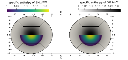
The SGRID code uses surface-fitted coordinates to reduce the Runge phenomenon at the surface of the star. Each time we update the specific enthalpy (step 5 in the iteration), we adapt the grid such that the boundaries of spectral elements coincide with the new surface of the outer fluid. That means we only construct configurations in which the surfaces of the two fluids do not intersect, which would in principle be possible given the different deformabilities of the fluids. Furthermore, we do not construct domains that are adapted to the surface of the inner fluid. Therefore, at the surface of the inner fluid one can expect to observe the Runge phenomenon and a slight degradation of the convergence in the truncation error. Fig. 1 shows a visualisation of the deformed spectral elements inside the NS and the distribution of matter in terms of the specific enthalpy, for a configuration with a DM particle mass of 170 MeV.
To close the system, the EoS is required to relate , , , and . For the EoS, SGRID reads in either parameters of piecewise polytropes or EoS tables. EoS tables are interpolated in a thermodynamically consistent manner [87] using a cubic Hermite interpolation. To find the thermodynamic quantities for a given specific enthalpy a Newton-Raphson root finder is used. At low densities we use a polytrope that is matched at the lowest density of the table.
We validated our implementation of the TOV equations and the EoS interpolation by comparison of the SGRID implementation and the code used in [11]. We find that the TOV-like solutions of the two implementations deviate only by machine round-off.
IV Results
IV.1 Parameters of Constructed Configurations
| ID | DM structure | |||||||
|---|---|---|---|---|---|---|---|---|
| 1 | 1.27300 | 0.0 | 1.27300 | 6.4 (9.5) | ||||
| 2 | 170 | 1.26641 | 1.27316 | 6.4 (9.5) | halo | |||
| 3 | 250 | 1.26590 | 1.27271 | 6.4 (9.5) | core | |||
| 4 | 350 | 1.26557 | 1.27243 | 6.4 (9.5) | core | |||
| 5 | 500 | 1.26534 | 1.27225 | 6.4 (9.5) | core | |||
| 6 | 750 | 1.26518 | 1.27212 | 6.4 (9.5) | core | |||
| 7 | 1000 | 1.26511 | 1.27207 | 6.4 (9.5) | core | |||
| 8 | 350 | 1.20503 | 1.27271 | 6.2 (9.2) | halo | |||
| 9 | 500 | 1.20056 | 1.26883 | 6.2 (9.2) | core | |||
| 10 | 750 | 1.19713 | 1.26590 | 6.1 (9.0) | core | |||
| 11 | 1000 | 1.19552 | 1.26450 | 6.1 (9.0) | core |
We consider different configurations by varying DM particle mass, mass fraction of DM and separation between NSs. In all configurations the individual NSs have the same total rest mass, i. e., the combined rest mass of BM and DM is . In all setups, the NSs have equal masses and are irrotational, , i. e., they are non-spinning. The assumption of vanishing spin is reasonable, because NSs spin down, e. g. due to magnetic breaking, and the NSs in binary mergers are usually very old, i. e. they have spun down for a long time.
We select six values of the DM particle mass in the range between 170 MeV and 1000 MeV, i.e., 170, 250, 350, 550, 750, and 1000 MeV. Furthermore we consider configurations with a DM rest mass fraction of 0%, 0.5% and 5%. In Table 2 we give an overview of the different configurations and report the properties a corresponding isolated NSs would have. There we also show the gravitational masses defined as
| (21) |
with the radius of the surface of fluid. In a binary system the gravitational mass of an individual NS can only be defined in a meaningful way in the limit of infinite separation, in which the binary components can be viewed as isolated. Hence we chose to work with fixed baryonic rest masses instead, which is invariantly defined even in binary systems.
The choice of the lowest DM particle mass value, 170 MeV, is motivated by the results of Ref. [11], where it was shown that for the DM particle masses below 174 MeV DM admixed NSs agree with astrophysical observations of the heaviest NSs for an arbitrary relative fraction of DM. Note, that this is not the case for the higher particle mass, where the fraction of DM is constrained in some interval (for more details see Ref. [11]). Moreover, the chosen mass of 170 MeV and the fraction of 0.5% leads to a relatively small halo of approximately twice the radius of the BM component, which is easy to model. When the size of the halos overlap, it is no longer possible to fit the element surfaces to the outer fluid of a star. Hence, we are discarding the configurations of DM particles with DM particle masses of 170 MeV and 250 MeV in the 5.0% DM case. Fermionic DM particles with a mass of 1000 MeV present an interesting case, that resembles nucleons.
We focus on three particular configurations on the extreme opposite of our parameter spectrum. Configuration 2 has the smallest DM particle mass, , and the smallest non-vanishing DM fraction, 0.5%. In this configuration the DM extends beyond the surface of the baryonic fluid and in figures we consequently label it as the dark halo configuration. On the other side of the spectrum we find configuration 2 with the largest DM particle mass, , and a DM fraction of 5%, for which the DM is concentrated in the core of the stars. Consequently we label the latter as the dark core configuration. We note however, that the name dark halo does not indicate that DM exists only in the surroundings of the star. In fact most of the DM is still concentrated in the center as can be appreciated from Fig. 1. In the same way the core of the dark core configuration includes a mixture of BM and DM. The third configuration is the special case of a purely baryonic star, the single fluid configuration (ID 2), which we use as a reference.
We describe BM by a piecewise-polytropic fit [54] to the SLy EoS [55]. As a model of DM, we investigate the degenerate, relativistic Fermi gas of spin- particles at zero temperature, for which the EoS is read in as tabulated data. EoSs at zero temperature are sufficient for our calculations, because the Fermi energy of the system is much higher than its temperature. The typical temperature of NS cores is of the order of K [88, 89]. We assume that DM has the same temperature as the BM, because the captured DM particles keep scattering with baryons, rarely but often enough to thermalise with the BM component. A core temperature of approximately K is much lower than the Fermi energy of BM. This is also true for the Fermi gas EoS we consider, e. g. in the dark halo case the Fermi energy of DM reaches 403 MeV in the center of the star, an energy smaller than that of the BM, but still much larger than the temperature of the star, MeV. In evolutions the neutron stars heat up when they collide, so that it would become necessary to use finite temperature EoSs. This can be achieved by employing EoS tabulated at finite temperatures, e. g. the finite-temperature SLy EoS of [90, 91], or by adding a temperature dependent term to the pressure [92].
IV.2 Convergence
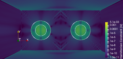
To validate the code, we check the convergence of the Hamiltonian constraint for a dark halo configuration of NSs with a separation of 44 (65.0 km) on a quasi-circular orbit.
Fig. 2 shows the magnitude of the Hamiltonian constraint on the plane. The constraint violations are largest in the interior of the star, where they reach values up to , whereas in the vacuum regions the error drops to values below , but with some spikes on the order of at the element boundaries, which is a behaviour commonly seen for spectral codes, an example being Fig. 10 of [69]. Such spikes in the Hamiltonian constraint usually do not cause any problems in subsequent evolutions. Furthermore the magnitude of these spikes converges towards zero with increasing resolution.
The Hamiltonian constraint is largest in the region where the inner fluid is non-vanishing. In Fig. 2 one can observe a clear transition on the surface of the baryonic fluid to lower constraint violations in the DM halo.
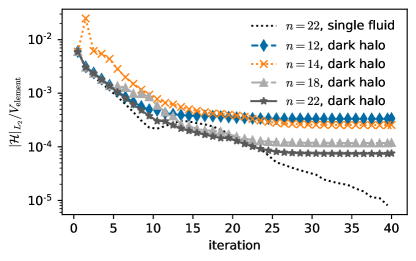
Fig. 3 demonstrates the development of the volume-normalised -norm of the Hamiltonian constraint for the inner cube of one of the stars during the iterative solving process. The figure shows the behaviour for different number of points in each dimension, which is the same for each spectral element. All curves show a saturation in the norm of the Hamiltonian constraint towards the end of the iteration process, which for all configurations is stopped after 40 iterations. Furthermore, it is visible that higher resolution leads to smaller violations of the Hamiltonian constraint in the final solution. For comparison Fig. 3 also shows the sequence for a corresponding single fluid configuration with the same mass and separation. After 40 iterations the single fluid configuration has a Hamiltonian constraint 10 smaller than the dark halo configurations and it does not show any signs of saturation, i. e. it would probably reach even smaller constraint violations if iterated further. The reason for this discrepancy is the position of the boundary of the BM, which in the dark halo case lies in the interior of the spectral element instead of the element surface and therefore due to Gibbs’ phenomenon requires more resolution to reach the same constraint violations. To improve the efficiency of the method it would be possible to introduce an advanced domain decomposition with surface adapted coordinates for the inner and outer fluid.
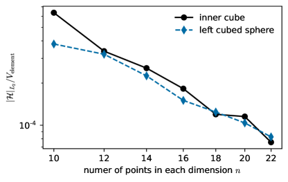
The convergence in the final solution is further investigated in Fig. 4, which shows its -norm of the Hamiltonian constraint with respect to the number of collocation points in the spectral elements. The figure shows the constraint violation for the inner cube element and for the cubed sphere facing towards the companion star, which is also representative for all other cubed sphere elements inside the NSs. The curves are almost straight lines on the log-log-plot of Fig. 4, which is compatible with a polynomial convergence of the constraints, i. e., , with the order of convergence. This is the expected convergence behaviour for non-smooth data, which we have due to the surface of the inner fluid. Using the highest and lowest resolution we can estimate the order of convergence in the inner cube element to be .
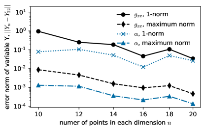
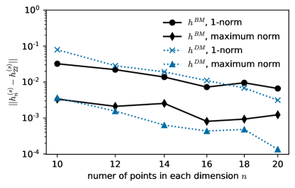
To investigate the convergence of the actual solution variables we interpolate the data from different resolutions on a common set of points and compute norms of the estimated errors on these points. We interpolate the solution onto a -grid equidistant in each direction, with coordinate components given by . This grid includes some points with pure vacuum, points with only one fluid present and points with both fluids present. The error in the solution is estimated by taking the difference to the solution with the highest resolution, i. e., the solution that has 22 points in each dimension of the spectral elements. In Fig. 5 we show the convergence of the 1-norm and the maximum norm over the set of interpolated points for the component of the metric and the lapse . Both quantities do not show a monotonic decay of the error, but there is an overall trend of decaying error. This somewhat broken convergence behaviour can again be attributed to the presence of non-smooth fields on the surface of the inner fluid. Fig. 6 shows the convergence of the error in the specific enthalpy. The DM in this configuration is fitted to the element boundaries and its specific enthalpy displays a relatively clear convergence behaviour. The BM fluid on the other hand shows a very broken convergence and only very little improvement from the lowest to the highest number of points. The maximum norm of the error is actually growing for the two largest number of points, whereas the 1-norm of the error is also slightly broken, but with an overall behaviour similar to that of and .
It should be noted, that it is not clear whether the formalisms used to construct NS binary initial data actually possesses a unique solution and likewise this is true for our formalism in Sec. II. The partial differential equation (12) is not strictly elliptic on the fluid surface and hence the standard theorems for the uniqueness of the solution can not be applied. Instead our algorithm might find a solution of many possible, which is another possible explanation for the slightly broken convergence behaviour.
IV.3 Difference in the Fluid Velocities
It is worth pointing out that even if the BM and DM fluid components are both irrotational, i. e., non-spinning, the exact velocity profiles are not the same. The reason for this does not lie in the notion of an irrotational fluid, but is caused by differences in the fluids’ equations of motion. An irrotational fluid [93, 81, 34] is defined by the vanishing of its kinematic vorticity tensor [94]
| (22) |
with and its rotational component, in Eq. 7, vanishes. This notion does not depend on the thermodynamic properties of the fluid and hence differences in the velocities can only be the result of the of the equations of motion used in the derivation of the formlalism in Sec. II, i. e. the Euler equations [93, 81, 34]
| (23) |
which follow from , and the continuity equation
| (24) |
If for example the DM would have the same four-velocity as the BM, it would still be irrotational, but might be incompatible with the laws of energy-momentum or particle number conservation.
In nature the disparity in the fluid velocities is affected by two counter-acting effects, particle scattering between BM and DM on the one hand and physics determining spin-down on the other hand. In our formulation the two fluids are modelled as non-interacting, but the BM-DM scattering cross-section might be non-zero in nature, which would drive the two fluids towards a common velocity. This process is counter-acted by effects driving the fluid into an irrotational state, as for example magnetic braking for BM [95, 96, 97]. It is unclear whether a similar effect exists for DM and whether it is dominant over the effect of BM-DM scattering. By assuming vanishing of the kinematic vorticity for the DM component, we assume that such an effect exists and it is also dominating over the scattering with BM.
We find that both fluids move with basically the same velocity, with coinciding velocities in the star center, but increasing difference towards the surface of the inner fluid. We quantify this effect in terms of the residual three-velocity , in which the orbital movement given by the Killing vector is split off,
| (25) |
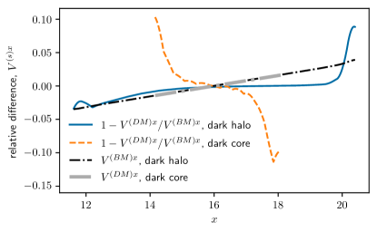
Fig. 7 shows the -component of and the relative difference of the fluid velocities for the region in which both fluids are present. We present results for configurations at a separation of 32 , a separation at which the DM halos in the dark halo configurations (ID 2) are already relatively close and deformed, as we demonstrate in Fig. 1. We find that differences in the two fluids are smaller for larger separation, which is intuitively understandable, because for large separations the system goes to the limit of isolated NSs in which the fluid velocities coincide.
The data in Fig. 7 is shown along a diagonal through the star parametrized in the following way: , where is the center of the star. We choose to present the data along this diagonal because the difference has a quadrupolar structure with nodes going through and being approximately parallel to the - and -axes. Hence the difference is basically zero on the - and -axes, but very prominent along the specified diagonal. The relative difference between the residual velocities is below 0.2% near the center of the star and reaches up to 10% on the surfaces of the inner fluids. The difference between the velocities of the dark halo (ID 2) and dark core (ID 2) configurations is relatively small, which can be seen from the fact the curves of the velocities of the inner fluids lie on top of each other.
IV.4 Binding Energy
NSs with a DM component are more tightly bound, because the DM component adds gravitating mass, but provides no additional repulsion to balance the gravitational pressure. This effect is well studied and was already demonstrated by several authors [11, 4, 98]. In the following we investigate the effect of DM on the energetics of the binary system, i. e. the orbital binding energy.
The gravitational binding energy of the particles is the difference of the ADM mass [99, 33, 34] and the sum of the rest masses of the components. If all fluid particles would fall in from infinity, the true ADM mass would equal the total rest mass. However, the configurations that we construct do not contain GWs and therefore they do not model the energy lost in gravitational radiation. The difference in our ADM mass estimate and the total rest mass is, therefore, a measure of the particle binding energy:
| (26) |
We have constructed the configurations with fixed baryonic masses, but configurations with different separation distance between the stars or particle mass will have a different ADM mass, similar to how the isolated stars in Table 2 have different gravitational masses. To make the results comparable in the figures we show quantities appropriately rescaled by .
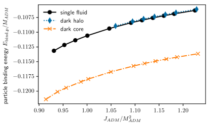
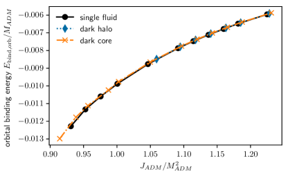
We construct a series of configurations with varying orbital separation . The orbital frequency changes as well, since it is a function of the masses and the orbital separation. Fig. 8 shows the rescaled particle binding energy as a function of our estimate for the ADM angular momentum . It can be seen that dark core configurations (ID 2) are more tightly bound than single fluid configurations. The dark halo configurations (ID 2) seemingly coincide with the single fluid case. This can be attributed to the relatively low DM fraction of only 0.5% in these configurations. All configurations are more tightly bound for smaller corresponding to smaller stellar separations. This is due to the stronger orbital binding between the two stars.
Most of the binding energy is contained in the individual stars and the contribution of the orbital binding energy is universal in all configurations. The orbital binding energy is the energy necessary for the two NSs to escape to infinity. It can be computed using the gravitational mass of the components, by
| (27) |
The gravitational masses are obtained by solving a TOV-like equation for isolated stars that have the same rest masses. The gravitational mass is smaller than the rest mass , because it accounts for the binding energy. Hence, contains only contributions of the binding energy that are due to the mutual binding between the stars. Fig. 9 shows that the relation between orbital binding energy and ADM angular momentum (both appropriately rescaled by ) is mostly independent of the DM configuration as the lines are falling on top of each other.
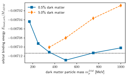
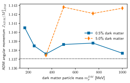
To investigate the small effect of the particle mass, we construct configurations at a range of DM particle masses from 170 MeV to 1000 MeV at a fixed binary separation of 36 (53.2 km) Fig. 10 shows the orbital binding energy for the case of 0.5% and 5% of DM. For the case of 0.5% DM (IDs 2 to 2) we find that the orbital binding energy has a minimum around 550 MeV. The value of the minimum lies even below that of the corresponding single fluid configuration. For the case of 5% of DM (IDs 2 to 2) we do not observe a minimum, but an orbital energy always larger than in the corresponding single fluid configuration and increase roughly linear with . We emphasise that for this comparison one has to keep in mind that configurations with different also have different angular momentum. However, as is shown in Fig. 11 the variation in the rescaled ADM angular momentum is below 1%. We also find no clear relation between the ADM angular momentum and , but we find that larger amounts of DM tend to lead to larger angular momentum.
Figures 10 and 11 also demonstrate that by decreasing the amount of DM the configurations reach the single fluid limit. In almost all cases the configurations with lower DM fraction have a binding energy and angular momentum that is closer to that of the single fluid case. Only for the particle masses of 350 MeV the angular momentum of the 5.0% configuration is closer to the single fluid limit. However, it must be noted that for this case the DM forms a halo around the BM and therefore this configuration is not representative for the limit of low DM content.
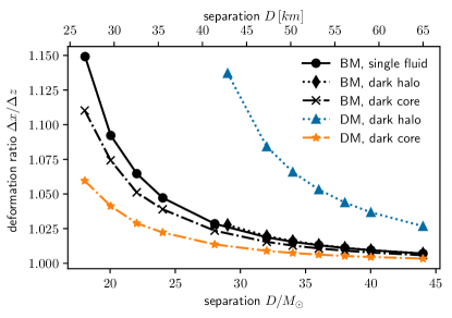
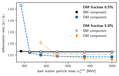
IV.5 Deformation
To quantify the deformation of the stars we compute the ratio of the diameters along the orbital radius and along the polar axes. The diameter along the orbital radius is taken as , largest difference in the -coordinates of two points on the fluid surface. The polar diameter , is the largest difference in the -coordinate of two points on the fluid surface. The tidal force of the companion stretches the star in -direction, whereas the poles are slightly flattened. This measure of deformation is of course coordinate-dependent, but it still provides some physical insights.
We analyse the same set of configurations with varying orbital separation as in the previous section. Fig. 12 shows the deformation for each fluid surface. When the NSs are closer, the tidal forces on the companion are stronger and hence the deformation is stronger. It can be observed that NSs with a DM core are systematically less deformed than their one-fluid counterparts.
The strong deformation in the dark halo case (ID 2) can also be seen in Fig. 1, which shows a cut through the plane. For a separation of 32 (47.3 km) the deformation is clearly visible by eye. At a separation of 28 (41.3 km) the deformation becomes already so strong that the surfaces of the NSs touch and mass shedding occurs.
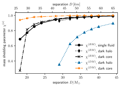
The closeness to mass shedding can be quantified in terms of the mass-shedding parameter , which was first introduced in [71] and which we define as
| (28) |
where the label “eq” denotes the point on the surface, which is facing towards the companion star and for which the -coordinate is extremal. The label “pole” denotes the surface points at which the -coordinate is extremal and where in Eq. (28) the label “avg” indicates that we have averaged over the values at the “north and south pole”. Note that for non-spinning stars the “north” and “south pole” values only differ slightly due to round-off error. In the mass shedding limit will tend to 0. We evaluate the for each fluid component individually on the respective fluid surfaces. We show the resulting as a function of the distance of the centres of the stars in Fig. 13. The DM fluid in the dark halo scenario (ID 2) is easily deformable, which leads to a relatively small mass shedding parameter of 0.9 already at a separation of 44 . We find that a separation of 28 leads to a configuration with touching star surfaces, from which we conclude that mass shedding occurs somewhere at a separation between 28 and 29 , which means the system will transition relatively slowly to the mass shedding regime over a time where the two NSs decrease their separation by 16 . For the dark core configurations (ID 2), on the other hand, the transition to mass shedding is rather sudden with reaching a value of 0.9 at separation of approximately 23 and the mass shedding occurring for the baryonic fluid at a separation of 16 .
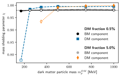
In Figs. 14 and 15 we show the deformation and mass shedding parameters as functions of the DM particle mass corresponding to all configurations in Table 2 and for a fixed binary separation of 36 (53.2 km). For the case of 0.5% DM the BM deformation as well as have practically the same value as in the single fluid case. For 5% of DM the BM deformation is smaller and is larger owing to the higher compactness in these configurations. The DM fluid is less strongly deformed when is large. In particular when the DM fluid changes character from being the halo to being the core component, the deformation decreases rapidly and increases rapidly.
V Conclusion
We have extended the SGRID code to construct constraint-solved, quasi-equlibrium configurations of binaries of NSs consisting of two non-interacting fluids. The second fluid represents DM that can comprise some part of the matter of NS. In this study we have used the EoS of a degenerate, relativistic Fermi gas with different particle masses to model the DM fluid. These quasi-equlibrium configurations can be used as initial data for NR inspiral simulations of DM admixed NS binaries. The BAM code can already evolve mirror DM [100] and could be easily extended to allow for general EoS for the DM fluid.
Another possible application of the two fluid approach are superfluid NS cores. At sufficiently high density BM forms a state made of superfluid neutrons and superconducting protons, which can be described in a two fluid approach. However, the two fluids still interact with each other due to the entrainment effect and the condition of beta-equilibrium [101]. The evolution equations for interacting multifluid systems have been discussed in [30, 31], but so far no formalism exists for the construction of initial data for NS binary systems. For the construction of such initial data the formalism in this work could be extended using an interaction model similar to the one used in solutions of isolated NS with superfluid cores [102, 103] and taking into account mutual friction [104]. In binary NS collisions the temperature will rise above the critical temperature for superfluidity and superconductivity. The case of finite temperature superfluid dynamics was discussed in [105].
We have tested the convergence of the constructed configurations with respect to resolution. The Hamiltonian constraint converges polynomially with an order of . The lack of exponential convergence can be attributed to the presence of the non-smooth transition of the density at the surface of the inner fluid, which is not fitted to the boundaries of the spectral elements. Self-convergence tests for metric components and the specific enthalpies show that the solution improves with increasing resolution, but with a slightly broken convergence towards higher resolution, which we again attribute to the surface of the inner fluid. For future improvements to the code it is a worthwhile consideration to implement a new grid layout that allows fitting to the surface of a second fluid
We have shown that the two fluids do not have the exact same velocities, but that the difference in the residual velocities reaches up to 10% on the surface of the inner fluids. The difference in the velocity profiles will be even stronger if one assumes independent rotational states for the components. In this work we only investigated only purely irrotational configurations, but our formalism, in principle, allows to construct configurations with arbitrary spin for the individual stars and fluid components. This is relevant in particular for the DM component, which might only have insufficient mechanisms to lose angular momentum and hence could be in a state of rapid rotation.
The presence of DM affects the compactness and deformability of NSs, which will change the merger dynamics. We have shown that the presence of DM can delay the point of mass-shedding to a later stage of the inspiral, i. e., towards closer separations. This is in accordance with the findings in numerical evolutions of two-fluid binary mergers [100]. In the case of a DM halo, mass shedding could occur much earlier than for the baryonic component. However the matter contained in the DM halo is rather low and hence the impact of DM mass shedding on the dynamics of the BM is potentially small, nevertheless, dynamical simulations are needed to verify this assumption.
Acknowledgements.
This work was supported by funding from the FCT – Fundação para a Ciência e a Tecnologia, I.P., within the Project No. EXPL/FIS-AST/0735/2021. H.R.R. and V.S. also acknowledge the support from the project No. UIDB/04564/2020, and UIDP/04564/2020. W.T. acknowledges funding from the National Science Foundation under grant PHY-2136036.References
- Goldman and Nussinov [1989] I. Goldman and S. Nussinov, Weakly Interacting Massive Particles and Neutron Stars, Phys. Rev. D 40, 3221 (1989).
- Narain et al. [2006] G. Narain, J. Schaffner-Bielich, and I. N. Mishustin, Compact stars made of fermionic dark matter, Phys. Rev. D 74, 063003 (2006), arXiv:astro-ph/0605724 [astro-ph] .
- Ciarcelluti and Sandin [2011] P. Ciarcelluti and F. Sandin, Have neutron stars a dark matter core?, Phys. Lett. B 695, 19 (2011), arXiv:1005.0857 [astro-ph.HE] .
- Leung et al. [2011] S. C. Leung, M. C. Chu, and L. M. Lin, Dark-matter admixed neutron stars, Phys. Rev. D 84, 107301 (2011), arXiv:1111.1787 [astro-ph.CO] .
- Leung et al. [2012] S. C. Leung, M. C. Chu, and L. M. Lin, Equilibrium Structure and Radial Oscillations of Dark Matter Admixed Neutron Stars, Phys. Rev. D 85, 103528 (2012), arXiv:1205.1909 [astro-ph.CO] .
- Zurek [2014] K. M. Zurek, Asymmetric Dark Matter: Theories, Signatures, and Constraints, Phys. Rept. 537, 91 (2014), arXiv:1308.0338 [hep-ph] .
- Goldman et al. [2013] I. Goldman, R. N. Mohapatra, S. Nussinov, D. Rosenbaum, and V. Teplitz, Possible Implications of Asymmetric Fermionic Dark Matter for Neutron Stars, Phys. Lett. B 725, 200 (2013), arXiv:1305.6908 [astro-ph.CO] .
- Gresham et al. [2017] M. I. Gresham, H. K. Lou, and K. M. Zurek, Nuclear Structure of Bound States of Asymmetric Dark Matter, Phys. Rev. D 96, 096012 (2017), arXiv:1707.02313 [hep-ph] .
- Ellis et al. [2018a] J. Ellis, G. Hütsi, K. Kannike, L. Marzola, M. Raidal, and V. Vaskonen, Dark matter effects on neutron star properties, Phys. Rev. D 97, 123007 (2018a), arXiv:1804.01418 [astro-ph.CO] .
- Nelson et al. [2019] A. E. Nelson, S. Reddy, and D. Zhou, Dark halos around neutron stars and gravitational waves, J. Cosm. Astrop. Phys. 2019, 012 (2019), arXiv:1803.03266 [hep-ph] .
- Ivanytskyi et al. [2020] O. Ivanytskyi, V. Sagun, and I. Lopes, Neutron stars: New constraints on asymmetric dark matter, Phys. Rev. D 102, 063028 (2020), arXiv:1910.09925 [astro-ph.HE] .
- Das et al. [2020a] H. C. Das, A. Kumar, B. Kumar, S. K. Biswal, T. Nakatsukasa, A. Li, and S. K. Patra, Effects of dark matter on the nuclear and neutron star matter, Mon. Not. R. Astron. Soc. 495, 4893 (2020a), arXiv:2002.00594 [nucl-th] .
- Das et al. [2020b] A. Das, T. Malik, and A. C. Nayak, Dark matter admixed neutron star properties in the light of gravitational wave observations: a two fluid approach (2020b), arXiv:2011.01318 [nucl-th] .
- Sagun et al. [2022a] V. Sagun, E. Giangrandi, O. Ivanytskyi, I. Lopes, and K. A. Bugaev, Constraints on the fermionic dark matter from observations of neutron stars, PoS PANIC2021, 313 (2022a), arXiv:2111.13289 [astro-ph.HE] .
- Di Giovanni et al. [2022] F. Di Giovanni, N. Sanchis-Gual, P. Cerdá-Durán, and J. A. Font, Can fermion-boson stars reconcile multimessenger observations of compact stars?, Phys. Rev. D 105, 063005 (2022), arXiv:2110.11997 [gr-qc] .
- Rafiei Karkevandi et al. [2021] D. Rafiei Karkevandi, S. Shakeri, V. Sagun, and O. Ivanytskyi, Tidal deformability as a probe of dark matter in neutron stars, in 16th Marcel Grossmann Meeting on Recent Developments in Theoretical and Experimental General Relativity, Astrophysics and Relativistic Field Theories (2021) arXiv:2112.14231 [astro-ph.HE] .
- Leung et al. [2022] K.-L. Leung, M.-c. Chu, and L.-M. Lin, Tidal deformability of dark matter admixed neutron stars, Phys. Rev. D 105, 123010 (2022), arXiv:2207.02433 [astro-ph.HE] .
- Rafiei Karkevandi et al. [2022] D. Rafiei Karkevandi, S. Shakeri, V. Sagun, and O. Ivanytskyi, Bosonic dark matter in neutron stars and its effect on gravitational wave signal, Phys. Rev. D 105, 023001 (2022), arXiv:2109.03801 [astro-ph.HE] .
- Sagun et al. [2022b] V. Sagun, E. Giangrandi, O. Ivanytskyi, C. Providência, and T. Dietrich, How does dark matter affect compact star properties and high density constraints of strongly interacting matter, 15th Conference on Quark Confinement and the Hadron Spectrum, EPJ Web of Conferences 274, 07009 (2022b), arXiv:2211.10510 [astro-ph.HE] .
- Shakeri and Karkevandi [2022] S. Shakeri and D. R. Karkevandi, Bosonic Dark Matter in Light of the NICER Precise Mass-Radius Measurements (2022), arXiv:2210.17308 [astro-ph.HE] .
- Maselli et al. [2017] A. Maselli, P. Pnigouras, N. G. Nielsen, C. Kouvaris, and K. D. Kokkotas, Dark stars: gravitational and electromagnetic observables, Phys. Rev. D 96, 023005 (2017), arXiv:1704.07286 [astro-ph.HE] .
- Giangrandi et al. [2023] E. Giangrandi, V. Sagun, O. Ivanytskyi, C. Providência, and T. Dietrich, The effects of self-interacting bosonic dark matter on neutron star properties, The Astrophysical Journal 953, 115 (2023), arXiv:2209.10905 [astro-ph.HE] .
- Rutherford et al. [2023] N. Rutherford, G. Raaijmakers, C. Prescod-Weinstein, and A. Watts, Constraining bosonic asymmetric dark matter with neutron star mass-radius measurements, Phys. Rev. D 107, 103051 (2023), arXiv:2208.03282 [astro-ph.HE] .
- Bamber et al. [2023] J. Bamber, J. C. Aurrekoetxea, K. Clough, and P. G. Ferreira, Black hole merger simulations in wave dark matter environments, Phys. Rev. D 107, 024035 (2023), arXiv:2210.09254 [gr-qc] .
- Cole et al. [2022] P. S. Cole, G. Bertone, A. Coogan, D. Gaggero, T. Karydas, B. J. Kavanagh, T. F. M. Spieksma, and G. M. Tomaselli, Disks, spikes, and clouds: distinguishing environmental effects on BBH gravitational waveforms (2022), arXiv:2211.01362 [gr-qc] .
- Ellis et al. [2018b] J. Ellis, A. Hektor, G. Hütsi, K. Kannike, L. Marzola, M. Raidal, and V. Vaskonen, Search for Dark Matter Effects on Gravitational Signals from Neutron Star Mergers, Phys. Lett. B 781, 607 (2018b), arXiv:1710.05540 [astro-ph.CO] .
- Bezares et al. [2019] M. Bezares, D. Viganò, and C. Palenzuela, Gravitational wave signatures of dark matter cores in binary neutron star mergers by using numerical simulations, Phys. Rev. D 100, 044049 (2019), arXiv:1905.08551 [gr-qc] .
- Bauswein et al. [2020] A. Bauswein, G. Guo, J.-H. Lien, Y.-H. Lin, and M.-R. Wu, Compact Dark Objects in Neutron Star Mergers (2020), arXiv:2012.11908 [astro-ph.HE] .
- Hippert et al. [2023] M. Hippert, E. Dillingham, H. Tan, D. Curtin, J. Noronha-Hostler, and N. Yunes, Dark matter or regular matter in neutron stars? how to tell the difference from the coalescence of compact objects, Phys. Rev. D 107, 115028 (2023), arXiv:2211.08590 [astro-ph.HE] .
- Andersson and Comer [2021] N. Andersson and G. L. Comer, Relativistic fluid dynamics: physics for many different scales, Living Reviews in Relativity 24, 1 (2021), arXiv:2008.12069 [gr-qc] .
- Andersson [2021] N. Andersson, A multifluid perspective on multimessenger modelling (2021), arXiv:2103.10220 [gr-qc] .
- Emma et al. [2022a] M. Emma, F. Schianchi, F. Pannarale, V. Sagun, and T. Dietrich, Numerical simulations of dark matter admixed neutron star binaries (2022a), arXiv:2206.10887 [gr-qc] .
- Gourgoulhon [2012] E. Gourgoulhon, 3+1 Formalism in General Relativity (Springer, Berlin, 2012) gr-qc/0703035 .
- Baumgarte and Shapiro [2010] T. W. Baumgarte and S. L. Shapiro, Numerical Relativity: Solving Einstein’s Equations on the Computer (Cambridge University Press, Cambridge, 2010).
- Tichy [2017] W. Tichy, The initial value problem as it relates to numerical relativity, Rept. Prog. Phys. 80, 026901 (2017), arXiv:1610.03805 [gr-qc] .
- Tolman [1939] R. C. Tolman, Static solutions of Einstein’s field equations for spheres of fluid, Phys. Rev. 55, 364 (1939).
- Oppenheimer and Volkoff [1939] J. R. Oppenheimer and G. M. Volkoff, On massive neutron cores, Phys. Rev. 55, 374 (1939).
- Kouvaris [2013] C. Kouvaris, The Dark Side of Neutron Stars, Adv. High Energy Phys. 2013, 856196 (2013), arXiv:1308.3222 [astro-ph.HE] .
- Bell et al. [2020] N. F. Bell, G. Busoni, S. Robles, and M. Virgato, Improved Treatment of Dark Matter Capture in Neutron Stars, Journal of Cosmology and Astroparticle Physics 2020 (09), 028, arXiv:2004.14888 [hep-ph] .
- Bell et al. [2021] N. F. Bell, G. Busoni, T. F. Motta, S. Robles, A. W. Thomas, and M. Virgato, Nucleon Structure and Strong Interactions in Dark Matter Capture in Neutron Stars, Phys. Rev. Lett. 127, 111803 (2021), arXiv:2012.08918 [hep-ph] .
- Kouvaris and Tinyakov [2010] C. Kouvaris and P. Tinyakov, Can neutron stars constrain dark matter?, Phys. Rev. D 82, 063531 (2010), arXiv:1004.0586 [astro-ph.GA] .
- Del Popolo et al. [2020] A. Del Popolo, M. Le Delliou, and M. Deliyergiyev, Neutron Stars and Dark Matter, Universe 6, 222 (2020).
- Nguyen and Tait [2023] T. T. Q. Nguyen and T. M. P. Tait, Bounds on long-lived dark matter mediators from neutron stars, Phys. Rev. D 107, 115016 (2023), arXiv:2212.12547 [hep-ph] .
- Bertone and Fairbairn [2008] G. Bertone and M. Fairbairn, Compact Stars as Dark Matter Probes, Phys. Rev. D 77, 043515 (2008), arXiv:0709.1485 [astro-ph] .
- Baryakhtar et al. [2022] M. Baryakhtar et al., Dark Matter In Extreme Astrophysical Environments, in 2022 Snowmass Summer Study (2022) arXiv:2203.07984 [hep-ph] .
- Kouvaris [2008] C. Kouvaris, Wimp annihilation and cooling of neutron stars, Phys. Rev. D 77, 023006 (2008), arXiv:0708.2362 [astro-ph] .
- de Lavallaz and Fairbairn [2010] A. de Lavallaz and M. Fairbairn, Neutron stars as dark matter probes, Phys. Rev. D 81, 123521 (2010), arXiv:1004.0629 [astro-ph.GA] .
- Hamaguchi et al. [2019] K. Hamaguchi, N. Nagata, and K. Yanagi, Dark Matter Heating vs. Rotochemical Heating in Old Neutron Stars, Phys. Lett. B 795, 484 (2019), arXiv:1905.02991 [hep-ph] .
- Pérez-García and Silk [2012] M. Á. Pérez-García and J. Silk, Dark matter seeding and the kinematics and rotation of neutron stars, Phys. Lett. B 711, 6 (2012), arXiv:1111.2275 [astro-ph.CO] .
- Sedrakian [2016] A. Sedrakian, Axion cooling of neutron stars, Phys. Rev. D 93, 065044 (2016), arXiv:1512.07828 [astro-ph.HE] .
- Sedrakian [2019] A. Sedrakian, Axion cooling of neutron stars. II. Beyond hadronic axions, Phys. Rev. D 99, 043011 (2019), arXiv:1810.00190 [astro-ph.HE] .
- Dietrich and Clough [2019] T. Dietrich and K. Clough, Cooling binary neutron star remnants via nucleon-nucleon-axion bremsstrahlung, Phys. Rev. D 100, 083005 (2019), arXiv:1909.01278 [gr-qc] .
- Buschmann et al. [2022] M. Buschmann, C. Dessert, J. W. Foster, A. J. Long, and B. R. Safdi, Upper Limit on the QCD Axion Mass from Isolated Neutron Star Cooling, Phys. Rev. Lett. 128, 091102 (2022), arXiv:2111.09892 [hep-ph] .
- Read et al. [2009] J. S. Read, B. D. Lackey, B. J. Owen, and J. L. Friedman, Constraints on a phenomenologically parameterized neutron-star equation of state, Phys. Rev. D 79, 124032 (2009), arXiv:0812.2163 [astro-ph] .
- Douchin and Haensel [2001] F. Douchin and P. Haensel, A unified equation of state of dense matter and neutron star structure, Astron. Astrophys. 380, 151 (2001), arXiv:astro-ph/0111092 .
- Antoniadis et al. [2013] J. Antoniadis, P. C. C. Freire, N. Wex, T. M. Tauris, R. S. Lynch, M. H. van Kerkwijk, M. Kramer, C. Bassa, V. S. Dhillon, T. Driebe, J. W. T. Hessels, V. M. Kaspi, V. I. Kondratiev, N. Langer, T. R. Marsh, M. A. McLaughlin, T. T. Pennucci, S. M. Ransom, I. H. Stairs, J. van Leeuwen, J. P. W. Verbiest, and D. G. Whelan, A Massive Pulsar in a Compact Relativistic Binary, Science 340, 448 (2013), arXiv:1304.6875 [astro-ph.HE] .
- Fonseca et al. [2021] E. Fonseca et al., Refined Mass and Geometric Measurements of the High-mass PSR J0740+6620, Astrophys. J. Lett. 915, L12 (2021), arXiv:2104.00880 [astro-ph.HE] .
- Miller et al. [2019] M. C. Miller, F. K. Lamb, A. J. Dittmann, S. Bogdanov, Z. Arzoumanian, K. C. Gendreau, S. Guillot, A. K. Harding, W. C. G. Ho, J. M. Lattimer, R. M. Ludlam, S. Mahmoodifar, S. M. Morsink, P. S. Ray, T. E. Strohmayer, K. S. Wood, T. Enoto, R. Foster, T. Okajima, G. Prigozhin, and Y. Soong, Psr j0030+0451 mass and radius from nicer data and implications for the properties of neutron star matter, The Astrophysical Journal 887, L24 (2019), arXiv:1912.05705 [astro-ph.HE] .
- Riley et al. [2019] T. E. Riley et al., A NICER View of PSR J0030+0451: Millisecond Pulsar Parameter Estimation, Astrophys. J. Lett. 887, L21 (2019), arXiv:1912.05702 [astro-ph.HE] .
- Raaijmakers et al. [2020] G. Raaijmakers et al., Constraining the dense matter equation of state with joint analysis of NICER and LIGO/Virgo measurements, Astrophys. J. Lett. 893, L21 (2020), arXiv:1912.11031 [astro-ph.HE] .
- Miller et al. [2021] M. C. Miller et al., The Radius of PSR J0740+6620 from NICER and XMM-Newton Data, Astrophys. J. Lett. 918, L28 (2021), arXiv:2105.06979 [astro-ph.HE] .
- Riley et al. [2021] T. E. Riley et al., A NICER View of the Massive Pulsar PSR J0740+6620 Informed by Radio Timing and XMM-Newton Spectroscopy, Astrophys. J. Lett. 918, L27 (2021), arXiv:2105.06980 [astro-ph.HE] .
- Abbott et al. [2019] B. P. Abbott et al. (LIGO Scientific, Virgo), Properties of the binary neutron star merger GW170817, Phys. Rev. X 9, 011001 (2019), arXiv:1805.11579 [gr-qc] .
- Abbott et al. [2020] B. P. Abbott et al. (LIGO Scientific, Virgo), GW190425: Observation of a Compact Binary Coalescence with Total Mass , Astrophys. J. Lett. 892, L3 (2020), arXiv:2001.01761 [astro-ph.HE] .
- Clowe et al. [2006] D. Clowe, M. Bradač, A. H. Gonzalez, M. Markevitch, S. W. Randall, C. Jones, and D. Zaritsky, A direct empirical proof of the existence of dark matter, The Astrophysical Journal 648, L109 (2006), astro-ph/0608407 .
- Randall et al. [2008] S. W. Randall, M. Markevitch, D. Clowe, A. H. Gonzalez, and M. Bradac, Constraints on the Self-Interaction Cross-Section of Dark Matter from Numerical Simulations of the Merging Galaxy Cluster 1E 0657-56, Astrophys. J. 679, 1173 (2008), arXiv:0704.0261 [astro-ph] .
- Billard et al. [2022] J. Billard et al., Direct detection of dark matter—APPEC committee report*, Rept. Prog. Phys. 85, 056201 (2022), arXiv:2104.07634 [hep-ex] .
- Tichy [2012] W. Tichy, Constructing quasi-equilibrium initial data for binary neutron stars with arbitrary spins, Phys. Rev. D 86, 064024 (2012), arXiv:1209.5336 [gr-qc] .
- Tichy et al. [2019] W. Tichy, A. Rashti, T. Dietrich, R. Dudi, and B. Brügmann, Constructing binary neutron star initial data with high spins, high compactnesses, and high mass ratios, Phys. Rev. D 100, 124046 (2019), arXiv:1910.09690 [gr-qc] .
- [70] E. Gourgoulhon, P. Grandclément, J.-A. Marck, J. Novak, and K. Taniguchi, http://www.lorene.obspm.fr.
- Gourgoulhon et al. [2001] E. Gourgoulhon, P. Grandclément, K. Taniguchi, J.-A. Marck, and S. Bonazzola, Quasiequilibrium sequences of synchronized and irrotational binary neutron stars in general relativity: Method and tests, Phys. Rev. D 63, 064029 (2001), arXiv:gr-qc/0007028 [gr-qc] .
- Tacik et al. [2015] N. Tacik, F. Foucart, H. P. Pfeiffer, R. Haas, S. Ossokine, J. Kaplan, C. Muhlberger, M. D. Duez, L. E. Kidder, M. A. Scheel, and B. Szilágyi, Binary neutron stars with arbitrary spins in numerical relativity, Phys. Rev. D 92, 124012 (2015), arXiv:1508.06986 [gr-qc] .
- [73] P. Grandclément, S. Auliac, H. Roussille, and L. J. Papenfort, https://kadath.obspm.fr/fuka/.
- Papenfort et al. [2021] L. J. Papenfort, S. D. Tootle, P. Grandclément, E. R. Most, and L. Rezzolla, New public code for initial data of unequal-mass, spinning compact-object binaries, Phys. Rev. D 104, 024057 (2021), arXiv:2103.09911 [gr-qc] .
- Rashti et al. [2022] A. Rashti, F. M. Fabbri, B. Brügmann, S. V. Chaurasia, T. Dietrich, M. Ujevic, and W. Tichy, New pseudospectral code for the construction of initial data, Phys. Rev. D 105, 104027 (2022), arXiv:2109.14511 [gr-qc] .
- Uryū and Tsokaros [2012] K. Uryū and A. Tsokaros, New code for equilibriums and quasiequilibrium initial data of compact objects, Phys.Rev. D85, 064014 (2012), arXiv:1108.3065 [gr-qc] .
- Tsokaros et al. [2015] A. Tsokaros, K. Uryū, and L. Rezzolla, A new code for quasi-equilibrium initial data of binary neutron stars: corotating, irrotational and slowly spinning systems, Phys. Rev. D 91, 104030 (2015), arXiv:1502.05674 [gr-qc] .
- Uryū et al. [2019] K. Uryū, S. Yoshida, E. Gourgoulhon, C. Markakis, K. Fujisawa, A. Tsokaros, K. Taniguchi, and Y. Eriguchi, New code for equilibriums and quasiequilibrium initial data of compact objects. iv. rotating relativistic stars with mixed poloidal and toroidal magnetic fields, Phys. Rev. D 100, 123019 (2019), arXiv:1906.10393 [gr-qc] .
- Wittman et al. [2018] D. Wittman, N. Golovich, and W. A. Dawson, The Mismeasure of Mergers: Revised Limits on Self-interacting Dark Matter in Merging Galaxy Clusters, Astrophys. J. 869, 104 (2018), arXiv:1701.05877 [astro-ph.CO] .
- Cook [2000] G. B. Cook, Initial data for numerical relativity, Living Reviews in Relativity 3, 10.12942/lrr-2000-5 (2000), arXiv:gr-qc/0007085 [gr-qc] .
- Tichy [2011] W. Tichy, Initial data for binary neutron stars with arbitrary spins, Phys. Rev. D 84, 024041 (2011), arXiv:1107.1440 [gr-qc] .
- Kiuchi et al. [2009] K. Kiuchi, Y. Sekiguchi, M. Shibata, and K. Taniguchi, Longterm general relativistic simulation of binary neutron stars collapsing to a black hole, Phys. Rev. D80, 064037 (2009), arXiv:0904.4551 [gr-qc] .
- Kyutoku et al. [2014] K. Kyutoku, M. Shibata, and K. Taniguchi, Reducing orbital eccentricity in initial data of binary neutron stars, Phys. Rev. D 90, 064006 (2014), arXiv:1405.6207 [gr-qc] .
- Schäfer and Wex [1993] G. Schäfer and N. Wex, Phys. Lett. A 174, 196 (1993).
- Tichy et al. [2003] W. Tichy, B. Brügmann, M. Campanelli, and P. Diener, Binary black hole initial data for numerical general relativity based on post-newtonian data, Phys. Rev. D 67, 064008 (2003), arXiv:gr-qc/0207011 [gr-qc] .
- Tichy and Brügmann [2004] W. Tichy and B. Brügmann, Quasi-equilibrium binary black hole sequences for puncture data derived from helical killing vector conditions, Phys. Rev. D 69, 024006 (2004), arXiv:gr-qc/0307027 [gr-qc] .
- Swesty [1996] F. Swesty, Thermodynamically consistent interpolation for equation of state tables, Journal of Computational Physics 127, 118 (1996).
- Cumming et al. [2017] A. Cumming, E. F. Brown, F. J. Fattoyev, C. J. Horowitz, D. Page, and S. Reddy, Lower limit on the heat capacity of the neutron star core, Phys. Rev. C 95, 025806 (2017), arXiv:1608.07532 [astro-ph.HE] .
- Page et al. [2006] D. Page, U. Geppert, and F. Weber, The Cooling of compact stars, Nucl. Phys. A 777, 497 (2006), arXiv:astro-ph/0508056 .
- Gulminelli and Raduta [2015] F. Gulminelli and A. R. Raduta, Unified treatment of subsaturation stellar matter at zero and finite temperature, Phys. Rev. C 92, 055803 (2015), arXiv:1504.04493 [nucl-th] .
- Raduta and Gulminelli [2019] A. Raduta and F. Gulminelli, Nuclear statistical equilibrium equation of state for core collapse, Nuclear Physics A 983, 252 (2019), EoS table available at: https://compose.obspm.fr/eos/123, arXiv:1807.06871 [nucl-th] .
- Bauswein et al. [2010] A. Bauswein, H.-T. Janka, and R. Oechslin, Testing approximations of thermal effects in neutron star merger simulations, Phys. Rev. D 82, 084043 (2010), arXiv:1006.3315 [astro-ph.SR] .
- Shibata [1998] M. Shibata, A relativistic formalism for computation of irrotational binary stars in quasi equilibrium states, Phys. Rev. D 58, 024012 (1998), arXiv:gr-qc/9803085 .
- Hawking and Ellis [1973] S. W. Hawking and G. F. R. Ellis, The Large Scale Structure of Space-Time (Cambridge University Press, Cambridge (UK), 1973).
- Ostriker and Gunn [1969] J. P. Ostriker and J. E. Gunn, On the Nature of Pulsars. I. Theory, Astrophys. J. 157, 1395 (1969).
- Colpi et al. [2001] M. Colpi, A. Possenti, S. Popov, and F. Pizzolato, Spin and magnetism in old neutron stars, in Physics of Neutron Star Interiors, edited by D. Blaschke, A. Sedrakian, and N. K. Glendenning (Springer Berlin Heidelberg, Berlin, Heidelberg, 2001) pp. 440–466, astro-ph/0012394 .
- Rogers and Safi-Harb [2016] A. Rogers and S. Safi-Harb, On the diversity of compact objects within supernova remnants – II. energy-loss mechanisms, Monthly Notices of the Royal Astronomical Society 465, 383 (2016), arXiv:1610.04685 [astro-ph.HE] .
- Xiang et al. [2014] Q.-F. Xiang, W.-Z. Jiang, D.-R. Zhang, and R.-Y. Yang, Effects of fermionic dark matter on properties of neutron stars, Phys. Rev. C 89, 025803 (2014), arXiv:1305.7354 [astro-ph.SR] .
- Arnowitt et al. [1962] R. Arnowitt, S. Deser, and C. W. Misner, The dynamics of general relativity, in Gravitation: An Introduction to Current Research, edited by L. Witten (Wiley, New York, 1962) pp. 227–265.
- Emma et al. [2022b] M. Emma, F. Schianchi, F. Pannarale, V. Sagun, and T. Dietrich, Numerical Simulations of Dark Matter Admixed Neutron Star Binaries, arXiv (2022b), arXiv:2206.10887 [gr-qc] .
- Comer and Joynt [2003] G. L. Comer and R. Joynt, Relativistic mean field model for entrainment in general relativistic superfluid neutron stars, Phys. Rev. D 68, 023002 (2003), arXiv:gr-qc/0212083 [gr-qc] .
- Prix et al. [2005] R. Prix, J. Novak, and G. L. Comer, Relativistic numerical models for stationary superfluid neutron stars, Phys. Rev. D 71, 043005 (2005), arXiv:gr-qc/0410023 [gr-qc] .
- Chamel [2008] N. Chamel, Two-fluid models of superfluid neutron star cores, Monthly Notices of the Royal Astronomical Society 388, 737 (2008), arXiv:0805.1007 [astro-ph] .
- Andersson et al. [2006] N. Andersson, T. Sidery, and G. L. Comer, Mutual friction in superfluid neutron stars, Monthly Notices of the Royal Astronomical Society 368, 162 (2006), arXiv:astro-ph/0510057 [astro-ph] .
- Andersson et al. [2013] N. Andersson, C. Krüger, G. L. Comer, and L. Samuelsson, A minimal model for finite temperature superfluid dynamics, Classical and Quantum Gravity 30, 235025 (2013), arXiv:1212.3987 [gr-qc] .