Bayesian indicator variable selection of multivariate response with heterogeneous sparsity for multi-trait fine mapping

Travis Canida, Hongjie Ke, Shuo Chen, Zhenyao Ye and Tianzhou Ma

University of Maryland

Abstract:

As more data being collected nowadays, it is common to analyze multiple related responses from the same study. Existing variable selection methods select variables for all responses without considering that some features may only predict a subset of responses but not the rest. Motivated by the multi-trait fine mapping problem in genetics, we develop a novel Bayesian indicator variable selection method with a large number of grouped predictors targeting at multiple correlated and possibly heterogeneous responses. We showed the advantage of our method via extensive simulations and a fine mapping example to identify causal variants associated with multiple addictive behaviors.

Key words and phrases: Variable Selection, Multivariate, Fine-mapping, Bayesian

1. Introduction

Variable selection has been a compelling problem in statistical modeling and played a central role in modern statistical learning and scientific discoveries in diverse fields. With the advancement of technology in recent years, high-dimensional data with a huge number of features become rules rather than exception. Classical best subset selection methods such as those using AIC and BIC are computationally too expensive for most modern statistical applications. Penalized regression or regularization methods have been common choices for modern variable selection by including different forms of penalty functions in regression models to shrink regression coefficients towards zeros. For example, lasso (Tibshirani,, 1996) penalizes on the L1-norm of the regression coefficients while elastic net (Zou and Hastie,, 2005) induces a linear combination of L1 and L2 penalties. As group structure arises naturally in many applications, the group lasso generalizes lasso to select grouped variables for accurate prediction in regression (Yuan and Lin,, 2006) and Simon et al., (2013) further extended to sparse group lasso for within group selection. On the Bayesian side, inspired by the hierarchical structure of Laplace prior, Park and Casella, (2008) proposed a Bayesian formulation of lasso and Casella et al., (2010) further derived the group version Bayesian lasso and elastic net. Alternatively, people introduced a sparsity-induced “spike-and-slab” prior, consisting of a point mass at zero or centered around zero with small variance (“spike”) and a diffuse uniform or large variance distribution (“slab”), on the regression coefficients to achieve variable selection (Mitchell and Beauchamp,, 1988; George and McCulloch,, 1993; Kuo and Mallick,, 1998; Ishwaran and Rao,, 2005). One may refer to O’Hara and Sillanpää, (2009) for a complete review of spike-and-slab prior based methods and their variants. Xu and Ghosh, (2015); Hernández-Lobato et al., (2013); Zhang et al., (2014); Chen et al., (2016); Zhu et al., (2019) have later extended the spike-and-slab priors for variable selection at group level and within groups. The aforementioned methods mainly deal with a single response, as more data being collected nowadays, multiple related responses become available. For example, studies typically analyze multiple clinically relevant outcomes such as blood pressure, cholesterol and low-density lipo-protein levels together to assess one’s overall risk for cardiovascular disease. Running separate regression for each response ignores their correlation so a multivariate regression model is often recommended. Both penalized regression and Bayesian variable selection methods have been developed to select variables in multivariate regression model (Peng et al.,, 2010; Li et al.,, 2015; Liquet et al.,, 2017). However, the above methods select variables related to all responses without considering the possible heterogeneity across responses, i.e. some features may only predict a subset of responses but not the rest.

Our method, though potentially of broad interest, has been mainly motivated by the multi-trait fine mapping studies in genetics (Kichaev et al.,, 2017). Genetic fine mapping aims to pinpoint the causal variants (i.e. single nucleotide polymorphisms or SNPs) associated with the trait in local genomic regions determined by genome-wide association studies (GWAS) (Schaid et al.,, 2018). Fine mapping can often be framed as a variable selection problem that aims to identify a parsimonious set of variants from a large number of correlated SNPs possibly with group structure. Figure 1 shows the Manhattan plots of posterior inclusion probability (PIP; a higher PIP indicates a higher probability of the variant being causal in fine mapping) of SNPs in a local genomic region potentially associated with three correlated traits. The SNPs in this region can be divided into five groups depending on their functional annotation (e.g. promoter, enhancer, exon and intron) or linkage disequilibrium (LD) patterns. There are two causal variants located in the 2nd group: the first variant in diamond is causal to all three traits (above PIP threshold indicated by the dashed line), while the second variant in triangle is a causal to trait 1 and 2 but not 3. Such phenomenon of a variant targeting at multiple traits (also known as “pleiotropy”) is common in genetic studies (Paaby and Rockman,, 2013), and it is also common to see that some variants are causal to only a subset of traits but not all traits under study. For example, recent imaging genetic studies have identified a few common genetic risk variants of cognitive traits and some imaging phenotypes but not other imaging phenotypes (Zhao et al.,, 2019, 2021).

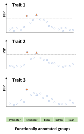
Figure 1: A multi-trait fine mapping example that motivates the development of our method. Y-axis refers to the posterior inclusion probability (PIP) and X-axis refers to the position of SNPs on the genome. The two causal variants are symbolized by diamond or triangle. The dashed line indicates a PIP threshold above which a variant can be regarded as causal to that trait. Variants are shaded orange when they pass the PIP threshold.

In this paper, we develop a novel Bayesian indicator variable selection method in multivariate regression model when there are a large number of grouped predictors targeting at multiple correlated responses. Our method is built upon existing Bayesian indicator variable selection methods first proposed by Kuo and Mallick, (1998) as an alternative reparameterization of spike-and-slab prior, and later developed by Sillanpää and Bhattacharjee, (2005, 2006); Xu and Ghosh, (2015); Zhu et al., (2019) for group-level selection with wide genetic and multi-omics applications. Liquet et al., (2017) proposed multivariate sparse group selection method with spike-and-slab prior to select predictors with group structure associated with several correlated outcome variables. Wang et al., (2020) proposed a Bayesian analogue of traditional stepwise selection methods with potential extension to select variables simultaneously for multiple outcomes. Other Bayesian methods more specifically designed for fine mapping were also developed to identify pleiotropic SNPs that are potentially causal variants of multiple traits (Stephens,, 2013; Hormozdiari et al.,, 2016; Kichaev et al.,, 2017; Schaid et al.,, 2018). Several important issues in variable selection with multiple responses, however, are not well addressed in these methods. First, all these methods assume common predictors of all the responses. In reality, heterogeneity usually exists so a predictor might be predictive of some responses but not the others. Secondly, as the dimension of response grows, it becomes an imperative task to identify subset(s) of responses that are most impacted by the predictor which might help generate new hypotheses. For example, it is appealing to identify the subset of neuroimaging phenotypes (possibly in spatial proximity and with similar functional roles) certain SNPs target at to improve our understanding of the heterogeneous genetic effect on the brain. Lastly, incorporation of background knowledge to guide variable selection has been repeatedly emphasized in genomic application and can be equally important when selecting predictors for multiple responses. This is especially critical in fine mapping. For example, the group structure as defined by physical location, functional annotation, haplotype or LD patterns is useful in narrowing down the selection into smaller sets of functionally relevant SNPs; the probability of a variant being causal is related to existing knowledge stored in reference database about the variant, e.g. whether the variant is an expression quantitative trait loci (eQTL) or other multi-omics QTL (Schaid et al.,, 2018). Incorporating multiple lines of evidence of prior knowledge will help improve causal variant selection performance and draw more reliable interpretation and conclusion.

To the best of our knowledge, our method is the first Bayesian indicator variable selection method that selects predictors for multiple correlated responses with possible heterogeneity. Comparing to existing methods, our method is featured by the following characteristics: (1) it conducts variable selection at both individual feature and group levels, and the selection is specific to each response, thus allowing the heterogeneity across multiple responses; (2) we introduce a new concept of subset PIP in genetic fine mapping to prioritize causal variants that target at subset(s) of traits and use it to make inference; (3) under the full Bayesian framework, our method is also flexible in incorporating prior biological knowledge into several parts of the model to guide grouping and weight the causal probability. In addition, we showed the posterior median estimator of the regression coefficients in our model is a soft thresholding estimator with selection consistency and asymptotic normality. We performed extensive simulations comparing our proposed method to existing multivariate regularization, Bayesian variable selection and fine-mapping methods. We applied our method to a multi-trait fine mapping problem and identified several important variants that target at multiple addictive behaviors and their risk factors. The paper is organized as follows. In Section 2, we review Bayesian variable selection methods, propose our model and its key features, investigate its theoretical properties, provide a Gibbs sampler and propose subset PIP for posterior inference. In Section 3, we list key benefits and downfalls of pre-existing methods. In Section 4, we show our model’s performance in extensive simulations. In Section 5 we show a real data example and in Section 6 we provide discussion on the potential extension of our method in future studies.

2 Methods

2.1 Review of Bayesian variable selection methods: spike and slab and indicator variable selection models

We first consider a linear regression model for a univariate response $Y_{i}$ with $p$ covariates $X_{ij},j=1,\ldots,p$:

$$Y_{i}=\sum_{j=1}^{p}\beta_{j}X_{ij}+\epsilon_{i},\quad\epsilon_{i}\sim N(0,\sigma^{2}),$$ (2.1)

for samples $i=1,2,\ldots,n$. The data are assumed to be centered so the intercept can be ignored. The spike and slab model (Mitchell and Beauchamp,, 1988; George and McCulloch,, 1993), among the most popular Bayesian variable selection methods, imposes the following prior on each regression coefficient $\beta_{j}$:

$$\begin{split}\beta_{j}&\sim(1-\gamma_{j})N(0,\tau_{j}^{2})+\gamma_{j}N(0,c_{j}^{2}\tau_{j}^{2});\\ \gamma_{j}&\sim Bern(\pi_{j}),\end{split}$$ (2.2)

where $\tau_{j}^{2}$ is usually chosen very small, and $c_{j}^{2}$ is usually chosen large. $\gamma_{j}$ indicates whether the $j$th covariate is predictive of the outcome: when $\gamma_{j}=1$, $\beta_{j}$ is drawn from the wide slab part $N(0,c_{j}^{2}\tau_{j}^{2})$; when $\gamma_{j}=0$, $\beta_{j}$ is drawn from the close-to-zero spike part. This prior will encourage a sparse model shrinking coefficients under spike towards zero.

Kuo and Mallick, (1998) proposed an indicator variable selection model as an alternative to spike and slab model. The idea is to attach an indicator variable to each coefficient for model selection:

$$\begin{split}Y_{i}&=\sum_{j=1}^{p}\beta_{j}\gamma_{j}X_{ij}+\epsilon_{i},\epsilon_{i}\sim N(0,\sigma^{2});\\ \beta_{j}&\sim N(0,s^{2}),\qquad\gamma_{j}\sim Bern(\pi_{j}).\\ \end{split}$$ (2.3)

When $\gamma_{j}=1$, the $j$th predictor is included in the regression model, when $\gamma_{j}=0$, the $j$th predictor is omitted from the model. Note that the indicator variable selection model can be shown to be equivalent to the spike and slab model when the spike and slab prior is imposed on $\beta_{j}\gamma_{j}$ and the spike distribution is replaced by a Dirac delta function $\delta_{0}(.)$ with all mass at 0.

In many cases, predictors naturally form groups. Genetic variants located in close physical proximity and genes in the same functional pathway are all examples of groups. It is usually of interest to identify which groups of predictors are selected and which predictors are selected within each group. Xu and Ghosh, (2015) and Zhang et al., (2014) extended the spike and slab model to encourage shrinkage of coefficients both at the group level and within groups. For group selection, the model is largely the same as the regular spike and slab model, except that coefficients are now considered in groups so that the prior is given at the group level:

$$\begin{split}\boldsymbol{\beta}_{g}&=\textbf{V}_{g}^{1/2}\textbf{b}_{g},\quad\textbf{V}_{g}^{1/2}=\mathrm{diag}(\tau_{g1},\ldots,\tau_{gm_{g}});\\ \textbf{b}_{g}&\sim(1-\pi_{1})\delta_{0}(.)+\pi_{1}N_{m_{g}}(\textbf{0},\textbf{I}_{m_{g}});\\ \tau_{gj}&\sim(1-\pi_{2})\delta_{0}(.)+\pi_{2}N^{+}(0,s^{2}),\end{split}$$ (2.4)

where $g$ is the group index and $m_{g}$ is the number of predictors in $g$th group. $\boldsymbol{\beta}_{g}=(\beta_{g1},\ldots,\beta_{gm_{g}})$ and $N^{+}$ denotes a normal distribution truncated below at 0. Such a model can be reparameterized as:

$$\begin{split}\beta_{gj}=\gamma_{g}^{(1)}\gamma_{gj}^{(2)}b_{gj},\quad\gamma_{g}^{(1)}&\sim Bern(\pi_{1}),\quad\gamma_{gj}^{(2)}\sim Bern(\pi_{2}),\\ b_{gj}&\sim N(0,s^{2}),\end{split}$$ (2.5)

which can be treated as an extension of the original indicator variable selection model to group selection as adopted by other authors (Chen et al.,, 2016; Zhu et al.,, 2019).

All the above models are restricted to univariate response. In applications, it is common to jointly analyze several correlated outcome measures together (e.g. multiple diagnostic tests for the same disease). Consider a multivariate regression model with $q$ correlated responses Y given covariate matrix X:

$$\textbf{Y}=\textbf{XB}+\boldsymbol{\epsilon},\quad\boldsymbol{\epsilon}\sim MN_{n\times q}(0,\textbf{I}_{n}\otimes\Sigma),$$ (2.6)

where $\Sigma$ is the covariance matrix for the $q$ responses. Following the formulation by Xu and Ghosh, (2015), Liquet2017 provides a full Bayesian multivariate spike and slab model which allows sparsity both at group level and within groups:

$$\begin{split}\textbf{B}_{g}&=\textbf{V}_{g}^{\frac{1}{2}}\tilde{\textbf{B}}_{g},\quad\textbf{V}^{\frac{1}{2}}_{g}=\mathrm{diag}\{\tau_{g1},...,\tau_{gm_{g}}\};\\ Vec(\tilde{\textbf{B}}_{g}^{T}|\Sigma,\tau_{g},\pi_{1})&\sim(1-\pi_{1})\delta_{0}(.)+\pi_{1}MN_{m_{g}\times q}(\textbf{0},\textbf{I}_{m_{g}}\otimes\Sigma);\\ \tau_{gj}&\sim(1-\pi_{2})\delta_{0}(.)+\pi_{2}N^{+}(0,s^{2}),\\ \end{split}$$ (2.7)

where $\textbf{B}_{g}$ is the $m_{g}\times q$ regression coefficient matrix for group $g$. In this model, both group selection and within group selection are common to all $q$ responses but not specific to any single response.

The spike and slab and indicator variable selection models and their variants have been a popular choice for variable selection and widely used for genetic fine mapping and related applications (Stephens,, 2013; Kichaev et al.,, 2014; Hormozdiari et al.,, 2016; Fang et al.,, 2018; Schaid et al.,, 2018). With univariate response, the spike and slab model and indicator selection model can be shown equivalent thus perform equally well for individual and group-level selection of predictors (Kuo and Mallick,, 1998; Xu and Ghosh,, 2015). With multivariate response, Liquet2017’s multivariate spike and slab model considers predictor selection common to all responses. However, this is a rather strong assumption which does not always hold in real application. For example, in fine mapping, heterogeneity might exist for different responses, e.g. certain causal variants might target at only a subset of traits but not others. Comparing to the original spike and slab formulation, the indicator selection model has more flexibility to be extended to response-specific predictor selection. This has motivated us to propose a novel multivariate indicator variable selection model with response specific feature selection that can be applied to multi-trait fine mapping problem and potentially other related problems. As we will see next, in multivariate case, the proposed indicator variable selection model is not equivalent to Liquet et al., (2017)’s multivariate spike and slab model.

2.2 A multivariate Bayesian indicator variable selection model

Under the same multivariate linear regression setting in Equation (2.6), we assume there are $p$ predictors that are potentially predictive of $q$ correlated responses. In fine mapping, this could correspond to $p$ SNPs in a local genomic region that might be causing the change in $q$ related phenotypes/traits. Denote by Y an $n\times q$ matrix of responses and X an $n\times p$ matrix of predictors, suppose the $p$ predictors are divided into $G$ disjoint groups (e.g. functionally annotated regions and LD blocks of SNPs in fine mapping) where $m_{g}$ is the number of predictors in $g$th group (i.e. $p=\sum\limits_{g=1}^{G}m_{g}$). We propose the following full Bayesian hierarchical model to encourage variable selection both at group level and within group, and specific to each response:

$$\begin{split}\textbf{Y}&\sim MN_{n\times q}(\textbf{XB},\textbf{I}_{n}\otimes\Sigma),\quad\textbf{B}=\textbf{Z}\odot\textbf{b},\quad\Sigma\sim\mathrm{IW}(q,\textbf{I});\\ z_{gj,k}&=\alpha_{g}\gamma_{gj}\omega_{gj,k},\quad g=1,\ldots,G;\quad j=1,\ldots,m_{g};\\ &\qquad\qquad\qquad\qquad k=1,\ldots,q;\\ \vec{b}_{gj}&\sim N_{q}(\vec{0},s^{2}\Sigma),\quad g=1,\ldots,G;\quad j=1,\ldots,m_{g};\\ \alpha_{g}&\sim\mathrm{Bern}(\pi^{(\alpha)}),\quad\gamma_{gj}\sim\mathrm{Bern}(\pi_{g}^{(\gamma)}),\quad\omega_{gj,k}\sim\mathrm{Bern}(\pi_{gj}^{(\omega)}),\end{split}$$ (2.8)

where $\textbf{B}=\{(\beta_{gj,k}),g=1,\ldots,G;j=1,\ldots,m_{g};k=1,\ldots,q\}$, $\textbf{Z}=\{(z_{gj,k}),g=1,\ldots,G;j=1,\ldots,m_{g};k=1,\ldots,q\}$, $\textbf{b}=\{(b_{gj,k}),g=1,\ldots,G;j=1,\ldots,m_{g};k=1,\ldots,q\}$, $\vec{b}_{gj}=(b_{gj,1},\ldots,b_{gj,q})^{T}$, $\mathrm{IW}(q,\textbf{I})$ refers to the inverse Wishart distribution with scale matrix I and degree of freedom $q$. Each component in B is a product of selection indicator in Z matrix and the underlying effect size in b matrix, where $\odot$ represents the Hadamard (element-wise) multiplication. Each selection indicator $z_{gj,k}$ is a product of three indicator variables: $\alpha_{g}$ which indicates whether $g$th group of predictors is selected, $\gamma_{gj}$ which indicates whether $j$th feature in $g$th group is selected and $\omega_{gj,k}$ which indicates whether $j$th feature in $g$th group is selected specifically for $k$th response. Figure 2 shows the structure of the matrix of response Y, the matrix of predictors X and the coefficient matrix B and the correspondence of the three selection indicators to the components in B. Note that $z_{gj,k}=1$ only when $\alpha_{g}=\gamma_{gj}=\omega_{gj,k}=1$, i.e. the group that includes the predictor is selected, the predictor is selected within the group, and the selection is specific to that response.

We assume noninformative conjugate priors on the hyperparameters: $\pi^{(\alpha)}\sim\mathrm{Beta}(1,1)$, $\pi^{(\gamma)}_{g}\sim\mathrm{Beta}(1,1)$, $\pi^{(\omega)}_{gj}\sim\mathrm{Beta}(1,1)$ and $p(s^{2})\propto IG(0.01,0.01)$, where $IG(.)$ refers to inverse gamma distribution. In many applications, whether we select a group of predictors or an individual predictor will largely depend on prior biological knowledge. For example, in fine mapping, a variant is more likely to be causal if it plays some regulatory role, i.e. being an eQTL or multi-omics QTL. In this case, we need to impose more informative priors on the hyperparameters $\pi^{(\alpha)}$, $\pi^{(\gamma)}_{g}$ and $\pi^{(\omega)}_{gj}$. We show one example of putting informative prior on $\pi^{(\gamma)}_{g}$ to incorporate regulatory QTL information from reference database to prioritize causal variant selection in fine mapping in this paper (see Section 2.3 for details) but the general idea also applies to the other hyperparameters.

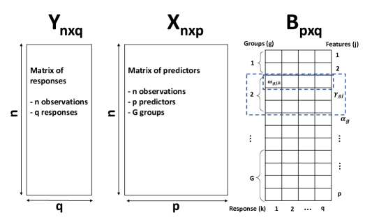
Figure 2: Structure of the matrix of response Y, the matrix of predictor X, the coefficient matrix B in the proposed model. $\alpha_{g}$, $\gamma_{gj}$ and $\omega_{gj,k}$ correspond to the indicators for selecting the group, individual feature within the group and selecting the feature for a specific response, respectively.

REMARKS:
1. The three indicators play different roles in feature selection of the hierarchical model as indicated in Fig 2: $\alpha_{g}$ controls the selection at the group level, $\gamma_{gj}$ controls the selection of individual predictor within the group, and $\omega_{gj,k}$ selects the predictor specific to each response. The product $\alpha_{g}\gamma_{gj}$ has the same formulation as in Xu and Ghosh, (2015)’s bi-level sparse group selection with spike and slab prior, however, such a product does not discriminate the heterogeneous predictor effect on different responses. Adding $\omega_{gj,k}$ to the product will help identify which response(s) each predictor targets at. Under this setting, both the important features and the responses they target at can be identified. Note that this is very different from performing feature selection in a separate regression for each response, where no information can be shared across the different regressions.

2. In this model, instead of putting a multivariate spike and slab prior directly on the coefficient matrix of B as in Liquet et al., (2017), we impose element-wise prior on each coefficient by extending Kuo and Mallick, (1998)’s indicator variable selection model to multivariate case. This, however, does not imply the independence between predictors or responses in the selection. The predictors belonging to the same group are more likely to be selected together since they are under the control of a common group indicator $\alpha_{g}$, while the same predictors are more likely to be selected for different responses due to the common individual predictor indicator $\gamma_{gj}$.

3. For the covariance matrix $\Sigma$, we assume it to follow a noninformative conjugate prior, the inverse Wishart distribution with degree of freedom equal to $q$ and scale matrix be the identity matrix $I$. $q$ has to be greater than 2 to ensure the existence of $\textbf{E}(\Sigma)$. Such prior works well when we have a relatively large sample size (i.e. $n$ is large) and moderate number of responses (i.e. $q$ not too large), which holds true in genetic fine mapping. In other applications such as in transcriptomic studies, sample size is usually small, we might need to consider simultaneous variable selection and covariance selection by posing extra spike and slab or indicator variable priors on $\Sigma$ as in Deshpande et al., (2019). The performance will need to be further investigated in future studies.

4. We assume the effect size vector $\vec{b}_{gj}$ has a prior multivariate normal distribution with covariance matrix $\Sigma$ scaled by a common factor $s^{2}$. Alternatively, we can assume a group specific $s_{g}^{2}$ or feature specific variance $s_{gj}^{2}$ to allow for more heterogeneous effect sizes. This is like the fixed effect model vs. random effect model comparison in the meta-analysis literature (Borenstein et al.,, 2010). We investigated and compared the performance in simulations and did not find clear difference between the two priors. For computational efficiency, we will stick to the prior with the common scaling factor in this paper.

5. When $z_{gj,k}=0$, at least one of the three binary indicators $\alpha_{g}$, $\gamma_{gj}$ and $\omega_{gj,k}$ is equal to zero. However, the different situations (e.g. whether $\alpha_{g}=\gamma_{gj}=\omega_{gj,k}=0$ or only $\alpha_{g}=0$) are not identifiable by likelihood. This could be less of an issue since the selection is eventually determined by the product $z_{gj,k}$ specific to each response for each variable. Thus, we followed from Zhu et al., (2019) and decided not to put any constraints in the prior to identify individual indicators at a price that these indicators might sometimes not be directly interpretable.

6. The current model focuses on a set of normally distributed continuous outcomes. Extension to binary, categorical and other types of outcomes or mixed types of outcomes is possible, though the multivariate distribution of correlated non-normal outcomes is not as well defined as normal outcomes. Alternatively, one can adopt data augmentation algorithm (Albert and Chib, (1993)) by introducing latent variable for each outcome and build the hierarchy on the latent variables. For example, for binary outcome, we can introduce a latent continuous variable $T_{i,k}(i=1,\ldots,n,k=1,\ldots,q)$ to replace the binary $Y_{i,k}$ in the regression, i.e. we assume $Y_{i,k}=1$ if $T_{i,k}\geq 0$ and $Y_{i,k}=0$ otherwise, and $\textbf{T}\sim MN_{n\times q}(\textbf{XB},\textbf{I}_{n}\otimes\Sigma)$.

7. Similar to Xu and Ghosh, (2015) and Liquet et al., (2017), our method also assumes predictors naturally form groups, and such a bi-level selection has demonstrated a significant improvement in variable selection and prediction. However, the definition of groups could be subjective and context-dependent. In addition, there will be quite a few predictors which do not belong to any groups known as “singletons”. For singletons, $\alpha_{g}$ and $\gamma_{gj}$ will always be equal to each other.

8. In practice, important covariates that might confound the selection results need to be included and carefully addressed. Since our method is built upon a very general multivariate regression model, any covariates can be readily adjusted in the model for their additive or non-addictive effects.

2.3 Prioritizing selection using existing biological knowledge

In this subsection, we show an example of incorporating biological knowledge in the prior distribution of hyperparameters $\pi$’s in fine mapping application. Detailed prior setting needs to be evaluated case-by-case for each application and we do not further discuss all the possibilities here.

eQTLs are genomic loci that explain variation in gene expression levels. Genetic studies have found SNPs associated with complex traits more likely to be eQTLs than other SNPs on genotype arrays with the same allele frequencies (Nicolae et al.,, 2010). Thus, it is natural to put more weights on the eQTLs identified from large-scale genomic studies when determining causal variants in fine mapping. In our study, we incorporate eQTL information from reference database (e.g. ENCODE, ROSMAP, GTEx, QTLbase) and consider the following prior on the selection indicator $\gamma_{gj}$ to prioritize the eQTLs:

$$\begin{split}\gamma_{gj}\sim\text{Bern}(\pi^{(\gamma)}_{gj}),\quad\Phi^{-1}(\pi^{(\gamma)}_{gj})=d_{0}+d_{1}A_{gj},\quad d_{0}&\sim N(0,\sigma^{2}),\\ d_{1}&\sim N(\mu_{d},\tau^{2}),\end{split}$$ (2.9)

where $A_{gj}$ is a binary variable indicating whether $j$th feature in $g$th group is an eQTL based on the reference database. $\Phi^{-1}(.)$ is the inverse of CDF of standard normal distribution, a.k.a. probit link in Bayesian literature to achieve conjugacy (Albert and Chib,, 1993). We note that there is some flexibility in setting prior for $d_{1}$, and in particular we may control the relative strength/emphasis of eQTL information by varying the value of the prior mean $\mu_{d}$. If there is a strong belief that eQTL should indicate causality, the prior mean $\mu_{d}$ may be set more positive value so the probability of the corresponding eQTL being a causal variant is increased. Alternatively, one can use gamma distribution truncated below zero as the prior for $d_{1}$ to put moderately larger weights on eQTLs. In the real data application, we set $\mu_{d}=0$. Lastly we allow noninformative priors on $\sigma^{2}$ and $\tau^{2}$, e.g. following Jeffreys priors. Similar formulation for incorporating functional annotation or eQTL information in fine mapping has also been seen in Kichaev et al., (2017).

All the parameters in the model have closed form posterior distributions, thus we use a Gibbs sampler to sample from their posterior distributions. The detailed conditional posterior distributions of all the parameters can be found in section 1 of the Supplement.

2.4 Posterior median as a soft thresholding estimator

It has been shown that under mild conditions, the posterior median estimator of normal mean sample with spike-and-slab prior is a soft-thresholding estimator with desired oracle (i.e. selection consistency) and asymptotic normality properties (Johnstone and Silverman,, 2004; Xu and Ghosh,, 2015). Liquet et al., (2017) generalized the thresholding results to multivariate response variable and Zhu et al., (2019) showed the results for the equivalent reparametrized indicator variable selection model. In this paper, we will also use posterior median estimator for both variable selection and parameter estimation. In this subsection, we will show that the posterior median estimator is a soft thresholding estimator in our model and we will prove its oracle and asymptotic normality properties.

Assume that the design matrix X is orthogonal (that is, $\textbf{X}^{T}\textbf{X}=n\textbf{I}_{p}$), consider the model described in equation (2.8) with fixed $\Sigma$ and $s^{2}$, it can be shown that the marginal posterior distribution of $\beta_{gj,k}$ given the observed data is a spike and slab distribution (see derivation in section 2 of the Supplement):

$$\beta_{gj,k}|\textbf{X},\textbf{Y}\sim l_{gj,k}N((1-D_{n})\hat{\beta}_{gj,k}^{LS},\frac{1-D_{n}}{n}\Sigma_{kk})+(1-l_{gj,k})\delta_{0}(\beta_{gj,k}),$$ (2.10)

where $\hat{\beta}_{gj,k}^{LS}$ is the least squares estimator of $\beta_{gj,k}$, $D_{n}=\frac{1}{1+ns^{2}}$, $\Sigma_{kk}$ is the $k$th diagonal element of $\Sigma$ and

$$\begin{split}l_{gj,k}&=P(z_{gj,k}=1|rest)\\ &=\frac{\pi_{gj}^{*}(1+ns^{2})^{\frac{1}{2}}\exp{\left[(1-D_{n})n\Sigma_{kk}^{-1}(\hat{\beta}_{gj,k}^{LS})^{2}\right]}}{\pi_{gj}^{*}(1+ns^{2})^{\frac{1}{2}}\exp{\left[(1-D_{n})n\Sigma_{kk}^{-1}(\hat{\beta}_{gj,k}^{LS})^{2}\right]}+(1-\pi_{gj}^{*})},\end{split}$$ (2.11)

where $\pi_{gj}^{*}=\pi^{(\alpha)}\pi_{g}^{(\gamma)}\pi_{gj}^{(\omega)}$.

The resulting posterior median is a soft thresholding estimator $\hat{\beta}_{gj,k}^{Med}=\mathrm{Med}(\beta_{gj,k}|\textbf{X},\textbf{Y})$ given by (see the derivation in section 3 of the Supplement):

$$\begin{split}\hat{\beta}_{gj,k}^{Med}=\mathrm{sgn}(\hat{\beta}_{gj,k}^{LS})&\Biggl{(}(1-D_{n})|\hat{\beta}_{gj,k}^{LS}|-\\ &\frac{\sqrt{\Sigma_{kk}}}{\sqrt{n}}\sqrt{1-D_{n}}\Phi^{-1}\left(\frac{1}{2\mathrm{max}\left(l_{gj,k},\frac{1}{2}\right)}\right)\Biggr{)}_{+},\end{split}$$ (2.12)

where $\mathrm{sgn}(\cdot)$ is the sign function, $\Phi$ is the CDF of the standard normal distribution and $(x)_{+}$ takes the value of $x$ if $x>0$ and zero otherwise. This is similar to the lasso estimator (Tibshirani,, 1996) which can be expressed as a soft-thresholding estimator under orthogonal design. The results also match well with that by Xu and Ghosh, (2015) for univariate response and Liquet et al., (2017) for multivariate response vector, except that what we derive is specific to each response in the multivariate case.

Next, we show the asymptotic properties of the posterior median estimator $\hat{\beta}_{gj,k}^{Med}$. Let $\mathbf{B}^{0}$ and $\beta_{gj,k}^{0}$ be the true values of $\mathbf{B}$ and $\beta_{gj,k}$. Define $\mathcal{A}=(I(\beta_{gj,k}^{0}\neq 0),g=1,\ldots,G;j=1,\ldots,m_{g};k=1,\ldots,q)$ as the indicator vector of non-zero covariates in the true model and let $\mathcal{A}_{n}=(I(\hat{\beta}_{gj,k}^{Med}\neq 0),g=1,\ldots,G;j=1,\ldots,m_{g};k=1,\ldots,q)$ be the indicator vector of non-zero covariates from the posterior median estimator.

Under the orthogonal design, the posterior median estimator has the oracle property, i.e. variable selection consistency.

Theorem 2.1 (Asymptotic Properties of the Posterior Median Estimator).

Assuming an orthogonal design matrix $\textbf{X}^{T}\textbf{X}=n\textbf{I},\hskip 2.5pt\sqrt{n}s^{2}\rightarrow\infty$ and $\frac{\log(s^{2})}{n}\rightarrow 0$ as $n\rightarrow\infty$, then the posterior median estimator in our model has the following asymptotic properties:

$\lim_{n\rightarrow\infty}P(\mathcal{A}_{n}=\mathcal{A})=1$ (Selection consistency)

$\sqrt{n}(\widehat{\mathbf{B}}_{\mathcal{A}}^{Med}-\mathbf{B}_{\mathcal{A}}^{0})\rightarrow MN(\mathbf{0},\mathbf{I}\otimes\Sigma)$ (Asymptotic normality)

Detailed proof of this theorem can be found in section 4 of the Supplement.

2.5 Posterior inference: Bayesian false discovery rate (BFDR) and subset posterior inclusion probabilities (subset PIP)

Practical implementations of Bayesian variable selection approaches typically summarize the posterior distribution by the marginal posterior inclusion probability (PIP) of each variable and draws inference (Kruschke,, 2014). Adopting the conjunction hypothesis setting $H_{0}:\underset{k}{\cap}\{\beta_{gj,k}=0\}$ vs. $H_{a}:\underset{k}{\cup}\{\beta_{gj,k}\neq 0\}$ (a.k.a. omnibus hypothesis), we can define PIP for $j$th predictor in group $g$ in our model as:

$$PIP_{gj}\coloneqq P_{gj}(H_{a}|\textbf{X},\textbf{Y})=P(\underset{k}{\cup}\{\beta_{gj,k}\neq 0\}|\textbf{X},\textbf{Y}).$$ (2.13)

To adjust for multiplicity, we followed from Newton et al., (2004) and proposed to control the false discovery rate (FDR) at individual predictor level in Bayesian model by defining Bayesian false discovery rate (BFDR) as:

$$BFDR(t)=\frac{\sum_{g=1}^{G}\sum_{j=1}^{m_{g}}P_{gj}(H_{0}|\textbf{X},\textbf{Y})d_{gj}(t)}{\sum_{g=1}^{G}\sum_{j=1}^{m_{g}}d_{gj}(t)},$$ (2.14)

where $P_{gj}(H_{0}|\textbf{X},\textbf{Y})=P(\underset{k}{\cap}\{\beta_{gj,k}=0\}|\textbf{X},\textbf{Y})=1-PIP_{gj}$ is the probability of a variable not being selected for any responses given the data and $d_{gj}(t)=I\{P_{gj}(H_{0}|\textbf{X},\textbf{Y})<t\}$. BFDR can be controlled at a certain $\alpha$ level by tuning $t$.

We can follow the conjunction hypothesis setting to select the top predictors with BFDR controlled. However, the rejection of the conjunction of null hypotheses is often too general to be scientifically meaningful, i.e. we only know the predictor is associated with at least one response but do not know which ones. In reality, heterogeneity usually exists among the different responses. For example, in genetic fine mapping of regional neuroimaging phenotypes, we are interested in knowing what subset of regional traits that each causal variant targets at, to generate new hypotheses. To facilitate scientific finding and interpretability, we propose a novel concept of subset PIP to help select the best possible subset of responses each predictor targets at.

Denote by $\mathcal{M_{S}}\subset\{1,2,\ldots,q\}$ a subset of response indices a predictor targets at, we define the following subset PIP for each predictor, $1\leq j\leq m_{g},1\leq g\leq G$:

$$PIP_{gj}^{\mathcal{M_{S}}}=P(\beta_{gj,k}\neq 0,\hskip 2.5pt\text{for}\hskip 2.5ptk\in\mathcal{M_{S}}|\textbf{X},\textbf{Y}).$$ (2.15)

For each predictor, we can calculate $PIP_{gj}^{\mathcal{M_{S}}}$ for all possible $2^{q}-1$ subsets and identify the best subset as the one that maximizes $PIP_{gj}^{\mathcal{M_{S}}}$ (i.e. $\mathcal{M_{S}}_{gj}^{*}=\mathrm{argmax}_{\mathcal{M_{S}}}PIP_{gj}^{\mathcal{M_{S}}}$). However, size bias exists wherein smaller subset tends to have higher subset PIP. For example, a predictor might target at three responses with stronger effects on two responses but relatively weaker effects on the third one. Using the subset PIP directly calculated from equation (2.15) will favor the selection of the first two responses though the underlying truth is to select all the three responses. To resolve this issue, we propose a permutation based method to generate an empirical reference distribution of $PIP_{gj}^{\mathcal{M_{S}}}$ with the same subset size for fair comparison and best subset selection.

We randomly shuffle all elements in the estimated $\widehat{\textbf{B}}$ matrix for a total of $R$ times, so we generate $R$ matrices of $\widehat{\textbf{B}}^{r},r=1,\ldots,R$. For each permuted matrix $\widehat{\textbf{B}}^{r}$, we recalculate $PIP_{gj}^{\mathcal{M_{S}},r}$ for each subset $\mathcal{M_{S}}$. We then summarize all the permutations into a subset specific Z-score: $Z_{gj}^{\mathcal{M_{S}}}=\frac{PIP_{gj}^{\mathcal{M_{S}}}-\frac{1}{R}\sum_{r=1}^{R}PIP_{gj}^{\mathcal{M_{S}},r}}{\sqrt{\frac{1}{R}\sum_{r=1}^{R}(PIP_{gj}^{\mathcal{M_{S}},r}-\left(\frac{1}{R}\sum_{r=1}^{R}PIP_{gj}^{\mathcal{M_{S}},r}\right)})^{2}}.$

The best subset of responses each predictor targets at can be identified by maximizing the corresponding Z-score, i.e. $\mathcal{M_{S}}_{gj}^{*}=\mathrm{argmax}_{\mathcal{M_{S}}}Z_{gj}^{\mathcal{M_{S}}}$. Since the Z-scores are calculated by comparing to the reference distribution of the same subset size, the size bias is mitigated. The method is summarized below in Algorithm 1.

Algorithm 1 Permutation method for best subset selection

1:Input: posterior median estimate of coefficient matrix $\widehat{\textbf{B}}$

2:Output: The best response subset $\mathcal{M_{S}}_{gj}^{*}$ for each feature, $1\leq j\leq m_{g},1\leq g\leq G$

3:

4:for $g\leftarrow 1$ to $G$ do

5:     for $j\leftarrow 1$ to $m_{g}$ do

6:         for $\mathcal{M_{S}}\subset\{1,2,\ldots,q\}$ do

7:              Calculate $PIP_{gj}^{\mathcal{M_{S}}}=P(\hat{\beta}_{gj,k}\neq 0,\hskip 2.5pt\text{for}\hskip 2.5ptk\in\mathcal{M_{S}}|\textbf{X},\textbf{Y})$, where $\hat{\beta}_{gj,k}$ is the (gj,k)th element in $\widehat{\textbf{B}}$

8:         end for

9:     end for

10:end for

11:for $r\leftarrow 1$ to $R$ do

12:     Obtain a permuted matrix $\widehat{\textbf{B}}^{r}$ by randomly shuffling all elements in $\widehat{\textbf{B}}$

13:end for

14:for $g\leftarrow 1$ to $G$ do

15:     for $j\leftarrow 1$ to $m_{g}$ do

16:         for $\mathcal{M_{S}}\subset\{1,2,\ldots,q\}$ do

17:              Calculate

$$Z_{gj}^{\mathcal{M_{S}}}=\frac{PIP_{gj}^{\mathcal{M_{S}}}-\frac{1}{R}\sum_{r=1}^{R}PIP_{gj}^{\mathcal{M_{S}},r}}{\sqrt{\frac{1}{R}\sum_{r=1}^{R}(PIP_{gj}^{\mathcal{M_{S}},r}-\left(\frac{1}{R}\sum_{r=1}^{R}PIP_{gj}^{\mathcal{M_{S}},r}\right)})^{2}},$$

where $PIP_{gj}^{\mathcal{M_{S}},r}$ is obtained the same way but from $\widehat{\textbf{B}}^{r}$

18:         end for

19:         Obtain $\mathcal{M_{S}}_{gj}^{*}=\mathrm{argmax}_{\mathcal{M_{S}}}Z_{gj}^{\mathcal{M_{S}}}$ for each predictor

20:     end for

21:end for

22:return $\mathcal{M_{S}}_{gj}^{*}$

REMARK:
In this paper, we show PIP defined at individual predictor level. With the inclusion of indicators at three different levels in our model, it is flexible to also define the PIP at the group level to select groups of associated predictors. Since it is not the focus of our method, we will not further discuss it here and details will be left to future studies.

3 Other related methods

Many multivariate Bayesian and regularization methods have been developed to perform individual-level or group-level variable selection with multiple related responses for general application. Here, we summarize the main features and limitations of several related methods as compared to our method (namely Multivariate Bayesian Indicator Variable Selection (MBIVS)) below and in Table 1. In addition, we also include popular fine-mapping methods (mainly Bayesian model based) that can handle multiple traits for comparison.

• Multivariate Bayesian variable selection methods:

  • Multvariate Bayesian Group Lasso with Spike-and-Slab Prior (MBGL-SS) (Liquet et al.,, 2017): This multivariate model is based on a Bayesian group lasso model with an independent spike-and-slab prior for each group variable for group-level features selection, however, this model does not select features within the groups, and all grouped features selected are common to all responses.

  • Multivariate Bayesian Sparse Group Spike-and-Slab (MBSGS) (Liquet et al.,, 2017): This is a second model proposed in Liquet et al., (2017) and a multivariate implementation of the spike-and-slab model as given in Equations 2.6 and 2.7, which allows sparsity both at group levels and within groups. However, the selected features or groups are still common to all responses thus the heterogeneity among the responses cannot be accounted for.

  • Multivariate Sum of Single Effects Regression (mvSuSIE) (Wang et al.,, 2020): This is a multivariate extension of the SuSIE model, which is a new formulation of Bayesian variable selection regression as an alternative to spike and slab prior. This method is also inspired by fine-mapping, but applicable to a wider range of applications. The mvSuSIE model selects variables simultaneously for multiple outcomes, but not specific to any subset of most related outcomes.

• Multivariate regularization methods:

  • REgularized Multivariate regression for identifying MAster Predictors (remMap) (Peng et al.,, 2010): This method adopted a mixed L1/L2 penalty to encourage the selection of “master” predictors that affect many response variables in multivariate linear regression. This method cannot incorporate any prior knowledge e.g. for fine mapping application, in addition, it cannot select features or groups specific to each response.

  • Multivariate sparse group lasso (MSGLasso): This method imposes a sparse group lasso like (L1+L2) penalty in a multivariate regression model setting with arbitrary grouping structure (Li et al.,, 2015). Same as remMap, this method cannot incorporate any prior information, nor perform response specific variable selection.

• Fine-mapping methods:

  • Causal Variants Identification in Associated Regions (CAVIAR) (Farhad et al.,, 2014): This Bayesian fine-mapping method directly models the LD structure in a genomic region to identify causal variants of interest. CAVAIAR has a constraint on the maximum number of causal variants that can be detected. It is designed for a single trait, but has been applied to multiple trait setting using average PIP.

  • Probalistic Annotation Integrator (PAINTOR) (Kichaev et al.,, 2017): This is a multivariate extension of the original Bayesian fine-mapping model for single trait (Kichaev et al.,, 2014) to target at multiple traits. PAINTOR directly models LD structure and is able to incorporate additional functional annotation data. Same as CAVIAR, PAINTOR also has a constraint of the maximum number of causal variants one can select.

  • mvBIMBAM (Stephens,, 2013): mvBIMBAM is a general framework to establish both direct and indirect associations between SNPs and a set of correlated outcomes. The main purpose of the model is to reveal the causal relationship between genetics and multiple phenotypes, so it does not perform well when there are many phenotypes (the possible number of causal relationships goes exponentially large as the number of outcomes increases). One other downside of this model is instead of using PIP that has better probabilistic interpretation, it uses Bayes factor for inference.

Method	Indiv. feature	Grouped	Response specific	Best response	Prior biol.	Constraint	Reference
	selection	feature selection	feature selection	subset selection	knowledge	free
MBGL-SS	N	Y	N	N	N	Y	Liquet et al., (2017)
MBSGS	Y	Y	N	N	N	Y	Liquet et al., (2017)
mvSuSIE	Y	Y	N	N	Y	Y	Wang et al., (2020)
remMap	Y	Y	N	N	N	Y	Peng et al., (2010)
MSGLasso	Y	Y	N	N	N	Y	Li et al., (2015)
CAVIAR	Y	N	N	N	Y	N	Farhad et al., (2014)
PAINTOR	Y	N	N	N	Y	N	Kichaev et al., (2017)
mvBIMBAM	Y	N	N	N	Y	Y	Stephens, (2013)
MBIVS	Y	Y	Y	Y	Y	Y	Our method

Table 1: A comparison of different multivariate variable selection methods. Indiv. feature selection: whether conducting individual level feature selection; Grouped feature selection: whether conducting group-level feature selection; Response specific feature selection: whether selecting features specific to each response; Best response subset selection: whether selecting the best subset of responses each feature targets at; Prior biol. knowledge: whether prior biological knowledge can be incorporated into the model; Constraint free: whether there is any constraint in software implementation.

4 Simulation

4.1 Simulation setting

In this section, we conduct simulation studies to evaluate the variable selection and prediction performance of our method. Since the primary motivation for our method is genetic fine mapping, we will simulate both genotype (X) and multivariate phenotype data (Y) to reflect the fine mapping application, though the method is readily applicable to data with multiple predictors and multiple responses in more general forms.

We start by simulating the genotype data X. To mimic the real genotype pattern, we follow from Wang et al., (2007); Han and Wei, (2013) and simulate the number of minor alleles for all SNPs with fixed minor allele frequency of 0.24 using latent Gaussian model with covariance matrix defined by the LD structure. To mimic the grouping and correlation structure in genotype data, we simulate LD blocks of SNPs where SNPs within the same block has fixed correlation $\rho_{\text{within}}=0.6$ and SNPs not in the same block has correlation $\rho_{\text{between}}=0.3$. We allow group sizes to vary, belonging to the set $\{5,10,20\}$.

To simulate the coefficient matrix B, we design five simulation scenarios for a comprehensive assessment of our method, by varying the level of sparsity (i.e. how many true causal variants that exist), the level of heterogeneity (i.e. homogeneous vs more heterogeneous responses), as well as the dimensionality (i.e. total number of variants as compared to sample size). Figure 3 shows a pattern of the coefficient matrix B in Scenarios (I)-(V).

Scenario I: Low dimension more sparse homogeneous. We consider $n=500$ samples and $p=100$ SNPs, and among them $s=5$ SNPs are true causal variants. For the true causal variants, we assume $\beta_{gj,k}=1$ for all traits ($1\leq k\leq q$). For the other SNPs, we assume $\beta_{gj,k}=0$ for all traits.

Scenario II: Low dimension less sparse homogeneous. We consider the same $n$ and $p$ as in scenario I but now consider less sparse case where $s=10$ SNPs are assumed to be true causal variants. For the true causal variants, we assume $\beta_{gj,k}=1$ for all traits ($1\leq k\leq q$). For the other SNPs, we assume $\beta_{gj,k}=0$ for all traits.

Scenario III: Low dimension more sparse heterogeneous. We consider the same $n$ and $p$ and $s$ as in scenario I, but instead of assuming the effects of causal variants to be the same across all traits, we now consider more heterogeneous case where different causal SNPs target at different subset of traits (see Fig 3). When a SNP is causal for a trait, it has a signal strength $\beta_{gj,k}=0.25$. Otherwise, $\beta_{gj,k}=0$.

Scenario IV: Low dimension less sparse heterogeneous. Similar to scenario III, but instead now we consider less sparse case where $s=10$ true causal variants and they target at varying number of traits in the model. Similar to scenario III, the signal strength when a SNP is causal for a trait is set to $\beta_{gj,k}=0.25$. Otherwise, $\beta_{gj,k}=0$.

Scenario V: High dimension less sparse heterogeneous. We consider the same $s=5$ true causal variants, with 2 causal variants having signal strength $\beta_{gj,k}=0.50$ and 3 causal variants having signal strength $\beta_{gj,k}=0.25$. Coefficient pattern across responses remains the same as in Scenario III, but now we assume a high-dimensional case with $n=300$ and $p=500$.

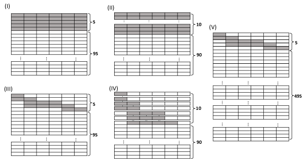
Figure 3: Layout plot of the coefficient matrix B pattern in Scenario (I)-(V). Black boxes indicate signal, white boxes indicate no signal.

For all scenarios, we assume $q=6$ correlated traits and the outcome $\textbf{Y}_{i}$ of each sample is simulated from $MN(\textbf{X}_{i}\textbf{B},\Sigma),i=1,\ldots,n$, where $\Sigma$ is the covariance matrix assuming to have a compound symmetry structure with fixed correlation $\rho=0.66$.

Each simulation is replicated for 100 times. To benchmark our method, we compare to the other multivariate Bayesian variable selection methods including Multivariate Bayesian Sparse Group Spike-and-Slab (MBSGS) (Liquet et al.,, 2017) and Multivariate Sum of Single Effects Regression (mvSuSIE) (Wang et al.,, 2020), the multivariate regularization methods including remMAP (Peng et al.,, 2010) and MSGLasso (Li et al.,, 2015), as well as the popular Bayesian fine mapping method CAVIAR (Farhad et al.,, 2014) and PAINTOR (Kichaev et al.,, 2017). Although mvBIMBAM is a multivariate method that may be used in genetic fine mapping applications, we choose not to include it in our comparisons because of its underlying goal to detect causal relationship among different responses which differs from the main goal of fine mapping. We assess the variable selection performance of each method using Area Under the ROC Curve (AUC) and the prediction performance using Mean Square Error (MSE). In addition, we also assess how the actual false discovery rate (FDR; the number of false positives/the number of claimed positives) and false omission rates (FOR; the number of false negatives/number of claimed negatives) are controlled at a nominal FDR level of 10%.

R was used to run all methods. For both our method and MBSGS, we ran for 7500 MCMC iterations with the first 2500 iterations as burn-in. To calculate sensitivity and specificity for remMap and MSGLasso, a variety of tuning parameters were considered. For a more comprehensive evaluation, we also performed the same simulations scenario with signal strength $\beta_{gj,k}=0.5$ and the results were included in the Supplement.

4.2 Simulation results

Table 2 shows the variable selection and prediction performance for all methods in all the five scenarios. When there are very few homogeneous signals (Scenario I), a majority of methods perform equally well with many having perfect AUC=1. Our MBIVS method and MBSGS perform better than fine mapping and regularization methods in FDR and FOR control as well as prediction. As the number of signals increases (Scenario II), the performance of fine mapping methods begins to drop. When the signals targeting at the responses become more heterogeneous (Scenario III-V), our MBIVS method outperforms the other Bayesian variable selection methods in variable selection, more specifically with higher AUC and lower FOR. This is partly because the other Bayesian methods (e.g. MBSGS and mvSuSIE) look at the multivariate response as a whole thus are less sensitive to heterogeneous signals especially when the signal strength is weak, while our method uses subset PIP for inference and is able to capture heterogeneous and weak signals. Note that increasing the dimension of the parameter space (Scenario V) will impact the performance of all methods as expected, but our method remains the best performer. When the signal strength increases, the performance of the other Bayesian variable selection methods improves and almost performs equally well as ours (see Table S1).

Scenario	Model	AUC	FDR	FOR	MSE
I	MBIVS	1.0 (0.00)	0.01 (0.00)	0.00 (0.00)	1.98 (0.01)
	MBSGS	1.0 (0.00)	0.02 (0.02)	0.00 (0.00)	1.97 (0.03)
	mvSuSIE	1.0 (0.00)	0.01 (0.00)	0.02 (0.00)	25.92 (0.02)
	CAVIAR	1.0 (0.00)	0.66 (0.00)	0.00 (0.00)	-
	PAINTOR	0.95 (0.00)	0.85 (0.00)	0.00 (0.00)	-
	remMAP	0.73 (0.00)	-	-	2.52 (0.03)
	MSGLasso	0.60 (0.00)	-	-	19.36 (0.03)
II	MBIVS	1.0 (0.00)	0.01 (0.00)	0.00 (0.00)	2.00 (0.02)
	MBSGS	1.0 (0.00)	0.08 (0.02)	0.00 (0.00)	2.00 (0.03)
	mvSuSIE	0.99 (0.00)	0.02 (0.01)	0.05 (0.00)	105.56 (0.04)
	CAVIAR	0.99 (0.00)	0.60 (0.00)	0.00 (0.00)	-
	PAINTOR	0.94 (0.00)	0.72 (0.00)	0.00 (0.00)	-
	remMAP	0.69 (0.00)	-	-	2.52 (0.03)
	MSGLasso	0.60 (0.00)	-	-	69.26 (0.06)
III	MBIVS	0.97 (0.00)	0.12 (0.02)	0.01 (0.01)	2.04 (0.01)
	MBSGS	0.90 (0.03)	0.11 (0.06)	0.02 (0.00)	1.99 (0.03)
	mvSuSIE	0.85 (0.01)	0.06 (0.02)	0.03 (0.00)	2.02 (0.01)
	CAVIAR	0.91 (0.01)	0.25 (0.03)	0.04 (0.00)	-
	PAINTOR	0.64 (0.01)	0.91 (0.00)	0.02 (0.00)	-
	remMAP	0.77 (0.01)	-	-	1.94 (0.03)
	MSGLasso	0.56 (0.00)	-	-	2.26 (0.01)
IV	MBIVS	0.97 (0.00)	0.15 (0.01)	0.02 (0.00)	2.06 (0.01)
	MBSGS	0.90 (0.02)	0.11 (0.03)	0.04 (0.01)	1.99 (0.03)
	mvSuSIE	0.87 (0.01)	0.04 (0.01)	0.07 (0.00)	2.06 (0.01)
	CAVIAR	0.90 (0.01)	0.24 (0.03)	0.09 (0.00)	-
	PAINTOR	0.79 (0.01)	0.74 (0.01)	0.03 (0.00)	-
	remMAP	0.77 (0.01)	-	-	2.12 (0.03)
	MSGLasso	0.57 (0.00)	-	-	3.01 (0.01)
V	MBIVS	0.94 (0.01)	0.11 (0.02)	0.00 (0.00)	2.08 (0.01)
	MBSGS	0.85 (0.01)	0.07 (0.01)	0.01 (0.00)	2.03 (0.01)
	mvSuSIE	0.86 (0.01)	0.03 (0.01)	0.01 (0.00)	2.03 (0.01)
	CAVIAR	0.91 (0.01)	0.34 (0.04)	0.01 (0.00)	-
	PAINTOR	0.63 (0.01)	0.98 (0.00)	0.00 (0.00)	-
	remMAP	***	-	-	***
	MSGLasso	0.54 (0.00)	-	-	2.36 (0.04)

Table 2: Simulation results for all methods in Simulation (I)-(V). Regularization methods including remMAP and MSGLasso do not directly have inference, thus no FDR or FOR are reported. No MSE values can be directly computed for the fine mapping methods thus we leave them blank. remMAP cannot finish 100 simulations within 2 weeks in high-dimensional case thus we do not report their results for Scenario V.

5 Real data application

In this section, we apply our method to a real multi-trait fine mapping problem to identify the causal variants for several related addictive behaviors and their associated risk factors using data from the UK BioBank (UKBB) cohort. UKBB is a large UK based biomedical database that collected comprehensive genetic and phenotypic details of over $500,000$ participants aged 40-69 recruited in the years 2006-2010 (Cathie et al.,, 2015). Recent studies have reported moderate to high genetic correlation among the addictive behaviors such as smoking, alcohol and cannabis use (Quach et al.,, 2020; Saunders et al.,, 2022). In this study, we considered four addictive behaviors including cigarettes per day (CPD), age of smoking initiation, alcohol use, cannabis use and one common genetically related risk factor BMI (Wills et al.,, 2017; Wills and Hopfer,, 2019) as the responses ($q=5$). For genotype data, we followed common genotype encoding by counting the number of minor alleles and represented them as 0, 1 and 2 to measuring the additive effect at a SNP. We focused on participants of European origin and kept only participants with complete data on all the responses, and further excluded those participants who had CVD, hyptertension, obesity, diabetes, mental or behavioral issues, diseases of the nervous system, and disease of the cardiovascular system, giving rise to a final sample size of $n=3726$.

We first performed GWAS on each trait separately and meta-analyzed the GWAS summary results using adaptively weighted Fisher’s method (Li and Tseng,, 2011). Shown on the Manhattan plot using meta-analyzed p-value, a genomic region on chromosome 15 was found highly associated with multiple addiction related traits (highlighted in Fig 4A), so we zoomed into that region with 50k bp extension both upstream and downstream. The region includes a set of 107 SNPs ($p=107$) for multi-trait fine mapping analysis to identify the causal variants.

We grouped the SNPs by their annotation categories in GENCODE (Harrow et al.,, 2012) (e.g. intron, exon, intergenic) and the genes in proximity. In addition, we incorporated eQTL information from GTEx database (Consortium et al.,, 2015) to prioritize the selection of causal variants using existing biological knowledge. Our MBIVS method identified 12 causal SNPs at BFDR$<0.1$ (see Fig 4B), among them one is an eQTL (“rs149959208”). These variants targeted at different subsets of addictive traits and risk factors (see Fig 4C). For example, rs62010331 and rs1343763852 are causal to all the five traits; rs1824520863 and rs503464 target at the three major types of addiction (nicotine, alcohol and cannabis addiction); while rs28669908 and rs8040868 are targeting at more nicotine addiction related traits (CPD, smoking age and BMI). One SNP rs503464, found to be causal to CPD, alcohol and Cannabis use, has been previous reported in multiple studies as related to smoking and alcohol drinking habits (Bierut et al.,, 2008; Wang et al.,, 2009). All these SNPs are located in the genes CHRNA3 and CHRNA5 (see Table 3), well-known genes that encodes for subunits of nicotinic acetylcholine receptors (nAchR) and are found related to Tobacco, Alcohol and Cannabis use and their comorbidities with reproducible findings in multiple large-scale genetic studies (Chen et al.,, 2012; Erzurumluoglu et al.,, 2020; Liu et al.,, 2019). Interestingly, a majority of the identified causal variants are distributed in noncoding regions including intronic and 5’UTR (see Table 3), implying the potential of causal variants playing regulatory roles in the process rather than directly encoding for genes (Cano-Gamez and Trynka,, 2020). Further analysis from SNP to gene/RNA level is needed to fully understand the underlying causal regulatory mechanism. In addition to our method, we also analyzed the data using MBSGS, mvSuSIE and PAINTOR (see FigS1 for a Venn Diagram of the number of detected variants by each method). While our method performs more similar to MBSGS and mvSuSIE (4 variants overlapped) due to their Bayesian variable selection model nature, our method is more powerful and provides the subset of traits each detected causal variant targets at for further investigation. The PAINTOR method detects 6 variants but has the least overlap with the other methods.

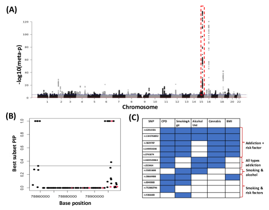
Figure 4: Real data analysis results. (A) Manhattan plot of meta-analyzed p-value from GWAS on each trait. (B) Selection results by our method, y-axis is the best subset PIP, x-axis is the base position and the line denotes the cutoff BFDR$<0.1$ for selecting the causal variants, eQTLs are highlighted in red. (C) The best subset of traits each causal variant targets at, blue box indicates that the corresponding response is selected for that SNP.

SNP	Chromosome	Position	eQTL	Gene	Annotation
rs3829787	15	78563924	No	CHRNA5	intergenic
rs1824520863	15	78565470	No	CHRNA5	-
rs503464	15	78565554	No	CHRNA5	5’UTR
rs55853698	15	78565597	No	CHRNA5	5’UTR
rs752882796	15	78567263	No	CHRNA5	intronic
rs62010331	15	78615354	No	CHRNA3	intronic
rs3743074	15	78617138	No	CHRNA3	intronic
rs28669908	15	78617925	No	CHRNA3	intronic
rs8040868	15	78618839	No	CHRNA3	exonic
rs4366683	15	78619861	No	CHRNA3	intronic
rs149959208	15	78620368	Yes	CHRNA3	intronic
rs1343763852	15	78621646	No	CHRNA3	-

Table 3: The causal variants detected by our method and their annotations

6 Discussion

In this paper, we proposed a novel Bayesian indicator variable selection method that selects predictors at group level, within groups as well as specific to each response for multiple correlated responses with possible heterogeneity. In addition, we proposed a new concept of subset PIP and a permutation-based algorithm to identify the best subset of responses each predictor targets at to facilitate biological findings and generate new hypotheses. We showed that under mild conditions, the posterior median estimators of regression coefficients in our model possess the selection consistency and asymptotic normality. Considering many applications that require the guidance of prior knowledge, we also provided an example of incorporating biological knowledge of eQTL information from existing database in our model to prioritize the selection of causal variants in the context of fine mapping. Via extensive simulation and a real data application to multi-trait fine mapping of multiple addictive behaviors, we showed a remarkable improvement of variable selection performance of our method as compared to other multivariate Bayesian variable selection, regularization and fine-mapping methods.

Nowadays, it is frequent for researchers to collect high-dimensional data on multiple related responses with the aim of identifying the common predictors jointly predictive of these responses from a large pool of candidates. A majority of modern variable selection methods, including both Bayesian variable selection and regularization methods, mainly target at a single response. Running variable selection for each response separately tends to ignore the correlation among responses and is less powerful. The very few options of methods that target at multivariate responses (Liquet et al.,, 2017; Peng et al.,, 2010; Li et al.,, 2015) treat all responses as a whole without considering the heterogeneity across the responses, where each predictor might target at a different subset of responses. This is fairly common phenomenon when we jointly analyze multiple responses from one resource or from multiple studies (Ma et al.,, 2020). Our method is the first Bayesian variable selection method that targets at the multivariate response heterogeneity issue by selecting predictors at multiple levels: group-level, individual feature level and response level, coupled with the best subset of response selection for each predictor. Built on the basis of the more flexible indicator variable selection, our method is easily extensible to handle more complex multi-to-multi problems, e.g. when both predictors and responses have structural patterns. In addition, it is also flexible to put priors on the hyperparameters of selection probabilities in our model to favor selection of certain predictors or certain predictor-response pairs based on existing knowledge, e.g. regulation of gene by miRNA based on motif match from existing sequence database.

In its current implementation and application, our method only considers a relatively fewer number of responses thus we assume a noninformative inverse-wishart prior on the covariance matrix. In the case with a large number of responses with the same level as the number of predictors (Ke et al.,, 2022), priors to encourage simultaneous selection of regression coefficients and covariance terms are strongly recommended (Deshpande et al.,, 2019; Li et al.,, 2021).

We built our model on individual level (raw) genotype data, rather than GWAS summary statistics as in many fine mapping methods. This allows for a more generalizable model that may be applied to many different applications outside fine mapping. Our current application focuses on continuous outcomes, but the model is readily extensible to analyze outcomes of other data types, such as binary, count or mixed data types. Detailed performance will be evaluated in future studies.

The computing time for the real data example of fine mapping for multiple addictive behaviors is 30 mins for 10,000 MCMC iterations with 16 CPU cores, 2.7 GHz and 128 GB RAM. Optimization of code in C++ and applying further parallel computing will likely further reduce computing time (Scott et al.,, 2016; Biswas et al.,, 2022). An efficient R package called ”MBIVS” and data used in this study are available on github at https://github.com/tacanida/MBIVS.

References

- Albert and Chib, (1993) Albert, J. H. and Chib, S. (1993). Bayesian analysis of binary and polychotomous response data. Journal of the American statistical Association, 88(422):669–679.
- Bierut et al., (2008) Bierut, L. J., Stitzel, J. A., Wang, J. C., Hinrichs, A. L., Grucza, R. A., Xuei, X., Saccone, N. L., Saccone, S. F., Bertelsen, S., Fox, L., et al. (2008). Variants in nicotinic receptors and risk for nicotine dependence. American Journal of Psychiatry, 165(9):1163–1171.
- Biswas et al., (2022) Biswas, N., Mackey, L., and Meng, X.-L. (2022). Scalable spike-and-slab. In International Conference on Machine Learning, pages 2021–2040. PMLR.
- Borenstein et al., (2010) Borenstein, M., Hedges, L. V., Higgins, J. P., and Rothstein, H. R. (2010). A basic introduction to fixed-effect and random-effects models for meta-analysis. Research synthesis methods, 1(2):97–111.
- Cano-Gamez and Trynka, (2020) Cano-Gamez, E. and Trynka, G. (2020). From gwas to function: using functional genomics to identify the mechanisms underlying complex diseases. Frontiers in genetics, 11:424.
- Casella et al., (2010) Casella, G., Ghosh, M., Gill, J., and Kyung, M. (2010). Penalized regression, standard errors, and bayesian lassos. Bayesian analysis, 5(2):369–411.
- Cathie et al., (2015) Cathie, S., John, G., Naomi, A., Valerie, B., Paul, B., John, D., Paul, D., Paul, E., Jane, G., Martin, L., Bette, L., Paul, M., Giok, O., Jill, P., Alan, S., Alan, Y., Tim, S., Tim, P., and Rory, C. (2015). Uk biobank: An open access resource for identifying the causes of a wide range of complex diseases of middle and old age. PLOS Medicine, 12(3).
- Chen et al., (2012) Chen, L.-S., Xian, H., Grucza, R. A., Saccone, N. L., Wang, J. C., Johnson, E. O., Breslau, N., Hatsukami, D., and Bierut, L. J. (2012). Nicotine dependence and comorbid psychiatric disorders: examination of specific genetic variants in the chrna5-a3-b4 nicotinic receptor genes. Drug and alcohol dependence, 123:S42–S51.
- Chen et al., (2016) Chen, R.-B., Chu, C.-H., Yuan, S., and Wu, Y. N. (2016). Bayesian sparse group selection. Journal of Computational and Graphical Statistics, 25(3):665–683.
- Consortium et al., (2015) Consortium, G., Ardlie, K. G., Deluca, D. S., Segrè, A. V., Sullivan, T. J., Young, T. R., Gelfand, E. T., Trowbridge, C. A., Maller, J. B., Tukiainen, T., et al. (2015). The genotype-tissue expression (gtex) pilot analysis: multitissue gene regulation in humans. Science, 348(6235):648–660.
- Deshpande et al., (2019) Deshpande, S. K., Ročková, V., and George, E. I. (2019). Simultaneous variable and covariance selection with the multivariate spike-and-slab lasso. Journal of Computational and Graphical Statistics, 28(4):921–931.
- Erzurumluoglu et al., (2020) Erzurumluoglu, A. M., Liu, M., Jackson, V. E., Barnes, D. R., Datta, G., Melbourne, C. A., Young, R., Batini, C., Surendran, P., Jiang, T., et al. (2020). Meta-analysis of up to 622,409 individuals identifies 40 novel smoking behaviour associated genetic loci. Molecular psychiatry, 25(10):2392–2409.
- Fang et al., (2018) Fang, Z., Ma, T., Tang, G., Zhu, L., Yan, Q., Wang, T., Celedón, J. C., Chen, W., and Tseng, G. C. (2018). Bayesian integrative model for multi-omics data with missingness. Bioinformatics, 34(22):3801–3808.
- Farhad et al., (2014) Farhad, H., Emrah, K., Yong, K. E., Bogdan, P., and Eleazar, E. (2014). Identifying causal variants at loci with multiple signals of association. Genetics, 198(2):497–508.
- George and McCulloch, (1993) George, E. I. and McCulloch, R. E. (1993). Variable selection via gibbs sampling. Journal of the American Statistical Association, 88(423):881–889.
- Han and Wei, (2013) Han, F. and Wei, P. (2013). A composite likelihood approach to latent multivaraite gaussian modeling of snp data with application to genetic association testing. Biometrics, 68(1):307–315.
- Harrow et al., (2012) Harrow, J., Frankish, A., Gonzalez, J. M., Tapanari, E., Diekhans, M., Kokocinski, F., Aken, B. L., Barrell, D., Zadissa, A., Searle, S., et al. (2012). Gencode: the reference human genome annotation for the encode project. Genome research, 22(9):1760–1774.
- Hernández-Lobato et al., (2013) Hernández-Lobato, D., Hernández-Lobato, J. M., Dupont, P., et al. (2013). Generalized spike-and-slab priors for bayesian group feature selection using expectation propagation. Journal of Machine Learning Research.
- Hormozdiari et al., (2016) Hormozdiari, F., Van De Bunt, M., Segre, A. V., Li, X., Joo, J. W. J., Bilow, M., Sul, J. H., Sankararaman, S., Pasaniuc, B., and Eskin, E. (2016). Colocalization of gwas and eqtl signals detects target genes. The American Journal of Human Genetics, 99(6):1245–1260.
- Ishwaran and Rao, (2005) Ishwaran, H. and Rao, J. S. (2005). Spike and slab variable selection: frequentist and bayesian strategies. The Annals of Statistics, 33(2):730–773.
- Johnstone and Silverman, (2004) Johnstone, I. M. and Silverman, B. W. (2004). Needles and straw in haystacks: Empirical bayes estimates of possibly sparse sequences. The Annals of Statistics, 32(4):1594–1649.
- Ke et al., (2022) Ke, H., Ren, Z., Qi, J., Chen, S., Tseng, G. C., Ye, Z., and Ma, T. (2022). High-dimension to high-dimension screening for detecting genome-wide epigenetic and noncoding rna regulators of gene expression. Bioinformatics, 38(17):4078–4087.
- Kichaev et al., (2017) Kichaev, G., Roytman, M., Johnson, R., Eskin, E., Lindstroem, S., Kraft, P., and Pasaniuc, B. (2017). Improved methods for multi-trait fine mapping of pleiotropic risk loci. Bioinformatics, 33(2):248–255.
- Kichaev et al., (2014) Kichaev, G., Yang, W.-Y., Lindstrom, S., Hormozdiari, F., Eskin, E., Price, A. L., Kraft, P., and Pasaniuc, B. (2014). Integrating functional data to prioritize causal variants in statistical fine-mapping studies. PLoS genetics, 10(10):e1004722.
- Kruschke, (2014) Kruschke, J. (2014). Doing bayesian data analysis: A tutorial with r, jags, and stan.
- Kuo and Mallick, (1998) Kuo, L. and Mallick, B. (1998). Variable selection for regression models. Sankhyā: The Indian Journal of Statistics, Series B, pages 65–81.
- Li and Tseng, (2011) Li, J. and Tseng, G. C. (2011). An adaptively weighted statistic for detecting differential gene expression when combining multiple transcriptomic studies. Annals of Applied Statistics.
- Li et al., (2021) Li, Y., Datta, J., Craig, B. A., and Bhadra, A. (2021). Joint mean–covariance estimation via the horseshoe. Journal of Multivariate Analysis, 183:104716.
- Li et al., (2015) Li, Y., Nan, B., and Zhu, J. (2015). Multivariate sparse group lasso for the multivariate multiple linear regression with an arbitrary group structure. Biometrics, 71(2):354–363.
- Liquet et al., (2017) Liquet, B., Mengersen, K., Pettitt, A., and Sutton, M. (2017). Bayesian variable selection regression of multivariate responses for group data. Bayesian Analysis, 12(4):1039–1067.
- Liu et al., (2019) Liu, M., Jiang, Y., Wedow, R., Li, Y., Brazel, D. M., Chen, F., Datta, G., Davila-Velderrain, J., McGuire, D., Tian, C., et al. (2019). Association studies of up to 1.2 million individuals yield new insights into the genetic etiology of tobacco and alcohol use. Nature genetics, 51(2):237–244.
- Ma et al., (2020) Ma, T., Ren, Z., and Tseng, G. C. (2020). Variable screening with multiple studies. Statistica Sinica, 30(2):925–953.
- Mitchell and Beauchamp, (1988) Mitchell, T. J. and Beauchamp, J. J. (1988). Bayesian variable selection in linear regression. Journal of the american statistical association, 83(404):1023–1032.
- Newton et al., (2004) Newton, M., Noueiry, A., Sarkar, D., and Ahlquist, P. (2004). Detecting differential gene expression with a semiparametric hierarchical mixture method. Biostatistics, 5(2):155–176.
- Nicolae et al., (2010) Nicolae, D. L., Gamazon, E., Zhang, W., Duan, S., Dolan, M. E., and Cox, N. J. (2010). Trait-associated snps are more likely to be eqtls: annotation to enhance discovery from gwas. PLoS genetics, 6(4):e1000888.
- O’Hara and Sillanpää, (2009) O’Hara, R. B. and Sillanpää, M. J. (2009). A review of bayesian variable selection methods: what, how and which. Bayesian analysis, 4(1):85–117.
- Paaby and Rockman, (2013) Paaby, A. B. and Rockman, M. V. (2013). The many faces of pleiotropy. Trends in genetics, 29(2):66–73.
- Park and Casella, (2008) Park, T. and Casella, G. (2008). The bayesian lasso. Journal of the American Statistical Association, 103(482):681–686.
- Peng et al., (2010) Peng, J., Zhu, J., Bergamaschi, A., Han, W., Noh, D.-Y., Pollack, J. R., and Wang, P. (2010). Regularized multivariate regression for identifying master predictors with application to integrative genomics study of breast cancer. The annals of applied statistics, 4(1):53.
- Quach et al., (2020) Quach, B. C., Bray, M. J., Gaddis, N. C., Liu, M., Palviainen, T., Minica, C. C., Zellers, S., Sherva, R., Aliev, F., Nothnagel, M., et al. (2020). Expanding the genetic architecture of nicotine dependence and its shared genetics with multiple traits. Nature communications, 11(1):5562.
- Saunders et al., (2022) Saunders, G. R., Wang, X., Chen, F., Jang, S.-K., Liu, M., Wang, C., Gao, S., Jiang, Y., Khunsriraksakul, C., Otto, J. M., et al. (2022). Genetic diversity fuels gene discovery for tobacco and alcohol use. Nature, 612(7941):720–724.
- Schaid et al., (2018) Schaid, D. J., Chen, W., and Larson, N. B. (2018). From genome-wide associations to candidate causal variants by statistical fine-mapping. Nature Reviews Genetics, 19(8):491–504.
- Scott et al., (2016) Scott, S. L., Blocker, A. W., Bonassi, F. V., Chipman, H. A., George, E. I., and McCulloch, R. E. (2016). Bayes and big data: The consensus monte carlo algorithm. International Journal of Management Science and Engineering Management, 11(2):78–88.
- Sillanpää and Bhattacharjee, (2005) Sillanpää, M. J. and Bhattacharjee, M. (2005). Bayesian association-based fine mapping in small chromosomal segments. Genetics, 169(1):427–439.
- Sillanpää and Bhattacharjee, (2006) Sillanpää, M. J. and Bhattacharjee, M. (2006). Association mapping of complex trait loci with context-dependent effects and unknown context variable. Genetics, 174(3):1597–1611.
- Simon et al., (2013) Simon, N., Friedman, J., Hastie, T., and Tibshirani, R. (2013). A sparse-group lasso. Journal of computational and graphical statistics, 22(2):231–245.
- Stephens, (2013) Stephens, M. (2013). A unified framework for association analysis with multiple related phenotypes. PloS one, 8(7):e65245.
- Tibshirani, (1996) Tibshirani, R. (1996). Regression shrinkage and selection via the lasso. Journal of the Royal Statistical Society: Series B (Methodological), 58(1):267–288.
- Wang et al., (2020) Wang, G., Sarkar, A., Carbonetto, P., and Stephens, M. (2020). A simple new approach to variable selection in regression, with application to genetic fine-mapping. BioRxiv, page 501114.
- Wang et al., (2009) Wang, J., Grucza, R., Cruchaga, C., Hinrichs, A., Bertelsen, S., Budde, J., Fox, L., Goldstein, E., Reyes, O., Saccone, N., et al. (2009). Genetic variation in the chrna5 gene affects mrna levels and is associated with risk for alcohol dependence. Molecular psychiatry, 14(5):501–510.
- Wang et al., (2007) Wang, T., Zhu, X., and Elston, R. C. (2007). Improving power in contrasting linkage-disequilibrium patterns between cases and controls. The American Journal of Human Genetics, 80(5):911–920.
- Wills et al., (2017) Wills, A. G., Evans, L. M., and Hopfer, C. (2017). Phenotypic and genetic relationship between bmi and drinking in a sample of uk adults. Behavior genetics, 47:290–297.
- Wills and Hopfer, (2019) Wills, A. G. and Hopfer, C. (2019). Phenotypic and genetic relationship between bmi and cigarette smoking in a sample of uk adults. Addictive behaviors, 89:98–103.
- Xu and Ghosh, (2015) Xu, X. and Ghosh, M. (2015). Bayesian variable selection and estimation for group lasso. Bayesian Analysis, 10(4):909–936.
- Yuan and Lin, (2006) Yuan, M. and Lin, Y. (2006). Model selection and estimation in regression with grouped variables. Journal of the Royal Statistical Society: Series B (Statistical Methodology), 68(1):49–67.
- Zhang et al., (2014) Zhang, L., Baladandayuthapani, V., Mallick, B. K., Manyam, G. C., Thompson, P. A., Bondy, M. L., and Do, K.-A. (2014). Bayesian hierarchical structured variable selection methods with application to molecular inversion probe studies in breast cancer. Journal of the Royal Statistical Society: Series C (Applied Statistics), 63(4):595–620.
- Zhao et al., (2019) Zhao, B., Ibrahim, J. G., Li, Y., Li, T., Wang, Y., Shan, Y., Zhu, Z., Zhou, F., Zhang, J., Huang, C., et al. (2019). Heritability of regional brain volumes in large-scale neuroimaging and genetic studies. Cerebral Cortex, 29(7):2904–2914.
- Zhao et al., (2021) Zhao, B., Li, T., Yang, Y., Wang, X., Luo, T., Shan, Y., Zhu, Z., Xiong, D., Hauberg, M. E., Bendl, J., et al. (2021). Common genetic variation influencing human white matter microstructure. Science, 372(6548):eabf3736.
- Zhu et al., (2019) Zhu, L., Huo, Z., Ma, T., Oesterreich, S., and Tseng, G. C. (2019). Bayesian indicator variable selection to incorporate hierarchical overlapping group structure in multi-omics applications. The Annals of Applied Statistics, 13(4):2611–2636.
- Zou and Hastie, (2005) Zou, H. and Hastie, T. (2005). Regularization and variable selection via the elastic net. Journal of the royal statistical society: series B (statistical methodology), 67(2):301–320.