On phase at a resonance in slow-fast Hamiltonian systems

Abstract

We consider a slow-fast Hamiltonian system with one fast angular variable (a fast phase) whose frequency vanishes on some surface in the space of slow variables (a resonant surface). Systems of such form appear in the study of dynamics of charged particles in inhomogeneous magnetic field under influence of a high-frequency electrostatic waves. Trajectories of the averaged over the fast phase system cross the resonant surface. The fast phase makes $\sim\frac{1}{\varepsilon}$ turns before arrival to the resonant surface ($\varepsilon$ is a small parameter of the problem). An asymptotic formula for the value of the phase at the arrival to the resonance was derived earlier in the context of study of charged particle dynamics on the basis of heuristic considerations without any estimates of its accuracy. We provide a rigorous derivation of this formula and prove that its accuracy is $O(\sqrt{\varepsilon})$ (up to a logarithmic correction). Numerics indicate that this estimate for the accuracy is optimal.

1 Introduction

Slow-fast dynamical systems are systems that contain a small parameter, say, $\varepsilon$, and variables of two types: slow, changing with a rate $\sim\varepsilon$, and fast, changing with a rate $\sim 1$. Usually, the dynamics of slow variables is of the principal interest. However, there are systems such that the character of the slow dynamics is determined by the dynamics of fast variables. In particular, this is the case when fast variables are angular variables (rotating phases). Frequencies of rotation of fast phases depend on slow variables. Evolution of the values of slow variables leads to passages through resonances between these frequencies. Passage through a single resonance leads to a jump in the values of slow variables, and the value of this jump depends on a certain linear combination of the values of the phases ([8, 10], see also [13] and references therein). The frequency of this combination of the phases vanishes at the considered resonance. This combination of the phases can be chosen as a new phase for the study of the dynamics near the considered resonance. Thus, the underlying phenomenon is a jump of slow variables when the frequency of one of the phases vanishes on some surface in the space of slow variables (a resonant surface). In this paper we consider a model problem when in a slow-fast Hamiltonian system there is just one fast phase. The frequency of this phase vanishes at some surface in the space of slow variables. This is the resonance in the considered problem. An asymptotic formula that expresses the value of the phase at the resonance via initial conditions taken far from the resonance was suggested in the Appendix to [4] on the basis of a heuristic consideration without an estimate of the accuracy of this formula. In the current paper we present a rigorous derivation of this formula with an estimate of its accuracy. Phase at a resonance in systems with dissipation is discussed in [6], [11].

Systems of the considered form appear, in particular, in the study of dynamics of charged particles in inhomogeneous magnetic field under influence of a high-frequency electrostatic wave ([4] and references therein). The fast phase in these problems is the phase of the wave. The resonance occurs when the projection of the velocity of the particle onto the direction of wave propagation is equal to the phase velocity of the wave. Passage through this resonance leads to a jump in the particle energy. The value of this jump depends on the phase of the wave at the resonance. The formula for this phase together with the formula for the jump of energy are used in [4] to derive a map describing the changes of the energy of the particle and the phase of the wave for consecutive passages through the resonance. The iterations of this map are used in [4] to model the long-term dynamics of particles with multiple passages through the resonance. Such an approach allows for a drastic reduction of the modelling time in comparison with direct tracking of particles trajectories by solving the differential equations of the motion numerically.

The structure of this paper is as follows. In Section 2 we state the considered problem. The required assumptions are formulated in Section 3. The main result of the paper, the formula for the phase at a resonance (Theorem 1) is stated in Section 4. The rest of the paper contains the proof of this formula. In the Appendix we discuss a probabilistic aspect of the problem.

2 Outline of the problem

We consider a slow-fast Hamiltonian system with two pairs of canonically conjugate variables $(I,\varphi)$, $(\varepsilon^{-1}x,y)$ and a Hamilton’s function

$$H(I,\varphi,y,x,\varepsilon)=H_{0}(I,y,x)+\varepsilon H_{1}(I,\varphi,y,x,\varepsilon).$$ (2.1)

Here $\varepsilon>0$ is a small parameter of the problem, $I\in\mathbb{R}$, $\varphi\in{\mathbb{S}}^{1}$, $(y,x)\in\mathbb{R}^{2n},\ n\geq 1$, and $H_{1}$ is $2\pi$-periodic in $\varphi$. The variables $I$ and $\varphi$ are called the action variable and the angle variable (respectively) of this system. The angle variable is also called the phase. The corresponding differential equations are

$$\dot{I} =-\varepsilon\frac{\partial H_{1}}{\partial\varphi},\quad\dot{\varphi}=\frac{\partial H_{0}}{\partial I}+\varepsilon\frac{\partial H_{1}}{\partial I},$$ (2.2)

$$\dot{y} =-\varepsilon\frac{\partial H_{0}}{\partial x}-\varepsilon^{2}\frac{\partial H_{1}}{\partial x},\quad\dot{x}=\varepsilon\frac{\partial H_{0}}{\partial y}+\varepsilon^{2}\frac{\partial H_{1}}{\partial y}\,.$$

Thus, $I,y,x$ are slow variables, and $\varphi$ is a fast variable (the fast phase). The function

$$\omega_{0}(I,y,x)=\frac{\partial H_{0}(I,y,x)}{\partial I}$$ (2.3)

is the frequency of the fast phase. We assume that this frequency vanishes on some surface ${\cal R}$ in the space of slow variables. This surface will be called the resonant surface.

For an approximate description of the behaviour of the slow variables one can use the averaged system [5]. In the considered case the averaged system has the following simple form

$$\dot{\bar{I}}=0,\quad\dot{\bar{y}}=-\varepsilon\frac{\partial H_{0}(\bar{I},\bar{y},\bar{x})}{\partial x},\quad\dot{\bar{x}}=\varepsilon\frac{\partial H_{0}(\bar{I},\bar{y},\bar{x})}{\partial y}\,.$$ (2.4)

Thus, for the variables $\bar{y},\bar{x}$ considered as canonically conjugate variables we have a Hamiltonian system with the Hamiltonian $\varepsilon H_{0}(\bar{I},\bar{y},\bar{x})$ that depends on the parameter $\bar{I}={\rm const}$. An approximation provided by these formulas is called an adiabatic approximation, the variable $I$ is an adiabatic invariant.

Consider a solution $(I(t),\varphi(t),y(t),x(t))$ of the system (2.2) with the initial data $(I_{0},\varphi_{0},y_{0},x_{0})$ at $t=t_{0}$. Consider the solution $(\bar{I},\bar{y}(\tau),\bar{x}(\tau))$ of the averaged system (2.4) with the same initial condition for slow variables: $\bar{I}=I_{0}$, $\bar{y}(\tau_{0})=y_{0}$, $\bar{x}(\tau_{0})=x_{0}$. Here we have introduced the slow time $\tau=\varepsilon t$, and $\tau_{0}=\varepsilon t_{0}$. Assume that the considered solution of the averaged system arrives to the resonant surface for the first time at a moment of slow time $\tau_{*}$. Then, if some mild conditions are satisfied, the considered solution of the exact system also arrives to the resonant surface, suppose that this happens for $t=t_{e}$. The value of $\varepsilon t_{e}=\tau_{e}$ is close to $\tau_{*}$. Let $\varphi_{e}$ denote the value of the fast phase at the resonance, $\varphi_{e}=\varphi(t_{e})$. The goal of this paper is to provide a rigorous derivation of an asymptotic formula for the value $\varphi_{e}$ and obtain an estimate of its accuracy.

3 Formulation of assumptions

System (2.2) is considered for $(I,y,x,\varphi)\in D\times\mathbb{S}^{1}$, $0\leq\varepsilon\leq\varepsilon_{1}$, where $D$ is a compact domain, $\varepsilon_{1}={\rm const}$. Solutions of system (2.2) are considered for initial conditions in the domain $D_{0}\times\mathbb{S}^{1}$, where $D_{0}$ is a compact domain with a piece-wise smooth boundary, $D_{0}\subset D$. We assume that the following conditions are satisfied.

1. Functions $H_{0},H_{1}$ are three times continuously differentiable in $I,\varphi,y,x$. Function $H_{1}$ is one time continuously differentiable in $\varepsilon$.

2. Function $H_{0}$ is non-degenerate on the resonant surface ${\cal R}$:

   $$\frac{\partial^{2}H_{0}(I,y,x)}{\partial I^{2}}\equiv\frac{\partial\omega_{0}(I,y,x)}{\partial I}\neq 0\ {\rm at}\ (I,y,x)\in{\cal R}.$$ (3.1)

3. Solutions of the averaged system cross the resonant surface ${\cal R}$ transversally:

   $$\frac{\partial\omega_{0}(I,y,x)}{\partial x}\frac{\partial H_{0}(I,y,x)}{\partial y}-\frac{\partial\omega_{0}(I,y,x)}{\partial y}\frac{\partial H_{0}(I,y,x)}{\partial x}\neq 0\ {\rm at}\ (I,y,x)\in{\cal R}.$$ (3.2)

4. Solutions of the averaged system with initial conditions in $D_{0}$ are well defined, stay at a positive distance from the boundary of $D$ for $\tau_{0}\leq\tau\leq\tau_{0}+K,\;K={\rm const}>0$, and cross the resonant surface ${\cal R}$ at some $\tau=\tau_{*}\in(\tau_{0},\tau_{0}+K),\;y=y_{*},\;x=x_{*}$.

Condition B) implies that the equation of the resonant surface can be presented in the form $I=a(y,x)$ with some smooth function $a(y,x)$. Then $\omega_{0}(a(y,x),y,x)\equiv 0$. Denote

$$\alpha(y,x) = \frac{\partial^{2}H_{0}(a(y,x),y,x)}{\partial I^{2}},$$ (3.3)

$$b(y,x) = \frac{\partial a(y,x)}{\partial x}\frac{\partial H_{0}(a(y,x),y,x)}{\partial y}-\frac{\partial a(y,x)}{\partial y}\frac{\partial H_{0}(a(y,x),y,x)}{\partial x}.$$ (3.4)

Condition B) implies that $\alpha(y,x)\neq 0$. Condition C) implies that $b(y,x)\neq 0$.

For the sake of being definite assume that $\alpha(y,x)>0$, that $I>a(y,x)$ in the domain $\omega_{0}(I,y,x)>0$, and that $b(y,x)>0$. Then condition C) implies that we should consider the motion that starts at the domain $\omega_{0}>0$, i.e. $I_{0}>a(y_{0},x_{0})$.

The following function is important in dynamics near the resonance:

$$F(\varphi,y,x)=b(y,x)\varphi+H_{1}(a(y,x),\varphi,y,x,0).$$ (3.5)

We will assume that the following genericity condition is satisfied (its origin is explained in Section 5).

1. All critical points of the function $F$, considered as a function of $\varphi$, are non-degenerate: if $\frac{\partial F}{\partial\varphi}=0$ at some point, then $\frac{\partial^{2}F}{\partial\varphi^{2}}\neq 0$ at this point. Moreover, the values of $F$ at the critical points are different from each other.

Note that if $F$ does not have critical points, this condition is satisfied.

Proposition 1

Fix any number $r>1$. If the initial condition for a solution of system (2.2) does not belong to some exceptional set ${\cal V}_{r}$ of measure $O(\varepsilon^{r})$, then this solution crosses the resonan surface at some moment $\tau_{e}$ of the slow time and at a value $\varphi_{e}$ of the phase. Moreover, $\tau_{e}=\tau_{*}+O(\sqrt{\varepsilon}\ln\nu)$, where $\nu=\min(\frac{1}{2},\nu_{1}+\varepsilon)$, and $\nu_{1}>0$ is the minimum of distances of $\varphi_{e}$ from the points of local maximum of the function $F(\varphi,y_{*},x_{*})$. If this function does not have critical points, then ${\cal V}_{r}$ is empty and $\tau_{e}=\tau_{*}+O(\sqrt{\varepsilon})$.

Here $r>0$ can be taken arbitrary large, but the constant in the symbol $O(\sqrt{\varepsilon}\ln\nu)$ depends on the choice of $r$. Proposition 1 is a direct corollary of Lemma 6.2 formulated in Section 6.2.

4 Formula for phase at the resonance

The second approximation of the averaging method is routinely used to approximately describe how the phase depends on the time far from resonances. It works on time intervals $\sim\frac{1}{\varepsilon}$ with accuracy $o(1)$ (see, e.g., [5]). To apply the second-order averaging for the considered system, one should introduce new variables $(J,\psi,\eta,\xi)$ that are related to the old variables $(I,\varphi,y,x)$ via the canonical transformation of variables with the generating function

$$W(J,\varphi,\eta,x,\varepsilon)=J\varphi+\varepsilon^{-1}\eta x+\varepsilon S_{1}(J,\varphi,\eta,x).$$ (4.1)

Old and new variables are related as follows:

$$I=J+\varepsilon\frac{\partial S_{1}(J,\varphi,\eta,x)}{\partial\varphi},\quad\psi=\varphi+\varepsilon\frac{\partial S_{1}(J,\varphi,\eta,x)}{\partial J},$$ (4.2)

$$y=\eta+\varepsilon^{2}\frac{\partial S_{1}(J,\varphi,\eta,x)}{\partial x},\quad\xi=x+\varepsilon^{2}\frac{\partial S_{1}(J,\varphi,\eta,x)}{\partial\eta}.$$

Let

$${\cal H}_{1}(I,y,x)=\frac{1}{2\pi}\int_{0}^{2\pi}H_{1}(I,\varphi,y,x,0)d\varphi$$

denote the average of the function $H_{1}$ over the fast phase at $\varepsilon=0$. The function $S_{1}$ is uniquely defined by the formula

$$\frac{\partial S_{1}(I,\varphi,y,x)}{\partial\varphi}=\frac{1}{\omega_{0}(I,y,x)}\left[{\cal H}_{1}(I,y,x)-H_{1}(I,\varphi,y,x,0)\right]$$ (4.3)

and the condition that the average of $S_{1}(I,\varphi,y,x)$ over $\varphi$ is equal to 0.

The dynamics of the variables $J,\psi,\eta,\xi$ is approximately described by the Hamiltonian system with Hamilton’s function

$${\cal H}_{a}(J,\eta,\xi,\varepsilon)=H_{0}(J,\eta,\xi)+\varepsilon{\cal H}_{1}(J,\eta,\xi).$$ (4.4)

The corresponding differential equations are

$$\dot{J} = 0,\quad\dot{\eta}=-\varepsilon\frac{\partial{\cal H}_{a}(J,\eta,\xi,\varepsilon)}{\partial\xi},\quad\dot{\xi}=\varepsilon\frac{\partial{\cal H}_{a}(J,\eta,\xi,\varepsilon)}{\partial\eta},$$ (4.5)

$$\dot{\psi} = \frac{\partial{\cal H}_{a}(J,\eta,\xi,\varepsilon)}{\partial J}.$$

Thus, for the variables $\eta,\xi$ we have a Hamiltonian system with the Hamiltonian $\varepsilon{\cal H}_{a}(J,\eta,\xi,\varepsilon)$ that depends on the parameter $J={\rm const}$. Initial condition $(J_{0},\eta_{0},\xi_{0})$ for this system should be obtained from the initial condition $(I_{0},\varphi_{0},y_{0},x_{0})$ of the system (2.2) using the transformation of variables (4.2). An approximation provided by these formulas is called an improved adiabatic approximation, the variable $J$ is an improved adiabatic invariant.

Denote

$$\omega_{1}(I,y,x)=\frac{\partial{\cal H}_{1}(I,y,x)}{\partial I}.$$ (4.6)

The frequency of the phase $\psi$ in the system (4.5) is $\omega_{0}(J,\eta,\xi)+\varepsilon\omega_{1}(J,\eta,\xi)$.

Denote by $\tilde{H}_{1}(I,\varphi,y,x)$ the purely periodic (i.e. with average 0) part of $H_{1}(I,\varphi,y,x,0)$. Then $\tilde{H}_{1}(I,\varphi,y,x)=H_{1}(I,\varphi,y,x,0)-{\cal H}_{1}(I,y,x)$. Denote

$$\Xi=\frac{1}{2\pi}\left(\varphi_{e}+\frac{\tilde{H}_{1}(I_{0},\varphi_{e},y_{*},x_{*})}{b(y_{*},x_{*})}\right).$$ (4.7)

Denote by $J_{0},\eta_{a}(\tau),\xi_{a}(\tau)$ the solution of the differential equations (4.5) for $J,\eta,\xi$ with initial condition $(J_{0},\eta_{0},\xi_{0})$. Denote by $\tau_{*,a}$ the moment of the slow time when this solution crosses the resonant surface: $a(\eta_{a}(\tau_{*,a}),\xi_{a}(\tau_{*,a}))=J_{0}$.

Theorem 1

If the initial point $(I_{0},\varphi_{0},y_{0},x_{0})$ does not belong to the exceptional set ${\cal V}_{r}$, then the following asymptotic formula for $\Xi$ is valid:

$$2\pi\Xi= \varphi_{0}+\frac{1}{\varepsilon}\int_{\tau_{0}}^{\tau_{*,a}}\left(\omega_{0}(J_{0},\eta_{a}(\tau),\xi_{a}(\tau))+\varepsilon\omega_{1}(J_{0},\eta_{a}(\tau),\xi_{a}(\tau)\right)d\tau+O(\sqrt{\varepsilon}\ln\nu).$$ (4.8)

Here the objects $r,{\cal V}_{r},\nu$ are those introduced in Proposition 1 and are associated with points of local maximum of the function $F(\varphi,y_{*},x_{*})$. If $F$ does not have critical points, then ${\cal V}_{r}$ is empty and $\nu=1/2$, i.e. the error term in (4.8) is $O(\sqrt{\varepsilon})$.

This theorem is the main result of the paper. It is proven in Section 7 on the basis of some preliminary estimates and constructions contained in Sections 5, 6. Proofs of the preliminary estimates and auxiliary lemmas are given in Sections 9, 10.

Remark. Theorem 1 does not describe initial conditions that belong to the exceptional set ${\cal V}_{r}$. However, this theorem determines which initial conditions are guaranteed to be outside ${\cal V}_{r}$. Let $\varphi_{j},j=1,2,\ldots,k$, be points of maximum of the function $F(\varphi,y_{*},x_{*})$ on the interval $[0,2\pi)$. Denote $\tilde{F}$ the purely periodic part of the function $F$. Denote $\hat{\Xi}_{j},\,j=1,2,\ldots,k$, fractional parts of values $\tilde{F}(\varphi_{j},y_{*},x_{*})/(2\pi b(y_{*},x_{*}))$. Denote as $\Xi_{a}$ the principal term in expression for $\Xi$ given by (4.8). Let $\hat{\Xi}_{a}$ be the fractional part of $\Xi_{a}$. Then there exists a constant $c_{a}>0$ such that if the initial point $(I_{0},\varphi_{0},y_{0},x_{0})$ is such that the value $\hat{\Xi}_{a}$ is at the distance bigger than $c_{a}\sqrt{\varepsilon}|\ln\varepsilon|$ from each of values $\hat{\Xi}_{j},j=1,2,\ldots,k$, then this initial point does not belong to the exceptional set ${\cal V}_{r}$.

Value $\Xi$ as a characteristic of a passage through resonance was introduced in [13]. It is determined modulo 1 (because the value of phase $\varphi_{e}$ at the resonance is determined modulo $2\pi$). We call $\Xi$ pseudophase in analogy with the terminology used in description of separatrices crossings [16]. The phase at the resonance $\varphi_{e}$ is uniquely determined by the pseudophase $\Xi$. If the function $F$ (3.5), considered as a function of $\varphi$, does not have critical points, then one can solve relation (4.7) for $\varphi_{e}$. Together with Theorem 1 this gives an asymptotic formula for $\varphi_{e}$ with an accuracy $O(\sqrt{\varepsilon}\,)$. If the function $F$ (3.5) has critical points, then $\varphi_{e}$ can’t belong to some intervals (this is explained in Section 5). In this case relation (4.7) should be solved for $\varphi_{e}$ on some intervals of monotonicity of $F$ to get an asymptotic formula for $\varphi_{e}$, see Section 5. The phase $\varphi_{e}$ will be determined with an accuracy $O(\sqrt{\varepsilon}\,)$ far from critical points of $F$. The accuracy decays close to critical points of $F$. It is $O(\varepsilon^{\frac{1}{4}}|\ln\varepsilon|^{1/2})$ when $\Xi$ is $\sqrt{\varepsilon\,}|\ln\varepsilon|$-close to a critical value $\tilde{F}_{c}$ of $\tilde{F}(\varphi,y_{*},x_{*})$ and is $O\left(\cfrac{\sqrt{\varepsilon}\ln|\Xi-\tilde{F}_{c}|}{(\sqrt{|\Xi-\tilde{F}_{c}|}}\right)$ when $|\Xi-\tilde{F}_{c}|>\sqrt{\varepsilon}|\ln\varepsilon|$. (Logarithmic terms can be omitted for $\varphi_{e}$ near a critical point $\varphi_{c}$ of the function $F$ if the phase $\varphi$ is measured from this critical point, i. e., if $\varphi_{c}\equiv 0$.)

The problem of calculation of pseudophase $\Xi\ {\rm mod}\ 1$ (or phase $\varphi_{e}\ {\rm mod}\ 2\pi$) for given initial conditions does not have a deterministic answer in the limit as $\varepsilon\to 0$. However, one can interpret $\hat{\Xi}={\rm Frac}\,(\Xi)$, the fractional part of $\Xi$, as a random value and calculate a limiting probabilistic distribution of this value. Such an approach to a problem with a small parameter was suggested in [12] and then was rediscovered and used by many authors (in particular, in [9]). A rigorous natural definition of what should be called a probability in such problems was suggested in [2]. (There are also other natural definitions. In cases when results of calculation of probabilities using different definitions are known, these results coincide.) According to [13], the value $\hat{\Xi}$ has a uniform distribution on the interval $[0,1]$ in the limit as $\varepsilon\to 0$. This result is obtained by calculation of phase fluxes, without knowledge of asymptotic formula for $\Xi$. Formula (4.8) allows to give an alternative proof of this result (see Appendix).

A general scheme of the proof of Theorem 1 is as follows. Inside $O(\sqrt{\varepsilon})$-neighbourhood of the resonant surface one can use an expansion with respect to the distance from the resonant surface for description of the dynamics. It is known that the obtained “pendulum-like” system has an approximate first integral (cf. Section 5). We introduce an auxiliary function (this is the function $E$ in Section 7) which is close to this first integral near the resonance. Due to this, one can get good estimates of change of this function near the resonance: its change is $O(\sqrt{\varepsilon}\ln\nu)$ or $O(\sqrt{\varepsilon})$ in $\sqrt{\varepsilon}$-neighbourhood of the resonant surface. Outside $\sim\sqrt{\varepsilon}$-neighbourhood of the resonant surface one can make a transformation of variables which excludes fast phase from the Hamiltonian up to a prescribed order in $\varepsilon$. Using such transformations is a standard approach in the averaging method [5]. This allows to calculate the change of function $E$ outside $\sqrt{\varepsilon}$-neighbourhood of the resonance with an accuracy $O(\sqrt{\varepsilon})$. Combining the estimates near and far from the resonance we get an asymptotic formula for change of $E$ from the initial value to arrival into resonance with an accuracy $O(\sqrt{\varepsilon}\ln\nu)$ or $O(\sqrt{\varepsilon})$. This provides an equality that includes value $\Xi$ (4.7). Solving this equality for $\Xi$ gives relation (4.8) in Theorem 1.

5 Expansion near the resonant surface

Study of dynamics close to resonance can be reduced to study of behaviour of a perturbed pendulum-like system. Such a reduction was used in a number of papers starting from [8]; see, e.g., [3] and references therein. We will perform this reduction in a Hamiltonian form following [14].

Expansion of Hamiltonian (2.1) over $(I-a(y,x))$ is

$$H=H_{0}(a(y,x),y,x)+\frac{1}{2}\alpha(y,x)(I-a(y,x))^{2}+\varepsilon H_{1}(a(y,x),\varphi,y,x,0)$$ (5.1)

$$+O((I-a(y,x))^{3})+\varepsilon O(I-a(y,x))+O(\varepsilon^{2}),\phantom{***********}$$

where the function $\alpha$ is given by formula (3.3). Make a canonical transformation of variables $(I,\varphi,y,x)\mapsto(\sqrt{\varepsilon}P,\gamma,\tilde{y},\tilde{x})$ with the generating function

$$W_{res}(P,\varphi,\tilde{y},x,\varepsilon)=\tilde{y}\varepsilon^{-1}x+(\sqrt{\varepsilon}P+a(\tilde{y},x))\varphi.$$ (5.2)

Then $\gamma=\varphi,\ I=\sqrt{\varepsilon}P+a(\tilde{y},\tilde{x})+O(\varepsilon)$. Other old variables are expressed via new ones as follows:

$$y=\tilde{y}+\varepsilon\dfrac{\partial a(\tilde{y},\tilde{x})}{\partial\tilde{x}}\varphi+O(\varepsilon^{2}),\quad x=\tilde{x}-\varepsilon\dfrac{\partial a(\tilde{y},\tilde{x})}{\partial\tilde{y}}\varphi+O(\varepsilon^{2}).$$ (5.3)

Note that in these estimates we assume that $\varphi=O(1)$. The Hamiltonian (2.1) in the new variables takes the form

$$H = H_{0}(a(\tilde{y},\tilde{x}),\tilde{y},\tilde{x})$$

$$+ \varepsilon\left(\frac{1}{2}\alpha(\tilde{y},\tilde{x})P^{2}+b(\tilde{y},\tilde{x})\varphi+H_{1}(a(\tilde{y},\tilde{x}),\varphi,\tilde{y},\tilde{x},0)\right)$$

$$+ \varepsilon^{\frac{3}{2}}O(P^{3})+\varepsilon^{\frac{3}{2}}O(P)+O(\varepsilon^{2}),$$

where the function $b$ is given by formula (3.4). Consider motion in a strip near the resonant surface where $P=O(1)$, and neglect terms $O(\varepsilon^{\frac{3}{2}})$. Introduce the new time $\theta=\sqrt{\varepsilon}t$. For dynamics of $\tilde{y},\tilde{x}$ considered as canonically conjugate variables we get a Hamiltonian system with Hamilton’s function $\sqrt{\varepsilon}\Lambda(\tilde{y},\tilde{x})$, where $\Lambda=H_{0}(a(\tilde{y},\tilde{x}),\tilde{y},\tilde{x})$. Dynamics of $P,\varphi$ in the principal approximation can be considered for frozen $\tilde{y},\tilde{x}$. Then for $P,\varphi$ we get the Hamiltonian system with Hamilton’s function

$${\cal E}(P,\varphi,\tilde{y},\tilde{x})=\frac{1}{2}\alpha(\tilde{y},\tilde{x})P^{2}+b(\tilde{y},\tilde{x})\varphi+H_{1}(a(\tilde{y},\tilde{x}),\varphi,\tilde{y},\tilde{x},0),$$ (5.5)

i.e.

$${\cal E}(P,\varphi,\tilde{y},\tilde{x})=\frac{1}{2}\alpha(\tilde{y},\tilde{x})P^{2}+F(\varphi,\tilde{y},\tilde{x}),$$ (5.6)

where the function $F$ is given by formula (3.5). Here $P,\varphi$ are canonically conjugate variables (note that in (5) canonically conjugate variables are $\sqrt{\varepsilon}P,\varphi$).

Hamiltonian (5.5) describes a one-dimensional motion in $2\pi$-periodic potential $H_{1}(a(\tilde{y},\tilde{x}),\varphi,\tilde{y},\tilde{x},0)$ under the action of the constant torque $b(\tilde{y},\tilde{x})$ (a “pendulum-like system”). There are two types of phase portraits of this Hamiltonian: without oscillatory domains (Fig. 1, a) and with oscillatory domains (Fig. 1, b).

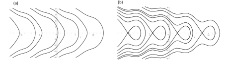
Figure 1: Phase portraits of pendulum-like systems: (a) without oscillatory domains, (b) with oscillatory domains.

Condition E) in Section 3 implies that unstable equilibria in Fig. 1, b are non-degenerate saddles, and that separatrices do not connect different saddles .

If the phase portrait of the Hamiltonian ${\cal E}$ does not have oscillatory domains for $x=x_{*},y=y_{*}$, then the phase at the resonance $\varphi_{e}$ can have any value modulo $2\pi$. To determine an approximate value of $\varphi_{e}$ it is enough to solve the relation (4.7) for $\varphi_{e}$ and use the approximate value for $\Xi$ given by formula (4.8). If there are oscillatory domains, then, in the approximation (5.6), values of $\varphi_{e}$ can’t correspond to points in oscillatory domains. To find $\varphi_{e}$ ${\rm mod}\ 2\pi$, one can solve relation (4.7) on intervals of monotonicity of the function $F$ for $\varphi$ outside oscillatory domains and use the approximate value for $\Xi$ from (4.8). However, due to the perturbation in (5), the point $P=0,\varphi=\varphi_{e}$ can be in an oscillatory domain with value of $\Xi$ which is $O(\sqrt{\varepsilon})$-close to the value of $F(\varphi,y_{*},x_{*})$ at a saddle point on the boundary of this domain.

6 Preliminary estimates

Fix an initial condition $(I_{0},\varphi_{0},y_{0},x_{0})$ at $t=t_{0}$ and the solution $(I(t),\varphi(t),y(t),x(t))$ of system (2.2) with this initial condition. Rewrite these initial conditions and solution in variables $(J,\psi,\eta,\xi)$ introduced by the transformation (4.2). We get an initial condition $(J_{0},\psi_{0},\eta_{0},\xi_{0})$ and solution $(J(t),\psi(t),\eta(t),\xi(t))$. Consider solution $(J_{0},\psi_{a}(\tau),\eta_{a}(\tau),\xi_{a}(\tau))$ of system (4.5) with initial condition $(J_{0},\psi_{0},\eta_{0},\xi_{0})$ at $\tau=\tau_{0}=\varepsilon t_{0}$. Denote $\omega_{a}(\tau)=\omega_{0}(J_{0},\eta_{a}(\tau),\xi_{a}(\tau))$.

6.1 Estimates up to distance $\sim\sqrt{\varepsilon}$ from the resonance

Lemma 6.1

There exists a constant $C_{1}>0$ such that while $\omega_{a}(\tau)\geq C_{1}\sqrt{\varepsilon}$ the solution $(J(t),\psi(t),\eta(t),\xi(t))$ is well defined and the following estimates are satisfied:

$$|J(t)-J_{0}|=O\left(\frac{\varepsilon^{2}}{\omega^{3}_{a}(\tau)}\right),\quad|\psi(t)-\psi_{a}(\tau)|=O\left(\frac{\varepsilon}{\omega^{2}_{a}(\tau)}\right),$$ (6.1)

$$|\eta(t)-\eta_{a}(\tau)|=O\left(\frac{\varepsilon^{2}}{\omega^{2}_{a}(\tau)}\right),\quad|\xi(t)-\xi_{a}(\tau)|=O\left(\frac{\varepsilon^{2}}{\omega^{2}_{a}(\tau)}\right),$$ (6.2)

$$|I(t)-J(t)|=O\left(\frac{\varepsilon}{\omega_{a}(\tau)}\right),\quad|\varphi(t)-\psi(t)|=O\left(\frac{\varepsilon}{\omega^{2}_{a}(\tau)}\right),$$ (6.3)

$$|y(t)-\eta(t)|=O\left(\frac{\varepsilon^{2}}{\omega^{2}_{a}(\tau)}\right),\quad|x(t)-\xi(t)|=O\left(\frac{\varepsilon^{2}}{\omega^{2}_{a}(\tau)}\right),$$ (6.4)

$$\omega_{0}(J(t),\eta(t),\xi(t))>\frac{1}{2}\omega_{a}(\tau),\quad\omega_{0}(I(t),y(t),x(t))>\frac{1}{2}\omega_{a}(\tau).$$ (6.5)

This lemma is proven in Section 9.1.

6.2 Estimates for slow variables up to arrival to resonance

Lemma 6.2

(a) There exist a constant $C_{2}>C_{1}$ and a moment of time $t_{N}$ such that

$$\omega_{0}(I(t_{N}),y(t_{N}),x(t_{N}))=C_{2}\sqrt{\varepsilon},\ \omega_{a}(\varepsilon t_{N})>2C_{1}\sqrt{\varepsilon},\ \varepsilon t_{N}=\tau_{*}+O(\sqrt{\varepsilon}).$$

(b) Fix a number $r>1$. If the initial condition $(I_{0},\varphi_{0},y_{0},x_{0})$ does not belong to an exceptional set ${\cal V}_{r}$ of measure $O(\varepsilon^{r})$, then the solution $(I(t),\varphi(t),y(t),x(t))$ arrives to the resonant surface at some $t=t_{e}$ (i.e. $\omega_{0}(I(t_{e}),y(t_{e}),x(t_{e}))=0$, or, which is the same, $a(y(t_{e}),x(t_{e}))=I(t_{e})$). Denote $\nu=\min(\frac{1}{2},\nu_{1}+\varepsilon)$, where $\nu_{1}>0$ is the minimum of distances of $\varphi(t_{e})$ from the points of maximum of the function $F(\varphi,y_{*},x_{*})$. Then $\varepsilon t_{e}=\tau_{*}+O(\sqrt{\varepsilon}\ln\nu)$. For $t_{N}\leq t\leq t_{e}$ the following estimates are satisfied:

$$I(t) =I_{0}+O(\sqrt{\varepsilon}\ln\nu),$$ (6.6)

$$y(t) =\eta_{a}(\tau)+O(\varepsilon\ln^{2}\nu),\;x(t)=\xi_{a}(\tau)+O(\varepsilon\ln^{2}\nu).$$

(c) If the function $F$ does not have critical points, then for any initial conditions the solution arrives to the resonance surface, and one can omit $\ln\nu$ in the previous estimates, i.e.

$$\varepsilon t_{e} =\tau_{*}+O(\sqrt{\varepsilon}),\ I(t)=I_{0}+O(\sqrt{\varepsilon}),$$ (6.7)

$$y(t) =\eta_{a}(\varepsilon t)+O(\varepsilon),\ x(t)=\xi_{a}(\varepsilon t)+O(\varepsilon).$$

This lemma is proven in Section 9.2.

7 Proof of Theorem 1

We consider solution $(I(t),\varphi(t),y(t),x(t))$ of the system (2.2). We assume that initial condition $(I_{0},\varphi_{0},y_{0},x_{0})$ at $t=t_{0}$ of this solution does not belong to the exceptional set ${\cal V}_{r}$. According to Proposition 1, this solution crosses the resonant surface at some moment of time $t_{e}$. We denote $I_{e}=I(t_{e}),\varphi_{e}=\varphi(t_{e}),y_{e}=y(t_{e}),x_{e}=x(t_{e}),\tau_{0}=\varepsilon t_{0},\tau_{e}=\varepsilon t_{e}$. Crossing the resonance means that $\omega_{0}(I_{e},y_{e},x_{e})=0$ or, equivalently, $a(y_{e},x_{e})=I_{e}$. Without loss of generality we put $t_{0}=0,\tau_{0}=0$. We use prime to denote derivative with respect to $\tau$.

We use notation of previous sections: $(J(t),\psi(t),\eta(t),\xi(t))$ is the solution represented in variables (4.2), $(J_{0},\psi_{0},\eta_{0},\xi_{0})$ is its initial condition, $(J_{0},\psi_{a}(\tau),\eta_{a}(\tau),\xi_{a}(\tau))$ is the solution of system (4.5) with the initial condition $(J_{0},\psi_{0},\eta_{0},\xi_{0})$ at $\tau=0$, and $\omega_{a}(\tau)=\omega_{0}(J_{0},\eta_{a}(\tau),\xi_{a}(\tau))$. There is a moment of the slow time $\tau=\tau_{*,a}$ such that $\omega_{a}(\tau_{*,a})=0$. Proposition 1 implies that $\tau_{e}=\tau_{*,a}+O(\sqrt{\varepsilon}\ln\nu)$.

The expansion of $H_{0}(I,y,x)$ over $(I-a(y,x))$ is

$$H_{0}(I,y,x)=\Lambda(y,x)+\frac{1}{2}\alpha(y,x)(I-a(y,x))^{2}+M(I,y,x),$$ (7.1)

where $M(I,y,x)=O((I-a(y,x))^{3})$. From (2.2) we get

$$\dot{\varphi}=\alpha(y,x)(I-a(y,x))+\frac{\partial M(I,y,x)}{\partial I}+\varepsilon\frac{\partial H_{1}(I,\varphi,y,x,0)}{\partial I}+O(\varepsilon^{2}).$$ (7.2)

Denote

$$B_{0}(I,y,x)= \frac{\partial a(y,x)}{\partial x}\frac{\partial H_{0}(I,y,x)}{\partial y}-\frac{\partial a(y,x)}{\partial y}\frac{\partial H_{0}(I,y,x)}{\partial x}$$

$$= b(y,x)+\frac{\partial a(y,x)}{\partial x}\frac{\partial N(I,y,x)}{\partial y}-\frac{\partial a(y,x)}{\partial y}\frac{\partial N(I,y,x)}{\partial x},$$

$$B_{1}(I,\varphi,y,x)= \frac{\partial a(y,x)}{\partial x}\frac{\partial H_{1}(I,\varphi,y,x,0)}{\partial y}-\frac{\partial a(y,x)}{\partial y}\frac{\partial H_{1}(I,\varphi,y,x,0)}{\partial x},$$

$$b_{*,a} =b(\eta_{a}(\tau_{*,a}),\xi_{a}(\tau_{*,a})),\ N(I,y,x)=O((I-a(y,x))^{2}).$$

Consider the function:

$$E=\frac{1}{2\varepsilon}\alpha(y,x)(I-a(y,x))^{2}+H_{1}(I,\varphi,y,x,\varepsilon)+b_{*,a}\varphi.$$ (7.3)

This function is an approximate first integral of motion in system (2.2) near the resonant surface. Calculate derivative $\dot{E}$ of this function along solution $(I(t),\varphi(t),y(t),x(t))$ and take the integral of this derivative from 0 to $t_{e}$. Compare two expressions of this integral. On the one hand,

$$\int^{t_{e}}_{0}\dot{E}dt=E|_{t=t_{e}}-E|_{t=0}$$ (7.4)

$$= H_{1}(I_{e},\varphi_{e},y_{e},x_{e},\varepsilon)+b_{*,a}\varphi_{e}-\frac{1}{2\varepsilon}\alpha(y_{0},x_{0})(I_{0}-a(y_{0},x_{0}))^{2}$$

$$-H_{1}(I_{0},\varphi_{0},y_{0},x_{0},\varepsilon)-b_{*,a}\varphi_{0}.$$

For what follows we need to express $I_{0}$ via $J_{0}$ :

$$I_{0}=J_{0}-\varepsilon\frac{\tilde{H}_{1}(I_{0},\varphi_{0},y_{0},x_{0})}{\omega_{0}(I_{0},y_{0},x_{0})}+O(\varepsilon^{2}).$$

Thus we have

$$\int^{t_{e}}_{0}\dot{E}dt=H_{1}(I_{e},\varphi_{e},y_{e},x_{e},0)+b_{*,a}\varphi_{e}-\frac{1}{2\varepsilon}\alpha(y_{0},x_{0})(J_{0}-a(y_{0},x_{0}))^{2}$$ (7.5)

$$+\alpha(y_{0},x_{0})(J_{0}-a(y_{0},x_{0}))\frac{\tilde{H}_{1}(I_{0},\varphi_{0},y_{0},x_{0})}{\omega_{0}(I_{0},y_{0},x_{0})}$$

$$-H_{1}(I_{0},\varphi_{0},y_{0},x_{0},\varepsilon)-b_{*,a}\varphi_{0}+O(\varepsilon)$$

$$= H_{1}(I_{e},\varphi_{e},y_{e},x_{e},0)+b_{*,a}\varphi_{e}-\frac{1}{2\varepsilon}\alpha(y_{0},x_{0})(J_{0}-a(y_{0},x_{0}))^{2}$$

$$-\frac{\partial M}{\partial I}(I_{0},y_{0},x_{0})\frac{\tilde{H}_{1}(I_{0},\varphi_{0},y_{0},x_{0})}{\omega_{0}(I_{0},y_{0},x_{0})}-{\cal H}_{1}(I_{0},y_{0},x_{0})-b_{*,a}\varphi_{0}+O(\varepsilon).$$

On the other hand, we should integrate from 0 to $t_{e}$ the expression

$$\dot{E}= \frac{1}{\varepsilon}\alpha(y,x)(I-a(y,x))(\dot{I}-\varepsilon a^{\prime}(y,x))+\frac{1}{2}\alpha^{\prime}(y,x)(I-a(y,x))^{2}$$ (7.6)

$$+\frac{\partial H_{1}}{\partial I}\dot{I}+\frac{\partial H_{1}}{\partial\varphi}\dot{\varphi}+\frac{\partial H_{1}}{\partial y}\dot{y}+\frac{\partial H_{1}}{\partial x}\dot{x}+b_{*,a}\dot{\varphi}.$$

Here “prime” denotes the derivative with respect to the slow time $\tau$.

Substitute expressions for $\dot{I},\dot{\varphi},\dot{y},\dot{x}$. Some terms are cancelled, which is expected because $E$ is the first integral of the expanded near the resonance system for frozen slow variables. We finally get

$$\dot{E}= -\alpha(y,x)(I-a(y,x))(b(y,x)-b_{*,a})-\varepsilon\alpha(y,x)(I-a(y,x))B_{1}(I,\varphi,y,x)$$ (7.7)

$$- \alpha(y,x)(I-a(y,x))\left(\frac{\partial a(y,x)}{\partial x}\frac{\partial N(I,y,x)}{\partial y}-\frac{\partial a(y,x)}{\partial y}\frac{\partial N(I,y,x)}{\partial x}\right)$$

$$+ \frac{1}{2}(I-a(y,x))^{2}\left(\frac{\partial\alpha(y,x)}{\partial x}\frac{\partial(H_{0}+\varepsilon H_{1})}{\partial y}-\frac{\partial\alpha(y,x)}{\partial y}\frac{(\partial H_{0}+\varepsilon H_{1})}{\partial x}\right)$$

$$+ \frac{\partial H_{1}}{\partial\varphi}\frac{\partial M}{\partial I}+\varepsilon\left(-\frac{\partial H_{1}}{\partial y}\frac{\partial H_{0}}{\partial x}+\frac{\partial H_{1}}{\partial x}\frac{\partial H_{0}}{\partial y}\right)+b_{*,a}\left(\frac{\partial M}{\partial I}+\varepsilon\frac{\partial H_{1}}{\partial I}\right)+O(\varepsilon^{2}).$$

We should calculate

$$\int^{t_{e}}_{0}\dot{E}dt=\int_{0}^{t_{N}}\dot{E}dt+\int^{t_{e}}_{t_{N}}\dot{E}dt,$$

where $t_{N}$ is the moment of time introduced in Lemma 6.2.

Lemma 7.1

$$\int^{t_{e}}_{t_{N}}\dot{E}dt=O(\sqrt{\varepsilon}\ln\nu).$$

The proof is in Section 10.

Our goal now is to estimate the integral of $\dot{E}$ from 0 to $t_{N}$. On this time interval we have $\omega_{a}(\tau)\geq C_{1}\sqrt{\varepsilon}$. Hence, estimates of Lemma 6.1 are valid. Using (4.2) we get

$$I= J_{0}+\varepsilon\frac{\partial S_{1}}{\partial\varphi}\left(J_{0},\psi,\eta_{a},\xi_{a}\right)+O\left(\frac{\varepsilon^{2}}{\omega^{3}_{a}(\tau)}\right),$$ (7.8)

$$\varphi= \psi-\varepsilon\frac{\partial S_{1}}{\partial I}\left(J_{0},\psi,\eta_{a},\xi_{a}\right)+O\left(\frac{\varepsilon^{2}}{\omega^{4}_{a}(\tau)}\right),$$

$$y= \eta_{a}+O\left(\frac{\varepsilon^{2}}{\omega^{2}_{a}(\tau)}\right),\ x=\xi_{a}+O\left(\frac{\varepsilon^{2}}{\omega^{2}_{a}(\tau)}\right).$$

We will estimate integrals of terms in (7.7) with the help of lemmas formulated below. They are proven in Section 10. In these lemmas, if some function of $I,\varphi,y,x,\psi$ is under an integral over time $t$, then $I=I(t),\varphi=\varphi(t),y=y(t),x=x(t),\psi=\psi(t)$.

Lemma 7.2

Let a function $L$ have a form

$$L(J_{0},\psi,\eta_{a},\xi_{a})=(J_{0}-a(\eta_{a},\xi_{a}))\left(\frac{\partial S_{1}}{\partial\varphi}\left(J_{0},\psi,\eta_{a},\xi_{a}\right)\right)L_{1}\left(J_{0},\psi,\eta_{a},\xi_{a}\right)$$

where $L_{1}$ is a smooth function. Then

$$\varepsilon\int_{0}^{t_{N}}L(J_{0},\psi,\eta_{a},\xi_{a})dt=O(\sqrt{\varepsilon}).$$

Lemma 7.3

Let a function $L$ have a form $L(I,y,x)=(I-a(y,x))^{2}L_{1}(I,y,x)$, where $L_{1}$ is a smooth function. Then

$$\int_{0}^{t_{N}}L(I,y,x)dt=\frac{1}{\varepsilon}\int_{0}^{\tau_{*,a}}L(J_{0},\eta_{a},\xi_{a})d\tau+O(\sqrt{\varepsilon}).$$

Lemma 7.4

Let ${L}(I,y,x,\varepsilon)$ be a smooth function. Then

$$\varepsilon\int_{0}^{t_{N}}L(I,y,x,\varepsilon)dt=\int_{0}^{\tau_{*,a}}{L}(J_{0},\eta_{a},\xi_{a},0)d\tau+O(\sqrt{\varepsilon}).$$

Lemma 7.5

Let ${L}(I,\varphi,y,x,\varepsilon)$ be a smooth $2\pi$-periodic function of $\varphi$ with average 0. Then

$$\varepsilon\int_{0}^{t_{N}}L(I,\varphi,y,x,\varepsilon)dt=O(\sqrt{\varepsilon}).$$

Lemma 7.6

Let

$$L(I,y,x)=\alpha(y,x)(I-a(y,x))(b(y,x)-b_{*,a}).$$

Then

$$\int_{0}^{t_{N}}L(I,y,x)dt=\frac{1}{\varepsilon}\int_{0}^{\tau_{*,a}}L(J_{0},\eta_{a},\xi_{a})dt+O(\sqrt{\varepsilon}).$$

Lemma 7.7

Let $K=K(I,y,x)$ be a smooth function such that $K(I,y,x)=O((I-a(y,x))^{2})$. Then

$$\int^{t_{N}}_{0}\frac{\partial H_{1}}{\partial\varphi}(I,\varphi,y,x,\varepsilon)K(I,y,x)dt=-\frac{\tilde{H}_{1}(I_{0},\varphi_{0},y_{0},x_{0})}{\omega_{0}(I_{0},y_{0},x_{0})}K(I_{0},y_{0},x_{0})+O({\sqrt{\varepsilon}}).$$

With these lemmas we can estimate integrals of all terms in (7.7). According to Lemma 7.7, we have

$$\int^{t_{N}}_{0}\frac{\partial H_{1}}{\partial\varphi}\frac{\partial M}{\partial I}dt=-\frac{\tilde{H}_{1}(I_{0},\varphi_{0},y_{0},x_{0})}{\omega_{0}(I_{0},y_{0},x_{0})}\frac{\partial M}{\partial I}(I_{0},y_{0},x_{0})+O(\sqrt{\varepsilon}).$$ (7.9)

For all other terms in (7.7) one should replace $I,y,x$ with $J_{0},\eta_{a},\xi_{a}$ and average over $\varphi$. The integral should be taken from 0 to $\tau_{*,a}$. The accuracy of this approximation is $O(\sqrt{\varepsilon}\ln\nu)$. This means that for approximate calculation of change of $E$ one can replace $I,y,x,\varphi$ and $H_{1}$ with $J_{0},\eta_{a},\xi_{a},\psi_{a}$ and ${\cal H}_{1}$, but an additional term (7.9) appears. (This can be checked also by a direct substitution of terms.) Thus we have

$$E|_{t=t_{e}}-E|_{t=0}=-\frac{\tilde{H}_{1}(I_{0},\varphi_{0},y_{0},x_{0})}{\omega_{0}(I_{0},y_{0},x_{0})}\frac{\partial M}{\partial I}(I_{0},y_{0},x_{0})$$ (7.10)

$$-\frac{1}{2}\alpha(y_{0},x_{0})(J_{0}-a(y_{0},x_{0}))^{2}+{\cal H}_{1}(I_{0},y_{*},x_{*})-{\cal H}_{1}(I_{0},y_{0},x_{0})$$

$$+ \frac{b_{*,a}}{\varepsilon}\int^{\tau_{*,a}}_{0}\left(\omega_{0}(J_{0},\eta_{a},\xi_{a})+\varepsilon\omega_{1}(J_{0},\eta_{a},\xi_{a})\right)d\tau+O(\sqrt{\varepsilon}\ln\nu).$$

Now we can equate two expression for $E|_{t=t_{e}}-E|_{t=0}$, those in (LABEL:int_dot_E_1_1) and in (LABEL:second_integral_form). Several terms are cancelled, and we get

$$b_{*,a}\varphi_{e}-b_{*,a}\varphi_{0}+H_{1}(I_{e},\varphi_{e},y_{e},x_{e},0)={\cal H}_{1}(I_{0},y_{*},x_{*})$$

$$+ \frac{b_{*,a}}{\varepsilon}\int^{\tau_{*,a}}_{0}\left(\omega_{0}(J_{0},\eta_{a},\xi_{a})+\varepsilon\omega_{1}(J_{0},\eta_{a},\xi_{a})\right)d\tau+O(\sqrt{\varepsilon}\ln\nu).$$

This implies

$$\varphi_{e}+\frac{\tilde{H}_{1}(I_{0},\varphi_{e},y_{*},x_{*})}{b_{*}}=\varphi_{0}+\frac{1}{\varepsilon}\int^{\tau_{*,a}}_{0}\left(\omega_{0}(J_{0},\eta_{a},\xi_{a})+\varepsilon\omega_{1}(J_{0},\eta_{a},\xi_{a})\right)d\tau$$ (7.11)

$$+O(\sqrt{\varepsilon}\ln\nu).$$

According to the definition of pseudophase $\Xi$ (4.7), this gives the assertion of Theorem 1.

8 Numerical test

We performed a numerical check of accuracy of the formula for pseudophase at the resonance. This was done for the Hamiltonian

$$H=y+\frac{1}{2}(I-x^{2})^{2}+\varepsilon(\frac{1}{2}+I)\sin\varphi$$ (8.1)

(pairs of canonically conjugate variables are $I,\varphi$ and $y,\varepsilon^{-1}x$). Differential equations of motion for variables $I,\varphi,x$ are

$$\dot{I}=-\varepsilon(\frac{1}{2}+I)\cos\varphi,\ \dot{\varphi}=(I-x^{2})+\varepsilon\sin\varphi,\ \dot{x}=\varepsilon.$$ (8.2)

Equations for $I,\varphi$ form a Hamiltonian system that depends on the slow time $x\equiv\tau=\varepsilon t$. In notation of Sections 2, 4 we have

$$\omega_{0}=I-\tau^{2},\quad\omega_{1}=0,\quad H_{1}=(\frac{1}{2}+I)\sin\varphi,\quad{\cal H}_{1}=0,\ b=2\tau\,.$$ (8.3)

Variables $I$ and $J$ are related as (cf. (4.2), (4.3))

$$I=J-\varepsilon\frac{(\frac{1}{2}+J)\sin\varphi}{J-\tau^{2}}\,.$$

The resonant surface has the equation $I=\tau^{2}$. We consider motion that starts at $t=0$ with $I=I_{0},\varphi=\varphi_{0}$. The moment of arrival to the resonance in the improved adiabatic approximation is $\tau_{*,a}=\sqrt{J_{0}}$ , where $J_{0}$ is the value of $J$ at $\tau=0$. The Hamiltonian of pendulum-like system is (cf. (5.5))

$${\cal E}=\frac{1}{2}P^{2}+(\frac{1}{2}+\tau^{2})\sin\varphi+2\tau\,\varphi.$$

In what follows we have $\tau=\tau_{*,a}=1$ in this Hamiltonian. There are no equilibria in its phase portrait Fig. 1, a. The error term in Theorem 1 is $O(\sqrt{\varepsilon})$.

The definition of the pseudophase $\Xi$ (4.7) gives

$$\Xi=\frac{1}{2\pi}\left(\varphi_{e}+\frac{1}{2\tau_{*}}(\frac{1}{2}+\tau_{*}^{2})\sin\varphi\right)\,.$$ (8.4)

The main term $\Xi_{theor}$ of the asymptotic formula (4.8) for calculation of value of pseudophase at arrival to resonance reads as

$$\Xi_{theor}=\frac{1}{2\pi}\left(\varphi_{0}+\frac{1}{\varepsilon}\int_{0}^{\tau_{*,a}}(J_{0}-\tau^{2})d\tau\right).$$

Thus, it can be calculated explicitly:

$$\Xi_{theor}=\frac{1}{2\pi}\left(\varphi_{0}+\frac{2J_{0}^{3/2}}{3\varepsilon}\right).$$ (8.5)

For the numerical tests we used $J_{0}=1$, values of the small parameter $\varepsilon=0.001\times 0.5^{k},k=1,\ldots,10$, and 250 values of the initial phase $\varphi_{0}$ evenly distributed between $0$ and $2\pi$. Values $\Xi$ (8.4) were obtained by means of solving equations (8.2) numerically. The numerical values were compared with $\Xi_{theor}$ given by formula (8.5).

$\varepsilon$	$0.0005$	$0.001\times 0.5^{2}$	$0.001\times 0.5^{3}$	$0.001\times 0.5^{4}$	$0.001\times 0.5^{5}$
RMSE	0.0013758	0.0009735	0.0007024	0.0004924	0.0003457

$\varepsilon$	$0.001\times 0.5^{6}$	$0.001\times 0.5^{7}$	$0.001\times 0.5^{8}$	$0.001\times 0.5^{9}$	$0.001\times 0.5^{10}$
RMSE	0.0002458	0.0001735	0.0001227	0.0000876	0.0000621

Table 1: Values of $\varepsilon$ and RMSE

For each $\varepsilon$ we calculated the root mean squared error (RMSE) between these values over 250 values of the initial phase. To check the scaling of this error with $\varepsilon$ we took logarithms of RMSE and $\varepsilon$ and fit them with a linear equation. The result is that $\log({\rm RMSE})=0.4977231\log(\varepsilon)-2.8018347$, and the fit image is shown below. This scaling is in a good agreement with the estimate $O(\sqrt{\varepsilon})$ of the error term in Theorem 1.

Figure 2: Fit image

9 Proofs of preliminary estimates

9.1 Proof of Lemma 6.1

The canonical perturbation theory (see, e.g., [3]) provides a construction of canonical transformations of variables such that the Hamiltonian in the new variables does not depend on the fast phase up to any prescribed order in $\varepsilon$. We will use two such transformations. They eliminate dependence on a fast phase up to the first and the second order in $\varepsilon$, respectively.

The dependence on a fast phase up to the first order in $\varepsilon$ is eliminated by the transformation to the variables $(J,\psi,\eta,\xi)$ introduced in Section 4. This transformation is determined by the generating function (4.1), function $S_{1}$ is defined by formula (4.3) and by the condition that the average of $S_{1}$ over $\varphi$ is 0. New and old variables are related via formulas (4.2). The Hamiltonian in the new variables has the form

$${{\cal H}}(J,\psi,\eta,\xi,\varepsilon)=H_{0}(J,\eta,\xi)+\varepsilon{\cal H}_{1}(J,\eta,\xi)+\varepsilon^{2}{\cal H}_{2}(J,\psi,\eta,\xi,\varepsilon).$$ (9.1)

In order to describe behaviour of the variable $J$ with a better accuracy we need also the transformation of variables that eliminates dependence on a fast phase up to the second order in $\varepsilon$. The new variables $(\hat{J},\hat{\psi},\hat{\eta},\hat{\xi})$ are related with the old variables $(I,\varphi,y,x)$ via the canonical transformation of variables with a generating function

$$\hat{W}(\hat{J},\varphi,\hat{\eta},x,\varepsilon)=\hat{J}\varphi+\varepsilon^{-1}\hat{\eta}x+\varepsilon S_{1}(\hat{J},\varphi,\hat{\eta},x)+\varepsilon^{2}S_{2}(\hat{J},\varphi,\hat{\eta},x),$$ (9.2)

where $S_{2}$ is $2\pi$-periodic in $\varphi$ with average 0. We have:

$$\begin{cases}I=\hat{J}+\varepsilon\dfrac{\partial S_{1}(\hat{J},\varphi,\hat{\eta},x)}{\partial\varphi}+\varepsilon^{2}\dfrac{\partial S_{2}(\hat{J},\varphi,\hat{\eta},x)}{\partial\varphi}\,(1)\\ \hat{\psi}=\varphi+\varepsilon\dfrac{\partial S_{1}(\hat{J},\varphi,\hat{\eta},x)}{\partial\hat{J}}+\varepsilon^{2}\dfrac{\partial S_{2}(\hat{J},\varphi,\hat{\eta},x)}{\partial\hat{J}}\,(2)\\ y=\hat{\eta}+\varepsilon^{2}\dfrac{\partial S_{1}(\hat{J},\varphi,\hat{\eta},x)}{\partial x}+\varepsilon^{3}\dfrac{\partial S_{2}(\hat{J},\varphi,\hat{\eta},x)}{\partial x}\,(3)\\ \hat{\xi}=x+\varepsilon^{2}\dfrac{\partial S_{1}(\hat{J},\varphi,\hat{\eta},x)}{\partial\hat{\eta}}+\varepsilon^{3}\dfrac{\partial S_{2}(\hat{J},\varphi,\hat{\eta},x)}{\partial\hat{\eta}}\,(4)\end{cases}.$$ (9.3)

The function $S_{2}$ should be chosen in such a way that the Hamiltonian for the new variables has the form

$$\hat{{\cal H}}(\hat{J},\hat{\psi},\hat{\eta},\hat{\xi},\varepsilon)=H_{0}(\hat{J},\hat{\eta},\hat{\xi})+\varepsilon{\cal H}_{1}(\hat{J},\hat{\eta},\hat{\xi})+\varepsilon^{2}\hat{\cal H}_{2}(\hat{J},\hat{\eta},\hat{\xi})+\varepsilon^{3}\hat{\cal H}_{3}(\hat{J},\hat{\psi},\hat{\eta},\hat{\xi},\varepsilon).$$ (9.4)

Then $H(I,\varphi,y,x,\varepsilon)=\hat{\cal H}(\hat{J},\hat{\psi},\hat{\eta},\hat{\xi},\varepsilon)$. Substitute (1), (3) of (9.3) into $H(I,\varphi,y,x,\varepsilon)$, substitute (2), (4) of (9.3) into $\hat{\cal H}(\hat{J},\hat{\psi},\hat{\eta},\hat{\xi},\varepsilon)$, and equate terms of the same order in expansions of these functions in $\varepsilon$. We get

$${\cal{H}}_{1}(\hat{J},\hat{\eta},x) = \dfrac{\partial S_{1}}{\partial\varphi}\dfrac{\partial H_{0}(\hat{J},\hat{\eta},x)}{\partial\hat{J}}+H_{1}(\hat{J},\varphi,\hat{\eta},x,0),$$ (9.5)

$$\hat{\cal H}_{2}(\hat{J},\hat{\eta},x) = \dfrac{\partial S_{2}}{\partial\varphi}\dfrac{\partial H_{0}(\hat{J},\hat{\eta},x)}{\partial\hat{J}}-\dfrac{\partial S_{1}}{\partial\eta}\dfrac{\partial H_{0}(\hat{J},\hat{\eta},x)}{\partial x}+\dfrac{\partial S_{1}}{\partial x}\dfrac{\partial H_{0}(\hat{J},\hat{\eta},x)}{\partial\hat{\eta}}$$

$$+ \dfrac{1}{2}\left(\dfrac{\partial S_{1}}{\partial\varphi}\right)^{2}\dfrac{\partial^{2}H_{0}(\hat{J},\hat{\eta},x)}{\partial\hat{J}^{2}}+\dfrac{\partial S_{1}}{\partial\varphi}\dfrac{\partial H_{1}(\hat{J},\varphi,\hat{\eta},x,0)}{\partial\hat{J}}+\dfrac{\partial H_{1}(\hat{J},\varphi,\hat{\eta},x,0)}{\partial\varepsilon}.$$

The choice of $S_{1},{\cal H}_{1}$ in Section 4 ensures that the first equation in (9.5) is satisfied. Since $S_{1},S_{2}$ are $2\pi$-periodic functions of $\varphi$ with average 0, we integrate $\hat{\cal H}_{2}$ from 0 to $2\pi$ and get:

$$\hat{\cal H}_{2}(\hat{J},\hat{\eta},x) = \dfrac{1}{2\pi}\int_{0}^{2\pi}\left(\dfrac{1}{2}\left(\dfrac{\partial S_{1}}{\partial\varphi}\right)^{2}\dfrac{\partial^{2}H_{0}}{\partial\hat{J}^{2}}\right.+\left.\dfrac{\partial S_{1}}{\partial\varphi}\dfrac{\partial H_{1}}{\partial\hat{J}}+\dfrac{\partial H_{1}}{\partial\varepsilon}\right)\,d\varphi,$$

$$S_{2}(\hat{J},\varphi,\hat{\eta},x) = \frac{1}{\omega_{0}}\int_{0}^{\varphi}\left(\hat{\cal H}_{2}+\dfrac{\partial S_{1}}{\partial\eta}\dfrac{\partial H_{0}}{\partial x}-\dfrac{\partial S_{1}}{\partial x}\dfrac{\partial H_{0}}{\partial\hat{\eta}}\right.$$

$$- \left.\dfrac{1}{2}\left(\dfrac{\partial S_{1}}{\partial\varphi}\right)^{2}\dfrac{\partial^{2}H_{0}}{\partial\hat{J}^{2}}-\dfrac{\partial S_{1}}{\partial\varphi}\dfrac{\partial H_{1}}{\partial\hat{J}}-\dfrac{\partial H_{1}}{\partial\varepsilon}\right)\,d\varphi_{1}+s_{2}(\hat{J},\hat{\eta},x),$$

where the function $s_{2}(\hat{J},\hat{\eta},x)$ is such that the average of $S_{2}$ is $0$. One should put $\varepsilon=0$ in right hand sides of (9.1).

Lemma 9.1

There exist positive constants $c_{1},\ldots,c_{4}$ such that the following is satisfied.

(a) In the domain

$$(I,y,x,\varphi)\in(D-c_{1}\sqrt{\varepsilon})\times\mathbb{S}^{1},\ |\omega_{0}(I,y,x)|\geq c_{2}\sqrt{\varepsilon}$$ (9.8)

formulas (4.2) and (9.3) determine transformations of variables $(I,\varphi,y,x)\mapsto(J,\psi,\eta,\xi)$ and $(I,\varphi,y,x)\mapsto(\hat{J},\hat{\psi},\hat{\eta},\hat{\xi})$ such that

$$I=J+O\Big{(}\frac{\varepsilon}{\bar{\omega}_{0}}\Big{)},\ \varphi=\psi+O\Big{(}\frac{\varepsilon}{\bar{\omega}_{0}^{2}}\Big{)},\ y=\eta+O\Big{(}\frac{\varepsilon^{2}}{\bar{\omega}_{0}^{2}}\Big{)},\ x=\xi+O\Big{(}\frac{\varepsilon^{2}}{\bar{\omega}_{0}^{2}}\Big{)},$$ (9.9)

$$I=\hat{J}+O\Big{(}\frac{\varepsilon}{\hat{\omega}_{0}}\Big{)},\ \varphi=\hat{\psi}+O\Big{(}\frac{\varepsilon}{\hat{\omega}_{0}^{2}}\Big{)},\ y=\hat{\eta}+O\Big{(}\frac{\varepsilon^{2}}{\hat{\omega}_{0}^{2}}\Big{)},\ x=\hat{\xi}+O\Big{(}\frac{\varepsilon^{2}}{\hat{\omega}_{0}^{2}}\Big{)},$$ (9.10)

$$J=\hat{J}+O\Big{(}\frac{\varepsilon^{2}}{\hat{\omega}^{3}_{0}}\Big{)},\ \psi=\hat{\psi}+O\Big{(}\frac{\varepsilon^{2}}{\hat{\omega}_{0}^{4}}\Big{)},\ \eta=\hat{\eta}+O\Big{(}\frac{\varepsilon^{3}}{\hat{\omega}_{0}^{4}}\Big{)},\ \xi=\hat{\xi}+O\Big{(}\frac{\varepsilon^{3}}{\hat{\omega}_{0}^{4}}\Big{)}.$$ (9.11)

Here $\bar{\omega}_{0}=\omega_{0}(J,\eta,\xi),\ \hat{\omega}_{0}=\omega_{0}(\hat{J},\hat{\eta},\hat{\xi})$.

(b) The Hamiltonian in the new variables has forms (9.1), (9.4) with the following estimates for functions ${\cal H}_{2},\hat{\cal H}_{3}$:

$$\frac{\partial{\cal H}_{2}}{\partial J}=O\Big{(}\frac{1}{\bar{\omega}_{0}^{3}}\Big{)},\ \frac{\partial{\cal H}_{2}}{\partial\psi}=O\Big{(}\frac{1}{\bar{\omega}_{0}^{2}}\Big{)},\ \frac{\partial{\cal H}_{2}}{\partial\eta}=O\Big{(}\frac{1}{\bar{\omega}_{0}^{3}}\Big{)},\ \frac{\partial{\cal H}_{2}}{\partial\xi}=O\Big{(}\frac{1}{\bar{\omega}_{0}^{3}}\Big{)},$$ (9.12)

$$\frac{\partial\hat{\cal H}_{3}}{\partial\hat{J}}=O\Big{(}\frac{1}{\hat{\omega}_{0}^{5}}\Big{)},\ \frac{\partial\hat{\cal H}_{3}}{\partial\hat{\psi}}=O\Big{(}\frac{1}{\hat{\omega}_{0}^{4}}\Big{)},\ \frac{\partial\hat{\cal H}_{3}}{\partial\hat{\eta}}=O\Big{(}\frac{1}{\hat{\omega}_{0}^{5}}\Big{)},\ \frac{\partial\hat{\cal H}_{3}}{\partial\hat{\xi}}=O\Big{(}\frac{1}{\hat{\omega}_{0}^{5}}\Big{)}.$$ (9.13)

(c) Domains

$$(J,\psi,\eta,\xi)\in(D-c_{3}\sqrt{\varepsilon})\times\mathbb{S}^{1},\ |\omega_{0}(J,\eta,\xi)|\geq c_{4}\sqrt{\varepsilon}$$ (9.14)

and

$$(\hat{J},\hat{\psi},\hat{\eta},\hat{\xi})\in(D-c_{3}\sqrt{\varepsilon})\times\mathbb{S}^{1},\ |\omega_{0}(\hat{J},\hat{\eta},\hat{\xi})|\geq c_{4}\sqrt{\varepsilon}$$ (9.15)

belong to the image of domain (9.8) under the considered transformation.

(d)

$$|\omega_{0}(I,y,x)|>\frac{1}{2}|\omega_{0}(J,\eta,\xi)|,\ |\omega_{0}(I,y,x)|>\frac{1}{2}|\omega_{0}(\hat{J},\hat{\eta},\hat{\xi})|,$$ (9.16)

$$|\omega_{0}(J,\eta,\xi)|>\frac{1}{2}|\omega_{0}(\hat{J},\hat{\eta},\hat{\xi})|.$$

This lemma is similar to standard assertions about the averaging method transformation (cf., e.g, [1], Sec. 52C). We added an explicit indication of orders of singularities at resonance (for small $\omega_{0}$). We omit the proof.

The phase point $(I(t),\varphi(t),y(t),x(t))$ belongs to the domain (9.8) for $\tau$ close enough to $\tau_{0}$. For such values of $\tau$ one can introduce $(J(t),\psi(t),\eta(t),\xi(t))$ and $(\hat{J}(t),\hat{\psi}(t),\hat{\eta}(t),\hat{\xi}(t))$ via the transformations in Lemma 9.1.
Denote $\omega_{e}(\tau)=\omega_{0}(I(t),y(t),x(t)),\quad\bar{\omega}_{0}(\tau)=\omega_{0}(J(t),\eta(t),\xi(t)),\\ \hat{\omega}_{0}(\tau)=\omega_{0}(\hat{J}(t),\hat{\eta}(t),\hat{\xi}(t))$. For $\tau_{1}$ close enough to $\tau_{0}$ on the time interval $\tau_{0}\leq\tau\leq\tau_{1}$, we have

$$(I(t),y(t),x(t))\in D-2c_{1}\sqrt{\varepsilon}$$ (9.17)

and

$$\omega_{e}(\tau)\geq\frac{1}{2}\omega_{a}(\tau),\ \bar{\omega}_{0}(\tau)\geq\frac{1}{2}\omega_{a}(\tau),\ \hat{\omega}_{0}(\tau)\geq\frac{1}{2}\omega_{a}(\tau),\ \omega_{a}(\tau)\geq 2c_{2}\sqrt{\varepsilon}.$$ (9.18)

Denote $\tau_{1,sup}$ the supremum of values $\tau_{1}$ such that relations (9.17), (9.18) are satisfied on the time interval $\tau_{0}\leq\tau\leq\tau_{1}$. Consider motion on the time interval $\tau_{0}\leq\tau\leq\tau_{1,sup}$. On this time interval the assumptions (9.8) of Lemma 9.1 are satisfied, and thus estimates in this Lemma can be used.

Estimates (6.3), (6.4) of Lemma 6.1 for this time interval follow from Lemma 9.1 and the second condition in (9.18). Thus, we have

$$|I(t)-J(t)|=O\left(\frac{\varepsilon}{\omega_{a}(\tau)}\right),\quad|\varphi(t)-\psi(t)|=O\left(\frac{\varepsilon}{\omega^{2}_{a}(\tau)}\right),$$ (9.19)

$$|y(t)-\eta(t)|=O\left(\frac{\varepsilon^{2}}{\omega^{2}_{a}(\tau)}\right),\quad|x(t)-\xi(t)|=O\left(\frac{\varepsilon^{2}}{\omega^{2}_{a}(\tau)}\right).$$ (9.20)

According to (9.13),

$$\dot{\hat{J}}=-\varepsilon^{3}\dfrac{\partial\hat{\cal H}_{3}}{\partial\hat{\psi}}=O\left(\frac{\varepsilon^{3}}{\hat{\omega}_{0}^{4}}\right)=O\left(\frac{\varepsilon^{3}}{\omega_{a}^{4}}\right).$$ (9.21)

Thus

$$\hat{J}(t)-\hat{J}_{0}=\int_{t_{0}}^{t}O\left(\frac{\varepsilon^{3}}{\omega_{a}^{4}(\varepsilon\theta)}\right)d\theta=\int_{\tau_{0}}^{\tau}O\left(\frac{\varepsilon^{2}}{\omega_{a}^{4}(\vartheta)}\right)d\vartheta=O\left(\frac{\varepsilon^{2}}{\omega_{a}^{3}(\tau)}\right).$$ (9.22)

We use here that, according to condition (3.2), solutions of the averaged system cross the resonant surface transversally, and thus ${d\omega_{a}(\tau)}/{d\tau}$ does not vanish when $\omega_{a}(\tau)=0$. According to (9.11),

$$\left|J(t)-\hat{J}(t)\right|=O\left(\frac{\varepsilon^{2}}{\hat{\omega}_{0}^{3}}\right)=O\left(\frac{\varepsilon^{2}}{\omega_{a}^{3}}\right).$$ (9.23)

Then

$$\left|J(t)-J_{0}\right|\leq\left|J(t)-\hat{J}(t)\right|+\left|\hat{J}(t)-\hat{J}(t_{0})\right|+\left|\hat{J}(t_{0})-J_{0}\right|=O\left(\frac{\varepsilon^{2}}{\omega_{a}^{3}}\right).$$ (9.24)

Estimate $|\eta(t)-\eta_{a}(\tau)|,|\xi(t)-\xi_{a}(\tau)|$. Equations for $\eta,\xi$ are determined by Hamiltonian (9.1):

$$\dot{\eta}=-\varepsilon\frac{\partial{\cal H}_{a}(J,\eta,\xi,\varepsilon)}{\partial\xi}-\varepsilon^{3}\frac{\partial{\cal H}_{2}(J,\psi,\eta,\xi,\varepsilon)}{\partial\xi},$$

$$\dot{\xi}=\varepsilon\frac{\partial{\cal H}_{a}(J,\eta,\xi,\varepsilon)}{\partial\eta}+\varepsilon^{3}\frac{\partial{\cal H}_{2}(J,\psi,\eta,\xi,\varepsilon)}{\partial\eta},$$

where ${\cal H}_{a}=H_{0}+\varepsilon{\cal H}_{1}$. Replace $J$ with $J_{0}$ in arguments of ${\cal H}_{a}$. This gives additional terms $O({\varepsilon^{3}}/{\omega_{a}^{3}})$ in the right hand sides of equations. Using estimates for derivatives of ${\cal H}_{2}$ in Lemma 9.1 we get that differential equations for $\eta,\xi$ coincide with differential equations for $\eta_{a},\xi_{a}$ with an accuracy $O({\varepsilon^{3}}/{\omega_{a}^{3}})$. This implies estimates

$$\eta(t)-\eta_{a}(\tau)=O\left(\frac{\varepsilon^{2}}{\omega_{a}^{2}}\right),\ \xi(t)-\xi_{a}(\tau)=O\left(\frac{\varepsilon^{2}}{\omega_{a}^{2}}\right).$$

Together with already obtained estimates (9.19), (9.20), (9.24) this implies

$$I(t)=J_{0}+O\left(\frac{\varepsilon}{\omega_{a}}\right),\ y(t)=\eta_{a}(\varepsilon t)+O\left(\frac{\varepsilon^{2}}{\omega_{a}^{2}}\right),\ x(t)=\xi_{a}(\varepsilon t)+O\left(\frac{\varepsilon^{2}}{\omega_{a}^{2}}\right).$$ (9.25)

Similarly, according to (9.11), (9.23) and (9.24),

$$\hat{J}(t)=J_{0}+O\left(\frac{\varepsilon^{2}}{\omega_{a}^{3}}\right),\ \hat{\eta}(t)=\eta_{a}(\varepsilon t)+O\left(\frac{\varepsilon^{3}}{\omega_{a}^{4}}\right),\ \hat{\xi}(t)=\xi_{a}(\varepsilon t)+O\left(\frac{\varepsilon^{3}}{\omega_{a}^{4}}\right).$$

Then, we have

$$\dot{\psi}=\frac{\partial{\cal H}_{a}(J,\eta,\xi,\varepsilon)}{\partial J}+\varepsilon^{2}\frac{\partial{\cal H}_{2}(J,\psi,\eta,\xi,\varepsilon)}{\partial J}.$$

Replace $J,\eta,\xi$ with $J_{0},\eta_{a},\xi_{a}$ in arguments of ${\cal H}_{a}$. This gives additional terms $O({\varepsilon^{2}}/{\omega_{a}^{3}})$ in the right hand sides of formula for $\dot{\psi}$. Using estimates for derivatives of ${\cal H}_{2}$ in Lemma 9.1 we get,

$$\dot{\psi}=\dot{\psi}_{a}+O\left(\frac{\varepsilon^{2}}{\omega_{a}^{3}}\right).$$

This implies

$$\psi(t)=\psi_{a}(\tau)+O\left(\frac{\varepsilon}{\omega_{a}^{2}}\right).$$

On the time interval $\tau_{0}\leq\tau\leq\tau_{1,sup}$ we have

$$(I(t),y(t),x(t))\in D-3c_{1}\sqrt{\varepsilon}.$$ (9.26)

This is because the solution of the averaged system with the initial condition $(I_{0},y_{0},x_{0})$ stays at a distance of order 1 from the boundary of $D$ (due to assumption D in Section 3), and the component $(I(t),y(t),x(t))$ of the solution of system (2.2) with the initial condition $(I_{0},\varphi_{0},y_{0},x_{0})$ is at a distance $O(\sqrt{\varepsilon})$ from this solution of the averaged system (as it follows from estimates (9.25)). Therefore, condition (9.17) is satisfied on this time interval with a margin and is still valid for some time after $\tau_{1,sup}$.

On the time interval $\tau_{0}\leq\tau\leq\tau_{1,sup}$ we have

$$\omega_{e}(\tau)=\omega_{0}(I(t),y(t),x(t))=\omega_{0}(J_{0},\eta_{a}(\tau),\xi_{a}(\tau))+O\left(\frac{\varepsilon}{\omega_{a}}\right)=\omega_{a}(\tau)+O\left(\frac{\varepsilon}{\omega_{a}(\tau)}\right),$$

$$\bar{\omega}_{0}(\tau)=\omega_{0}(J(t),\eta(t),\xi(t))=\omega_{0}(J_{0},\eta_{a}(\tau),\xi_{a}(\tau))+O\left(\frac{\varepsilon^{2}}{\omega_{a}^{3}}\right)=\omega_{a}(\tau)+O\left(\frac{\varepsilon}{\omega_{a}(\tau)}\right),$$

$$\hat{\omega}_{0}(\tau)=\omega_{0}(\hat{J}(t),\hat{\eta}(t),\hat{\xi}(t))=\omega_{0}(J_{0},\eta_{a}(\tau),\xi_{a}(\tau))+O\left(\frac{\varepsilon^{2}}{\omega_{a}^{3}}\right)=\omega_{a}(\tau)+O\left(\frac{\varepsilon}{\omega_{a}(\tau)}\right).$$

Therefore there exists a positive constant $d_{1}$ such that

$$\omega_{e}(\tau)>\omega_{a}(\tau)-d_{1}\frac{\varepsilon}{\omega_{a}(\tau)},\ \bar{\omega}_{0}(\tau)>\omega_{a}(\tau)-d_{1}\frac{\varepsilon}{\omega_{a}(\tau)},\ \hat{\omega}_{0}(\tau)>\omega_{a}(\tau)-d_{1}\frac{\varepsilon}{\omega_{a}(\tau)}.$$

Choose constant $C_{1}$ in the formulation of Lemma 6.1 such that $C_{1}>2c_{2}$ and $C_{1}>2\sqrt{d_{1}}$. Then for $\omega_{a}(\tau)\geq C_{1}\sqrt{\varepsilon}$ we have $d_{1}{\varepsilon}/{\omega_{a}(\tau)}<{\omega_{a}(\tau)}/{4}$ and, therefore,

$$\omega_{e}(\tau)>\omega_{a}(\tau)-\frac{\omega_{a}(\tau)}{4}=\frac{3\omega_{a}(\tau)}{4},$$ (9.27)

$$\bar{\omega}_{0}(\tau)>\omega_{a}(\tau)-\frac{\omega_{a}(\tau)}{4}=\frac{3\omega_{a}(\tau)}{4},$$

$$\hat{\omega}_{0}(\tau)>\omega_{a}(\tau)-\frac{\omega_{a}(\tau)}{4}=\frac{3\omega_{a}(\tau)}{4}.$$

Denote $\tau_{1,a}$ the moment of slow time such that $\omega_{a}(\tau_{1,a})=C_{1}\sqrt{\varepsilon}$. Estimates (9.27) imply that $\tau_{1,a}<\tau_{1,sup}$. Therefore, assumptions (9.18) are satisfied, and obtained estimates of Lemma 6.1 are valid while $\omega_{a}(\tau)\geq C_{1}\sqrt{\varepsilon}$. This completes the proof of Lemma 6.1.

9.2 Proof of Lemma 6.2

Statement (a) of Lemma 6.2 is a direct corollary of Lemma 6.1 and conditions C and D from Section 3.

For the statements (b) and (c) we need the following statement.

Lemma 9.2

For any $r>1$ there exists an exceptional set $\mathcal{V}_{r}$ with measure $O(\varepsilon^{r})$ such that the following holds. All solutions of the perturbed system with initial data outside $\mathcal{V}_{r}$ reach $\omega_{0}=0$ at some moment $t_{e}>t_{N}$. If $F$ has critical points,

$$t_{e}-t_{N}=O\Big{(}\frac{\ln\nu}{\sqrt{\varepsilon}}\Big{)}$$ (9.28)

with $\nu\geq\varepsilon$ depending on the initial data as described in the statement of Lemma 9.2). If $F$ has no critical points,

$$\varepsilon(t_{e}-t_{N})=O(\sqrt{\varepsilon}).$$ (9.29)

Let us explain how Lemma 9.2 implies statements (b) and (c) before proving it. We will do this for statement (b), for (c) it can be done similarly.

1. As $\varepsilon t_{N}=\tau_{*}+O(\sqrt{\varepsilon})$, (9.28) implies $\varepsilon t_{e}=\tau_{*}+O(\sqrt{\varepsilon}\ln\nu)$.

2. According to Lemma 6.1,

   $$|I(t_{N})-I_{0}|=O(\sqrt{\varepsilon}),\;|y(t_{N})-\eta_{a}(\varepsilon t_{N})|=O({\varepsilon}),\;|x(t_{N})-\xi_{a}(\varepsilon t_{N})|=O({\varepsilon}).$$ (9.30)

3. As $\dot{I}=O(\varepsilon)$, (9.28) and (9.30) imply $I(t)=I_{0}+O(\sqrt{\varepsilon}\ln\nu)$ for all $t\in[t_{N},t_{e}]$.

4. We have

   $$\begin{split}\frac{dy}{dt}-\frac{d}{dt}\eta_{a}(\varepsilon t_{N})&=-\varepsilon\Big{(}\frac{\partial H_{0}}{\partial x}\Big{|}_{I,y,x}-\frac{\partial H_{0}}{\partial x}\Big{|}_{I_{0},\eta_{a},\xi_{a}}\Big{)}+O(\varepsilon^{2})=\\ &=O(\varepsilon\sqrt{\varepsilon}\ln\nu).\end{split}$$ (9.31)

We have used that $I-I_{0}=O(\sqrt{\varepsilon}\ln\nu)$. Together with (9.28) and (9.30) this estimate implies $y(t)=\eta_{a}(\varepsilon t)+O(\varepsilon\ln^{2}\nu)$. We get $x(t)=\xi_{a}(\varepsilon t)+O(\varepsilon\ln^{2}\nu)$ in the same way. We have proved Lemma 6.2 using Lemma 9.2.

Let us now prove Lemma 9.2. We will use the rescaled action $P=(I-a(y,x))/\sqrt{\varepsilon}$ and the rescaled time $\theta=\sqrt{\varepsilon}t$ introduced in Section 5 as well as the function ${\cal E}$ given by formula (5.6). Consider the motion given by the perturbed system (2.4) in the chart $(P,\varphi,\tilde{y},\tilde{x})$ introduced in Section 5. This motion writes as (cf. Section 5).

$$\dot{P}=-\frac{\partial F}{\partial\varphi}(\tilde{y},\tilde{x})+O(\sqrt{\varepsilon}),\quad\dot{\varphi}=P+O(\sqrt{\varepsilon}),\quad\dot{\tilde{y}}=O(\sqrt{\varepsilon}),\quad\dot{\tilde{x}}=O(\sqrt{\varepsilon}).$$

The principal part is the Hamiltonian system with the Hamiltonian $\mathcal{E}(P,\varphi)$:

$$\dot{P}=-\frac{\partial F}{\partial\varphi}(\tilde{y},\tilde{x}),\qquad\dot{\varphi}=P,\qquad\dot{\tilde{y}}=0,\qquad\dot{\tilde{x}}=0.$$ (9.32)

Let us start with the case when the function $F(\varphi,y_{*},x_{*})$ does not have critical points. Then the projection of the phase point $(I(t),\varphi(t),y(t),x(t))$ onto the plane $P,\varphi$ moves approximately along a level line of the Hamiltonian ${\cal E}(P,\varphi,y_{*},x_{*})$ in the phase portrait 1a and arrives at the resonance $P=0$ at time $t_{e}=t_{N}+O(1/\sqrt{\varepsilon}\,)$. Indeed, we have $\frac{dP}{d\theta}\approx-\frac{\partial F}{\partial\varphi}<0$ and $P(t_{N})=O(1)$. Clearly, estimates (6.7) are satisfied. This proves Lemma 9.2 for the case without critical points.

Let us now consider the case when $F(\varphi,y_{*},x_{*})$ has critical points. Critical points of $F$ correspond to fixed points of (9.32) restricted to the $(P,\varphi)$-plane (with $P=0$), and there are no other fixed points. Local maxima of $F$ correspond to saddles, and in the full phase space of (9.32) these saddles become codimension two normally hyperbolic invariant manifolds having a codimension one stable and unstable manifolds that correspond to the separatrices of the saddles. By Fenichel’s results these normally hyperbolic manifolds survive a small perturbation, and near the continuation of each of these manifolds there exists a linearizing chart [7]. More precisely, let $\varphi_{i}$ be a local maxima of $F(\varphi,x_{*},y_{*})$, then there are new fast variables $(A,B)$ defined in some neighbourhood of the point $(\varphi_{i},0,x_{*},y_{*})$ such that the dynamics of $A$ and $B$ given by the perturbed system (2.4) writes as

$$\begin{split}\dot{A}&=-\lambda(\tilde{y},\tilde{x})A\Big{(}1+O(|A|+|B|+|\sqrt{\varepsilon}|)\Big{)},\\ \dot{B}&=\mu(\tilde{y},\tilde{x})B\Big{(}1+O(|A|+|B|+|\sqrt{\varepsilon}|)\Big{)},\end{split}$$ (9.33)

where $\lambda,\mu>0$. We see that the stable and the unstable manifolds write as $A=0$ and $B=0$, respectively. Trajectories passing far from all normally hyperbolic manifolds described above reach $P=0$ after time $\theta$ of order $O(1)$, so we have $\varepsilon t_{e}=\varepsilon t_{N}+O(\sqrt{\varepsilon})$ for such trajectories. However, the motion slows near these normally hyperbolic manifolds, so extra work is required to prove Lemma 9.2.

Denote by $\{S_{i}\}$ the normally hyperbolic manifolds of (2.4). Recall that we are assuming that the values of $F$ at its critical points are different from each other (Condition E). Then the values of $\mathcal{E}$ are also different. Together with the fact that $\mathcal{E}$ is almost conserved, this means that each trajectory can come close to at most one of the manifolds $S_{i}$. This condition also implies that stable and unstable manifolds of different manifolds $S_{i}$ are disjoint.

Cover each manifold $S_{i}$ by a small neighborhood $U_{i}$ of the form $|A|<c,|B|<c$, where $c>0$ is so small that the values of $\mathcal{E}$ are disjoint in different $U_{i}$. Then solutions of (2.4) can intersect at most one neighborhood $U_{i}$. Consider a solution visiting $U_{i}$. Let $B_{in}$ be the value of $B$ at the time of the first entry into $U_{i}$. The continuous time $\theta$ spent inside $U_{i}$ during this entry is $O(|\ln B_{in}|)$, as can be checked using (9.33). So, for any $r>1$ there exists $c_{r}>0$ such that time spent in this neighborhood is greater than $c_{r}\ln\varepsilon$ only when $|B_{in}|<\varepsilon^{r}$. This inequality on $B_{in}$ means that the $(P,\varphi)$-distance between this solution and the stable manifold of $S_{i}$ is $\lesssim\varepsilon^{r}$ when $P\sim 1$. Set as $\mathcal{V}_{r}$ the set of initial data corresponding to such solutions. The measure of $\mathcal{V}_{r}$ is $O(\varepsilon^{r})$. Solutions with initial data outside $\mathcal{V}_{r}$ spend time $\theta$ at most $O(\ln\varepsilon)$ in $U_{i}$, and then leave it while being near a separatrix loop of (9.32) (cf. Figure 1b) and reach $P=0$. This gives the estimate $\varepsilon t_{e}=\varepsilon t_{N}+O(\sqrt{\varepsilon}\ln\varepsilon)$ for all initial data outside $\mathcal{V}_{r}$.

To get the estimate $\varepsilon t_{e}=\varepsilon t_{N}+O(\sqrt{\varepsilon}\ln\nu_{1})$, we may only consider the case $\nu_{1}\gg\sqrt{\varepsilon}|\ln\varepsilon|$ (otherwise, $\ln\nu\sim\ln\varepsilon$). As $\mathcal{E}$ is a first integral of (9.32), we get $\frac{d\mathcal{E}}{d\theta}=O(\sqrt{\varepsilon})$ and $\mathcal{E}(t)=\mathcal{E}(t_{e})+O(\sqrt{\varepsilon}\ln\varepsilon)$ for $t\in[t_{N},t_{e}]$. By the definition of $\nu_{1}$ we have $\mathcal{E}(t_{e})=\mathcal{E}_{crit}+O(\nu_{1}^{2})$, where $\mathcal{E}_{crit}$ is the value of $F$ at the critical point corresponding to $S_{i}$. This means that at the moment of the entry in $U_{i}$ we have $|B_{in}|\sim\nu_{1}^{2}$, and the time spent in $U_{i}$ is $O(\ln B_{in})=O(\ln\nu_{1})$.

10 Proofs of lemmas about estimates of integrals

Proof of Lemma 7.1. We have $t_{e}=t_{N}+O\left(\frac{1}{\sqrt{\varepsilon}}\ln\nu\right)$. All terms in the integrand but the term proportional to $(b(y,x)-b_{*,a})$ are $O(\varepsilon)$. Their contribution in the integral is $O(\sqrt{\varepsilon}\ln\nu)$.

Dynamics for $t_{N}\leq t\leq t_{e}$ is described by the Hamiltonian (see Section 5)

$${\cal E}_{\tilde{y},\tilde{x},\varepsilon}(P,\varphi)=\frac{1}{2}\alpha(\tilde{y},\tilde{x})P^{2}+F(\varphi,\tilde{y},\tilde{x})+O(\sqrt{\varepsilon})P+O(\varepsilon).$$ (10.1)

Here $P$ and $\varphi$ are conjugate canonical variables, the time is $\theta=\sqrt{\varepsilon}t$, variables $\tilde{y},\tilde{x}$ change with the speed $O(\sqrt{\varepsilon})$ in this time.

Consider some small neighborhoods of the saddle points on the Figure 1b, denote them by $U_{i}(\tilde{x},\tilde{y})\subset\mathbb{R}^{2}_{P,\varphi}$, where $i$ enumerates these saddles. The time $\theta$ spent outside $\cup_{i}U_{i}$ is $O(1)$, this corresponds to a change of $\varphi$ of order $O(1)$. The motion slows down near the saddle points. Hovever, we have

$$\frac{d\tilde{x}}{dt}=O(\varepsilon),\qquad\frac{d\tilde{y}}{dt}=O(\varepsilon),\qquad t_{e}-t_{N}=O\Big{(}\frac{1}{\sqrt{\varepsilon}}\ln\nu\Big{)},$$ (10.2)

so the total change of $\tilde{x}$ and $\tilde{y}$ between $t_{N}$ and $t_{e}$ is $O(\sqrt{\varepsilon}\ln\nu)=O(1)$, and the saddle points also have moved by $O(\sqrt{\varepsilon}\ln\nu)=O(1)$. So, the total change of $\varphi$ is $O(1)$.

Consider the term $\alpha(y,x)(I-a(y,x))(b(y,x)-b_{*,a})$ in the integrand in Lemma 7.1. We have $(b(y,x)-b_{*,a})=O(\sqrt{\varepsilon}\ln\nu)$, and $\alpha(y,x)(I-a(y,x))=\dot{\varphi}+O(\varepsilon)$. Change of $\varphi$ in the considered time interval is $O(1)$. Thus the contribution of the term $\alpha(y,x)(I-a(y,x))(b(y,x)-b_{*,a})$ in the integral is $O(\sqrt{\varepsilon}\ln\nu)$. This implies the result of the Lemma.

Proof of Lemma 7.2. We use integration by parts:

$$\varepsilon\int_{0}^{t_{N}}\left(J_{0}-a(\eta_{a},\xi_{a})\right)\frac{\partial S_{1}}{\partial\varphi}L_{1}dt$$ (10.3)

$$= \varepsilon\int_{0}^{t_{N}}\left(\frac{dS_{1}}{dt}-\varepsilon(\frac{\partial S_{1}}{\partial y}\eta_{a}^{\prime}+\frac{\partial S_{1}}{\partial x}\xi_{a}^{\prime})\right)\frac{1}{\dot{\psi}}\left(J_{0}-a(\eta_{a},\xi_{a})\right)L_{1}dt$$

$$= \varepsilon S_{1}\frac{1}{\dot{\psi}}\left(J_{0}-a(\eta_{a},\xi_{a})\right)L_{1}(J_{0},\eta_{a},\xi_{a})|_{0}^{t_{N}}$$

$$- \varepsilon^{2}\int_{0}^{t_{N}}S_{1}\frac{d}{d\tau}\left(\frac{1}{\dot{\psi}}\left(J_{0}-a(\eta_{a},\xi_{a})\right)L_{1}(J_{0},\eta_{a},\xi_{a})\right)dt$$

$$- \varepsilon^{2}\int_{0}^{t_{N}}\left(\frac{\partial S_{1}}{\partial y}\eta_{a}^{\prime}+\frac{\partial S_{1}}{\partial x}\xi_{a}^{\prime}\right)\frac{1}{\dot{\psi}}\left(J_{0}-a(\eta_{a},\xi_{a})\right)L_{1}(J_{0},\eta_{a},\xi_{a})dt$$

$$= O(\sqrt{\varepsilon})+\int_{0}^{\tau_{N}}O\left(\frac{\varepsilon}{\omega_{a}^{2}(\tau)}\right)d\tau=O(\sqrt{\varepsilon}).$$

Proof of Lemma 7.3. We have

$$L= (I-a(y,x))^{2}L_{1}(I,y,x)$$ (10.4)

$$= \left(J_{0}-a(\eta_{a},\xi_{a})+\varepsilon\frac{\partial S_{1}}{\partial\varphi}\left(J_{0},\psi,\eta_{a},\xi_{a}\right)\right)^{2}L_{1}(J_{0}+\varepsilon\frac{\partial S_{1}}{\partial\varphi},\eta_{a},\xi_{a})$$

$$+ O\left(\frac{\varepsilon^{2}}{\omega^{2}_{a}(\tau)}\right)$$

$$= (J_{0}-a(\eta_{a},\xi_{a}))^{2}L_{1}(J_{0},\eta_{a},\xi_{a})$$

$$+ 2\varepsilon\left(J_{0}-a(\eta_{a},\xi_{a})\right)\frac{\partial S_{1}}{\partial\varphi}\,L_{1}(J_{0},\eta_{a},\xi_{a})+\varepsilon(J_{0}-a(\eta_{a},\xi_{a}))^{2}\frac{\partial L_{1}}{\partial I}\frac{\partial S_{1}}{\partial\varphi}$$

$$+ O\left(\frac{\varepsilon^{2}}{\omega_{a}^{2}(\tau)}\right).$$

We have

$$\int_{0}^{t_{N}}(J_{0}-a(\eta_{a},\xi_{a}))^{2}L_{1}(J_{0},\eta_{a},\xi_{a})dt =\frac{1}{\varepsilon}\int_{0}^{\tau_{N}}(J_{0}-a(\eta_{a},\xi_{a}))^{2}L_{1}(J_{0},\eta_{a},\xi_{a})d\tau$$ (10.5)

$$=\frac{1}{\varepsilon}\int_{0}^{\tau_{*,a}}(J_{0}-a(\eta_{a},\xi_{a}))^{2}L_{1}(J_{0},\eta_{a},\xi_{a})d\tau +O(\sqrt{\varepsilon}),$$

where $\tau_{N}=\varepsilon t_{N}$. Note that $\tau_{*,a}-\tau_{N}=O(\sqrt{\varepsilon})$, and the integrand is $O(\varepsilon)$ for $\tau_{N}\leq\tau\leq\tau_{*,a}$.

The integral of terms containing $(\partial S_{1}/\partial\varphi)$ is $O(\sqrt{\varepsilon})$ according to Lemma 7.2.

$$\int_{0}^{t_{N}}O\left(\frac{\varepsilon^{2}}{\omega_{a}^{2}(\tau)}\right)dt=O({\sqrt{\varepsilon}}).$$ (10.6)

Combining all the estimates we get the result of the Lemma.

Proof of Lemma 7.4. Expand $L$ using estimates (7.8):

$${L}(I,y,x,\varepsilon)=L(J_{0},\eta_{a},\xi_{a},0)+\varepsilon\frac{\partial S_{1}}{\partial\varphi}\left(J_{0},\psi,\eta_{a},\xi_{a}\right)\frac{\partial L}{\partial I}\left(J_{0},\eta_{a},\xi_{a},0\right)$$ (10.7)

$$+ O\left(\frac{\varepsilon^{2}}{\omega_{a}^{3}(\tau)}\right)+O(\varepsilon).$$

We have

$$\varepsilon\int_{0}^{t_{N}}L(J_{0},\eta_{a},\xi_{a},0)dt=\int_{0}^{\tau_{*,a}}L(J_{0},\eta_{a},\xi_{a},0)d\tau +O(\sqrt{\varepsilon}).$$

Integration by parts gives the estimate

$$\varepsilon^{2}\int_{0}^{t_{N}}\frac{\partial S_{1}}{\partial\varphi}\left(J_{0},\psi,\eta_{a},\xi_{a}\right)\frac{\partial L}{\partial I}\left(J_{0},\eta_{a},\xi_{a},0\right)dt=O({\varepsilon}).$$

Also

$$\int_{0}^{t_{N}}\left(O\left(\frac{\varepsilon^{3}}{\omega_{a}^{3}(\tau)}\right)+O(\varepsilon^{2})\right)dt=O(\varepsilon).$$ (10.8)

Combining all the estimates we get the result of the Lemma.

Proof of Lemma 7.5. Expand $L$ using estimates (7.8):

$${L}(I,\varphi,y,x,\varepsilon)=L(J_{0},\psi,\eta_{a},\xi_{a},0)+\varepsilon\frac{\partial S_{1}}{\partial\varphi}\left(J_{0},\psi,\eta_{a},\xi_{a}\right)\frac{\partial L}{\partial I}\left(J_{0},\psi,\eta_{a},\xi_{a},0\right)$$ (10.9)

$$- \varepsilon\frac{\partial S_{1}}{\partial I}\left(J_{0},\psi,\eta_{a},\xi_{a}\right)\frac{\partial L}{\partial\varphi}\left(J_{0},\psi,\eta_{a},\xi_{a},0\right)+O\left(\frac{\varepsilon^{2}}{\omega_{a}^{4}(\tau)}\right)+O(\varepsilon)$$

$$= L(J_{0},\psi,\eta_{a},\xi_{a},0)+O\left(\frac{\varepsilon}{\omega_{a}^{2}(\tau)}\right).$$

Denote $k(I,\varphi,y,x)=\int_{0}^{\varphi}{L}(I,\beta,y,x,0)d\beta$. Note that $k(I,\varphi,y,x,\varepsilon)$ is also a periodic function of $\varphi$. Then

$$\int_{0}^{t_{N}}\varepsilon L(J_{0},\psi,\eta_{a},\xi_{a},0)dt=\int_{0}^{t_{N}}\varepsilon\frac{\partial k}{\partial\varphi}(J_{0},\psi,\eta_{a},\xi_{a},0)dt.$$ (10.10)

Integration by parts gives the estimate $O(\sqrt{\varepsilon})$ for this integral.

Also

$$\int_{0}^{t_{N}}O\left(\frac{\varepsilon^{2}}{\omega_{a}^{2}(\tau)}\right)dt=O(\sqrt{\varepsilon}).$$ (10.11)

Combining all the estimates we get the result of the Lemma.

Proof of Lemma 7.6. Expand $L$ using estimates (7.8):

$${L}(I,y,x)=L(J_{0},\eta_{a},\xi_{a})+\varepsilon\frac{\partial S_{1}}{\partial\varphi}\left(J_{0},\psi,\eta_{a},\xi_{a}\right)\alpha(\eta_{a},\xi_{a})(b(\eta_{a},\xi_{a})-b_{*,a})$$ (10.12)

$$+ O\left(\frac{\varepsilon^{2}}{\omega_{a}^{2}(\tau)}\right).$$

We have

$$\int^{t_{N}}_{0}L(J_{0},\eta_{a},\xi_{a})dt=\frac{1}{\varepsilon}\int_{0}^{\tau{*,a}}L(J_{0},\eta_{a},\xi_{a})dt+O(\sqrt{\varepsilon}).$$ (10.13)

The integral of the term containing $(\partial S_{1}/\partial\varphi)$ is $O(\sqrt{\varepsilon})$ as the integration by parts shows. Also

$$\int_{0}^{t_{N}}O\left(\frac{\varepsilon^{2}}{\omega_{a}^{2}(\tau)}\right)dt=O({\sqrt{\varepsilon}}).$$ (10.14)

Combining all the estimates we get the result of the Lemma.

Proof of Lemma 7.7. Expand $H_{1}$ and $K$ using estimates (7.8):

$$\frac{\partial H_{1}}{\partial\varphi}(I,\varphi,y,x,\varepsilon)=\frac{\partial H_{1}}{\partial\varphi}(J,\psi,\eta_{a},\xi_{a},\varepsilon)+\varepsilon\frac{\partial S_{1}}{\partial\varphi}\left(J_{0},\psi,\eta_{a},\xi_{a}\right)\frac{\partial^{2}H_{1}}{\partial\varphi\partial I}(J,\psi,\eta_{a},\xi_{a},\varepsilon)$$ (10.15)

$$- \varepsilon\frac{\partial S_{1}}{\partial I}\left(J_{0},\psi,\eta_{a},\xi_{a}\right)\frac{\partial^{2}H_{1}}{\partial\varphi^{2}}(J,\psi,\eta_{a},\xi_{a},\varepsilon)+O\left(\frac{\varepsilon^{2}}{\omega_{a}^{4}(\tau)}\right),$$

$${K}(I,y,x)=K(J_{0},\eta_{a},\xi_{a})+\varepsilon\frac{\partial S_{1}}{\partial\varphi}\left(J_{0},\psi,\eta_{a},\xi_{a}\right)\frac{\partial K}{\partial I}(J_{0},\psi,\eta_{a},\xi_{a})+O\left(\frac{\varepsilon^{2}}{\omega_{a}^{2}(\tau)}\right).$$ (10.16)

Then

$$\frac{\partial H_{1}}{\partial\varphi}(I,\varphi,y,x,\varepsilon)K(I,y,x)=\frac{\partial H_{1}}{\partial\varphi}(J,\psi,\eta_{a},\xi_{a},\varepsilon)K(J_{0},\eta_{a},\xi_{a})$$ (10.17)

$$+ \varepsilon\left(\frac{\partial S_{1}}{\partial\varphi}\frac{\partial^{2}H_{1}}{\partial\varphi\partial I}K-\frac{\partial S_{1}}{\partial I}\frac{\partial^{2}H_{1}}{\partial\varphi^{2}}K+\frac{\partial H_{1}}{\partial\varphi}\frac{\partial S_{1}}{\partial\varphi}\frac{\partial K}{\partial I}\right)+O\left(\frac{\varepsilon^{2}}{\omega_{a}^{2}(\tau)}\right).$$

Here it is used that $K=O(\omega_{a}^{2})$.

Denote ${\cal H}_{1,\varepsilon}(I,y,x,\varepsilon)$ the average of $H_{1}(I,\varphi,y,x,\varepsilon)$ over $\varphi$. Denote

$$\tilde{H}_{1,\varepsilon}(I,\varphi,y,x,\varepsilon)=H_{1}(I,\varphi,y,x,\varepsilon)-{\cal H}_{1,\varepsilon}(I,y,x,\varepsilon).$$

We have

$$\int^{t_{N}}_{0}\frac{\partial H_{1}}{\partial\varphi}(J,\psi,\eta_{a},\xi_{a},\varepsilon)K(J_{0},\eta_{a},\xi_{a})dt=\int^{t_{N}}_{0}\frac{\partial\tilde{H}_{1,\varepsilon}}{\partial\varphi}Kdt$$ (10.18)

$$= \int^{t_{N}}_{0}\frac{1}{\dot{\psi}}\left(\frac{d\tilde{H}_{1,\varepsilon}}{dt}-\varepsilon\left(\frac{\partial\tilde{H}_{1,\varepsilon}}{\partial y}\eta_{a}^{\prime}+\frac{\partial\tilde{H}_{1,\varepsilon}}{\partial x}\xi_{a}^{\prime}\right)\right)Kdt$$

$$= \tilde{H}_{1,\varepsilon}\frac{K}{\dot{\psi}}|_{0}^{t_{N}}-\varepsilon\int^{t_{N}}_{0}\tilde{H}_{1,\varepsilon}\left(\frac{K}{\dot{\psi}}\right)^{\prime}dt-\varepsilon\int^{t_{N}}_{0}\left(\frac{\partial\tilde{H}_{1,\varepsilon}}{\partial y}\eta_{a}^{\prime}+\frac{\partial\tilde{H}_{1,\varepsilon}}{\partial x}\xi_{a}^{\prime}\right)\frac{K}{\dot{\psi}}dt.$$

We have

$$\tilde{H}_{1,\varepsilon}\frac{K}{\dot{\psi}}|_{0}^{t_{N}}=-\frac{\tilde{H}_{1}(I_{0},\varphi_{0},y_{0},x_{0})}{\omega_{0}(I_{0},y_{0},x_{0})}K(I_{0},y_{0},x_{0})+O({\sqrt{\varepsilon}}).$$ (10.19)

Integration by parts in (LABEL:int1_lemmaT4) shows that terms proportional to $\varepsilon$ are $O({\sqrt{\varepsilon}})$ (cf. Lemma 7.5, note that average of $\tilde{H}_{1,\varepsilon}$ over $\psi$ equals 0).

Now we should estimate the integral from 0 to $t_{N}$ of terms with $S_{1}$ in the second line of (LABEL:expan3_lemmaT4). According to Lemma 7.5, this integral can be replaced by the integral of averaged of over $\psi$ integrand with the accuracy $O({\sqrt{\varepsilon}})$. And then this integral can be replaced by the integral from 0 to $\tau_{*,a}$ with the same accuracy. Denote averaging over $\psi$ by the overline. Thus we have

$$\varepsilon\int^{t_{N}}_{0}\left(\frac{\partial S_{1}}{\partial\varphi}\frac{\partial^{2}H_{1}}{\partial\varphi\partial I}K-\frac{\partial S_{1}}{\partial I}\frac{\partial^{2}H_{1}}{\partial\varphi^{2}}K+\frac{\partial H_{1}}{\partial\varphi}\frac{\partial S_{1}}{\partial\varphi}\frac{\partial K}{\partial I}\right)dt$$ (10.20)

$$= \int^{\tau_{*,a}}_{0}\overline{\left(\frac{\partial S_{1}}{\partial\varphi}\frac{\partial^{2}H_{1}}{\partial\varphi\partial I}K-\frac{\partial S_{1}}{\partial I}\frac{\partial^{2}H_{1}}{\partial\varphi^{2}}K+\frac{\partial H_{1}}{\partial\varphi}\frac{\partial S_{1}}{\partial\varphi}\frac{\partial K}{\partial I}\right)}d\tau+O({\sqrt{\varepsilon}}).$$

From now on we assume that $\varepsilon$ is replaced by 0 in arguments of $H_{1}$. This does not change the accuracy. We can replace $H_{1}$ with $\tilde{H}_{1}$ in (LABEL:long_averaged). Recall that $\partial S_{1}/\partial\varphi=-\tilde{H}_{1}/\omega_{0}$. Then

$$\overline{\frac{\partial H_{1}}{\partial\varphi}\frac{\partial S_{1}}{\partial\varphi}\frac{\partial K}{\partial I}}=-\frac{1}{\omega}\frac{\partial K}{\partial I}\overline{\frac{\partial\tilde{H}_{1}}{\partial\varphi}\tilde{H}_{1}}=-\frac{1}{2\omega}\frac{\partial K}{\partial I}\overline{\frac{\partial{\tilde{H}_{1}}^{2}}{\partial\varphi}}=0.$$ (10.21)

Also

$$\overline{\frac{\partial S_{1}}{\partial\varphi}\frac{\partial^{2}\tilde{H}_{1}}{\partial\varphi\partial I}-\frac{\partial S_{1}}{\partial I}\frac{\partial^{2}\tilde{H}_{1}}{\partial\varphi^{2}}}=\overline{\frac{\partial S_{1}}{\partial\varphi}\frac{\partial^{2}\tilde{H}_{1}}{\partial\varphi\partial I}-\frac{\partial S_{1}}{\partial I}\frac{\partial}{\partial\varphi}\left(\frac{\partial\tilde{H}_{1}}{\partial\varphi}\right)}$$ (10.22)

$$= \overline{\frac{\partial S_{1}}{\partial\varphi}\frac{\partial^{2}\tilde{H}_{1}}{\partial\varphi\partial I}-\frac{\partial S_{1}}{\partial I}\frac{\partial}{\partial\varphi}\left(\frac{\partial\tilde{H}_{1}}{\partial\varphi}\right)-\frac{\partial}{\partial\varphi}\left(\frac{\partial S_{1}}{\partial I}\right)\frac{\partial\tilde{H}_{1}}{\partial\varphi}+\frac{\partial}{\partial\varphi}\left(\frac{\partial S_{1}}{\partial I}\right)\frac{\partial\tilde{H}_{1}}{\partial\varphi}}$$

$$= \overline{\frac{\partial S_{1}}{\partial\varphi}\frac{\partial^{2}\tilde{H}_{1}}{\partial\varphi\partial I}-\frac{\partial}{\partial\varphi}\left(\frac{\partial S_{1}}{\partial I}\frac{\partial\tilde{H}_{1}}{\partial\varphi}\right)+\frac{\partial}{\partial\varphi}\left(\frac{\partial S_{1}}{\partial I}\right)\frac{\partial\tilde{H}_{1}}{\partial\varphi}}$$

$$= \overline{\frac{\partial S_{1}}{\partial\varphi}\frac{\partial^{2}\tilde{H}_{1}}{\partial\varphi\partial I}+\frac{\partial}{\partial\varphi}\left(\frac{\partial S_{1}}{\partial I}\right)\frac{\partial\tilde{H}_{1}}{\partial\varphi}}=\overline{\frac{\partial}{\partial I}\left(\frac{\partial S_{1}}{\partial\varphi}\frac{\partial\tilde{H}_{1}}{\partial\varphi}\right)}=\overline{-\frac{\partial}{\partial I}\left(\frac{1}{\omega_{0}}\tilde{H}_{1}\frac{\partial\tilde{H}_{1}}{\partial\varphi}\right)}$$

$$= \overline{-\frac{\partial}{\partial I}\left(\frac{1}{2\omega_{0}}\frac{\partial\tilde{H}_{1}^{2}}{\partial\varphi}\right)}=0.$$

Combining all the estimates we get the result of the Lemma.

Appendix. Probability distribution of a pseudophase

Consider some ball $U$ in the set of initial conditions $D_{0}\times\mathbb{S}^{1}$. Fix any $r>1$. According to Proposition 1, solutions of system (2.2) with initial conditions in $U\setminus{\cal V}_{r}$ arrive to the resonance, and ${{\rm mes}}\ {\cal V}_{r}=O(\varepsilon^{r})$. For these solutions on can determine phase at the resonance $\varphi_{e}$ and the corresponding pseudophase $\Xi$ (4.7). As phase is determined ${\rm mod}\ 2\pi$, it is natural to consider the pseudophase ${\rm mod}\ 1$. Thus, consider the fractional part $\hat{\Xi}$ of the variable $\Xi$.

Formula (4.8) shows that $\varphi_{e}\ {\rm mod}\ 2\pi$ and $\hat{\Xi}$ are very sensitive to change of initial conditions. A change of $J_{0}$ of order $\varepsilon$ produces changes of order 1 in $\hat{\varphi}=\leavevmode\nobreak\ \varphi_{e}\ {\rm mod}\ 2\pi$ and $\hat{\Xi}$. Therefore, for small $\varepsilon$, it is reasonable to consider $\hat{\varphi}$ and $\hat{\Xi}$ as random values and define their probability distributions.

Denote $U^{\varepsilon}_{({\cal\alpha},{\cal\beta})}$ the set of initial points in $U$ such that $\hat{\Xi}\in({\cal\alpha},{\cal\beta})\subseteq(0,1)$.

Definition 1

[13] The value

$$Pr\,(\hat{\Xi}\in({\cal\alpha},{\cal\beta}))=\lim_{\varepsilon\to 0}\frac{\ {\rm mes}\ U^{\varepsilon}_{({\cal\alpha},{\cal\beta})}}{{\rm mes}\ U}$$

is called the probability of the event $\hat{\Xi}\in({\cal\alpha},{\cal\beta})$.

Therefore, the probability of the event $\hat{\Xi}\in({\cal\alpha},{\cal\beta})$ the limit (as $\varepsilon\to 0$) of the fraction of phase volume in $U$ that is occupied by initial conditions for trajectories with $\hat{\Xi}\in({\cal\alpha},{\cal\beta})$. This approach to defining a probability follows to that by V.I.Arnold in [2].

Proposition 2

[13] The value $\hat{\Xi}$ has the uniform distribution on the interval (0,  1):

$$Pr\,(\hat{\Xi}\in({\cal\alpha},{\cal\beta}))={\cal\beta}-{\cal\alpha}.$$

This statement is justified in [13] via computing phase fluxes. It can be obtained as a direct corollary of formula (4.8). Moreover, this formula shows, that the uniform distribution of $\hat{\Xi}$ arises on each curve $\{\varphi_{0}={\rm const},y={\rm const},x={\rm const}\}$ in $U$. This is because $d\,\hat{\Xi}_{a}/dJ_{0}\sim\varepsilon^{-1}$ when $J_{0}$ changes along such a curve. Here $\hat{\Xi}_{a}$ is the principal term of the value $\hat{\Xi}$ given by (4.8). We omit details of the proof.

The probability distribution of $\hat{\varphi}_{e}$ can be determined similarly to that of $\hat{\Xi}$ and obtained from the uniform distribution of $\hat{\Xi}$. The probability distribution density of $\hat{\varphi}_{e}$ is

$$p(\varphi_{e};I_{0},y_{*},x_{*})=\frac{1}{2\pi}\left(1+\frac{1}{b(y_{*},x_{*})}\frac{\partial H_{1}(I_{0},\varphi_{e},y_{*},x_{*},0)}{\partial\varphi_{e}}\right).$$

Another natural way to define probability distribution in problems with a small parameter is suggested by D.V.Anosov (see discussion in [15]). Fix an initial point $(I_{0},\varphi_{0},y_{0},x_{0})\in U$ and calculate the pseudophase $\hat{\Xi}$ for this initial point. Note that $\hat{\Xi}$ depends on $\varepsilon$. Introduce the set

$$V^{\varepsilon_{0}}_{({\cal\alpha},{\cal\beta})}=\{\varepsilon\in(0,\varepsilon_{0}):\hat{\Xi}\in({\cal\alpha},{\cal\beta})\}.$$

Definition 2

The value

$$Pr^{\prime}\,(\hat{\Xi}\in({\cal\alpha},{\cal\beta}))=\lim_{\varepsilon_{0}\to 0}\frac{\ {\rm mes}\ V^{\varepsilon_{0}}_{({\cal\alpha},{\cal\beta})}}{\varepsilon_{0}}$$

is called the probability of the event $\hat{\Xi}\in({\cal\alpha},{\cal\beta})$.

Proposition 3

Probability $Pr^{\prime}$ of the event $\hat{\Xi}\in({\cal\alpha},{\cal\beta})$ does not depend on the choice of the initial point $(I_{0},\varphi_{0},y_{0},x_{0})\in U$ and is given by the formula

$$Pr^{\prime}\,(\hat{\Xi}\in({\cal\alpha},{\cal\beta}))={\cal\beta}-{\cal\alpha}.$$

Thus, two definitions of probability lead to the same result. The proof of Proposition 3 is again based on formula (4.8). We omit the proof. There is an analogous proposition with the complete proof in [17] (see Proposition 3.8 there).

Acknowledgments. The work was supported by the Leverhulme Trust (Grant No. RPG-2018-143). The authors are thankful to A.V. Artemyev, S.S. Minkov, I.S. Shilin and A.A. Vasiliev for useful discussions.

Yuyang Gao,

Department of Mathematical Sciences,

Loughborough University, Loughborough LE11 3TU, United Kingdom;

E-mail : Y.Gao4@lboro.ac.uk

Anatoly Neishtadt,

Department of Mathematical Sciences,

Loughborough University, Loughborough LE11 3TU, United Kingdom;

E-mail : a.neishtadt@lboro.ac.uk

Alexey Okunev,

Department of Mathematics,

Pennsylvania State University, State College, Pennsylvania 16802, United States

E-mail : abo5297@psu.edu

References

- [1] V. I. Arnold. Mathematical Methods of Classical Mechanics. Graduate Texts in Mathematics 60, Springer-Verlag, New York (1978), 462 pp.
- [2] V.I. Arnold. Small denominators and problems of stability of motion in classical and celestial mechanics. Russ. Math. Surv. 18, No. 6, 85-191 (1963)
- [3] V. I. Arnold, V. V. Kozlov, A. I. Neishtadt. Mathematical Aspects of Classical and Celestial Mechanics. Dynamical systems, III, Encyclopaedia Math. Sci., vol. 3, Springer-Verlag, Berlin (2006), xiv+518 pp.
- [4] A. V. Artemyev, A. I. Neishtadt, A. A. Vasiliev. Mapping for nonlinear electron interaction with whistler-mode waves. Phys. Plasmas 27, 042902 (2020)
- [5] N. N. Bogolyubov, Yu. A. Mitropol’skij. Asymptotic Methods in the Theory of Non-Linear Oscillations. Gordon and Breach Science Publishers, New York (1961), 537 pp.
- [6] J. D. Brothers, R. Haberman. Accurate phase after slow passage through subharmonic resonance. SIAM J. Appl. Math. 59, 347-364 (1999)
- [7] N. Fenichel. Geometric singular perturbation theory for ordinary differential equations. J. Differ. Equ. 31, 53-98 (1979)
- [8] B. V. Chirikov. The passage of a nonlinear oscillatory system through resonance. Sov. Phys., Dokl. 4, 390 - 394 (1959)
- [9] P. Goldreich, S. Peale. Spin-orbit coupling in the Solar System. Astron. J. 71, No. 6, 425-438 (1966)
- [10] J. Kevorkian. On a model for reentry roll resonance. SIAM J. Appl. Math. 26, 638 - 669 (1974)
- [11] O. M. Kiselev, N. Tarkhanov. The capture of a particle into resonance at potential hole with dissipative perturbation. Chaos, Solitons & Fractals 58, 27 - 39 (2014)
- [12] I. M. Lifshitz, A. A. Slutskin, V. M. Nabutovskii. The scattering of charged quasi-particles from singularities in -space. Sov. Phys. - Dokl. 6, 238 - 240 (1961)
- [13] A. I. Neishtadt. Scattering by resonances. Celest. Mech. Dyn. Astron. 65, No. 1 - 2, 1 - 20 (1997)
- [14] A. I. Neishtadt. Capture into resonance and scattering on resonances in two-frequency systems. Proc. Steklov Inst. Math. 250, 183-203 (2005)
- [15] A. I. Neishtadt. Averaging method for systems with separatrix crossing. Nonlinearity 30, 2871-2917 (2017)
- [16] A.I. Neishtadt, A.A.Vasiliev. Phase change between separatrix crossings in slow-fast Hamiltonian systems. Nonlinearity 18, No. 3, 1393-1406 (2005)
- [17] A. I. Neishtadt, A.V.Okunev. Phase change and order 2 averaging for one-frequency systems with separatrix crossing. Nonlinearity (2022)