Fitness in the light of Sinkhorn
Abstract
We uncover the connection between the Fitness-Complexity algorithm, developed in the economic complexity field, and the Sinkhorn-Knopp algorithm, widely used in diverse domains ranging from computer science and mathematics to economics. Despite minor formal differences between the two methods, both converge to the same fixed-point solution up to normalization. The discovered connection allows us to derive a rigorous interpretation of the Fitness and the Complexity metrics as the potentials of a suitable energy function. Under this interpretation, high-energy products are unfeasible for low-fitness countries, which explains why the algorithm is effective at displaying nested patterns in bipartite networks. We also show that the proposed interpretation reveals the scale invariance of the Fitness-Complexity algorithm, which has practical implications for the algorithm’s implementation in different datasets. Further, analysis of empirical trade data under the new perspective reveals three categories of countries that might benefit from different development strategies.
1 Introduction
The Fitness and Complexity algorithm (FC) was first introduced in [1], motivated by empirical regularities of international trades. Specifically, the most developed countries tend to produce and export most products, whereas developing nations export only a nested subset of such products [1]. Therefore, the simple intuition behind the algorithm is that diversification is the signature of intangible capabilities necessary for the production of goods [2]. Under this interpretation, each country cannot produce the commodities for which it does not own all the needed capabilities, and more complex products need higher levels of capabilities [2]. The set of capabilities owned by countries could be measured, in principle, by collecting extensive data about their industrial systems and economies. Yet in practice, it is challenging to gather, harmonize and combine all the necessary information, and use it to operationalize diverse capabilities.
Export data have allowed researchers to bypass this issue. One can indeed infer the presence of the capabilities from a country’s export basket, and capture the competitiveness of the country’s productive system ("fitness") within a single variable [2]. Indeed, under the assumption that countries produce and export most of the products they can within their capabilities, and that the products require different levels of capabilities, a natural hierarchy is detectable from the simple information of who produces and exports what. Building on this idea, FC measures the Fitness of countries and the Complexity of products by only taking as input the binary country-product matrix , which accounts for the ability of country to export the product .
Fitness and Complexity has been used to accurately predict the future development of countries [3, 4], and it is part of the Economic Complexity framework to study and forecast macroeconomic systems [5]. The FC algorithm itself has seen modifications [6, 7, 8] and application in other topics as well [9, 10, 11]. Nonetheless, several properties of the FC algorithm and its outputs are still unexplained. In particular, it remains unclear (1) why the FC is highly effective at rearranging in such a way that a clear frontier separates a populated and an empty region of the matrix, see Results; (2) whether it is possible to derive the algorithm from optimization arguments; (3) why for forecasting applications, it is more suitable to logarithmically transform the Fitness scores [2, 5]; (4) how to rescale the algorithm to compare Fitness and Complexity scores across different datasets, e.g., international trade data across multiple years.
Here we deepen our understanding of the Fitness and Complexity algorithm by connecting it with the long-known Sinkhorn-Knopp (SK) algorithm [12]. Originally introduced in the context of doubly stochastic matrices and matrix scaling [12], the SK algorithm has been applied to pattern matching in computer vision [13] and combinatorial matrix analysis [14]. Equivalent algorithms and variants have been applied in many fields under different names, such as Iterative Fitting Procedure and RAS method among others – see [15] for an extensive review.
We show that while FC and SK algorithms were introduced to solve different problems, their mathematical structure is the same. The main objective of this paper is to show the equivalence between the two algorithms, already hinted at by [16], discuss how it sheds light on the above-mentioned unexplained properties of the FC algorithm, and discuss additional implications for the Economic Complexity field.
2 Methods
2.1 Fitness and Complexity algorithm
FC algorithm was developed by [1] and it is based on the definition of the Fitness of countries ( ) and of the Complexity of product ( ) through the formulas:
| (1a) | |||
| (1b) |
with a normalization step at the end of each iteration:
| (2a) | |||
| (2b) |
The matrix is the binary representation of the bipartite network linking exporter country to exported product . This algorithm is iterative and converges to a fixed point of the coupled equations 1 under some rather general conditions [17, 7]; researchers have introduced robust criteria to establish the convergence of the iterative equations [17, 8].
The standard interpretation of Eq-1 is straightforward. The Fitness of a country is defined as its diversification () weighted by the average Complexity of its exported products, such that a country exporting highly complex products obtains a large Fitness. In parallel, the Complexity of each product gets larger contributions from the countries with lower Fitness value thanks to the harmonic sum structure of eq. 2b.
2.2 Sinkhorn-Knopp algorithm
The Sinkhorn-Knopp (SK) algorithm [12] (also called Bregman projection [18]) is used to find the solution of the following problem: given a matrix with non-negative entries, and two vectors and with non-negative numbers, find the two vectors and such that
| (3) |
In other words, we want to transform the matrix such that its sums over rows and columns correspond to the given vectors . In computer science, this is referred to as the matrix scaling problem [15]. Of course, the constraint vectors must be balanced and sum to the same value, otherwise a solution cannot be found. The SK algorithm identifies and iteratively by computing
| (4a) | |||
| (4b) |
The convergence of the algorithm is extensively discussed in the literature, see for example [19, 13] and references therein. In general, matrix has to be non-negative with a total support 111For a square matrix to have total support means that for every positive element there exists a permutation such that for all . [20, 21]. Notably, in the original work [12], the second equation in 4 were written considering instead of its n-th iterate, but a later work [22] found that the present formulation converges faster.
2.3 Logarithmic barrier function
The matrix scaling problems can be tackled by means of the logarithmic barrier function [23]
| (5) |
where and must be positive element-wise vectors and the logarithm assures the feasibility of the domain. Any stationary point of solves and and solves the matrix scaling problem setting and , and is locally marginally stable, as shown in A. Conversely, any matrix scaling solution gives a stationary point of . This description highlights the nature of logarithmic potential function of the vectors .
3 Results and Discussion
3.1 Correlation between algorithms
The similarity between eq. 1 and eq. 4 becomes evident once one writes a symmetric version of Fitness and Complexity by transforming the Fitness via . In facts, using the two equations have exactly the same structure, although a few differences persist that could potentially lead to discrepancies.
First, and in eq. 1 at stage are both updated using the values at step . Indeed, with this prescription FC generates two different series of values, one for even and one for odd , both converging to the same fixed point. On the other hand, SK updates the two values sequentially, leading to a single chain of convergent values. Second, FC does not consider the vectors , implicitly setting their entries to unity. However, and are not feasible in SK because their sums must be equal in order to balance the constraints and this is not possible unless the matrix is square. Third, the normalization of eq. 2 is considered by FC in order to guarantee finite values and more importantly to re-balance F and Q, while SK does not need it.
Given these differences, one may wonder if the two algorithms lead to the same result, upon setting and to a constant value (such that their sum are equal). We test this hypothesis by applying SK and FC to the export data, a set of data widely considered in economic complexity [24, 1]. Whilst not being numerically exactly the same, the ranking of and are perfectly matching and their Pearson correlation coefficient is basically 1 within the numerical precision of a float (). Therefore, the two approaches are giving the same solutions, regardless the actual algorithm implemented. Balancing the equations on one side and implementing the normalization on the others might be both effective ways to find the fixed point.
3.2 The potential interpretation of Fitness and Complexity
The reinterpretation of the FC in terms of potentials of the logarithmic barrier function sheds light on some properties of and that were previously unclear.
Fitness’ logarithmic scale.
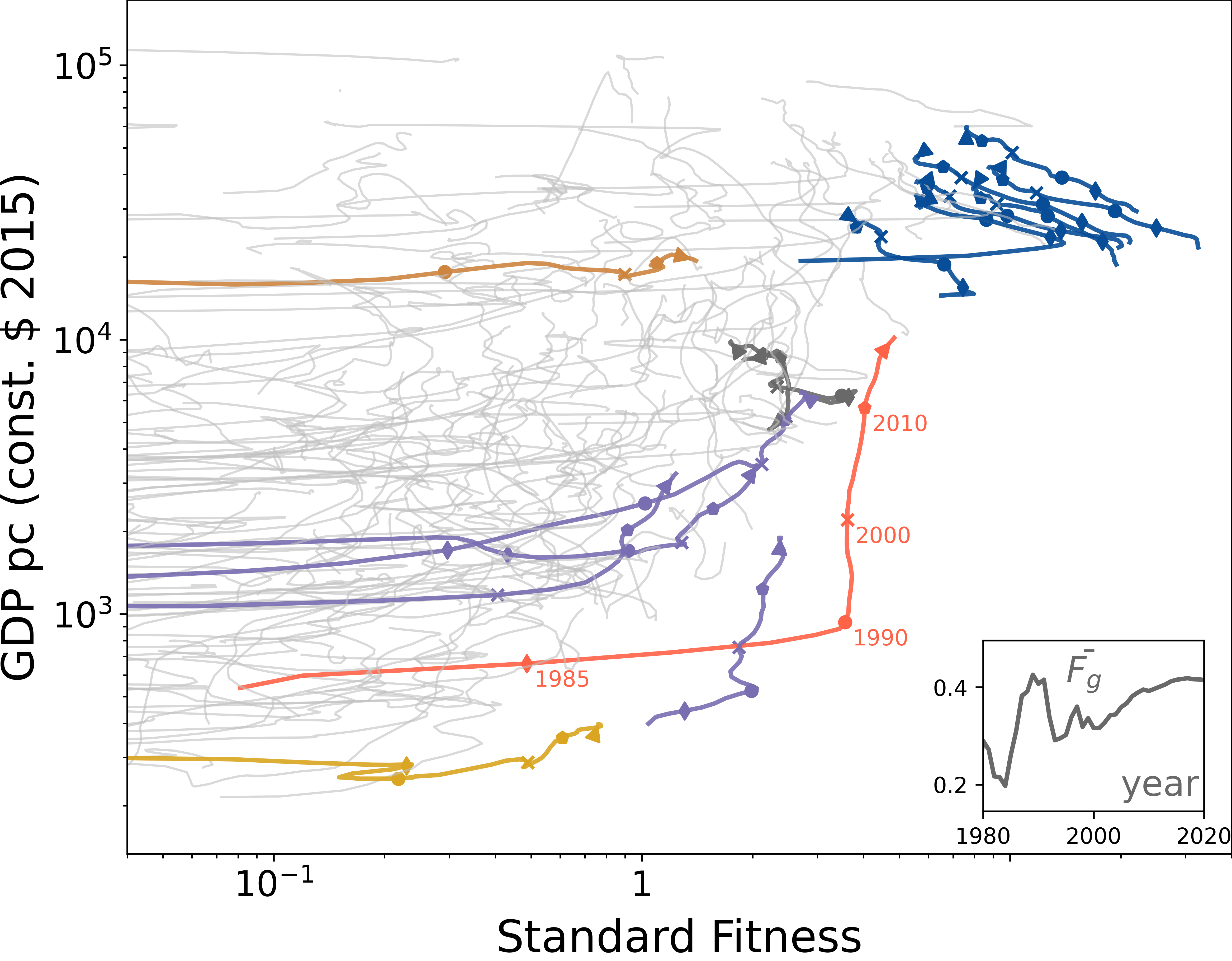
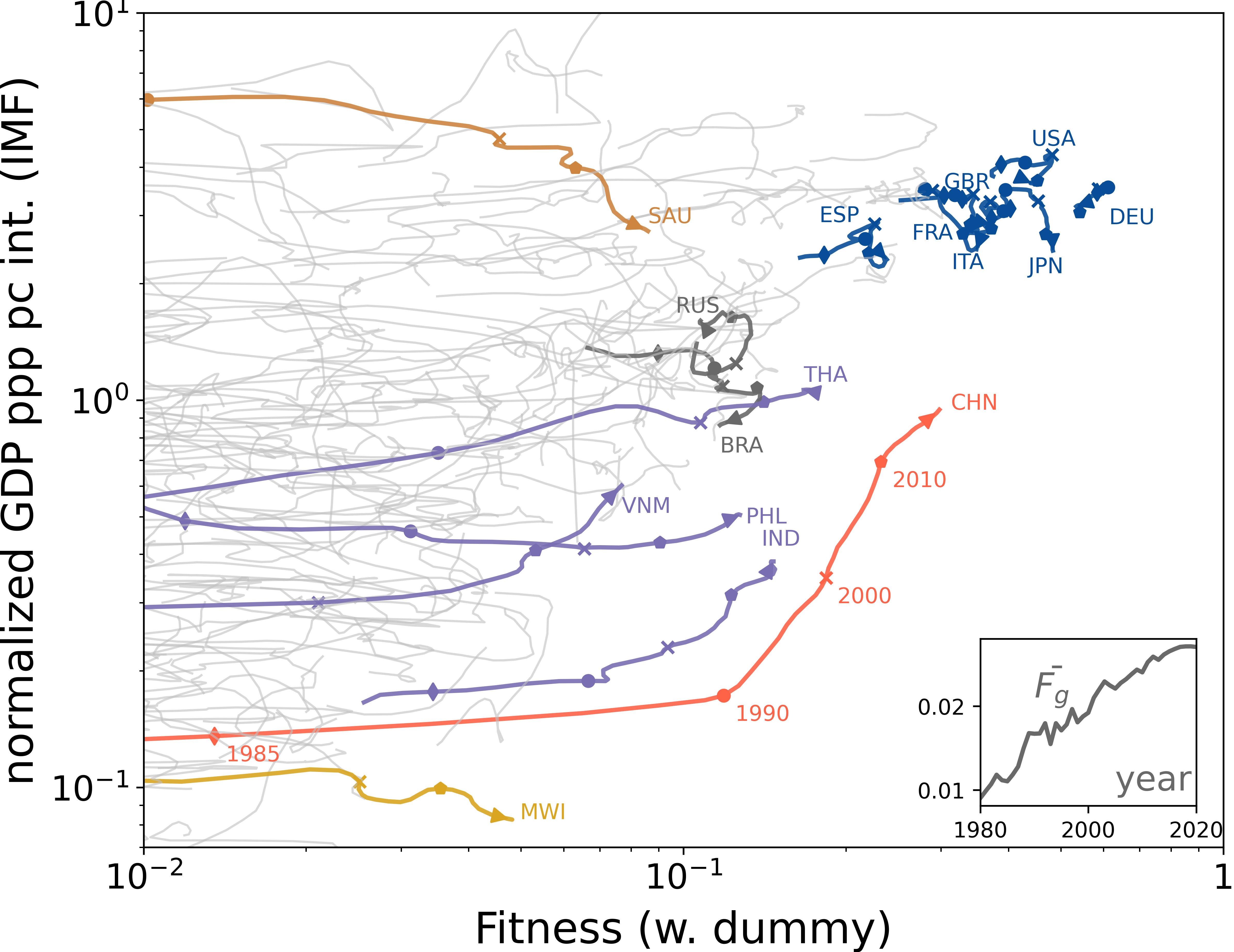
Function highlights that the natural scale of the fitness score is the logarithmic scale, as often considered in many diagrams (for example, the Income-Fitness diagram in [1]), because the problem corresponds to a constrained optimization problem with logarithmic constraint barrier. In fact, for relevant applications (see for example [3, 4]), a logarithmic transformation is required in order to have well-separated values of Fitness and Complexity, as for example in the visualization of countries’ trajectories in figure 2.
Potentials.
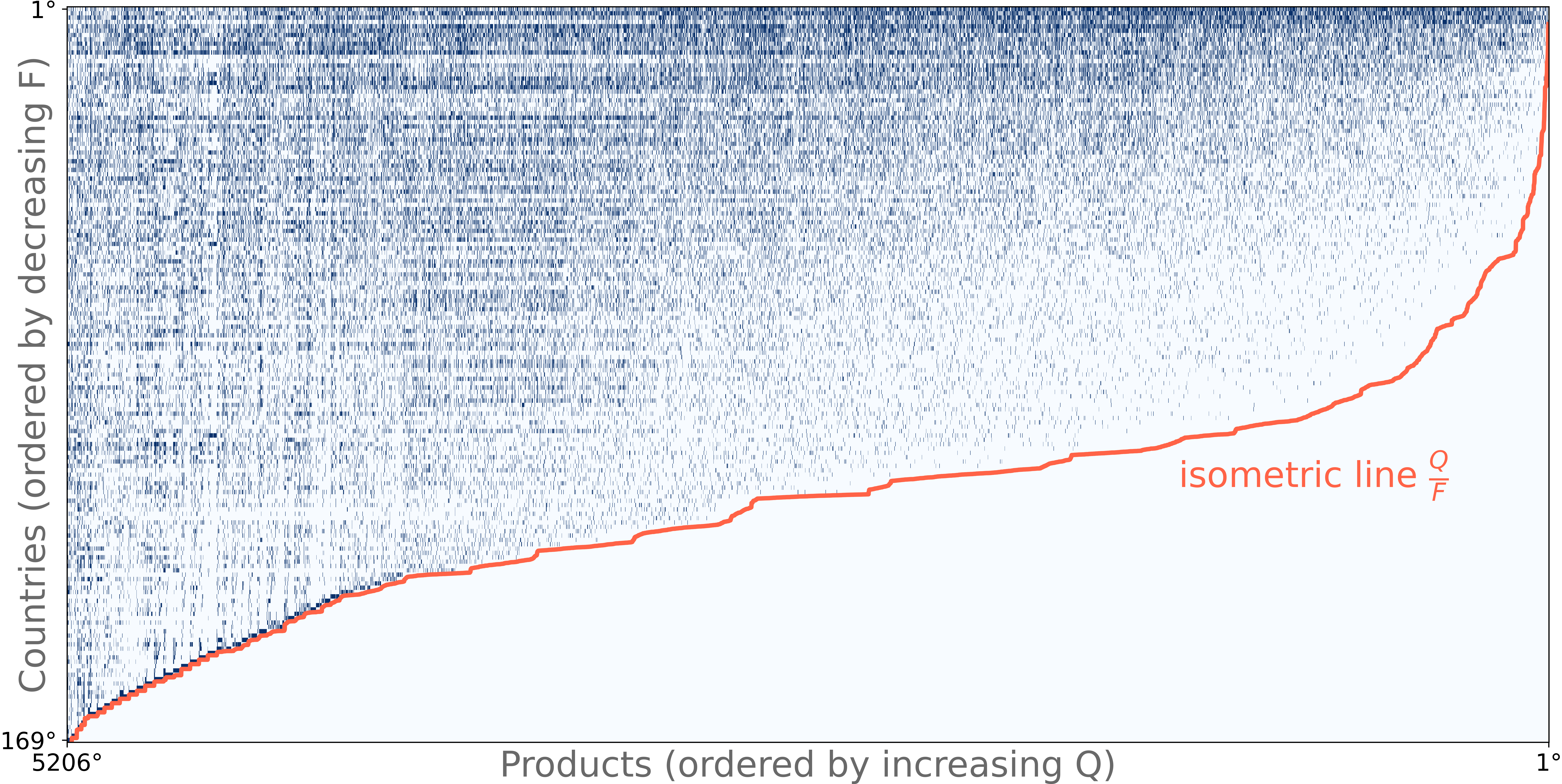
Further, a well known property of FC is its ability to reorder rows and columns of in order to obtain a upper-left triangular matrix which highlights its nestedness [25], as shown in figure 1.

This can be obtained by simply reordering rows and columns of the matrix by the ranking of and , and this feature can be explained in terms of potentials functions (also called Kantorovich potentials). The Fitness of a country measures its industrial system’s capability while the Complexity is a measure of how hard is to produce each commodity. Thus, the region of the matrix with high and low should not be populated, by construction, because that would mean low Fitness countries producing highly complex products. Indeed, the two logarithmic potentials in eq. 5 define a barrier that cannot be overcome: here is a value of whose constant-value line defines the separation between the feasible and forbidden regions of the matrix. Translated in terms of Fitness and Complexity, we can find a value of that defines a barrier line in the reordered shapes that meets the same requirements with striking precision, see fig. 1 where we plot the isometric line with the lowest value among all the lines that define a completely empty region under the curve. This explains why in many real systems, by rearranging the matrix’s rows and columns by FC, the parts of the rearranged matrix exhibit a continuous border line.
Taking further our interpretation, the sum corresponds to the constant vector , up to a scale (see below), as assumed in FC. Let us now interpret as the amount of energy associated with the production of by country . Under this interpretation, constraint represents the total energy possessed by country , and we assume fair availability of energy resources among nations. The fairness assumption is enforced by the condition that is homogeneous across countries, which makes the FC algorithm independent of country-level properties other than their export basket composition. Every country allocates resources into its productive system by distributing them among the production of different products; this information is encoded in . On the other hand, the ability of different countries to produce a product is not fairly-distributed: at different levels of complexity , the energy cost differs. This means that each given resource unit can be exploited with different efficiency by countries with different Fitness , and the energy cost change accordingly to the ratio of the two metrics. Therefore, the forbidden region of , displayed in fig. 1, is simply represented by too-expensive products in terms of resource allocation. heterogeneity of resources owned by countries can be naturally introduced in this framework in further studies, see conclusions.
Scale invariance.
Another feature that FC inherits from the logarithmic barrier function is that presents a symmetry and, as a consequence, the stationary solutions of equation 5 are not unique. The transformation with leaves invariant the value of , which allows a rescaling of the fixed points. At the level of the numerical implementations of the algorithm, the rescaling helps to increase the numerical precision and consequently the stability of the codes [18]. Instead, on the conceptual ground, the rescaling symmetry states that the fixed point solutions are not uniquely defined, rather a scale must be chosen to break the symmetry. The scale becomes particularly relevant when we are interested to compare the Fitness scores derived from different matrices, such as when comparing the Fitness scores of the same countries at two different years.
There are different ways to set a scale. For example, it is possible to select a single country or a product as a reference, as proposed by [26]. Another possibility to define a scale, which we introduce here, is to add a dummy country able to produce all the products, thus adding a full row of ones to the matrix. The value at the fixed point of the dummy country’s Fitness sets the scale by requiring that at any time its value is fixed to a constant (e.g. 1). Setting the scale provides a formal method to compare different matrices, and it affects only the Fitness scores and trajectories and not the ranking.


Using the International Trade export 222We use the COMTRADE data based on the SITC v2 classification started in 1976 because we are interested to a long term dynamics. If the objective was to obtain state-of-the-art predictions, the classification provided by the Harmonized System is preferable, as it is updated regularly., we verify that the trajectories in the Income - Fitness diagram can be substantially affected by the choice of the Fitness’ scale. Figure 2 shows in the right panel that when we fix the Fitness score of the dummy country, the Fitness of western countries (blue lines) does not evolve appreciably over more than 4 decades, whereas many Asian countries (purple lines), and China on top (red line), are catching up the wealth and developed nations. Instead when we the scale is fixed by the normalization condition as in the original paper [1], we observe that the Fitness of wealthy countries decreases in time, as shown in the left panel. Our finding suggest that this trend is a manifestation of the catching up phenomenon . The same effect can be observed in the Income variable, since removing the global income average, make stationary most of the wealth countries. The main takeaways from these results is that while ether scale-invariance of potential allows the researcher to set the scale, this choice should be made cautiously, as it affects the resulting fitness temporal trajectories and their interpretation.
Possible development pathways.
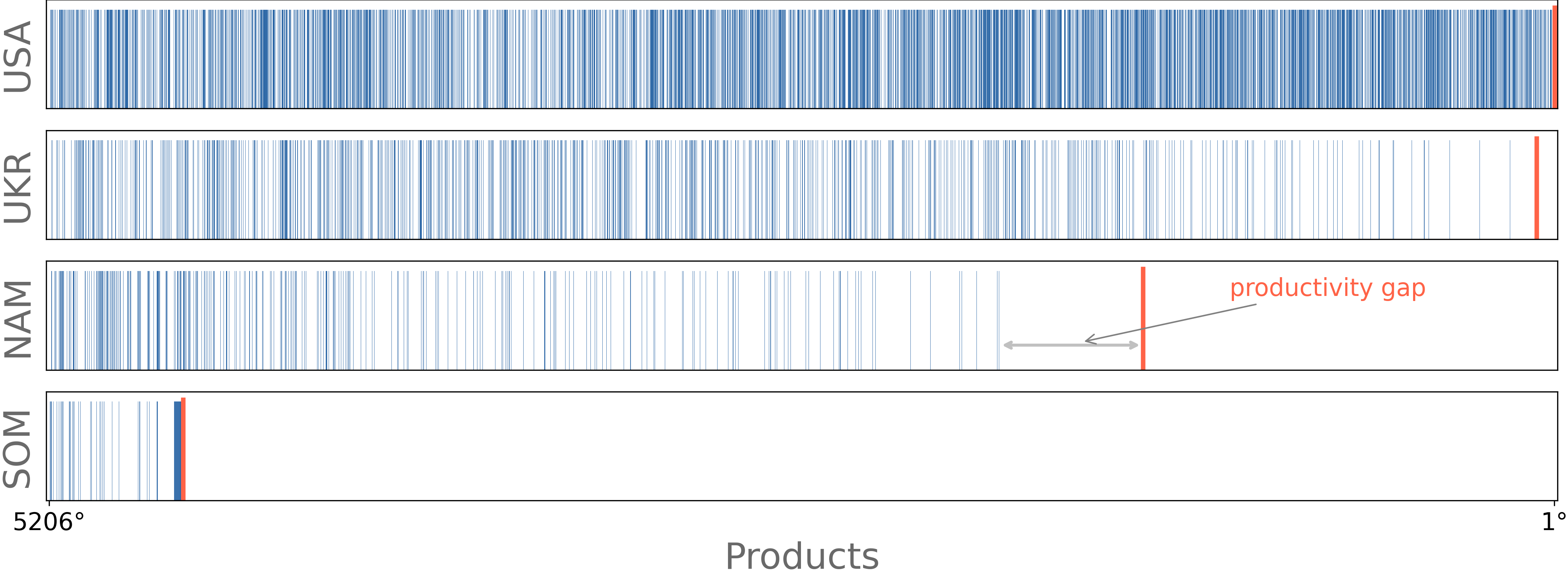
The existence of a potential barrier makes it also possible to identify Fitness as the maximum sophistication achievable by products exported from each country, which is represented by the isometric line of the matrix. However, most of the developed countries do not export products lying on the isometric line (see Fig. 1), and exhibit a lower density of exported products near the isometric line, which indicates a productivity gap with respect to the maximum product-Complexity level achievable from their Fitness. This pattern suggests that different nations might benefit from pursuing different strategies to increase their capabilities and ultimately their wealth. We conjecture below that different countries might benefit from three different classes of new product development strategies:
-
•
Learner pathway, which might be suited for low-Fitness countries that are at their maximum level of capabilities and already reached the isometric line. A clear example is Somalia in Fig. 3. These countries might benefit from enhancing their industrial system by increasing the relevant capabilities before entering new markets.
-
•
Exploiter pathway, which might be suited for medium-Fitness countries, such as Namibia and Ukraine, whose spectra of exported products [27] lie far from the isometric line or who exhibit low-density of exports near the line. These countries may have unexpressed capabilities, and could benefit from investing in the production of goods already allowed by their capabilities.
-
•
Explorer pathway, which might be suited for high-fitness countries that present a dense spectrum along the entire axis (see USA in the figure). These countries might be already efficiently exploiting their capabilities. Therefore, their best strategy might be to move from exploitation of existing capability to the exploration of new, and thus not classified, activities and goods.

Clearly, Fitness is a single parameter and cannot fully explain the productivity gaps. A finer description of export baskets is needed to identify opportunities for new products and optimal development strategies. For example, our simplified classification could be integrated with network-based approaches [28] and machine learning approaches [29] zto better predict product development probabilities, which might suggest new future development pathways for countries.
4 Conclusions
We showed the deep connection between the Fitness and Complexity algorithm, developed in Economic Complexity, and the Sinkhorn-Knopp algorithm devised in matrix scaling. Indeed, despite minor differences in the algorithms’ structure, the fixed points of the two algorithms coincide. This connection allowed us to better understand some properties of FC and interpret Fitness and Complexity as potentials of a suitable energy function of mutualistic systems such as the international trade web. This description indicates how countries deploy their units of resources, it allows the definition of a barrier that defines the inaccessible region of country-product matrix, and it helps us to classify countries by their exploited potential, which suggests different strategies of investment and development. Differences in resources can be accounted for in the next future by leveraging a key property of SK: SK can be used to solve the Optimal Transport problem [30]. Leveraging this property could pave the way to a vast mathematical and economic theory to be explored in future works.
Appendix A Stability of the fixed point
The stability of the fixed point can be evaluated better by focusing on the potentials, a.k.a. the logarithms of . The logarithmic barrier function reads
| (6) |
where the matrix and the constraint depend on the previous terms through
| (7) |
The Hessian at the fixed point ( s.t. ) can be written as
| (8) |
The Hessian matrix is a symmetric diagonally dominant matrix with real non-negative diagonal entries, hence it is positive semidefinite [31]. Therefore, the fixed-point solution is marginally stable, since we already know and discuss in the main text that there is at least one direction of constant energy related to the scale invariance symmetry.
References
References
- [1] Andrea Tacchella, Matthieu Cristelli, Guido Caldarelli, Andrea Gabrielli, and Luciano Pietronero. A New Metrics for Countries’ Fitness and Products’ Complexity. Scientific Reports, 2:1–7, 2012.
- [2] Matthieu Cristelli, Andrea Gabrielli, Andrea Tacchella, Guido Caldarelli, and Luciano Pietronero. Measuring the Intangibles: A Metrics for the Economic Complexity of Countries and Products. PLoS ONE, 8(8), 2013.
- [3] Justin Lin, Masud Cader, and Luciano Pietronero. What african industrial development can learn from east asian successes: The role of complexity and economic fitness. Emcompass notes 88, International Finance Corporation, World Bank, 2020.
- [4] Pugliese E and Tacchella A. Economic complexity analytics: Country factsheets. (KJ-NA-30711-EN-N (online)), 2021.
- [5] Andrea Tacchella, Dario Mazzilli, and Luciano Pietronero. A dynamical systems approach to gross domestic product forecasting. Nature Physics, 14(8):861–865, aug 2018.
- [6] Manuel Sebastian Mariani, Alexandre Vidmer, Matsúš Medo, and Yi-Cheng Zhang. Measuring economic complexity of countries and products: which metric to use? The European Physical Journal B, 88(11):1–9, 2015.
- [7] Rui-Jie Wu, Gui-Yuan Shi, Yi-Cheng Zhang, and Manuel Sebastian Mariani. The mathematics of non-linear metrics for nested networks. Physica A: Statistical Mechanics and its Applications, 460:254–269, 2016.
- [8] Vito D. P. Servedio, Paolo Buttà , Dario Mazzilli, Andrea Tacchella, and Luciano Pietronero. A new and stable estimation method of country economic fitness and product complexity. Entropy, 20(10), 2018.
- [9] Virginia Domínguez-García and Miguel A Munoz. Ranking species in mutualistic networks. Scientific reports, 5(1):1–7, 2015.
- [10] Jian-Hong Lin, Claudio Juan Tessone, and Manuel Sebastian Mariani. Nestedness maximization in complex networks through the fitness-complexity algorithm. Entropy, 20(10):768, 2018.
- [11] Andrea Zaccaria, Michela Del Vicario, Walter Quattrociocchi, Antonio Scala, and Luciano Pietronero. Poprank: Ranking pages’ impact and users’ engagement on Facebook. PLoS ONE, 14(1):6–8, 2019.
- [12] Richard Dennis Sinkhorn and Paul Joseph Knopp. Concerning nonnegative matrices and doubly stochastic matrices. Pacific Journal of Mathematics, 21(2):343–348, 1967.
- [13] Gabriel Peyré and Marco Cuturi. Computational optimal transport. Foundations and Trends in Machine Learning, 11(5-6):1–257, 2019.
- [14] Richard A. Brualdi. Combinatorial Matrix Classes. Cambridge University Press, Cambridge, 2006.
- [15] Martin Idel. A review of matrix scaling and sinkhorn’s normal form for matrices and positive maps, 2016.
- [16] Flaviano Morone. Clustering matrices through optimal permutations. Journal of Physics: Complexity, 3(3):035007, 2022.
- [17] Emanuele Pugliese, Andrea Zaccaria, and Luciano Pietronero. On the convergence of the Fitness-Complexity algorithm. The European Physical Journal Special Topics, 225(10):1893–1911, 2016.
- [18] Alexis Thibault, Lénaic Chizat, Charles Dossal, and Nicolas Papadakis. Overrelaxed sinkhorn-knopp algorithm for regularized optimal transport. Algorithms, 14(5), 2021.
- [19] Philip A. Knight. The sinkhorn-knopp algorithm: Convergence and applications. SIAM J. Matrix Anal. Appl., 30(1):261–275, mar 2008.
- [20] Richard A Brualdi. Matrices of 0’s and 1’s with total support. Journal of Combinatorial Theory, Series A, 28(3):249–256, 1980.
- [21] Robert J. Berman. The sinkhorn algorithm, parabolic optimal transport and geometric monge-ampère equations. Numerische Mathematik, 145(4):771–836, 2020.
- [22] Kristen Anderson, Ashley Burt, Will Cousins, Brent Hancock, and David Strong. A Sinkhorn-Knopp Fixed Point Problem *. pages 1–11, 2010.
- [23] Albert W Marshall and Ingram Olkin. Scaling of matrices to achieve specified row and column sums. Numerische Mathematik, 12(1):83–90, 1968.
- [24] C. A. Hidalgo and R. Hausmann. The building blocks of economic complexity. PNAS, 106, 2009.
- [25] Manuel Sebastian Mariani, Zhuo Ming Ren, Jordi Bascompte, and Claudio Juan Tessone. Nestedness in complex networks: Observation, emergence, and implications. Physics Reports, 813:1–90, 2019.
- [26] Aurelio Patelli, Lorenzo Napolitano, Giulio Cimini, and Andrea Gabrielli. Geography of science: Competitiveness and inequality, 2021.
- [27] Felipe G Operti, Emanuele Pugliese, José S Andrade Jr, Luciano Pietronero, and Andrea Gabrielli. Dynamics in the fitness-income plane: Brazilian states vs world countries. PloS one, 13(6):e0197616, 2018.
- [28] E. Pugliese, G. Cimini, A. Patelli, A. Zaccaria, L. Pietronero, and A. Gabrielli. Unfolding the innovation system for the development of countries: co-evolution of science, technology and production. Scientific Reports, 9, 2017.
- [29] Andrea Tacchella, Andrea Zaccaria, Marco Miccheli, and Luciano Pietronero. Relatedness in the era of machine learning, 2021.
- [30] Marco Cuturi. Sinkhorn distances: Lightspeed computation of optimal transport. Advances in Neural Information Processing Systems, pages 1–9, 2013.
- [31] Roger A. Horn and Charles R. Johnson. Matrix Analysis. Cambridge University Press, 2 edition, 2012.