Spin vectors in the Koronis family: IV. Completing the sample of its largest members after 35 years of study

Abstract

An observational study of Koronis family members’ spin properties was undertaken with two primary objectives: to reduce selection biases for object rotation period and lightcurve amplitude in the sample of members’ known spin vectors, and to better constrain future modeling of spin properties evolution. Here we report rotation lightcurves of nineteen Koronis family members, and derived results that increase the sample of determined spin vectors in the Koronis family to include 34 of the largest 36 family members, completing it to $H\approx 11.3$ ($D\sim 16$ km) for the largest 32 members. The program observations were made during a total of 72 apparitions between 2005–2021, and are reported here along with several earlier unpublished lightcurves. All of the reported data were analyzed together with previously published lightcurves to determine the objects’ sidereal rotation periods, spin vector orientations, and convex model shape solutions. The derived distributions of retrograde rotation rates and pole obliquities appear to be qualitatively consistent with outcomes of modification by thermal YORP torques. The distribution of spin rates for the prograde rotators remains narrower than that for the retrograde rotators; in particular, the absence of prograde rotators having periods longer than about 20 h is real, while among the retrograde rotators are several objects having longer periods up to about 65 h. None of the prograde objects newly added to the sample appear to be trapped in an $s_{6}$ spin-orbit resonance that is characteristic of most of the largest prograde objects (Vokrouhlický et al., 2003); these smaller objects either could have been trapped previously and have already evolved out, or have experienced spin evolution tracks that did not include the resonance.

Koronis family spin vector sample completed to largest 32 members ($\sim 16$ km diameter)

Removal of sample selection biases for interpreting and modeling spin evolution

The absence of prograde spins having rotation periods longer than about 20 h is real

Smaller prograde objects avoided or escaped the spin-orbit trapping of larger objects

Epochs analysis combined with convex inversion is effective to determine spin vectors

1 Introduction

Studies of spin vector orientations among members of asteroid families provide valuable information to constrain models of asteroid spin evolution processes. Members of a family comprise a group of asteroids that were formed together from the outcome of collisional disruption of a parent body, sharing the same physical structure as reaccumulated gravitational aggregates, the same age since formation, and similar evolution for similar lengths of time. Thus family members serve as a constrained sample that avoids difficulties of interpreting a distribution of spin properties which does not share a common origin and dynamical history.

Prior to determinations of thirteen Koronis family members’ spin vectors by SLIV03; SLIV09, spin vectors of main belt asteroids smaller than about 40 km had not been much explored, nor had there been a systematic program of spin vector determinations within any particular asteroid family, although statistically larger lightcurve amplitudes of Koronis family asteroids gave an early indication that Koronis family spin vectors might have some preferential alignment (BINZ88; BINZ90). The markedly non-random distribution of measured spin vectors determined initially from observations of ten of the largest Koronis family members (SLIV02) revealed evidence of modification of their spins by YORP thermal radiation torques, in some cases combined with solar and planetary gravitational torques (VOKR03). The distribution of spin vectors among the previously studied sample is dominated by two groupings: a group of low-obliquity retrograde spins spanning a wide range of periods between about 3 h and 30 h, and a smaller group of prograde spins with obliquities near 45${}^{\circ}$ and periods near 8 h, characteristic of trapping in the $s_{6}$ spin-orbit resonance (VOKR03). A single “stray” longer-period, low-obliquity prograde object (SLIV09) subsequently was joined by the largest family member (208) Lacrimosa (VOKR21) which initially had been misidentified as being in the retrograde group based on an alias sidereal period.

A limitation of the previously studied Koronis family spin vector sample comprising 13 of the largest 18 family members, as classified by MOTH05 and using relative catalog absolute magnitudes $\mathit{H}$ from the coincident compilation by THOL09 as a proxy for relative sizes, is that selection biases render that sample complete to only the largest 8 members. Although that set of spin vectors was sufficient to have revealed evidence of YORP modification in the distribution of spin rates and spin obliquities, the small size of the completed sample and the presence of bias effects limit its usefulness for further understanding of the spin evolution. In particular, because the rate at which YORP acts on a body is size-dependent, one may expect systematic study of smaller members of the family to reveal information that is not apparent from the distribution of spin vectors in the incomplete sample of larger members.

KRYS07 noted the need for more spin vector data for family main belt asteroids; subsequently KRYS13 studied spin vectors of 18 members of the Flora family and reported evidence of YORP modification, identifying at least three objects which may be trapped in a so-called “Slivan state” spin-orbit resonance as described by VOKR03. KIM14 studied spin vectors of 13 members of the Maria family and did not detect spin vector alignment, but did find evidence of YORP modification of spin rates in a sample of 92 members. HANU13b investigated anisotropy of spin vectors in eight asteroid families including Koronis, Flora, and Maria, corroborating finding depopulation of poles close to the ecliptic plane, but did not find any candidates for spin-orbit resonance trapping in their 38-member sample from the Flora family. In each of the studies the families’ spin vector samples were not controlled for completeness to any particular size.

Obtaining the data needed for a deliberate spin vector determination program represents a considerable observing effort necessarily spanning a number of years. Determination of a spin vector from ground-based lightcurve observations requires that the data set (a) includes observations from a sufficient number of different viewing aspects, (b) spans an interval of time long enough to precisely determine the object’s sidereal rotation period, and (c) samples a sufficient progression of shorter time intervals within the long time span to rule out alias sidereal periods. Given that the viewing geometry of a Koronis family member changes very little during any particular apparition, observations from at least five to six apparitions are needed to assemble a suitable lightcurve data set. SLIV08a have described a long-term observing program designed and undertaken specifically to obtain the rotation lightcurve data needed to increase the sample of determined Koronis family spin vectors; most of the lightcurves newly reported in the present work were obtained as part of that program.

The new lightcurves, like those used to determine the previously-studied sample of Koronis family spin vectors, would now be characterized as densely-sampled in time in contrast with sparsely-sampled lightcurve data from sky imaging surveys. Several years into the multi-year observing program, DURE09 independently described a method to exploit the increasing availability of sparse-in-time lightcurves by combining them with a smaller number of densely-sampled lightcurves, provided that the sparse data brightnesses have been calibrated to some common zero-point so that they can be assembled into lightcurves. The availability and quality of sparse data to construct a specific sample of any particular asteroids of interest remain subject to the observing parameters of the sky surveys, including cadence and targeted brightness range. Applications of this “sparse data” approach (HANU11; HANU13b; DURE16; DURE18a; DURE18b; DURE19; DURE20) have yielded spin vector determinations for fifteen of the observing program objects; a comparison of those results with spin vectors determined in the present work for the same objects, using the same underlying convex modeling approach and assumptions, but based instead on independent sets of densely-sampled input lightcurves, is included in Sec. LABEL:DISC-SEC.

In this paper the lightcurve observations and analyses for spins and convex shape models of nineteen Koronis family members are reported, completing the sample of determined spin vectors in the Koronis family down to $H\approx 11.3$ ($D\sim 16$ km). The results reduce selection biases in the set of known spin vectors for family members, and will constrain future modeling of spin properties evolution; in the meantime, the spin properties in the expanded sample are briefly discussed.

Catalog physical properties for the observing program objects are summarized in Table 1, which lists for each object its catalog absolute magnitude $\mathit{H}$, available taxonomic classifications, and whether a spectrum has been reported. Taxonomic types have been determined for seventeen of the objects, all of which are classified as either some variety of S-type, or for (1100) Arnica as a union set of two types that includes S-type.

Table 1: Catalog physical properties for the observing program objects.

Asteroid	Catalog $\mathit{H}$	Taxonomic	Spectrum	Taxonomy
	(notes a,b)	classification(s)	reported?	reference
(658) Asteria	10.51	S	–	NEES10
(761) Brendelia	10.74	S, SC	–	NEES10; HASS12
(811) Nauheima	10.77	S, S0, LS	–	NEES10; HASS12
(975) Perseverantia	10.50	S	–	NEES10
(1029) La Plata	10.92	S	–	NEES10; HASS12
(1079) Mimosa	11.19	S	–	NEES10; HASS12
(1100) Arnica	10.94	LS	–	HASS12
(1245) Calvinia	9.98	S, S0	–	NEES10
(1336) Zeelandia	10.67	S, S0	yes	NEES10
(1350) Rosselia	10.73	S, Sa	yes	NEES10
(1423) Jose	10.97	S	yes	NEES10; HASS12
(1482) Sebastiana	11.10	–	–
(1618) Dawn	11.23	S	yes	NEES10
(1635) Bohrmann	11.08	S	yes	NEES10
(1725) CrAO	11.37	S	yes	NEES10
(1742) Schaifers	11.32	S	–	HASS12
(1848) Delvaux	11.11	S	yes	NEES10
(2144) Marietta	11.35	S	–	HASS12
(2209) Tianjin	11.26	–	–

${}^{\rm a}$ Catalog $\mathit{H}$ values published in various Minor Planets and Comets Orbit Supplements from the IAU Minor Planet Center, and curated by the Solar System Dynamics group at the NASA Jet Propulsion Laboratory. Retrieved using the JPL Small-Body Database Lookup Web tool https://ssd.jpl.nasa.gov/tools/sbdb_lookup.html on 2022 March 28.
${}^{\rm b}$ Use of catalog $\mathit{H}$ in the present work is limited to serving as proxy for approximate relative sizes of the family members. Solar phase parameters derived from observing program data are reported in Table 6.

2 Observations

The observing program used CCD imaging cameras at nine different observatories from 2005 September through 2021 August, recording 443 individual rotation lightcurves of the nineteen target objects during 72 different apparitions. Once observations of a target were begun during an apparition, particular efforts were made to obtain complete coverage in rotation phase at a sampling rate of at least 50 points per rotation in order to maximize usefulness of the data for spin vector analyses, and obtaining data to also determine a more precise rotation period was prioritized for objects whose existing period determination was not precise enough to meet the criterion described by SLIV12b. During most apparitions, observations were made to calibrate the lightcurves to standard magnitudes by observing solar-colored standard stars from LAND83; LAND92, and when possible, additional observations were made to increase solar phase angle coverage. Images were processed and measured using standard techniques for synthetic aperture photometry. Also reported here with the observing program data are several previously unpublished lightcurves from one earlier apparition.

Observing circumstances for each object are presented in Table 2, summarized by apparition. The table lists for each apparition the UT date month(s) during which the observations were made, the number of individual lightcurves observed, the approximate ecliptic longitude $\lambda_{\rm PAB}$ and latitude $\beta_{\rm PAB}$ (J2000) of the phase angle bisector, the range of solar phase angles $\alpha$ observed, and the filter(s) and telescope used. Information about the telescopes, observatories, and detectors is presented in Table 3. Rotation period results are presented in Table 4, which lists for each object the observed range of peak-to-peak lightcurve amplitudes and the derived periods with their uncertainties. For periods improved during this study the apparition whose lightcurves yield the most precise result is identified. Color index results are summarized in Table 5.

Table 2: Summarized observing circumstances.

Object	UT date(s)	$N_{\rm lc}$	$\lambda_{\rm PAB}$	$\beta_{\rm PAB}$	$\alpha$	Filter(s)${}^{\rm a}$	Telescope
(658) Asteria	2007 Sep	4	340${}^{\circ}$	0${}^{\circ}$	0${}^{\circ}$–4${}^{\circ}$	$\mathit{V}$	b
(761) Brendelia	2005 Sep–Nov	21	353${}^{\circ}$	$-$1${}^{\circ}$	2${}^{\circ}$–18${}^{\circ}$	$\mathit{V,R}$	b
	2006 Dec–2007 Feb	21	90${}^{\circ}$	+2${}^{\circ}$	2${}^{\circ}$–16${}^{\circ}$	$\mathit{V}$	b
	2008 Jan–Apr	19	170${}^{\circ}$	+1${}^{\circ}$	1${}^{\circ}$–16${}^{\circ}$	$\mathit{V,R}$	b
	2009 May–Jun	9	260${}^{\circ}$	$-$2${}^{\circ}$	3${}^{\circ}$–9${}^{\circ}$	$\mathit{V}$	b,c
	2013 Mar–May	14	183${}^{\circ}$	+1${}^{\circ}$	3${}^{\circ}$–17${}^{\circ}$	$\mathit{R}$	b
(811) Nauheima	2005 Dec–2006 Feb	3	98${}^{\circ}$	$-$2${}^{\circ}$	5${}^{\circ}$–17${}^{\circ}$	$\mathit{V}$	b
	2007 Feb–Mar	2	174${}^{\circ}$	+3${}^{\circ}$	3${}^{\circ}$–7${}^{\circ}$	$\mathit{V}$	b
(975) Perseverantia	2005 Sep	1	357${}^{\circ}$	$-$2${}^{\circ}$	6${}^{\circ}$	$\mathit{V}$	b
	2006 Nov–2007 Feb	6	97${}^{\circ}$	+3${}^{\circ}$	6${}^{\circ}$–19${}^{\circ}$	$\mathit{V,R}$	b
	2008 Mar–Apr	4	197${}^{\circ}$	+1${}^{\circ}$	3${}^{\circ}$–9${}^{\circ}$	$\mathit{V}$	b
	2013 May	5	218${}^{\circ}$	0${}^{\circ}$	2${}^{\circ}$–6${}^{\circ}$	$\mathit{R}$	b
(1029) La Plata	2005 Dec	4	78${}^{\circ}$	+2${}^{\circ}$	1${}^{\circ}$–3${}^{\circ}$	$\mathit{V}$	b
	2007 Mar–Apr	4	173${}^{\circ}$	+2${}^{\circ}$	1${}^{\circ}$–15${}^{\circ}$	$\mathit{V}$	b
(1079) Mimosa	1984 Nov	5	68${}^{\circ}$	+2${}^{\circ}$	1${}^{\circ}$–4${}^{\circ}$	$\mathit{B}$	k
	2013 Oct–Nov	14	43${}^{\circ}$	+1${}^{\circ}$	1${}^{\circ}$–13${}^{\circ}$	$\mathit{R}$	b
	2016 Apr–May	8	235${}^{\circ}$	$-$1${}^{\circ}$	1${}^{\circ}$–7${}^{\circ}$	$\mathit{R}$	l
	2017 Jul–Aug	11	319${}^{\circ}$	0${}^{\circ}$	2${}^{\circ}$–8${}^{\circ}$	$\mathit{R}$	l
	2021 May–Jul	30	247${}^{\circ}$	$-$1${}^{\circ}$	6${}^{\circ}$–18${}^{\circ}$	$\mathit{r^{\prime},R}$	m,n
(1100) Arnica	2007 Sep–Nov	7	20${}^{\circ}$	+1${}^{\circ}$	1${}^{\circ}$–12${}^{\circ}$	$\mathit{V,R}$	b
	2009 Jan–Mar	9	111${}^{\circ}$	0${}^{\circ}$	3${}^{\circ}$–18${}^{\circ}$	$\mathit{V,R}$	b
	2010 Feb–Apr	7	188${}^{\circ}$	$-$1${}^{\circ}$	2${}^{\circ}$–12${}^{\circ}$	c	d
	2011 May–Jun	6	279${}^{\circ}$	$-$1${}^{\circ}$	3${}^{\circ}$–14${}^{\circ}$	$\mathit{V}$	c,e
	2012 Sep–2013 Jan	6	32${}^{\circ}$	+1${}^{\circ}$	1${}^{\circ}$–20${}^{\circ}$	$\mathit{V,R}$	b
	2014 Jan	5	115${}^{\circ}$	0${}^{\circ}$	2${}^{\circ}$–6${}^{\circ}$	$\mathit{R}$	b
(1245) Calvinia	2006 Jul	3	269${}^{\circ}$	+3${}^{\circ}$	9${}^{\circ}$–13${}^{\circ}$	$\mathit{V}$	b
	2007 Oct	1	15${}^{\circ}$	$-$3${}^{\circ}$	4${}^{\circ}$	$\mathit{V}$	b
	2012 Dec	1	26${}^{\circ}$	$-$3${}^{\circ}$	17${}^{\circ}$	$\mathit{V}$	b
(1336) Zeelandia	2006 Oct	5	335${}^{\circ}$	$-$4${}^{\circ}$	14${}^{\circ}$–20${}^{\circ}$	$\mathit{V,R}$	b
	2007 Nov-Dec	2	72${}^{\circ}$	$-$2${}^{\circ}$	2${}^{\circ}$	$\mathit{V}$	b
	2009 Mar–Apr	3	155${}^{\circ}$	+3${}^{\circ}$	7${}^{\circ}$–17${}^{\circ}$	$\mathit{V,R}$	b
	2010 Jun	5	245${}^{\circ}$	+2${}^{\circ}$	4${}^{\circ}$–7${}^{\circ}$	$\mathit{V}$	c
	2011 Aug–Oct	6	352${}^{\circ}$	$-$4${}^{\circ}$	8${}^{\circ}$–14${}^{\circ}$	$\mathit{V}$	e
	2013 Jan–Mar	4	91${}^{\circ}$	0${}^{\circ}$	8${}^{\circ}$–19${}^{\circ}$	$\mathit{R}$	b
	2014 Mar–Apr	6	170${}^{\circ}$	+4${}^{\circ}$	7${}^{\circ}$–14${}^{\circ}$	$\mathit{R}$	b
(1350) Rosselia	2006 Sep	3	335${}^{\circ}$	$-$1${}^{\circ}$	6${}^{\circ}$–10${}^{\circ}$	$\mathit{V,R}$	b
	2007 Dec	2	89${}^{\circ}$	$-$3${}^{\circ}$	1${}^{\circ}$–2${}^{\circ}$	$\mathit{V}$	b
(1423) Jose	2006 Jan–Mar	6	139${}^{\circ}$	+4${}^{\circ}$	4${}^{\circ}$–14${}^{\circ}$	$\mathit{V}$	b
	2007 Apr–Jun	7	218${}^{\circ}$	+1${}^{\circ}$	2${}^{\circ}$–14${}^{\circ}$	$\mathit{V}$	b,f
(1482) Sebastiana	2006 Mar–Apr	4	151${}^{\circ}$	+$4^{\circ}$	5${}^{\circ}$–18${}^{\circ}$	$\mathit{V}$	b
	2007 May–Jun	4	244${}^{\circ}$	$0^{\circ}$	1${}^{\circ}$–9${}^{\circ}$	$\mathit{V}$	b
(1618) Dawn	2014 Jan	5	99${}^{\circ}$	0${}^{\circ}$	3${}^{\circ}$–12${}^{\circ}$	$\mathit{R}$	b
	2015 Feb–Apr	11	187${}^{\circ}$	+4${}^{\circ}$	2${}^{\circ}$–15${}^{\circ}$	$\mathit{R}$	b
	2017 Oct–Dec	9	25${}^{\circ}$	$-$4${}^{\circ}$	2${}^{\circ}$–18${}^{\circ}$	$\mathit{R}$	b
	2020 Jun	4	205${}^{\circ}$	+3${}^{\circ}$	20${}^{\circ}$	$\mathit{R}$	i
	2021 Jun–Aug	12	299${}^{\circ}$	$-$1${}^{\circ}$	3${}^{\circ}$–15${}^{\circ}$	$\mathit{R}$	m

Table 2 (continued) Object UT date(s) $N_{\rm lc}$ $\lambda_{\rm PAB}$ $\beta_{\rm PAB}$ $\alpha$ Filter(s)${}^{\rm a}$ Telescope (1635) Bohrmann 2007 Jul–Aug 6 273${}^{\circ}$ +2${}^{\circ}$ 11${}^{\circ}$–18${}^{\circ}$ $\mathit{R}$ b 2008 Oct–Nov 10 20${}^{\circ}$ $-$1${}^{\circ}$ 1${}^{\circ}$–14${}^{\circ}$ $\mathit{V,R}$ b 2009 Nov–2010 Feb 6 110${}^{\circ}$ $-$2${}^{\circ}$ 3${}^{\circ}$–15${}^{\circ}$ $\mathit{V,R}$ b,d,g 2011 Apr–May 3 192${}^{\circ}$ +1${}^{\circ}$ 8${}^{\circ}$–11${}^{\circ}$ c d 2012 Jun–Jul 6 290${}^{\circ}$ +2${}^{\circ}$ 1${}^{\circ}$–11${}^{\circ}$ $\mathit{V,R}$ b,c (1725) CrAO 2014 Sep–Oct 8 353${}^{\circ}$ $-$3${}^{\circ}$ 3${}^{\circ}$–16${}^{\circ}$ $\mathit{V,r^{\prime}}$ b 2016 Jan–Feb 5 95${}^{\circ}$ $-$1${}^{\circ}$ 7${}^{\circ}$–15${}^{\circ}$ $\mathit{V,R}$ b 2017 Mar–Apr 7 171${}^{\circ}$ +3${}^{\circ}$ 4${}^{\circ}$–15${}^{\circ}$ $\mathit{R}$ b 2018 Jul–Aug 5 253${}^{\circ}$ +2${}^{\circ}$ 16${}^{\circ}$–20${}^{\circ}$ $\mathit{R}$ h 2019 Aug 3 356${}^{\circ}$ $-$3${}^{\circ}$ 10${}^{\circ}$–13${}^{\circ}$ $\mathit{R}$ h (1742) Schaifers 2007 Jul–Aug 6 289${}^{\circ}$ +2${}^{\circ}$ 2${}^{\circ}$–9${}^{\circ}$ $\mathit{R}$ b 2013 Oct–2014 Feb 12 51${}^{\circ}$ $-$3${}^{\circ}$ 2${}^{\circ}$–21${}^{\circ}$ $\mathit{V,R}$ b 2015 Feb 2 142${}^{\circ}$ $-$1${}^{\circ}$ 1${}^{\circ}$–4${}^{\circ}$ $\mathit{R}$ b 2016 Apr–May 2 217${}^{\circ}$ +3${}^{\circ}$ 1${}^{\circ}$–5${}^{\circ}$ $\mathit{R}$ b (1848) Delvaux 2006 Nov–Dec 2 336${}^{\circ}$ 0${}^{\circ}$ 20${}^{\circ}$ $\mathit{R}$ b 2009 Mar–Apr 2 152${}^{\circ}$ 0${}^{\circ}$ 10${}^{\circ}$–14${}^{\circ}$ $\mathit{V,R}$ b 2013 Feb 1 79${}^{\circ}$ +2${}^{\circ}$ 18${}^{\circ}$ $\mathit{R}$ b 2014 Apr 2 164${}^{\circ}$ $-$1${}^{\circ}$ 15${}^{\circ}$–17${}^{\circ}$ $\mathit{R}$ b 2015 Jun 1 259${}^{\circ}$ $-$2${}^{\circ}$ 6${}^{\circ}$ $\mathit{R}$ j (2144) Marietta 2007 Oct–Nov 4 28${}^{\circ}$ $-$3${}^{\circ}$ 2${}^{\circ}$–9${}^{\circ}$ $\mathit{V}$ b 2015 Mar–Jun 3 230${}^{\circ}$ +4${}^{\circ}$ 10${}^{\circ}$–15${}^{\circ}$ $\mathit{R}$ b 2016 Aug 1 313${}^{\circ}$ 0${}^{\circ}$ 1${}^{\circ}$ $\mathit{R}$ b (2209) Tianjin 2007 Nov–Dec 4 57${}^{\circ}$ $-$3${}^{\circ}$ 4${}^{\circ}$–10${}^{\circ}$ $\mathit{V}$ b 2009 Apr 6 162${}^{\circ}$ +1${}^{\circ}$ 15${}^{\circ}$–18${}^{\circ}$ $\mathit{V,R}$ b 2013 Feb–Apr 5 89${}^{\circ}$ $-$2${}^{\circ}$ 20${}^{\circ}$–21${}^{\circ}$ $\mathit{R}$ b 2014 Mar–Apr 6 178${}^{\circ}$ +2${}^{\circ}$ 4${}^{\circ}$–12${}^{\circ}$ $\mathit{R}$ b 2016 Sep 2 351${}^{\circ}$ $-$1${}^{\circ}$ 4${}^{\circ}$–5${}^{\circ}$ $\mathit{R}$ b

${}^{\rm a}$ Filters: $\mathit{B}$, Johnson $\mathit{B}$; $\mathit{V}$, Johnson $\mathit{V}$; $\mathit{R}$, Cousins $\mathit{R}$; $\mathit{r^{\prime}}$, SDSS $\mathit{r^{\prime}}$; c, colorless.
${}^{\rm b}$ 0.6-m Sawyer, Whitin Obs., observers S. Slivan and Corps of Loyal Observers, Wellesley Division (CLOWD)
${}^{\rm c}$ 0.4-m PROMPT, CTIO, observers S. Slivan, and in 2009 M. Hosek
${}^{\rm d}$ 0.35-m, Santana Obs., observer R. Stephens
${}^{\rm e}$ 0.32-m GRAS-009, Siding Spring Obs., observer A. Russell
${}^{\rm f}$ 0.3-m, Boambee Obs., observer V. Gardiner
${}^{\rm g}$ 0.6-m, Hopkins Obs., observer M. Hosek
${}^{\rm h}$ 0.6-m Elliot, Wallace Obs., observer S. Slivan
${}^{\rm i}$ 0.6-m Elliot, Wallace Obs., observer T. Brothers
${}^{\rm j}$ 0.6-m, Star View Hill Education Center, observers E. Mailhot and A. Midkiff
${}^{\rm k}$ 0.91-m, McDonald Obs., observer R. Binzel
${}^{\rm l}$ 0.43-m T17, Siding Spring Obs., observer S. Slivan
${}^{\rm m}$ 0.36-m C14 #3, Wallace Obs., observers A. Colclasure, I. Escobedo, A. Henopp, R. Knight, A. Mitchell
${}^{\rm n}$ 0.6-m CHI-1, El Sauce Obs., observer F. Wilkin

Table 3: Telescopes, observatories, detectors.

Telescope	Location	Detector field	Image	Note
		of view (${}^{\prime}$)	resolution
			(${}^{\prime\prime}$/pix)
0.61-m Sawyer	Whitin Obs., Wellesley, MA (2005–2009)	16 $\times$ 16	1.8	a
0.61-m Sawyer	Whitin Obs., Wellesley, MA (2012–2016 Feb)	19 $\times$ 19	1.2	a
0.61-m Sawyer	Whitin Obs., Wellesley, MA (2016 Apr–May)	16 $\times$ 16	0.9	a
0.61-m Sawyer	Whitin Obs., Wellesley, MA (2016 Aug–2017 Apr)	19 $\times$ 19	1.2	a
0.61-m Sawyer	Whitin Obs., Wellesley, MA (2017 Oct–Nov)	16 $\times$ 16	0.9	a
0.61-m Sawyer	Whitin Obs., Wellesley, MA (2017 Dec)	20 $\times$ 20	1.2	a
0.4-m PROMPT	Cerro Tololo Inter-American Obs., Chile	10 $\times$ 10	0.6	a
0.61-m Elliot	Wallace Astrophysical Obs., Westford, MA	32 $\times$ 32	0.9	a
0.36-m C14 #3	Wallace Astrophysical Obs., Westford, MA	20 $\times$ 20	1.2	a
0.35-m	Santana Obs., Rancho Cucamonga, CA	21 $\times$ 21	1.2	b
0.43-m T17	Siding Spring Obs., Australia	16 $\times$ 16	0.9	a
0.32-m GRAS009	Siding Spring Obs., Australia	27 $\times$ 18	0.7	b
0.6-m CHI-1	El Sauce Obs., Rio Hurtado, Chile	32 $\times$ 32	1.2	a
0.6-m	Hopkins Obs., Williamstown, MA	21 $\times$ 21	1.2	a
0.6-m	Star View Hill Obs., Blairstown, NJ	11 $\times$ 11	2.6	b,c
0.3-m	Boambee Obs., New South Wales, Australia	24 $\times$ 16	1.9
0.91-m	McDonald Obs., Ft. Davis, TX	–	–	d

${}^{\rm a}$ Observing and data reduction procedures as previously described by SLIV08a.
${}^{\rm b}$ Images measured using the “Canopus” application developed by B. Warner, Palmer Divide Obs., Colorado Springs, CO.
${}^{\rm c}$ Equipment and procedures described by MAIL14.
${}^{\rm d}$ Photometric photomultiplier tube detector; equipment and procedures described by BINZ87.

Table 4: Lightcurve amplitude and rotation period results.

Asteroid	Amplitude (mag.)	Period $P$ (h)	$\sigma(P)$	Period apparition or reference
(658) Asteria	0.19–0.23	$21.032$	$0.004$	SLIV08a
(761) Brendelia	0.15–0.36	$58.00$	$0.02$	2013
(811) Nauheima	0.03–0.17	$4.0011$	$0.0003$	SLIV08a
(975) Perseverantia	0.11–0.25	$7.224$	$0.001$	SLIV08a
(1029) La Plata	0.15–0.56	$15.310$	$0.002$	SLIV08a
(1079) Mimosa	0.06–0.33	$64.69$	$0.05$	2021
(1100) Arnica	0.01–0.30	$14.533$	$0.002$	2012–2013
(1245) Calvinia	0.18–0.40	$4.8512$	$0.0003$	SLIV08a
(1336) Zeelandia	0.01–0.51	$15.602$	$0.002$	SLIV08a
(1350) Rosselia	0.43–0.54	$8.140$	$0.001$	SLIV08a
(1423) Jose	0.60–0.73	$12.3125$	$0.0008$	2006
(1482) Sebastiana	0.50–0.83	$10.489$	$0.002$	SLIV08a
(1618) Dawn	0.27–0.78	$43.204$	$0.012$	2015
(1635) Bohrmann	0.01–0.51	$5.8643$	$0.0003$	2009–2010
(1725) CrAO	0.07–0.26	$21.475$	$0.006$	2014
(1742) Schaifers	0.61–0.95	$8.533$	$0.001$	SLIV08a
(1848) Delvaux	0.52–0.81	$3.6391$	$0.0002$	2014
(2144) Marietta	0.29–0.49	$5.4889$	$0.0003$	2015
(2209) Tianjin	0.23–0.56	$9.4529$	$0.0007$	2012–2013

Table 5: Color index results.

Asteroid	$\mathit{V}$$\!-\!$$\mathit{R}$	$\sigma($$\mathit{V}$$\!-\!$$\mathit{R}$$)$	$\mathit{r^{\prime}}$$\!-\!$$\mathit{R}$	$\sigma($$\mathit{r^{\prime}}$$\!-\!$$\mathit{R}$$)$
(761) Brendelia	0.454	0.017	–	–
(1079) Mimosa	–	–	0.244	0.006
(1100) Arnica	0.451	0.017	–	–
(1336) Zeelandia	0.432	0.023	–	–
(1350) Rosselia	0.466	0.018	–	–
(1635) Bohrmann	0.452	0.023	–	–
(1725) CrAO	0.462	0.027	–	–
(1742) Schaifers	0.440	0.015	–	–
(1848) Delvaux	0.452	0.020	–	–
(2209) Tianjin	0.443	0.035	–	–

Solar phase parameters derived from single apparitions using the approach described by SLIV08a are summarized in Table 6. The table lists for each solar phase fit result the object and apparition, the span of solar phase angles fitted, the broadband filter used, and the corresponding $\mathit{H}$ and $\mathit{G}$ values, where parentheses around the latter indicate that $\mathit{G}$ was adopted rather than fitted. Absolute magnitudes $\mathit{H}$ were determined only from apparitions during which standard-calibrated lightcurve observations were made at phase angles of $2^{\circ}$ or smaller. Fitted values of the slope parameter $\mathit{G}$ were determined only for apparitions whose observations also span at least seven degrees of phase angle within the approximately linear part of the brightness model, at phase angles larger than $5^{\circ}$; otherwise, a value for $\mathit{G}$ was adopted and held fixed while fitting for the corresponding $\mathit{H}$ value. Adopted $\mathit{G}$ values were calculated from existing fitted values in SLIV08a and in the present paper when at least one such value is available; otherwise, they are assigned the value $0.23\pm 0.11$ (LAGE90).

Table 6: Solar phase results.

Asteroid	Apparition	Phase angles fitted	Filter	$\mathit{H}$	$\sigma($$\mathit{H}$$)$	$\mathit{G}$	$\sigma($$\mathit{G}$$)$
(658) Asteria	2007	0${}^{\circ}$–4${}^{\circ}$	$\mathit{V}$	10.47	0.01	(0.17)${}^{\rm a}$	(0.01)
(761) Brendelia	2005	2${}^{\circ}$–18${}^{\circ}$	$\mathit{R}$	10.36	0.02	0.29	0.01
	2006–2007	2${}^{\circ}$–16${}^{\circ}$	$\mathit{V}$	10.82	0.02	0.23	0.01
	2008	1${}^{\circ}$–15${}^{\circ}$	$\mathit{V}$	10.83	0.02	0.27	0.01
(1029) La Plata	2005	1${}^{\circ}$–3${}^{\circ}$	$\mathit{V}$	10.79	0.01	(0.16)${}^{\rm a}$	(0.03)
	2007	1${}^{\circ}$–15${}^{\circ}$	$\mathit{V}$	11.02	0.03	0.14	0.01
(1079) Mimosa	1984	1${}^{\circ}$–4${}^{\circ}$	$\mathit{B}$	12.11	0.03	(0.24)${}^{\rm a}$	(0.01)
	2013	1${}^{\circ}$–13${}^{\circ}$	$\mathit{R}$	10.88	0.03	0.25	0.02
	2016	1${}^{\circ}$–7${}^{\circ}$	$\mathit{R}$	10.92	0.05	(0.24)${}^{\rm a}$	(0.01)
	2017	2${}^{\circ}$–8${}^{\circ}$	$\mathit{R}$	10.72	0.03	(0.24)${}^{\rm a}$	(0.01)
(1100) Arnica	2007	1${}^{\circ}$	$\mathit{R}$	10.72	0.02	(0.23)${}^{\rm b}$	(0.11)
	2012–2013	1${}^{\circ}$–2${}^{\circ}$	$\mathit{R}$	10.78	0.03	(0.23)${}^{\rm b}$	(0.11)
	2014	2${}^{\circ}$–4${}^{\circ}$	$\mathit{R}$	10.39	0.04	(0.23)${}^{\rm b}$	(0.11)
(1336) Zeelandia	2007	2${}^{\circ}$	$\mathit{V}$	10.70	0.01	(0.20)${}^{\rm a}$	(0.01)
(1350) Rosselia	2007	2${}^{\circ}$	$\mathit{V}$	10.78	0.03	(0.23)${}^{\rm b}$	(0.11)
(1423) Jose	2007	2${}^{\circ}$–4${}^{\circ}$	$\mathit{V}$	11.04	0.02	(0.15)${}^{\rm a}$	(0.03)
(1482) Sebastiana	2007	1${}^{\circ}$–5${}^{\circ}$	$\mathit{V}$	11.15	0.02	(0.20)${}^{\rm a}$	(0.02)
(1618) Dawn	2015	2${}^{\circ}$–15${}^{\circ}$	$\mathit{R}$	10.88	0.04	0.22	0.02
(1635) Bohrmann	2008	1${}^{\circ}$–14${}^{\circ}$	$\mathit{V}$	11.02	0.02	0.29	0.01
	2012	1${}^{\circ}$–2${}^{\circ}$	$\mathit{V}$	11.27	0.02	(0.24)${}^{\rm a}$	(0.07)
(1742) Schaifers	2007	2${}^{\circ}$–4${}^{\circ}$	$\mathit{R}$	10.97	0.02	(0.17)${}^{\rm a}$	(0.02)
	2013	2${}^{\circ}$–16${}^{\circ}$	$\mathit{R}$	10.85	0.03	0.17	0.02
	2015	1${}^{\circ}$–4${}^{\circ}$	$\mathit{R}$	10.87	0.01	(0.17)${}^{\rm a}$	(0.02)
	2016	1${}^{\circ}$–5${}^{\circ}$	$\mathit{R}$	10.89	0.01	(0.17)${}^{\rm a}$	(0.02)
(1848) Delvaux	2014${}^{\rm c}$	1${}^{\circ}$–4${}^{\circ}$	$\mathit{R}$	10.73	0.03	(0.23)${}^{\rm b}$	(0.11)
(2144) Marietta	2007	2${}^{\circ}$–4${}^{\circ}$	$\mathit{V}$	11.40	0.03	(0.23)${}^{\rm b}$	(0.11)
	2016	1${}^{\circ}$	$\mathit{R}$	10.90	0.02	(0.23)${}^{\rm b}$	(0.11)

${}^{\rm a}$ Adopted $\mathit{G}$ by combining the fitted values available for this object from this work and from SLIV08a.
${}^{\rm b}$ Adopted $\mathit{G}$ from LAGE90.
${}^{\rm c}$ (1848) Delvaux lightcurves from ARRE14.

Selected plots of composite lightcurves from the observing program are arranged by apparition in Fig. 1; the complete data will be made available online. The time axis on each plot is marked in UT hours on the composite date, showing one cycle of the rotation period plus the earliest and latest 10% repeated. Individual nights’ data have been corrected for light-time and folded using the given period; the legend identifies the UT dates of the original observations. Each graph shares a uniform brightness axis scale spanning 1.0 magnitude. Standard-calibrated brightnesses have been reduced for changing distances and solar phase angles; relative brightnesses were composited by shifting in brightness for best fit to the composite.

Figure 1: Selected composite rotation lightcurves by object and apparition.

(Fig. 1 continued)

(Fig. 1 continued)

(Fig. 1 continued)

Solar phase curves corresponding to the eight apparitions yielding fitted values for the slope parameter $\mathit{G}$ are shown in Fig. 2, in which mean reduced magnitudes are plotted as a function of phase angle. On each graph the solid curve represents the best fit of the Lumme-Bowell phase function (BOWE89) to the mean brightnesses; the corresponding $\mathit{H}$ and $\mathit{G}$ values appear in the upper right-hand corner of the plot.

Figure 2: Single-apparition solar phase curves.

2.1 Notes on individual objects’ lightcurves

(811) Nauheima. The lightcurves recorded during both of the apparitions reported here exhibit significant shape changes over the periods of the observations.

(1079) Mimosa. A previously unpublished lightcurve recorded in 1984 during the observing program of BINZ87 also is reported here.

(1100) Arnica. SLIV08a observed lightcurves from low-amplitude viewing aspects and initially deduced a rotation period that is double the correct value, and in a note added in proof also reported the correct period based on additional lightcurves that were recorded in 2007; those doubly-periodic observations are fully reported here. The $\mathit{V}$$\!-\!$$\mathit{R}$ color index reported in Table 5 is the weighted mean of independent measurements made during the 2009 and the 2012–13 apparitions.

(1336) Zeelandia. The $\mathit{V}$$\!-\!$$\mathit{R}$ color index reported in Table 5 agrees with the measurement by THOM11 of $0.431\pm 0.021$.

(1848) Delvaux. ARRE14 reported lightcurves from the 2014 apparition spanning 18 days. Additional observations made later in the same apparition on two more nights are reported here, which extend the observed time span to 61 days and were used to determine the synodic rotation period in Table 4.

3 Analysis for sidereal periods, spin vectors, and model shapes

The spin vector and model shape analyses were carried out as a sequence of five identifiable stages, as described in this section: resolving the sidereal rotation count, determining the sidereal period and direction of spin, resolving the locations of the symmetric pair of pole regions, determining the best-fit spin vectors and a preliminary model shape, and finally fitting a refined model shape for presentation. A comprehensive discussion of the analysis method is presented as well as are details of its application to particular objects, not only to share the basis for confidence in the final results presented, but also as an aid and reference for those who may wish to perform their own spin vector and model shape analyses of lightcurves, mindful that only limited such information has made its way into the literature since the introduction of the convex inversion method (KAAS01a; KAAS01b).

Sidereal period and direction of spin. A prerequisite for a correct spin vector analysis is correctly counting the number of rotations that elapsed during the entire span of the lightcurve observations, in order to determine the correct sidereal rotation period. In that context, discussion of both the synodic period constraint and the sampling of a progression of time intervals between epochs can be found in SLIV12b; SLIV13. Each program object’s sidereal period was constrained based on analysis of epochs that were determined from the lightcurves composited by apparition, using a Fourier series filtering approach to identify information related to low-order object shape. Most of the program objects’ apparitions’ lightcurves are doubly periodic and relatively symmetric with sufficient amplitude to make measuring the epochs straightforward. The synodic rotation period from Table 4 was used to fit a Fourier series model, choosing an appropriate number of up to eight harmonics based on the sampling of the data, then filtered for low-order shape by retaining only the second harmonic to locate times of lightcurve maxima. Epoch errors were estimated as 1.5$\times$ the larger of either the time difference between the corresponding filtered and unfiltered maxima, or 1% of the rotation period which is on the order of the typical RMS error of a well-determined fit to epochs.

Composite lightcurves having a gap in coverage longer than 1/4-rotation are too incomplete to use a doubly-periodic model; in those cases a singly-periodic model at half the rotation period was fit instead and then filtered for the fundamental. In a few cases, lightcurves having the lowest amplitudes or the greatest departures from doubly-periodic symmetry required special attention to locate epochs and are discussed with the objects’ analyses. Epochs estimated from incomplete or low-amplitude lightcurves were assigned relatively larger uncertainties.

In the first stage of the epochs analysis for each object, the “sieve algorithm” of SLIV13 was used with the synodic rotation periods in Table 4 to identify possible sidereal rotation counts, and their corresponding range(s) of possible sidereal periods, that are consistent with the filtered epochs. For all but one of the program objects the sieve algorithm by itself yielded a single candidate sidereal rotation count, leaving only the direction of spin unknown. Then in the second stage each candidate period, prograde and retrograde, was checked as described by SLIV14, using the epochs with Sidereal Photometric Astrometry (SPA) (DRUM88) to identify the sidereal period, direction of spin, and a first indication of either a single pair of symmetric pole solution regions or a single merged region at an ecliptic pole. An individual example of pole regions located by SPA is presented as Fig. 3.

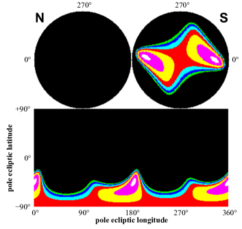
Figure 3: Example contour graph of RMS fit errors using SPA for trial pole “scans” for program object (1635) Bohrmann, showing the entire celestial sphere in ecliptic coordinates plotted in both polar and rectangular formats, with areas of best-fit poles colored white. In this case the locations of the pair of broader pole regions entirely in the south ecliptic hemisphere indicate retrograde rotation.

The remaining stages of analysis use the convex inversion (CI) method of KAAS01b, a nonlinear iterative approach. The convexinv implementation by J. Ďurech was used, guided by its accompanying documentation when choosing most of its run-time parameter settings. An exception is that for setting the the zero time $t_{0}$ and initial ellipsoid orientation angle $\phi_{0}$ the suggestion of KAAS01b was followed instead, choosing values that align the long axis of the model shape along the $x$-axis. Doing so avoids very large adjustments to the model during the first several fit iterations which can distort the ultimate outcome. Thus $t_{0}$ was set to be the time of a brightness minimum from the filtered Fourier series for a lightcurve recorded at among the smallest available solar phase angles, and then $\phi_{0}$ was calculated as the corresponding pole-dependent asterocentric longitude of the sub-PAB point (TAYL79; SLIV14, Eqs. 3–8) based on the initial value supplied for the pole location. The distribution code also was modified to support user-specified values for the axial ratios of the triaxial ellipsoid used as the initial model shape, and the initial value for $a/b$ generally was selected based on the maximum amplitude from among the Fourier series-filtered observed lightcurves.

The lightcurve data were binned to a bin width of $1/50$ of the rotation period for the CI analyses. Data sets were analyzed as relative photometry, except for the three longest-rotation period objects (761) Brendelia, (1079) Mimosa, and (1618) Dawn whose single-night lightcurves, even from the longest observing nights, individually do not record enough of a rotation to determine the shape of the lightcurve without referencing brightnesses on different nights to a common zero point. To prepare these objects’ data sets for CI, data whose brightnesses had been calibrated to standard stars were referenced to a common zero-point by using available color index information, and solar phase function coefficients were included as fitted parameters for CI analysis of these lightcurves as standard-calibrated photometry. Lightcurves for these longer-period objects whose individual nights had been referenced to the same comparison star but not also put onto a standard system, instead were composited in time and in brightness into “preassembled” lightcurves of relative photometry.

Pole regions. For the third stage of the analyses, a contour graph of CI model fits’ $\chi^{2}$ goodness-of-fit value as a function of pole location was constructed to identify the pole regions. Using the known sidereal period, a series of CI trials were run on a grid pattern of trial pole coordinates having $2^{\circ}$-resolution in latitude and longitude to systematically cover the ecliptic hemisphere indicated by SPA, in each case holding the pole fixed at the trial location and iterating until the step change in the RMS deviation decreased to less than 0.001. It was found that the pole region location results were relatively insensitive to weighting of the lightcurves. An individual example of pole regions located by CI is presented as Fig. 4.

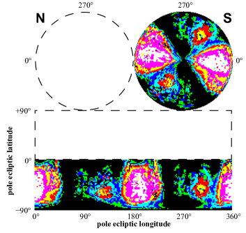
Figure 4: Similar to Fig. 3 but using CI and calculated only for trial poles in the southern ecliptic hemisphere. The pair of pole region locations favored by the lowest $\chi^{2}$ values agrees with those of the SPA regions.

Although pole regions also already are available from the epochs analysis, the program objects data sets’ are large enough to expect that the CI region locations will be more reliable, because SPA pole longitudes can be subject to systematic errors depending on the degree to which the epochs depart from the assumption that they all correspond to the same asterocentric longitude. The SPA region results did prove useful, however, to distinguish the correct solutions when CI allowed more than one possible pair of pole regions. The remaining symmetric pole ambiguity for the program objects cannot be resolved using Earth-based lightcurves, because these asteroids all share low orbital inclinations of 1 to 3 degrees as members of the Koronis family. A discussion of symmetry and ambiguities pertinent to pole solutions obtained from lightcurves can be found in MAGN89.

Spin poles. In the fourth stage CI was run to determine a best-fit period, pole, and preliminary possible model shape, using the initial period from SPA and an initial pole location estimated from the CI contour graph. For the benefit mainly of the preliminary shape model a final version of the binned lightcurve data input was constructed, weighted typically so that the number of fitted data points per apparition is proportional to its available rotation phase coverage, to within a factor of about 1.5. Any process adjustments needed for a particular object are described in its individual notes.

For these runs of CI, the criterion for stopping the fit iterations was given more deliberate consideration than was for the earlier runs to generate the pole regions contour map. As an aid in determining at what point to stop the fitting, the distribution code was modified to add to the fit iteration log at each step the fractional change in the $\chi^{2}$ goodness-of-fit metric, and the current sidereal period and pole coordinates. It was found that convergence of the period and pole were straightforward for these data sets, but how much longer to keep adjusting the model shape after the period and pole had converged was not as clear-cut and remained somewhat subjective; analyses of certain data sets showed indications that overfitting could be an issue. The guideline ultimately adopted was to iterate past period and pole convergence only until the step change in the fit relative $\chi^{2}$ decreased to less than about 0.5%.

Each preliminary model shape result was checked for consistency with an assumption of of stable rotation about its shortest axis, by constructing the corresponding model shape rendering and confirming that its shortest dimension lies along the polar axis. To solve for the shape model convex polyhedron from its facet areas and normals, a C translation of the FORTRAN code for Minkowski minimization from the CI distribution was used.

The expected symmetry of an object’s two ambiguous pole solutions with respect to the “photometric great circle” (PGC) (MAGN89) was used to perform a self-consistency check on each pair of derived pole solutions, as a significant departure from symmetry would indicate the presence of some problem with the analysis. Appendix LABEL:APDX-PGC details how symmetric poles were calculated using objects’ orbit elements.

Errors were estimated after a solution had passed both consistency checks. The period error was estimated from SPA with the full set of Fourier-filtered epochs for a pole at the adopted location. Uncertainties for the pole locations were estimated from the CI model fits’ $\chi^{2}$ distributions in each case by identifying a constant-$\chi^{2}$ contour that encloses a region just large enough to entirely surround the insignificant fluctuations near the pole location within an approximately oval-shaped region. The contour’s angular extents in ecliptic latitude and longitude were adopted as coarse estimates of $\sim 2\sigma$ confidence, and each error was rounded to the nearest multiple of $5^{\circ}$ of arc. The factor of $\sim 2$ relationship between the subjective identification of contours and the estimated error is based on comparison of the published CI pole error estimates of previously-studied objects (SLIV03; SLIV09) with their CI model fits’ $\chi^{2}$ distributions.

Model shape and axial ratios. In the last stage of the analysis, the final shape renderings and axial ratios corresponding to the best-fit period and pole results were obtained using the conjgradinv implementation from the CI distribution, which uses the facet areas directly rather than using spherical harmonics. The axial ratios for its initial ellipsoid were estimated from the preliminary model shape.

3.1 Spin and shape results

The lightcurves reported in Sec. 2 were combined with lightcurves of the program objects previously published by SLIV08a (46 apparitions) and by BINZ87 (6 apparitions), plus lightcurves from 10 more apparitions whose sources are given in the analysis descriptions for their specific objects. Table 7 summarizes for each asteroid’s available combined lightcurve data set the span of years included, the number of apparitions $N_{\rm ap}$, and aspect information as a list of ecliptic longitudes $\lambda_{\rm PAB}$ of the asteroids’ phase angle bisector (PAB) near the mid-date of the observations from each apparition.

Table 7: Summary of lightcurve observations used for spin vector analyses.

Asteroid	Years observed	$N_{\rm ap}$	$\lambda_{\rm PAB}$ of aspects observed $(^{\circ})$
(658) Asteria	1983–2007	6	53, 68, 167, 323, 340, 352
(761) Brendelia	2001–2013	7	75, 90, 158, 170, 183, 260, 353
(811) Nauheima	1984–2007	7	9, 98, 174, 239, 253, 340, 347
(975) Perseverantia	1990–2013	8	74, 97, 176, 197, 218, 267, 296, 357
(1029) La Plata	1975–2007	7	32, 78, 141, 173, 228, 328, 350
(1079) Mimosa	1983–2021	8	20, 43, 68, 120, 235, 247, 319, 329
(1100) Arnica	1999–2014	9	20, 32, 99, 104, 111, 115, 183, 188, 279
(1245) Calvinia	1977–2012	7	8, 15, 26, 107, 186, 269, 323
(1336) Zeelandia	1999–2014	9	72, 91, 125, 140, 155, 170, 245, 335, 352
(1350) Rosselia	1975–2007	8	72, 89, 149, 162, 162, 240, 284, 335
(1423) Jose	2002–2007	5	41, 139, 206, 218, 290
(1482) Sebastiana	1984–2007	7	19, 66, 151, 230, 244, 319, 333
(1618) Dawn	2003–2021	6	25, 75, 99, 187, 205, 299
(1635) Bohrmann	2003–2012	7	1, 20, 95, 110, 192, 273, 290
(1725) CrAO	2003–2019	7	95, 171, 236, 253, 341, 353, 356
(1742) Schaifers	1983–2016	7	32, 51, 129, 142, 217, 289, 350
(1848) Delvaux	2004–2015	7	79, 140, 152, 164, 259, 336, 349
(2144) Marietta	1999–2016	7	28, 108, 120, 145, 220, 230, 313
(2209) Tianjin	1996–2016	6	57, 89, 162, 178, 278, 351

The spin vector results for the program objects are presented in Table 8. The first three columns list the asteroid, its derived sidereal period $P_{\rm sid}$, and its period error. The symmetric pair of pole solutions is given in the next two groups of three columns, each grouped as a pole identifier followed by its J2000 ecliptic coordinates $(\lambda_{0};\beta_{0})$. For convenient reference the pole ID notation previously used by SLIV03; SLIV09 is retained, in which $P_{{}_{1}}$ and $P_{{}_{2}}$ denote prograde poles and $P_{{}_{3}}$ and $P_{{}_{4}}$ denote retrograde poles. The last two columns in the table give the estimated uncertainties for both poles’ longitudes and latitudes respectively in degrees of arc.

Table 8: Spin vector results.

Asteroid	$P_{\rm sid}$	$\sigma(P_{\rm sid})$	Pole	$\lambda_{0}$	$\beta_{0}$	Pole	$\lambda_{0}$	$\beta_{0}$	$\sigma(\lambda_{0})$	$\sigma(\beta_{0})$
	(h)	(h)	ID	$(^{\circ})$	$(^{\circ})$	ID	$(^{\circ})$	$(^{\circ})$	$(^{\circ})$	$(^{\circ})$
(658) Asteria	$21.02981$	$0.00003$	$P_{{}_{3}}$	124	$-$36	$P_{{}_{4}}$	306	$-$39	5	5
(761) Brendelia	$57.9949$	$0.0003$	$P_{{}_{3}}$	37	$-$47	$P_{{}_{4}}$	212	$-$48	5	10
(811) Nauheima	$4.000948$	$0.000002$	$P_{{}_{1}}$	150	$+$63	$P_{{}_{2}}$	343	$+$60	5	5
(975) Perseverantia	$7.223875$	$0.000005$	$P_{{}_{3}}$	67	$-$55	$P_{{}_{4}}$	238	$-$58	5	10
(1029) La Plata	$15.310657$	$0.000003$	$P_{{}_{1}}$	98	$+$60	$P_{{}_{2}}$	281	$+$55	5	10
(1079) Mimosa	$64.72834$	$0.00012$	$P_{{}_{3}}$	137	$-$37	$P_{{}_{4}}$	318	$-$39	5	10
(1100) Arnica	$14.53191$	$0.00002$	$P_{{}_{1}}$	123	$+$28	$P_{{}_{2}}$	301	$+$28	5	10
(1245) Calvinia	$4.8514754$	$0.0000005$	$P_{{}_{3}}$	54	$-$50	$P_{{}_{4}}$	235	$-$43	5	5
(1336) Zeelandia	$15.60188$	$0.00003$	$P_{{}_{1}}$	45	$+$5	$P_{{}_{2}}$	226	$+$11	5	5
(1350) Rosselia	$8.140103$	$0.000002$	$P_{{}_{3}}$	131	$-$84	$P_{{}_{4}}$	269	$-$80	5	5
(1423) Jose	$12.312679$	$0.000010$	$P_{{}_{3}}$	98	$-$80	$P_{{}_{4}}$	237	$-$82	5	5
(1482) Sebastiana	$10.489660$	$0.000003$	$P_{{}_{3}}$	93	$-$78	$P_{{}_{4}}$	237	$-$79	5	5
(1618) Dawn	$43.22002$	$0.00012$	$P_{{}_{3}}$	101	$-$57	$P_{{}_{4}}$	268	$-$58	5	5
(1635) Bohrmann	$5.864286$	$0.000003$	$P_{{}_{3}}$	9	$-$46	$P_{{}_{4}}$	194	$-$46	5	10
(1725) CrAO	$21.47246$	$0.00007$	$P_{{}_{3}}$	64	$-$39	$P_{{}_{4}}$	241	$-$33	5	5
(1742) Schaifers	$8.532708$	$0.000002$	$P_{{}_{1}}$	27	$+$71	$P_{{}_{2}}$	195	$+$75	5	5
(1848) Delvaux	$3.63911184$	$0.00000019$	$P_{{}_{3}}$	143	$-$83	$P_{{}_{4}}$	348	$-$82	5	5
(2144) Marietta	$5.4885454$	$0.0000012$	$P_{{}_{1}}$	145	$+$72	$P_{{}_{2}}$	344	$+$70	5	5
(2209) Tianjin	$9.452694$	$0.000003$	$P_{{}_{1}}$	19	$+$68	$P_{{}_{2}}$	186	$+$72	5	5

The spin obliquity $\varepsilon$ of each pole solution, calculated as the angle between the spin pole and the orbit pole, is given in Table 9. In the context of the spin poles, “prograde” and “retrograde” refer to poles whose obliquities are less than $90^{\circ}$ and greater than $90^{\circ}$, respectively. “High obliquities” are near $90^{\circ}$ and near the orbit plane; “low obliquities” are near either $0^{\circ}$ (prograde) or $180^{\circ}$ (retrograde) and near perpendicular to the orbit plane. Owing to the small orbital inclinations of the Koronis family, the obliquities of the two poles comprising each symmetric pair differ by less than $2^{\circ}$, well within the estimated uncertainties of the pole locations. In the last column the mean of each pair of obliquities is given as a single adopted mean obliquity for the object.

Table 9: Spin obliquities for the spin vectors given in Table 8.

Asteroid	Orbit pole${}^{\rm a}$	Spin vector obliquities				Adopted $\varepsilon$
(658) Asteria	(261${}^{\circ}$;$+$88${}^{\circ}$)	$P_{{}_{3}}$	127${}^{\circ}$	$P_{{}_{4}}$	128${}^{\circ}$	127${}^{\circ}$
(761) Brendelia	(294${}^{\circ}$;$+$88${}^{\circ}$)	$P_{{}_{3}}$	138${}^{\circ}$	$P_{{}_{4}}$	138${}^{\circ}$	138${}^{\circ}$
(811) Nauheima	(41${}^{\circ}$;$+$87${}^{\circ}$)	$P_{{}_{1}}$	28${}^{\circ}$	$P_{{}_{2}}$	28${}^{\circ}$	28${}^{\circ}$
(975) Perseverantia	(309${}^{\circ}$;$+$87${}^{\circ}$)	$P_{{}_{3}}$	146${}^{\circ}$	$P_{{}_{4}}$	147${}^{\circ}$	147${}^{\circ}$
(1029) La Plata	(300${}^{\circ}$;$+$88${}^{\circ}$)	$P_{{}_{1}}$	32${}^{\circ}$	$P_{{}_{2}}$	33${}^{\circ}$	32${}^{\circ}$
(1079) Mimosa	(240${}^{\circ}$;$+$89${}^{\circ}$)	$P_{{}_{3}}$	127${}^{\circ}$	$P_{{}_{4}}$	129${}^{\circ}$	128${}^{\circ}$
(1100) Arnica	(214${}^{\circ}$;$+$89${}^{\circ}$)	$P_{{}_{1}}$	62${}^{\circ}$	$P_{{}_{2}}$	62${}^{\circ}$	62${}^{\circ}$
(1245) Calvinia	(62${}^{\circ}$;$+$87${}^{\circ}$)	$P_{{}_{3}}$	137${}^{\circ}$	$P_{{}_{4}}$	136${}^{\circ}$	136${}^{\circ}$
(1336) Zeelandia	(7${}^{\circ}$;$+$87${}^{\circ}$)	$P_{{}_{1}}$	83${}^{\circ}$	$P_{{}_{2}}$	82${}^{\circ}$	82${}^{\circ}$
(1350) Rosselia	(50${}^{\circ}$;$+$87${}^{\circ}$)	$P_{{}_{3}}$	172${}^{\circ}$	$P_{{}_{4}}$	172${}^{\circ}$	172${}^{\circ}$
(1423) Jose	(329${}^{\circ}$;$+$87${}^{\circ}$)	$P_{{}_{3}}$	171${}^{\circ}$	$P_{{}_{4}}$	172${}^{\circ}$	171${}^{\circ}$
(1482) Sebastiana	(341${}^{\circ}$;$+$87${}^{\circ}$)	$P_{{}_{3}}$	169${}^{\circ}$	$P_{{}_{4}}$	169${}^{\circ}$	169${}^{\circ}$
(1618) Dawn	(13${}^{\circ}$;$+$87${}^{\circ}$)	$P_{{}_{3}}$	147${}^{\circ}$	$P_{{}_{4}}$	148${}^{\circ}$	148${}^{\circ}$
(1635) Bohrmann	(95${}^{\circ}$;$+$88${}^{\circ}$)	$P_{{}_{3}}$	136${}^{\circ}$	$P_{{}_{4}}$	136${}^{\circ}$	136${}^{\circ}$
(1725) CrAO	(29${}^{\circ}$;$+$87${}^{\circ}$)	$P_{{}_{3}}$	127${}^{\circ}$	$P_{{}_{4}}$	126${}^{\circ}$	126${}^{\circ}$
(1742) Schaifers	(62${}^{\circ}$;$+$88${}^{\circ}$)	$P_{{}_{1}}$	17${}^{\circ}$	$P_{{}_{2}}$	17${}^{\circ}$	17${}^{\circ}$
(1848) Delvaux	(242${}^{\circ}$;$+$89${}^{\circ}$)	$P_{{}_{3}}$	173${}^{\circ}$	$P_{{}_{4}}$	173${}^{\circ}$	173${}^{\circ}$
(2144) Marietta	(49${}^{\circ}$;$+$87${}^{\circ}$)	$P_{{}_{1}}$	19${}^{\circ}$	$P_{{}_{2}}$	19${}^{\circ}$	19${}^{\circ}$
(2209) Tianjin	(61${}^{\circ}$;$+$87${}^{\circ}$)	$P_{{}_{1}}$	20${}^{\circ}$	$P_{{}_{2}}$	19${}^{\circ}$	19${}^{\circ}$

${}^{\rm a}$ The orbit pole is ($\Omega-$90${}^{\circ}$; 90${}^{\circ}-i$) where the values of the osculating orbit elements used, longitude of ascending node $\Omega$ and inclination $i$, are ecliptic and equinox J2000.0 for epoch JD 2451800.5 (EMP2000).