Study of charm and beauty in QGP from unquenched lattice QCD

Abstract

We present charmonium and bottomonium correlators and corresponding reconstructed spectral functions from full QCD calculations in the pseudoscalar channel. Correlators are obtained using a mixed-action approach, clover-improved Wilson valence quarks on gauge field configurations generated with $N_{f}=2+1$ HISQ sea quarks, with physical strange quark masses and light quark masses corresponding to $m_{\pi}=315$ MeV. The charm and bottom quark masses are tuned to reproduce the experimental mass spectrum of the spin averaged quarkonium vector mesons from the particle data group [1]. For the spectral reconstruction, we use models based on perturbative spectral functions from different frequency regions like resummed thermal contributions around the threshold from pNRQCD [2] and vacuum contributions well above the threshold [3]. We show preliminary results of the reconstructed spectral function obtained for the first time in our study for full QCD.

1 Introduction

The spectrum of bound states of heavy quark and anti-quark pairs, the so-called quarkonia may receive thermal modifications in the hot QCD medium. To investigate such thermal effects the correlator in the pseudoscalar channel is an ideal choice because, unlike the vector channel, the spectral function embedded in it has no transport peak in the low-frequency region i.e. $|\omega|<<T^{2}/M$ [4, 5, 6, 7], where $M$ is a heavy quark mass, and $T$ is the temperature. The Consideration of the pseudoscalar channel excludes the modeling of the transport peak. The Euclidean time pseudoscalar correlator reads

$$G_{\mbox{\scriptsize PS}}(\tau) \equiv M_{B}^{2}\int_{\vec{x}}\Bigl{\langle}(\bar{\psi}\gamma_{5}\psi)(\tau,\vec{x})(\bar{\psi}\gamma_{5}\psi)(0,\vec{0})\Bigr{\rangle}_{c},$$ (1)

where $M_{B}$ is the bare quark mass and $\psi$ is the Dirac spinor. $\langle...\rangle_{c}$ represents that only the connected diagrams are considered in this study. The correlator $G_{PS}(\tau)$ is computed numerically on the 4d hypercubic lattice and it is related to the corresponding spectral function $\rho_{\mbox{\scriptsize PS}}(\omega)$ through the equation

$$G_{\mbox{\scriptsize PS}}(\tau)\;=\;\int_{0}^{\infty}\frac{{\rm d}\omega}{\pi}\rho_{\mbox{\scriptsize PS}}(\omega)\frac{\cosh\left(\left(\frac{1}{2T}-\tau\right)\omega\right)}{\sinh\left(\frac{\omega}{2T}\right)}\;.$$ (2)

For given $G_{\mbox{\scriptsize PS}}(\tau)$, Eq. (2) can be solved for $\rho_{\mbox{\scriptsize PS}}(\omega)$ but the solution is not unique [8, 9]. The nature of the function $\frac{\cosh\left(\left(\frac{1}{2T}-\tau\right)\omega\right)}{\sinh\left(\frac{\omega}{2T}\right)}$ is such that a small change in $G_{\mbox{\scriptsize PS}}(\tau)$ may lead to large uncertainty in the spectral function. There might be several spectral functions that all fit into the correlator data, but which one is correct is hard to determine. Therefore we need some theoretically or phenomenologically motivated input to constrain the search space. One of the possibilities is to construct the spectral function by taking input from perturbation theory or effective field theories like pNRQCD. In this study we follow the strategy developed in the quenched approximation [10].

2 Lattice Setup

We compute quarkonium correlators using clover-improved Wilson fermions as valence quarks at different temperatures listed in Tab. 1. The measurements are done on $N_{f}$=2+1, $m_{l}=m_{s}/5$ HISQ gaugefield configurations generated by the HotQCD collaboration. The clover improvement in the fermion valence action reduces $O(a)$ cut-off effects. This improvement is made by choosing the Sheikholeslami-Wohlert coefficient $c_{SW}=\frac{1}{u^{3}_{0}}$ [11], where $u_{0}$ is the tadpole factor and is calculated as the fourth root of the plaquette expectation value calculated on HISQ lattices.

$\beta$	$a$[fm]	$a^{-1}$[GeV]	$N_{\sigma}$	$N_{\tau}$	$T$[MeV]	$\#$ confs
8.249	0.028	7.033	64	64	110	112
			96	56	126	200
			96	32	220	1703
			96	28	251	621

Table 1: Lattice parameters for $N_{f}$=2+1, $m_{l}=m_{s}/5$ HISQ configurations. At $\beta$=8.249 the lattice spacing $a$ is obtained using $f_{k}$-scale parametrization [12].

3 Clover mass tuning on mixed action

The masses of hadrons from lattice QCD also depend on another parameter, the bare quark mass, $m_{q}$, which for Wilson fermions is tuned by the so-called hopping parameter $\kappa$ defined as $\kappa=\frac{1}{8+2m_{q}}$. To obtain numerical data of mesonic correlators at physical quark mass, one needs to tune the quark mass such that the meson mass from the lattice is consistent with the corresponding experimental value. In the heavy quark sector, we tune to the spin averaged charmonium $m_{c\bar{c}}=(m_{\eta_{c}}+3m_{J/\psi})/4$ and bottomonium $m_{b\bar{b}}=(m_{\eta_{b}}+3m_{\Upsilon})/4$. Fig. 1 illustrates the charm quark mass tuning, where $am^{phy}_{c\bar{c}}$ is the physical mass in lattice units. The tuned $\kappa$ values for charm and bottom are 0.13164 and 0.11684, respectively.

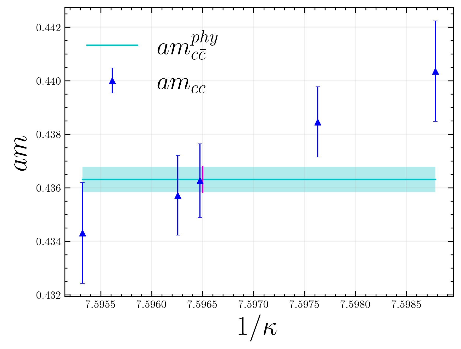
Figure 1: Charm quark mass tuning on the mixed action. The solid line represents the experimental value of the spin-averaged charmonium in lattice units taken from the PDG. Whereas triangles represent masses from lattice calculations for different values of $\kappa$ in lattice units.

4 Correlators

To obtain quarkonium spectral functions in the pseudoscalar channel one needs the numerical correlator data computed on the lattice. Fig. 2 shows the data measured by clover-improved Wilson fermions on large $N_{f}$=2+1 HISQ gaugefield configurations. Instead of the correlator itself, we used the ratio $G_{\mbox{\scriptsize PS}}(\tau)/G^{\mbox{\scriptsize free}}_{\mbox{\scriptsize PS}}(\tau)$ so that one can see the behavior as a function of $\tau$ at various temperatures, where $G^{\mbox{\scriptsize free}}_{\mbox{\scriptsize PS}}(\tau)$ reads [10]

$$\frac{G_{\mbox{\scriptsize PS}}^{\mbox{\scriptsize free}}(\tau)}{m^{2}(\bar{\mu}_{\mbox{\scriptsize ref}})} \equiv \int_{2M_{\mbox{\scriptsize 1S}}}^{\infty}\!\frac{{\rm d}\omega}{\pi}\,\biggl{\{}\frac{N_{\rm c}\omega^{2}}{8\pi}\tanh\Bigl{(}\frac{\omega}{4T}\Bigr{)}\sqrt{1-\frac{4M_{\mbox{\scriptsize 1S}}^{2}}{\omega^{2}}}\biggr{\}}\,\frac{\cosh\left(\left(\frac{1}{2T}-\tau\right)\omega\right)}{\sinh\left(\frac{\omega}{2T}\right)}\;,$$ (3)

where $m(\bar{\mu}_{\mbox{\scriptsize ref}})$ is the running mass at reference scale $\bar{\mu}_{\mbox{\scriptsize ref}}$=2 GeV. We choose the values of $M_{\mbox{\scriptsize 1S}}$ to be 1.5 GeV for charmonium and 4.7 GeV for bottomonium. One can see that the charmonium suffers more thermal effects than the bottomonium as the charmonium correlators at high temperatures deviate more from the low-temperature ones.

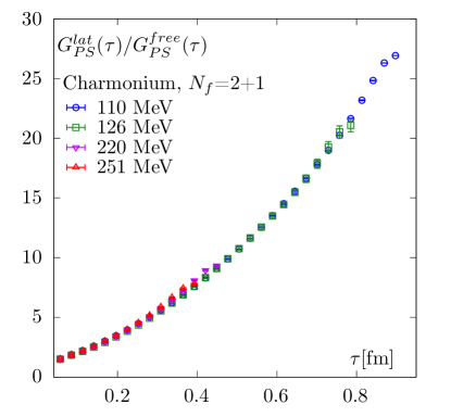
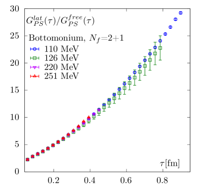
Figure 2: Average values of correlator ratios at different temperatures for pseudoscalar quarkonium correlators.

5 Perturbative spectral functions in PS-channel

To construct the quarkonium spectral functions in the pseudoscalar channel we follow the strategy developed in the quenched approximation [10]. We first consider thermal contributions around the threshold i.e. $\omega\approx 2M$. Well above the threshold the thermal effects are power suppressed, and the spectral function can be replaced by the vacuum one. In the heavy quark mass limit, relativistic effects can be ignored. In this case, one can get the pseudoscalar spectral function from the vector channel as

$$\rho^{\mbox{\scriptsize pNRQCD}}_{\mbox{\scriptsize PS}}=\frac{M^{2}}{3}\rho^{\mbox{\scriptsize pNRQCD}}_{\mbox{\scriptsize V}}\;,\quad\omega\approx 2M\;.$$ (4)

One can get the vector spectral function by applying pNRQCD calculations as

$$\rho^{\mbox{\scriptsize pNRQCD}}_{\mbox{\scriptsize V}}(\omega)=\frac{1}{2}\Bigl{(}1-e^{-\frac{\omega}{T}}\Bigr{)}\int_{-\infty}^{\infty}\!{\rm d}t\,e^{i\omega t}\;C_{>}(t;{\vec{0},\vec{0}})\;,$$ (5)

where $C_{>}$ is a Wightman function and it is obtained by solving the following differential equation

$$\biggl{\{}i\partial_{t}-\biggl{[}2M+V_{\mbox{\scriptsize$T$}}(r)-\frac{\nabla^{2}_{\vec{r}}}{M}\biggr{]}\biggr{\}}\,C_{>}^{V}(t;{\vec{r},\vec{r^{\prime}}})=0\;,\quad t\neq 0\;,$$ (6)

with initial conditions $C_{>}^{V}(0;{\vec{r},\vec{r^{\prime}}})=6N_{\rm c}\,\delta^{(3)}({\vec{r}-\vec{r^{\prime}}})\;$. The potential $V_{\mbox{\scriptsize$T$}}(r)$ for positive $t$ has the following form [13, 14, 15]

$$V_{\mbox{\scriptsize$T$}}(r)=-\alpha_{\mbox{\scriptsize s}}C_{F}\biggl{[}m_{\mbox{\scriptsize D}}+\frac{\exp(-m_{\mbox{\scriptsize D}}r)}{r}\biggr{]}-{i\alpha_{\mbox{\scriptsize s}}C_{\mbox{\scriptsize F}}T}\,\phi(m_{\mbox{\scriptsize D}}r)+{\mathcal{O}}(\alpha_{\mbox{\scriptsize s}}^{2})\;.$$ (7)

Here $\phi(x)$ is defined to be

$$\phi(x)\equiv 2\int_{0}^{\infty}\!\frac{{\rm d}z\,z}{(z^{2}+1)^{2}}\biggl{[}1-\frac{\sin(zx)}{zx}\biggr{]}.$$ (8)

At $\omega<2M$, the spectral function is overestimated. To correct this, we multiply $e^{-|\omega-2M|/T}$ to $\phi$. Moreover, at small spatial distances, $r\ll 1/m_{\mbox{\scriptsize D}}$, the thermal potential is replaced by a vacuum one [10].

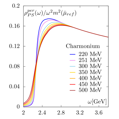
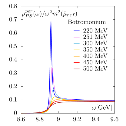
Figure 3: Perturbative spectral functions, in the pseudoscalar channel normalised by $\omega^{2}m^{2}(\bar{\mu}_{ref})$ as a function of $\omega$ for charmonium and bottomonium at various temperatures.

For $\omega>2M$, the spectral function is insensitive to temperature effects, therefore we also replace it by its vacuum counterpart, which we calculate following [10] and references therein. The vacuum spectral function, normalised by $\omega^{2}m^{2}(\bar{\mu})$, in the pseudoscalar channel reads

$$\left.\frac{\rho_{\mbox{\scriptsize PS}}(\omega)}{\omega^{2}m^{2}(\bar{\mu})}\right|^{\mbox{\scriptsize vac}}\;\equiv\;\frac{N_{\rm c}}{8\pi}\,\tilde{R}_{\mbox{\scriptsize c}}^{p}(\omega)\;.$$ (9)

$R$-function is defined as

$$\tilde{R}_{\mbox{\scriptsize c}}^{p}(\omega) = \tilde{R}^{p(0)}(\omega)+\frac{\alpha_{\mbox{\scriptsize s}}(\bar{\mu})}{\pi}\,C_{\mbox{\scriptsize F}}\tilde{R}^{p(1)}(\omega)$$ (10)

$$+ \biggl{(}\frac{\alpha_{\mbox{\scriptsize s}}(\bar{\mu})}{\pi}\biggr{)}^{2}\Bigl{[}C_{\mbox{\scriptsize F}}^{2}\,\tilde{R}^{p(2)}_{A}(\omega)+C_{\mbox{\scriptsize F}}N_{\rm c}\,\tilde{R}^{p(2)}_{N\!A}(\omega)+C_{\mbox{\scriptsize F}}T_{\mbox{\scriptsize F}}N_{\rm f}\,\tilde{R}^{p(2)}_{l}(\omega)\Bigr{]}+{\mathcal{O}}(\alpha_{\mbox{\scriptsize s}}^{3})\;,\hskip 17.07164pt$$

where $T_{\mbox{\scriptsize F}}\equiv 1/2$, $C_{\mbox{\scriptsize F}}\equiv(N_{\rm c}^{2}-1)/(2N_{\rm c})$ and

$$\tilde{R}^{p(0)} \stackrel{{\scriptstyle\omega\gg m(\bar{\mu})}}{{\approx}} 1\;,$$ (11)

$$\tilde{R}^{p(1)} \stackrel{{\scriptstyle\omega\gg m(\bar{\mu})}}{{\approx}} \frac{3}{2}\ln\biggl{(}\frac{\bar{\mu}^{2}}{\omega^{2}}\biggr{)}+\frac{17}{4}\;,$$ (12)

$$\tilde{R}^{p(2)}_{A} \stackrel{{\scriptstyle\omega\gg m(\bar{\mu})}}{{\approx}} \frac{9}{8}\ln^{2}\biggl{(}\frac{\bar{\mu}^{2}}{\omega^{2}}\biggr{)}+\frac{105}{16}\ln\biggl{(}\frac{\bar{\mu}^{2}}{\omega^{2}}\biggr{)}+\frac{691}{64}-\frac{9\zeta_{2}}{4}-\frac{9\zeta_{3}}{4}\;,$$ (13)

$$\tilde{R}^{p(2)}_{N\!A} \stackrel{{\scriptstyle\omega\gg m(\bar{\mu})}}{{\approx}} \frac{11}{16}\ln^{2}\biggl{(}\frac{\bar{\mu}^{2}}{\omega^{2}}\biggr{)}+\frac{71}{12}\ln\biggl{(}\frac{\bar{\mu}^{2}}{\omega^{2}}\biggr{)}+\frac{893}{64}-\frac{11\zeta_{2}}{8}-\frac{31\zeta_{3}}{8}\;,$$ (14)

$$\tilde{R}^{p(2)}_{l} \stackrel{{\scriptstyle\omega\gg m(\bar{\mu})}}{{\approx}} -\frac{1}{4}\ln^{2}\biggl{(}\frac{\bar{\mu}^{2}}{\omega^{2}}\biggr{)}-\frac{11}{6}\ln\biggl{(}\frac{\bar{\mu}^{2}}{\omega^{2}}\biggr{)}-\frac{65}{16}+\frac{\zeta_{2}}{2}+\zeta_{3}\;.$$ (15)

After computing both thermal and vacuum contributions to the spectral function, we combine them as

$$\begin{split}\rho_{\mbox{\scriptsize PS}}^{\mbox{\scriptsize pert}}(\omega)=A^{\mbox{\scriptsize match}}\rho^{{\mbox{\scriptsize pNRQCD}}}_{\mbox{\scriptsize PS}}(\omega)\theta(\omega^{\mbox{\scriptsize match}}-\omega)+\rho^{\mbox{\scriptsize vac}}_{\mbox{\scriptsize PS}}(\omega)\theta(\omega-\omega^{\mbox{\scriptsize match}})\;.\end{split}$$ (16)

In Eq. (16) we introduce a multiplicative factor $A^{\mbox{\scriptsize match}}$ to the thermal part and it is determined such that both thermal and vacuum parts of the spectral function are connected smoothly at some $\omega=\omega^{\mbox{\scriptsize match}}$, where $2M<\omega^{\mbox{\scriptsize match}}<3M$. The resulting pseudoscalar spectral functions at various temperatures for both charmonium and bottomonium are shown in Fig. (3). Unlike charmonium, the bottomoniun has a resonance peak that is visible at temperatures below 300 MeV, and above 300 MeV bottomonium starts melting.

6 Spectral reconstruction

In this section we will discuss how to model the perturbative spectral functions and obtain reconstructed spectral functions. To accommodate the normalization of the correlator data and a possible thermal mass shift, we introduce two additional parameters $A$ and $B$ to the perturbative spectral function showed in Fig. (3). The model spectral function reads

$$\rho^{\mbox{\scriptsize mod}}_{\mbox{\scriptsize PS}}(\omega)=A\rho^{\mbox{\scriptsize pert}}_{\mbox{\scriptsize PS}}(\omega-B)\;.$$ (17)

This model spectral function is fitted to the unrenormalized pseudoscalar lattice correlator that is shown in Fig. (2), at $T$=251 MeV to determine the parameters $A$ and $B$. Fitting the renormalized correlator may change the value of $A$, but $B$ will remain unchanged. Preliminary results for the model spectral function $\rho^{\mbox{\scriptsize mod}}$ and original correlator data are shown in Fig. (4).

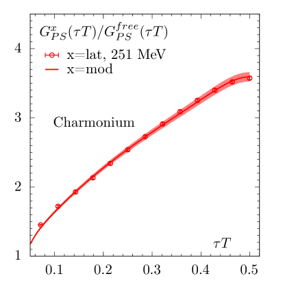
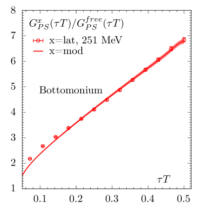
Figure 4: Data points represent the original lattice correlator whereas lines represent model correlator obtained from Eq. (2) for charmonium (left) and bottomonium. (right).

7 Conclusion and Outlook

We have presented preliminary results of pseudoscalar charmonium and bottomonium correlation functions obtained from clover-improved Wilson valence quarks on $2+1$-flavor HISQ gauge field configurations with physical strange quark masses and light quark masses with $m_{l}=m_{s}/5$ corresponding to $m_{\pi}$=315 MeV at a temperature of $T$=251 MeV. The tuning of the quark masses was done at zero temperature by comparing the spin-averaged quarkonium mass with their corresponding experimental values taken from the particle data group. We have constructed the perturbative spectral function in the pseudoscalar channel by smoothly matching the thermal and vacuum parts. A model is formulated by introducing two parameters to the perturbative spectral function. The values of the parameters are determined by fitting the model to the lattice correlator data. The model describes the lattice data reasonably well at large time-slice separations. However, at a small distance, there is a discrepancy which might be due to cut-off effects because our measurements are still at finite lattice spacing. To study the cut-off effects we will add additional lattice spacings and finally perform a continuum extrapolation of the correlation functions, which is work in progress. This will extend the previous study in the quenched approximation [10] towards full QCD. We also plan to add more temperatures to study the in-medium modifications of quarkonium states in the relevant temperature region for heavy ion collision experiments. The dynamical light quark degrees of freedom are still unphysical in this study. Although the dependence of light degrees of freedom on the heavy quark sector may be small, to check this dependence we plan to add calculations at physical light quark masses. This study will also be extended to the vector channel, i.e. unquenching the results [16] on the in-medium modification of charmonium and bottomonium vector mesons and charm and bottom diffusion coefficients.

8 ACKNOWLEDGMENTS

We thank Mikko Laine for helpful and elucidating discussions. We also thank Luis Altenkort for the production of gauge configurations and the implementation of meson measurements in the QUDA code. This work is supported by the Deutsche Forschungsgemeinschaft (DFG, German Research Foundation)-Project number 315477589-TRR 211. The computations in this work were performed on the GPU cluster at Bielefeld University using SIMULATeQCD suite [17, 18] and QUDA [19]. We thank the Bielefeld HPC.NRW team for their support.

References

- [1] R. L. Workman et al. [Particle Data Group], Review of Particle Physics, PTEP 2022 (2022), 083C01.
- [2] M. Laine, A Resummed perturbative estimate for the quarkonium spectral function in hot QCD, JHEP 05, 028 (2007).
- [3] Y. Burnier and M. Laine, Towards flavour diffusion coefficient and electrical conductivity without ultraviolet contamination, Eur. Phys. J. C 72 (2012), 1902.
- [4] P. Petreczky and D. Teaney, Heavy quark diffusion from the lattice, Phys. Rev. D 73 (2006) 014508.
- [5] T. Umeda, Constant contribution in meson correlators at finite temperature, Phys. Rev. D 75 (2007) 094502.
- [6] F. Karsch, E. Laermann, P. Petreczky and S. Stickan, Infinite temperature limit of meson spectral functions calculated on the lattice, Phys. Rev. D 68 (2003), 014504.
- [7] G. Aarts and J. M. Martinez Resco, Continuum and lattice meson spectral functions at nonzero momentum and high temperature, Nucl. Phys. B 726 (2005), 93-108.
- [8] O. Kaczmarek and H. T. Shu, Spectral and Transport Properties from Lattice QCD, Lect. Notes Phys. 999 (2022), 307-345.
- [9] A. Rothkopf, Heavy Quarkonium in Extreme Conditions, Phys. Rept. 858 (2020), 1-117.
- [10] Y. Burnier, H. T. Ding, O. Kaczmarek, A. L. Kruse, M. Laine, H. Ohno, and H. Sandmeyer, Thermal quarkonium physics in the pseudoscalar channel, JHEP 11, 206 (2017).
- [11] B. Sheikholeslami and R. Wohlert, Improved Continuum Limit Lattice Action for QCD with Wilson Fermions, Nucl. Phys. B 259 (1985), 572.
- [12] A. Bazavov et al, Equation of state in (2+1)-flavor QCD, Phys. Rev. D 90 (2014) 094503.
- [13] M. Laine et al, Real-time static potential in hot QCD, JHEP 03 (2007) 054.
- [14] A. Beraudo et al, Real and imaginary-time correlators in a thermal medium, Nucl. Phys. A 806 (2008) 312.
- [15] N. Brambilla et al, Static quark-antiquark pairs at finite temperature, Phys. Rev. D 78 (2008) 014017.
- [16] H. T. Ding, O. Kaczmarek, A. L. Lorenz, H. Ohno, H. Sandmeyer and H. T. Shu, Charm and beauty in the deconfined plasma from quenched lattice QCD, Phys. Rev. D 104 (2021) 114508.
- [17] D. Bollweg, L. Altenkort, D. A. Clarke, O. Kaczmarek, L. Mazur, C. Schmidt, P. Scior and H. T. Shu, HotQCD on multi-GPU Systems, PoS LATTICE2021 (2022) 196.
- [18] L. Mazur, Topological Aspects in Lattice QCD, Ph.D. thesis, Bielefeld University, doi:10.4119/unibi/2956493.
- [19] M. A. Clark, R. Babich, K. Barros, R. C. Brower and C. Rebbi, Solving Lattice QCD systems of equations using mixed precision solvers on GPUs, Comput. Phys. Commun. 181 (2010) 1517.